Article

DEM-Based Vs30 Map and Terrain Surface Classification in Nationwide Scale—A Case Study in Iran

by
Sadra Karimzadeh
1,2,*,
Bakhtiar Feizizadeh
1,2 and
Masashi Matsuoka
3
1
Department of Remote Sensing and GIS, University of Tabriz, Tabriz 5166616471, Iran
2
Institute of Environment, University of Tabriz, Tabriz 5166616471, Iran
3
Department of Architecture and Building Engineering, School of Environment and Society, Tokyo Institute of Technology 4259-G3-2 Nagatsuta, Midori-ku, Yokohama 226-8502, Japan
*
Author to whom correspondence should be addressed.
ISPRS Int. J. Geo-Inf. 2019, 8(12), 537; https://doi.org/10.3390/ijgi8120537
Submission received: 22 October 2019 / Revised: 24 November 2019 / Accepted: 24 November 2019 / Published: 27 November 2019
(This article belongs to the Special Issue Geomatics and Geo-Information in Earthquake Studies)

Abstract

:
Different methods have been proposed to create seismic site condition maps. Ground-based methods are time-consuming in many places and require a lot of manual work. One method suggests topographic data as a proxy for seismic site condition of large areas. In this study, we mainly focused on the use of an ASTER 1c digital elevation model (DEM) to produce Vs30 maps throughout Iran using a GIS-based regression analysis of Vs30 measurements at 514 seismic stations. These maps were found to be comparable with those that were previously created from SRTM 30c data. The Vs30 results from ASTER 1c estimated the higher velocities better than those from SRTM 30c. In addition, a combination of ASTER 1c and SRTM 30c amplification maps can be useful for the detection of geological and geomorphological units. We also classified the terrain surface of six seismotectonic regions in Iran into 16 classes, considering three important criteria (slope, convexity and texture) to extract more information about the location and morphological characteristics of the stations. The results show that 98% of the stations are situated in six classes, 30% of which are in class 12, 27% in class 6, 17% in class 9, 16% in class 3, 4% in class 3and the rest of the stations are located in other classes.

1. Introduction

Recent developments in urban environments and settlement areas, as well as their complexity has led to increased demand for site condition maps [1,2,3]. In order to connect the effective parameters related with the ground motion, coordinates and geospatial analysis play an important role [4,5,6,7]. In fact, coordinates establish a unique opportunity for us to understand our surrounding areas better than we have been able to in the past. Generally, Geographical Information System (GIS) is a technology which offers potential for spatial analysis. Using either local or global coordinate systems, it connects effective but somehow discrete factors, such as Vs30 (average shear wave velocity between a 0 and 30 meter depth) and elevation data. GIS calculations based on Vs30 have been used frequently for geotechnical investigations and geomorphologic classifications on national scales [8,9,10,11].
A review of the research literature indicates that the effects of site amplifications (stratigraphy + topography) on seismic ground motion and consequently, their potential for earthquake damages, have been studied in previous work [12,13,14,15,16,17,18]. Vs30 is now one of the standard indicators for mapping seismic site conditions in most building codes of earthquake-prone countries. For instance, similarly to NEHRP (National Earthquake Hazards Program) classifications in the U.S., Iranian standard (Standard No. 2800) under the authority of the BHRC (Building & Housing Research Center) considers soil classifications as a basis for estimating Vs30 [19,20]. However, the quality and density of Vs30 measurements vary from one region to another. Additionally, sometimes, geological information of the ground surface is lacking, proves to be unavailable, or is unreliable. In this situation, continuous Vs30 measurements (cell-by-cell) from the satellite-based elevation data gain importance and become an ongoing topic in order to produce the site condition maps related with prompt seismic damage assessments. A glimpse of site classification maps for vast areas (e.g., on a national scale), shows that each of the models use specific formulation approaches and can be categorized into two main classes: (1) hybrid models which use geomorphologic, geologic and topographic data, and (2) single models which use only one item. A principal example for the first category is a nationwide site classification map of Japan developed by Matsuoka et al. [5], which made use of a multiple regression analysis to calculate the regression coefficients of 21 geomorphologic units. The Japanese QuiQuake system (a Quick estimation system for earthquake maps triggered by observation records) uses the method proposed by Matsuoka et al. [5] to provide amplification capability maps throughout Japan [21]. The site condition map of the continental United States by Allen and Wald [16] (updated by Allen and Wald [17]) is an example of the second category which utilized only topographic slope data from the Shuttle Radar Topography Mission (SRTM) 30 arcsec (~ 1km resolution near the equator) as a proxy for the site amplification. The Prompt Assessment of the Global Earthquake for Response (PAGER) used the method described by Wald and Allen [15] as a core idea for real-time damage assessments (http://earthquake.usgs.gov/eqcenter/pager/S). In recent studies for nationwide purposes, Forte et al. [22] provided seismic soil classification maps for Italy based on site-specific measurements, including Vs30 measurements and geological information. Stewart et al. [23] produced geologic and terrain-based site condition maps for California using geological information and 1, 3, 9 and 30 arcsec DEMs. The results produced by three arcsec datapoints were more accurately relative to the real measurements than other DEMs. Later, six proxy-based models for California (using geological information, topography, and geomorphological classification) were compared with the 503 Vs30 measurements and NEHRP site classes [24].
In this study, we used digital elevation data (ASTER 1 arcsec), gathered by a ASTER sensor (Advanced Spaceborne Thermal Emission and Reflection Radiometer), to understand how DEM resolutions from different sources can affect DEM-based Vs30 maps. Based on Vs30 measurements of 514 locations with strong motion seismometers in Iran, linear regression formulas for different slope classes were developed within six seismotectonic regions of Iran. Recognition of the small features can be improved in medium-resolution topographic gradient, but the derived Vs30 maps do not show significant improvements in comparison with those from low-resolution DEM.

2. Study Area

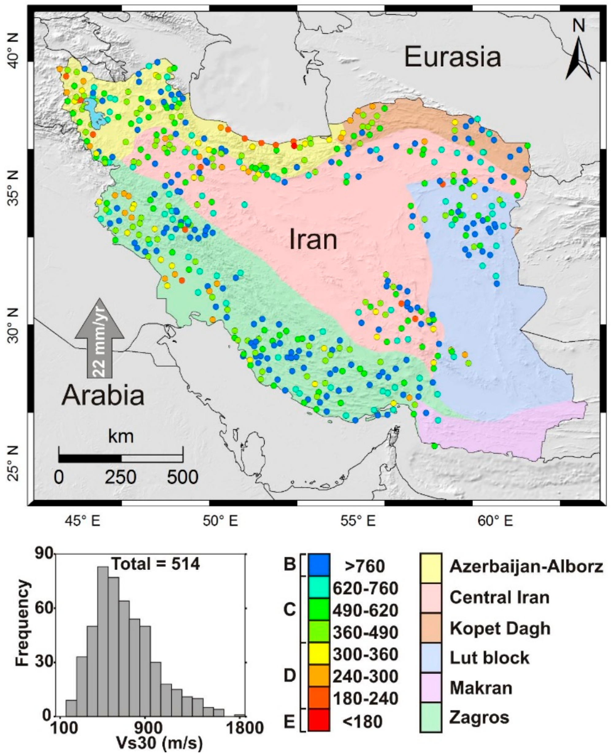
2.1. Seismotectonic Setting

Iran is trapped between the Arabian and Eurasian plates, with approximately 22 mm/yr of northward shortening [25]. The convergence of these plates shows the emergence of faults and different seismotectonic regions in Iran (Figure 1). Different seismotectonic regions have been identified for Iran, typically from the geographical and historical distributions of active faults and structural trends [26,27,28,29]. The main seismotectonic regions in Iran are as follows: (1) Alborz-Azarbaijan, (2) Central Iran, (3) Kopet Dagh, (4) Lut, (5) Makran, and (6) Zagros. Alborz-Azarbaijan and Zagros are the most populated blocks which absorb the main portion of continental shortening and consequently, the number of earthquakes in these blocks is considerably higher than elsewhere [25]. From the Bayesian estimation, the seismic hazard is lowest in the Lut and Central Iran blocks, meaning that these blocks are craton [30]. Slope classes in active tectonic regions are different from craton parts. Ideally, in the regression analyses, active and stable areas should be separated during Vs30 calculations, but due to large investments on geotechnical and seismological investigations in highly populated regions, a significant portion of our Vs30 measurements are from the Alborz-Azarbaijan and Zagros regions. On the other hand, the large deserts of the Middle East (Dasht-e Lut and Dasht-e Kavir) are situated in the Central Iran and Lut blocks. The density of the population in these blocks is sparse and in some places, close to zero. Since the main goal of nationwide Vs30 maps is prompt damage estimation, we considered all Iranian territory as an active region in Section 3.

2.2. Iranian Strong Motion Network (ISMN)

In 1981, the BHRC started to run the network with 261 accelerometers and today, there are over 1000 digital accelerometers recording earthquakes [31]. Although the ISMN has more than 1000 stations, some of these stations are no longer active. Accordingly, measured Vs30 data have been obtained only from 514 ISMN stations (Figure 1). As mentioned, the majority of stations are constructed in the heavily populated active blocks. The number of stations for Alborz-Azarbaijan, Central Iran, and Zagros blocks is 106, 128 and 190, respectively and the remaining 90 stations belong to the Lut (54), Makran (2), and Kopet Dagh (34) blocks. Except for marginal parts of the Central Iran and Lut blocks, there is no station in these blocks due to lack of population (Figure 1).

3. Data

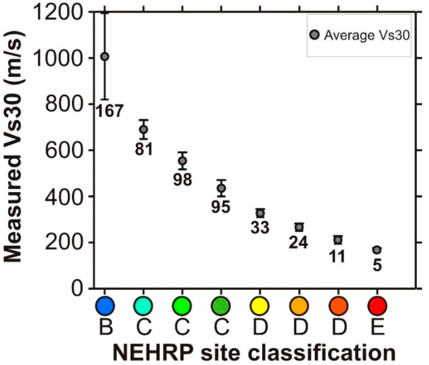
3.1. Vs30 Measurements

Most of the Vs30 data (347 stations out of 514 stations) represent relatively low gradients of less than about 6% ( g r a d e   =   r i s e r u n × 100 ), or a slope of about 3 degrees (angle = arctangent (0.06)). However, in most samples, Vs30 data within ISMN were measured at hard-rock sites rather than the soil sites, implying that slope and Vs30 do not always have a straightforward relationship and must be formulated by applying some constraints, and assigning starting-and-ending values where the data is fewer. Even quite different performance can be expected from rock site measurements [32]. Holzer et al. [14] produced a Vs30 map of San Francisco Bay (140 km2) using Vs30 data of 210 stations, which was derived from (1) the average shear wave velocity values for surficial geologic units, (2) the thickness of each layer, and (3) NEHRP classifications (Table 1). However, it must be considered that in large countries such as Iran (~1.6 million km2), it is difficult to use this approach because it might require a huge pool of Vs30 measurements [33]. The obtained 514 samples do not seem enough to show the significance of the DEM-based Vs30 maps—there is still significant scatter. The regression trend is considered sufficient to be used between gradient of topography and Vs30. Figure 2 shows the statistical results of Vs30 measurements in different NEHRP classes. The number of stations in category B with higher velocities (>760 m/s) is considerably higher than the other classes. Moreover, Tthe standard deviation of this category is high, but in the other classes, it becomes smaller by reducing Vs30.

3.2. SRTM 30c and ASTER 1c

For topography, we considered two types of either low-resolution (SRTM 30c) or medium-resolution (ASTER 1c) elevation data. The SRTM contains the following two radars: (1) the C-band ( λ   =   5.6   c m ) Imaging Radar, and (2) the X-Band ( λ   =   3.0   c m ) Synthetic Aperture Radar sensors, indicating the elevation values between DSM (Digital Surface Model) and DTM (Digital Terrain Model). They were used on board the space shuttle for gathering data about the Earth’s environment with different spatial accuracies (30, 90, and 1000 m). Wald and Allen [15] used SRTM 30c for rather global-purpose Vs30 maps. We used SRTM 30c for the country, freely available by USGS (http://dds.cr.usgs.gov/srtm/version2_1/SRTM30//srtm30). The ASTER sensor gathers data in 14 spectral bands. ASTER 1arcsec is composed of 22,600 tiles, and in this research, over 300 ASTER GeoTIFF tiles (1°×1°) were obtained and merged (http://gdem.ersdac.jspacesystems.or.jp). The key difference between the two datasets is that although ASTER 1c benefits from a stereo imagery technique which gives it the unique ability to create digital elevation models with better accuracy, but the elevations from ASTER sensor constitute a mostly surficial model, whereas SRTM 30c is an interferometry-based elevation model (Allen and Wald, 2007 [15]). Neither SRTM 30c nor ASTER 1c will completely satisfy the topographic gradient of the near surface geology, rather, a bare-ground elevation model will better suit our application. However, owing to the semiarid and arid climate and short vegetation of the study area, the SRTM 30c and ASTER 1c are ideal for slope classification [34]. Note that different resolution topographic data result in different slope values; therefore, some pixel-based resizing can be applied before Vs30 comparison.

4. Vs30 Proxy Map

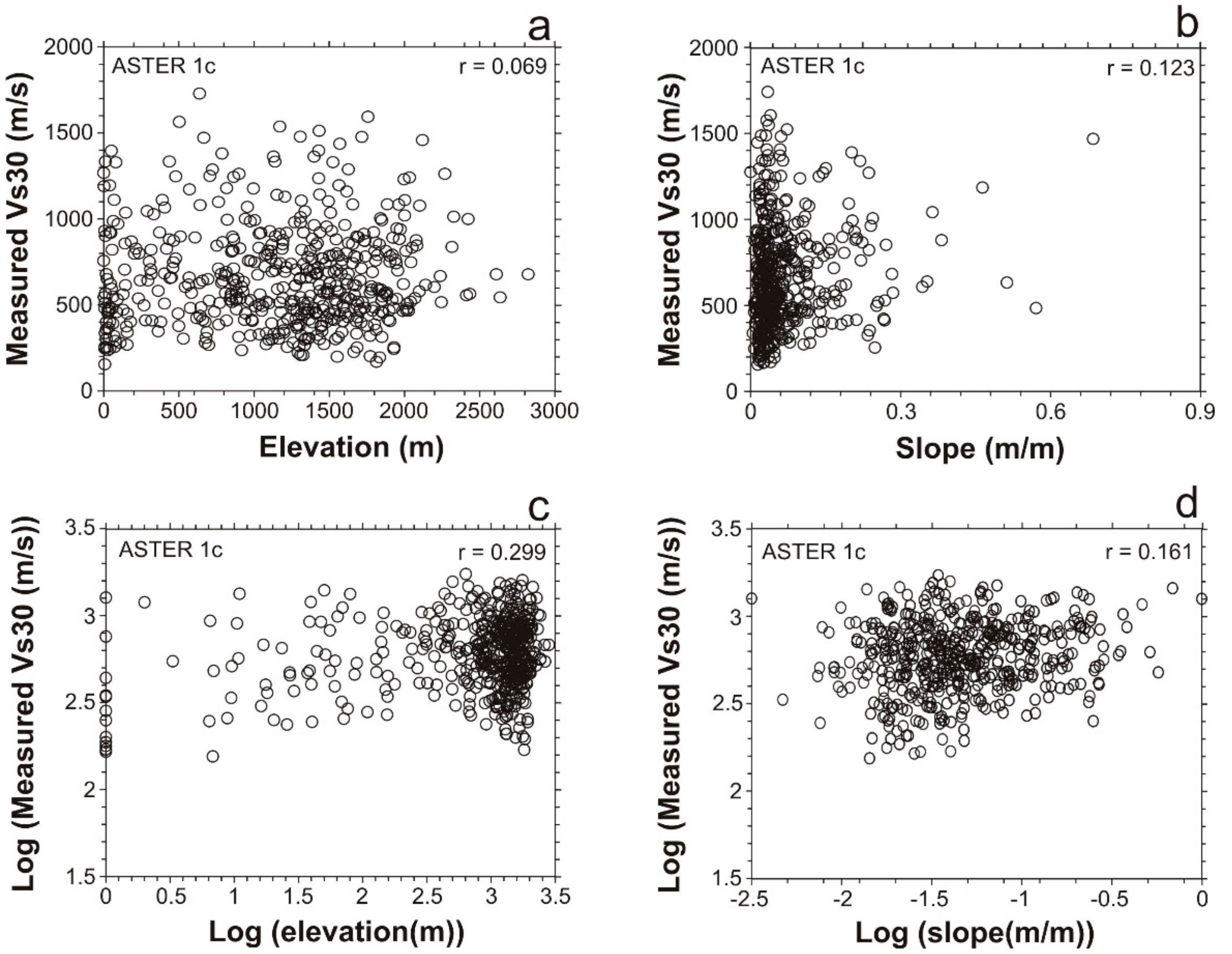
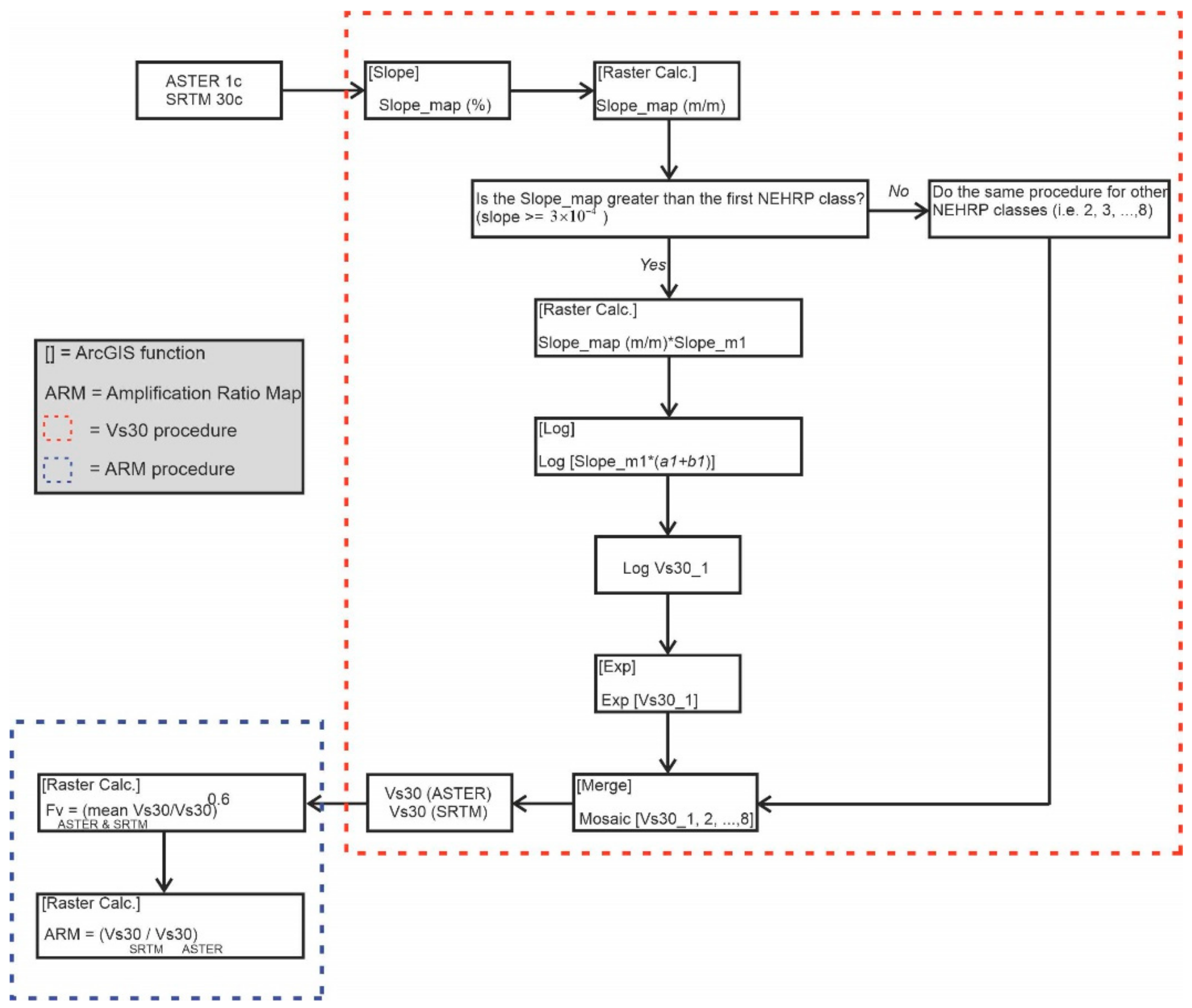
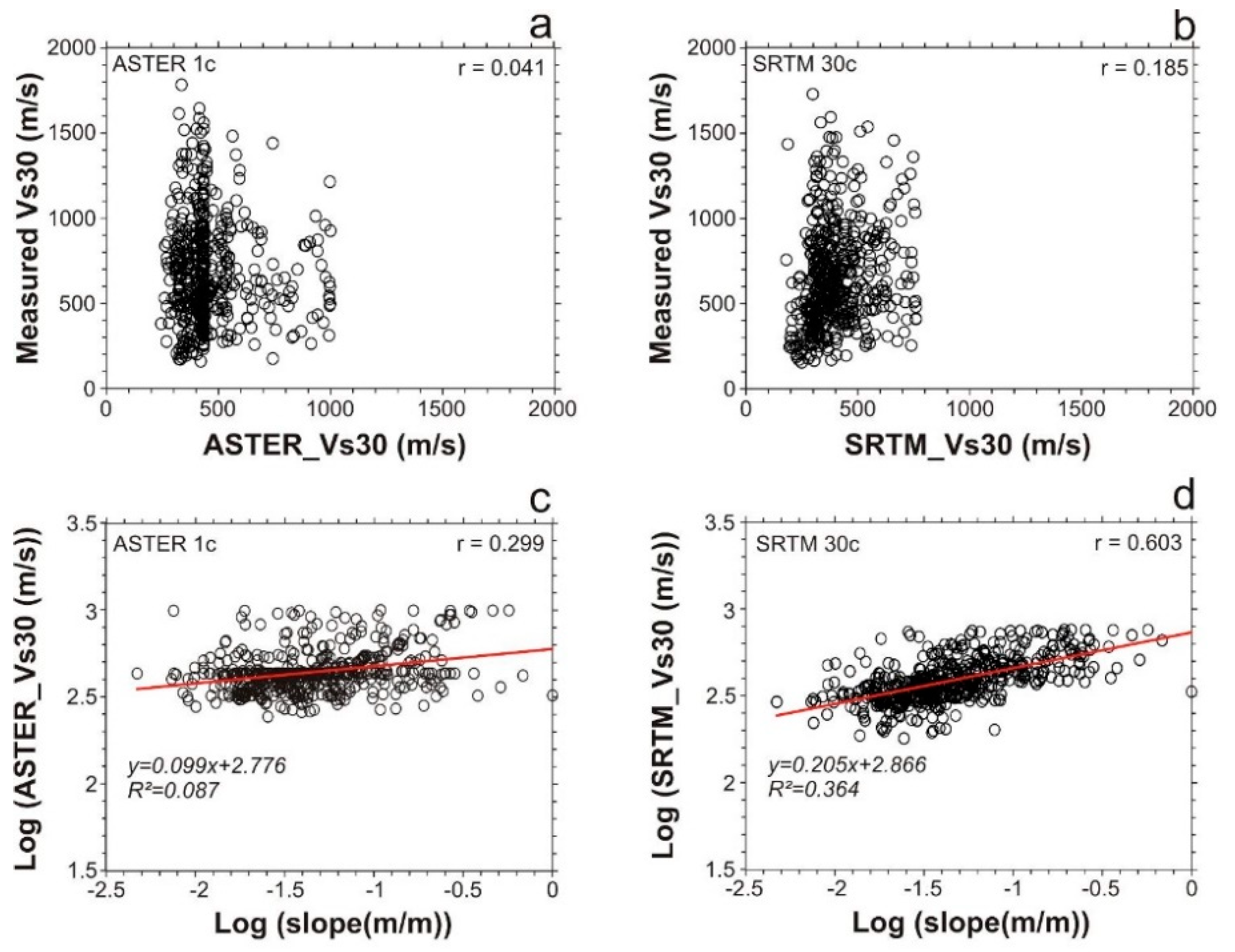
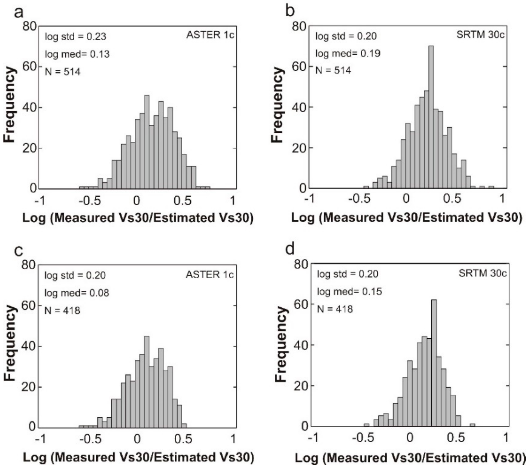
4.1. Regression Analysis and Vs30 Estimation

As the first step of research methodology, topographic attributes (i.e., elevation and slope of topography) were derived and compared with Vs30 data before applying the relevant regression analysis. Every pixel in the output raster (slope map) has a grade slope value ( g r a d e   =   r i s e r u n × 100 ) as a unitless ratio (meter per meter). The lowest slope value represents the flattest terrain and conversely, the highest one represents the steepest ground. The existence of a linear correlation between real Vs30 measurements and topographic attributes at the location of each station is the main concept before the regression analysis, irrespective of whether topographic attributes are useful in the creation of the site condition map or not. Here, the correlation of the variables was examined in both ordinary and logarithmic manners (Figure 3). As shown in Figure 3, the logarithmic correlation between Vs30 and the topographic data is better reflected than the simple correlation between them. The correlation between the height values and Vs30 measurements is too small in comparison with the slope values and the Vs30 measurements (Figure 3a). The slope of the topography describes the relief of the land using a percentage of change over a specified distance. After examining the ASTER 1c data, we noticed that some flat areas have height values near zero. Since the log (0) is not defined, we manually assigned a 1 m pixel value for flat areas. Figure 3b,d manifests that higher Vs30 measurements are in good agreement with the higher slope positions, which is likely related with the competent materials in such higher positions.
Three assumptions are needed before the regression analysis: (1) A logarithmic correlation between the height and the slope with Vs30 measurements should exist. This is essential to perform an independent or joint regression analysis to yield an acceptable outcome. Here, we are only considering slope values since elevation values near zero could be problematic in several ways. (2) We assign a unique Vs30 value (199.06 m/s) for the slope values near to zero in Equation (1). (3) the Vs30 of 600 m/s is assigned to water-covered areas, but inland water bodies can be masked as an alternative option. The regression model of Vs30 and slope is as follow:
log v s 30   =   a × ( log S l o p e ) + b
where a and b are the coefficients of regression analysis for NEHRP classification. For each NEHRP class, the corresponding regression coefficient obtained from a different slope range is given in Table 2, which shows that the coefficient of determination for the areas with a gentle slope is better estimated. This indicates that the database of Wald and Allen [15] was formed from mainly flat sites with relatively lower Vs30 values. Differently from Wald and Allen [15] and Allen and Wald [16], most of the Vs30 measurements in this study are more than 800 m/s, demonstrating that the seismic sites are probably chosen in rock sites (Figure 2).

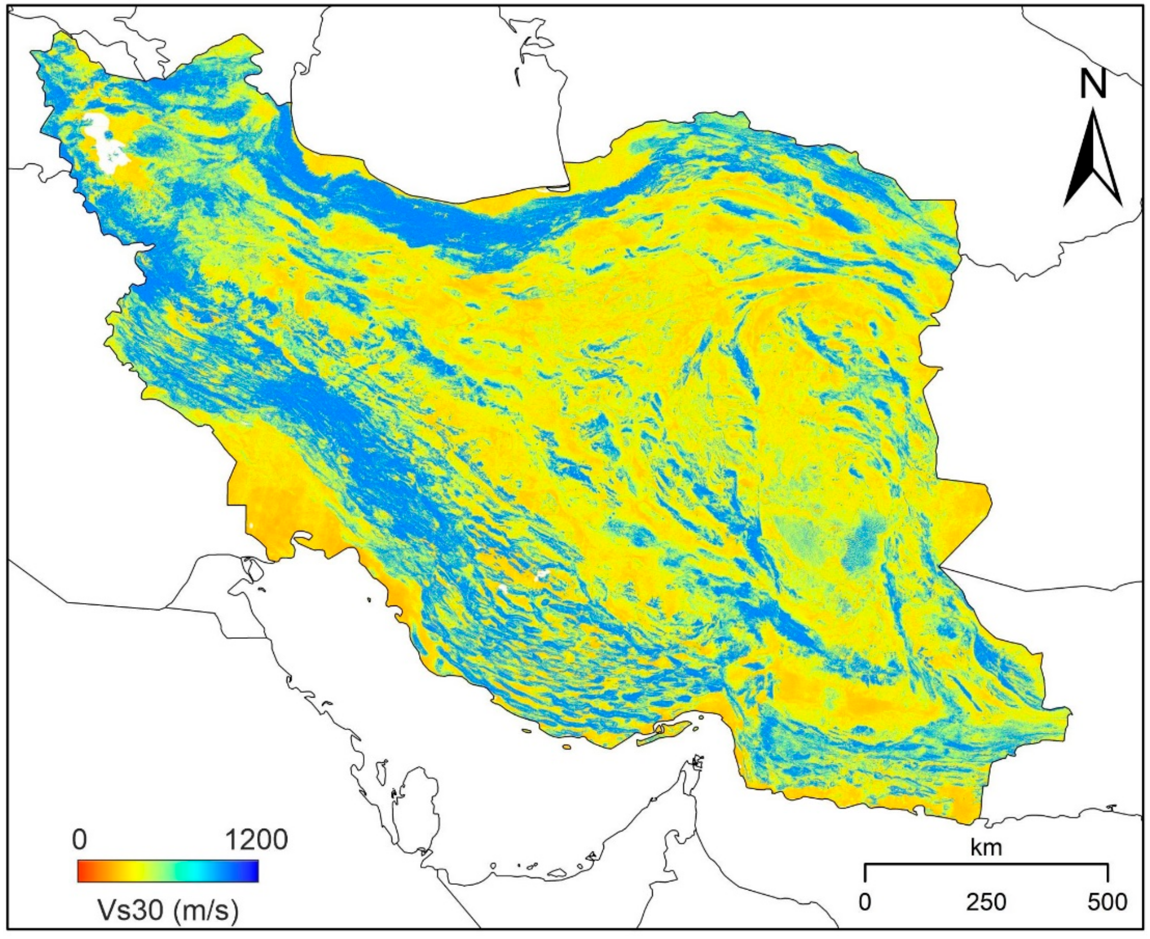
4.2. Vs30 and Amplifiation Map
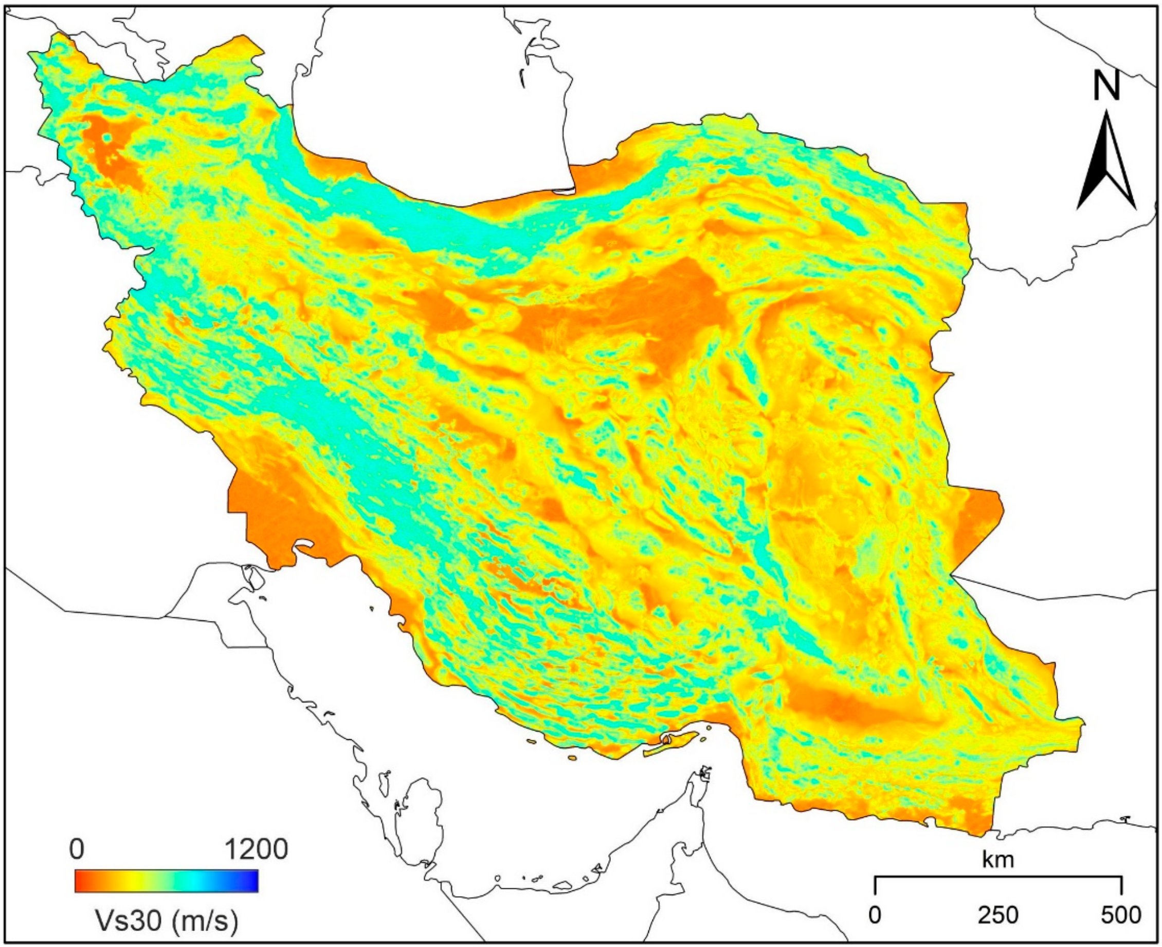
Raster calculation flow allows us to execute mathematical calculations, set up selection queries, and build a model. Once the relationship between regression coefficients and slope ranges is established, the Vs30 map of the country can be estimated [35]. The unitless slope values were assigned to each pixel according to the NEHRP classification (Table 2). As soon as we choose a specific range of slope values in the Raster Calculator tool, all pixels will be rated 0 (unacceptable) or 1 (acceptable), which means that the original values will be lost in the new binary map. One way to recover original pixel value for each class is to multiply the binary map and original map again. Using this method, we were able to recover the real values estimated from ASTER 1c and SRTM 30c slope classes while 0 values remained for void pixels.
Wald et al. [36], following Wald and Allen [15] more fully, described a methodology of a global-based Vs30 grid map from SRTM 30c with larger cells with dimensions of about 0.008 × 0.008 . But the size of each grid of Vs30 values from ASTER 1c was 0.001 × 0.001 . In order to compare new and previous results, their grid sizes must be equal. Thus, we applied the raster generalization to either clean up small erroneous cells or smooth out unnecessary details. We produced 8 discrete classes of the Vs30 map, which should be mosaicked. This procedure tends to produce a very large raster dataset; however, the generalized map along with mosaicking, allow us to take all the raster datasets and combine them into a single, seamless raster dataset between 8 adjacent raster datasets [35]. Nevertheless, there are some overlaps of the raster dataset edges that are being mosaicked together. These overlapping areas have been solved using a weight-based algorithm. Figure 4 and Figure 5 show Vs30 maps deduced from the log slope and the regression coefficients (Table 2).
Next, the amplification map of the study area was calculated using the method suggested by Borcherdt [38]:
  F v = v ¯ v m v
where F v is the amplification factor, v ¯ represents the average value of the shear wave velocity for different sites, v is an individual shear wave velocity in each cell or pixel, and m v is the constant for the corresponding ground motion. Here, Equation (2) has the flexibility to adopt different methods to yield both input ground motion and amplification factors. We calculated the amplification map for midperiods of ground motion by assuming a uniform peak ground acceleration. We took the ratio of the two maps (i.e., Vs30_30c and Vs30_1c) to examine the relative difference in amplification of specific parts of NW Iran (Figure 6). The calculation flow for the Vs30 and amplification ratio maps derived from slope classes is summarized in Figure 7.

4.3. Vs30 Results

The results from the regression analysis and raster calculation indicate that the estimated Vs30 values from SRTM 30c and ASTER 1c can be compared with the ground measurements. At first glimpse, the Vs30 measurements in Iran correlate better with 30c than 1c gradients (Figure 8). The reason for the better correlation between Vs30 from the coarser topography and real Vs30 values is complex, but it seems that it is because of nongeomorphic features. The scatter plots of Vs30 versus Vs30_1c and Vs30 versus log (slope_1c) do not show significant trends (Figure 8a,c). Figure 8 summarizes the trends that we could find from SRTM 30c and ASTER 1c. The overall trend indicates that higher velocities from either ASTER 1c or SRTM 30c are underestimated, mainly because most of the Vs30 data used by Wald and Allen [15] represent relatively low gradients of less than about 7%. Overall, the higher-resolution datasets had better estimation relative to SRTM 30c data. Figure 9a represents the obtained histograms of ASTER 1c for comparison with those produced from SRTM 30c (Figure 9b). The computed logarithmic standard deviation from ASTER 1c (0.23) was larger than that calculated from SRTM 30c (0.20), but the logarithmic median of the first one was smaller than the second, which was a better correlation between the measured and estimated values. The ratio of measured Vs30 and estimated Vs30 is compared for both ASTER 1c and SRTM 30c maps in Figure 8a,b.

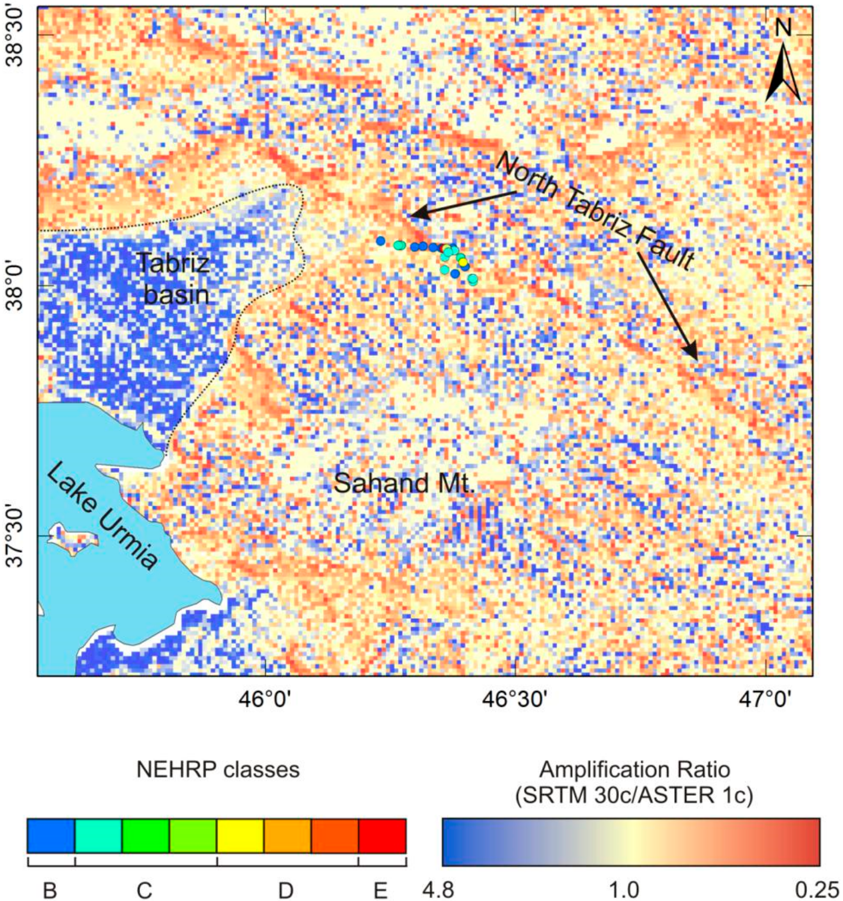
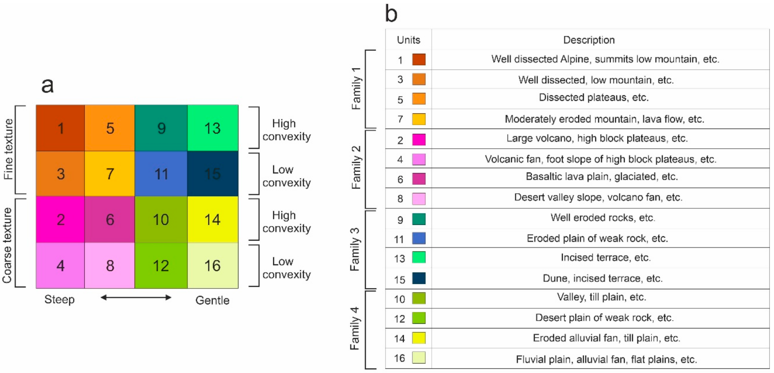
5. Terrain Classification and Site Characterization

In this study, the terrain classification is referred to as geomorphological classification using elevation data. We followed an automated scale-dependent technique developed by Iwahashi and Pike that considers “geometric signature” as a tool of numerical terrain classification [39]. The three components used in the above-mentioned classification method are as follows: slope gradient, surface texture, and local convexity. The slope gradient described in Section 3 is a comprehensive element that describes the surficial processes. Iwahashi and Pike believed that the presence of slope gradient component is enough to describe the elevation. This meant that in the terrain classification process, mere elevation data were not included [39]. Surface texture as a second element was extracted from the ASTER 1c DEM too. The term “texture” indicates the coarseness of the surface or grain sizes. For example, fine textures in local areas have more “peaks” and “troughs” while coarse textures are flatter. Here, the statistical noises which are inherent in digital elevation models were reduced using a 3 × 3 median filter. One important contribution of the texture information is that the texture can enrich the slope information extracted from the first element, in which, some lithologies can be differentiated from the others. For instance, local areas located in coarse texture and a planar slope may explain a Quaternary plain. Local convexity as a third element measures convexity of the features in which the value of 1 represents no holes, and the values less than 1 represent concave features. Convexity can be calculated as follow:
c o n v e x t i y   =   l L
where l and L are length of convex hull and Euclidian length, respectively. Positive values are upward convexity and negative values are concave areas. The classification algorithm is able to classify the terrain into 8, 12, and 16 classes. We classified the terrain into 16 classes to have more diverse classes. The description of different geomorphological information is represented in a colored matrix (Figure 10a). Geomorphological descriptions of classes in pixel-based and object-based manners are given in Iwahashi and pike [39] and Iwahashi et al. [40]. However, the pixel-based approach, in some cases (e.g., geomorphological map of Thailand), has shown reliable results [41]. Therefore, we also followed the pixel-based method. Each family of classes had rather the same color and characteristics. For instance, the colors near to pink (units 2, 4, 6, and 8 ((Family 2)) describe volcanic landforms in a pixel-based manner (Figure 10b).

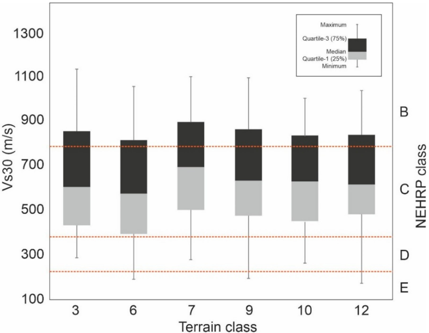
6. Terrain Classification Results

To determine where exactly the seismic stations are constructed, we carried out a geomorphological classification for the whole study area with a 10-pixel window size. It must be noted that we only classified the study area using ASTER 1c because terrain classification in global scale had been done using 90 m and 280 m elevation data in the previous studies [39,40]. The aim was to add more attributes for the existing seismic sites with an affordable DEM-based approach. Unlike the Vs30 regression analysis, we did not assign pre-defined values for water bodies (e.g., lakes, wetlands); these areas were removed from ASTER 1c. The majority of the stations in different seismotectonic zones were categorized as follows:
In the Kopet Dagh zone, eight stations out of 34 were categorized in class 12, in the Alborz-Azarbaijan zone, 24 stations out of 103 were categorized in class 9, in the Lut block, 23 stations out of 55 were categorized in class 6, in the Makran zone, 3 stations out of 7 were categorized in class 12, in the Zagros zone, 72 stations out of 190 were categorized in class 12, and in the Central Iran block, 28 stations out of 124 were categorized in class 12. In addition, the results show that 98% of the stations are situated in six classes 30% of which are in class 12, 27% in class 6, 17% in class 9, 16% in class 3, 4% in class 4, and the rest of the stations are located in other classes (Figure 11). This implies that the stations are not only located in volcanic sites, but also in desert plains of weak rocks. We eliminated other classes with insufficient Vs30 observations and tried to plot only the main six units (3, 6, 7, 9, 10, and 12) versus the measured Vs30 values in Figure 12. Although most of the stations in Figure 12 belong to class C in NEHRP classification, the standard deviation bars for class 3 and 12 have a tendency to the upward NEHRP class (i.e., class D) and the downward NEHRP class (class B). The median value for mountain classes like 3 and 7 is relatively high, whilst for smoother classes like 12, it is relatively low (Figure 12). Intermediate classes like basaltic lava plains also showed lower Vs30 values.

7. Discussion

The regression analysis of Vs30 shows that the correlation between slope and Vs30 values in the Iranian territory is low. The lack of a meaningful trend is not unexpected because sedimentary slopes have a better correlation with Vs30 measurements (Wald and Allen [15]) and most of the stations used in this study are probably constructed in rock slopes. Thus, the lack of correlation in rock units may obscure the trend interpretations. The terrain surface classification also showed that most of the stations were constructed in mountainous or intermediate positions (Figure 12). Generally, this trend is not important because steep hill slopes and ridge positions are not suitable lands for building structures, whereas flat and gentle slopes tend to consist of more fertile soils suitable for inhabitation. Thus, the calculated Vs30 values in lower slopes can be used profitably in the development of damage/loss models. The histogram resulting from the ASTER 1c map shows a wider distribution in the comparison of the observed and estimated Vs30 (Figure 9a). However, unlike most other regions studied by Wald and Allen [15] (e.g., California, Italy, and Taiwan), many of the Iranian sites were constructed on rock, so the distribution is biased toward higher-velocity Vs30 data. Accordingly, the correlation of the measured Vs30 and estimated Vs30 were modified for both ASTER 1c and SRTM 30c maps by ignoring Vs30 data larger than 1000 m/s. The logarithmic median values in the new histograms are now narrower and closer to zero, which means that the misfit between the measured and estimated values for both ASTER 1c and SRTM 30c was reduced (Figure 9c and d), but the standard deviation of the residuals is not significantly improved in SRTM 30c. This procedure shows that the ISMN stations are designed on rock sites to avoid noisy records of accelerometers. Thus, the 514 Vs30 measurements are expected to reflect high Vs30 values. Probably, rock slope is not indicative of Vs30, but the correlation between Vs30 and slope within sediments (e.g., young alluviums) reflects stream power.

8. Conclusions

In this study, we focused on the use of two different digital elevation models with two different resolutions (medium and low resolutions). Although the results of the regression analysis cannot explain the Vs30 measurements perfectly, the combination of ASTER 1c and SRTM 30c amplification maps can be useful in the detection of geological and geomorphological units. For the amplification ratio (SRTM 30c/ASTER 1c) of NW Iran (Figure 6), the blue pixels indicate where the SRTM-based amplification is higher and the red pixels indicate where the ASTER-based amplification is higher. The white-to-yellow pixels represent a similar amplification and are thus commonly related with low gradients. For example, the North Tabriz fault (NW-SE trend) with red pixel values and the Tabriz basin with blue pixel values can be explicitly identified using a combined amplification map (Figure 6). Thus, while medium-resolution DEM is able to delineate the position of small slope changes, low-resolution DEM results in more realistic maps in flat areas.
In addition, the geomorphological analysis showed that under a pre-defined scale or radius, the stations are not only located in volcanic sites, but also in desert plains of weak rocks. However, significant changes in the scale could affect the number of stations in each geomorphological unit. Therefore, the scale should be selected carefully according to the purposes.

Author Contributions

Conceptualization, Sadra Karimzadeh and Masashi Matsuoka; methodology, Sadra Karimzadeh, Masashi Matsuoka and Bakhtiar Feizizadeh; software, Sadra Karimzadeh and Bakhtiar Feizizadeh; validation, Sadra Karimzadeh; formal analysis, Sadra Karimzadeh; investigation, Sadra Karimzadeh; resources, Sadra Karimzadeh, Masashi Matsuoka and Bakhtiar Feizizadeh; data curation, Sadra Karimzadeh; writing—original draft preparation, Sadra Karimzadeh; visualization, Sadra Karimzadeh; supervision, Sadra Karimzadeh and Masashi Matsuoka; project administration, Sadra Karimzadeh, Masashi Matsuoka and Bakhtiar Feizizadeh; funding acquisition, Sadra Karimzadeh, Masashi Matsuoka and Bakhtiar Feizizadeh.

Funding

This study was funded by the National Elites Foundation of Iran at University of Tabriz (No. 102–5146) and the Japan Society for the Promotion of Science (JSPS) Grants-in-Aid for scientific research (KAKENHI) number 16F16380 and 17H02050.

Conflicts of Interest

The authors declare no conflicts of interest.

References

  1. Hassanzadeh, R.; Zorica, N.; Razavi, A.A.; Norouzzadeh, M.; Hodhodkian, H. Interactive approach for GIS-based earthquake scenario development and resource estimation (Karmania hazard model). Comput. Geosci. 2013, 51, 324–338. [Google Scholar] [CrossRef]
  2. Karimzadeh, S.; Miyajima, M.; Hassanzadeh, R.; Amiraslanzadeh, R.; Kamel, B.A. GIS-based seismic hazard, building vulnerability and human loss assessment for the earthquake scenario in Tabriz. Soil Dyn. Earthq. Eng. 2014, 66, 263–280. [Google Scholar] [CrossRef]
  3. Hassanzadeh, R.; Zorica, N. Where to go first: Prioritization of damaged areas for allocation of Urban Search and Rescue (USAR) operations (PI-USAR model). Geomat. Nat. Hazards Risk 2015, 7, 1337–1366. [Google Scholar] [CrossRef]
  4. Matsuoka, M.; Wakamatsu, K.; Fujimoto, K.; Midorikawa, S. Nationwide site amplification zoning using GIS-based Japan Engineering Geomorphologic Classification Map. In Proceedings of the ICOSSAR, Millpress, Bethlehem, PA, USA, 19 June 2005; pp. 239–246. [Google Scholar]
  5. Matsuoka, M.; Wakamatsu, K.; Fujimoto, K.; Midorikawa, S. Average shear-wave velocity mapping using Japan Engineering Geomorphologic Classification Map. J. Struct. Mech. Earthq. Eng. 2006, 23, 57s–68s. [Google Scholar] [CrossRef]
  6. Karimzadeh, S.; Miyajima, M.; Kamel, B.; Pessina, V. A fast topographic characterization of seismic station locations in Iran, through integrated use of Digital Elevation Models and GIS. J. Seismol. 2015, 19, 949–967. [Google Scholar] [CrossRef]
  7. Karimzadeh, S. Characterization of land subsidence in Tabriz basin (NW Iran) using InSAR and watershed analyses. Acta Geod. Geophys. 2015, 51, 181–195. [Google Scholar] [CrossRef]
  8. Iwahashi, J.; Kamiya, I.; Matsuoka, M. Regression analysis of Vs30 using topographic attributes from a 50-m DEM. Geomorphology 2010, 117, 202–205. [Google Scholar] [CrossRef]
  9. Lemoine, A.; Douglas, J.; Cotton, F. Testing the Applicability of Correlations between Topographic Slope and Vs30 for Europe. Bull. Seismol. Soc. Am. 2012, 102, 2585–2599. [Google Scholar] [CrossRef]
  10. Burjanek, J.; Edwards, B.; Fah, D. Empirical evidence of local seismic effects at sites with pronounced topography: A systematic approach. Geophys. J. Int. 2014, 197, 608–619. [Google Scholar] [CrossRef]
  11. Kwok, A.; Chiu, H. Developing correlation relationships of Vs30 for use in site classification in Taiwan. In Proceedings of the Tenth US National Conference on Earthquake Engineering Frontiers of Earthquake Engineering, Alaska, AK, USA, 21–25 July 2014. [Google Scholar]
  12. Wills, C.J.; Petersen, M.D.; Bryant, W.A.; Reichle, S.; Saucedo, G.J.; Tan, S.S.; Taylor, G.C.; Treiman, J.A. A site conditions map for California based on geology and shear wave velocity. Bull. Seismol. Soc. Am. 2000, 90, S187–S208. [Google Scholar] [CrossRef]
  13. Kawase, H. Site effects on strong ground motions. In International Handbook of Earthquake and Engineering Seismology; Academic Press: New York, NY, USA, 2003; pp. 1013–1030. [Google Scholar]
  14. Holzer, T.L.; Padovani, A.C.; Bennett, M.J.; Noce, T.E.; Tinsley, J.C. Mapping NEHRP VS30 site classes. Earthq. Spectra 2005, 2, 353–370. [Google Scholar] [CrossRef]
  15. Wald, D.J.; Allen, T.I. Topographic slope as a proxy for seismic site conditions and amplification. Bull. Seismol. Soc. Am. 2007, 97, 1379–1395. [Google Scholar] [CrossRef]
  16. Allen, T.I.; Wald, D.J. On the Use of High-Resolution Topographic Data as a Proxy for Seismic Site Conditions (VS30). Bull. Seismol. Soc. Am. 2009, 99, 935–943. [Google Scholar] [CrossRef]
  17. Allen, T.I.; Wald, D.J. Topographic Slope as a Proxy for SeismicSite-Conditions (VS30) and Amplification around the Globe; Open-File Report, 1357 U.S.; Geological Survey Reston: Virginia, VA, USA, 2007. [Google Scholar]
  18. Chung, J.W.; Rogers, D. Seismic Site Classifications for the St. Louis Urban Area. Bull. Seismol. Soc. Am. 2012, 102, 980–990. [Google Scholar] [CrossRef]
  19. Iranian Code of Practice for Seismic Resistance Design of Buildings, 4th ed.; Iranian building codes and standards, standard no. 2800; Building and Housing Research Center (BHRC): Tehran, Iran, 2014.
  20. NEHRP Recommended Seismic Provisions for New Buildings and Other Structures Volume I: Part 1 Provisions, Part 2 Commentary FEMA; A council of the National Institute of Building Sciences: Washington, DC, USA, 2015.
  21. Matsuoka, M.; Yamamoto, N. Web-based Quick Estimation System of Strong Ground Motion Maps Using Engineering Geomorphologic Classification Map and Observed Seismic Records. In Proceedings of the 15th World Conference on Earthquake Engineering, Portuguese Association for Earthquake Engineering, Lisbon, Portugal, 24–28 September 2012; p. 10. [Google Scholar]
  22. Forte, G.; Chioccarelli, E.; De Falco, M.; Cito, P.; Santo, A.; Iervolino, I. Seismic soil classification of Italy based on surface geology and shear-wave velocity measurements. Soil Dyn. Earthq. Eng. 2019, 122, 79–93. [Google Scholar] [CrossRef]
  23. Stewart, J.P.; Klimis, N.; Savvaidis, A.; Theodoulidis, N.; Zargli, E.; Athanasopoulos, G.; Pelekis, P.; Mylonakis, G.; Margaris, B. Compilation of a local vs. profile database and its application for inference of VS30 from geologic- and terrain-based proxies. Bull. Seismol. Soc. Am. 2014, 104, 2827–2841. [Google Scholar] [CrossRef]
  24. Yong, A. Comparison of measured and proxy-based VS30 values in California. Earthq. Spectra 2016, 32, 171–192. [Google Scholar] [CrossRef]
  25. Vernant, P.; Nilforoushan, F.; Hatzfeld, D.; Abbassi, M.R.; Vigny, C.; Masson, F.; Nankali, H.; Martinod, J.; Ghafory-Ashtiany, M.; Bayer, R.; et al. Present-Day Crustal Deformation and Plate Kinematics in the Middle East Constrained by GPS Measurements in Iran and Northern Oman. Geophys. J. Int. 2004, 157, 381–398. [Google Scholar] [CrossRef]
  26. Nowroozi, A.A. Seismotectonic provinces of Iran. Bull. Seismol. Soc. Am. 1976, 66, 1249–1276. [Google Scholar]
  27. Berberian, M. Discussion of the paper A.A. Nowroozi, 1976 “Seismotectonic provinces of Iran”. Bull. Seismol. Soc. Am. 1979, 69, 293–297. [Google Scholar]
  28. Mirzaei, N.; Mengtan, G.; Yantai, C. Seismic source regionalization for seismic zoning of Iran: Major seismotectonic provinces. J. Earthq. Predict. Res. 1998, 7, 465–495. [Google Scholar]
  29. Mojarab, M.; Memarian, H.; Zare, M.; Morshedy, A.H.; Pishahang, M.H. Modeling of the seismotectonic provinces of Iran using the self-organizing map algorithm. Comput. Geosci. 2014, 67, 150–162. [Google Scholar] [CrossRef]
  30. Yazdani, A.; Kowsari, M. Bayesian estimation of seismic hazards in Iran. Sci. Iran. 2013, 20, 422–430. [Google Scholar]
  31. Mirzaei, H.; Farzanegan, E. Iran Strong Motion Network (Technical Note). Asian J. Civ. Eng. Build. Hous. 2003, 4, 173–186. [Google Scholar]
  32. Mousavi, M.; Zafarani, H.; Rahpeyma, S.; Azarbakht, A. Test of Goodness of the NGA Ground-Motion Equations to Predict the Strong Motions of the 2012 Ahar–Varzaghan Dual Earthquakes in Northwestern Iran. Bull. Seismol. Soc. Am. 2014, 104, 2512–2528. [Google Scholar] [CrossRef]
  33. Wills, C.J.; Clahan, K.B. Developing a map of geologically defined site-condition categories for California. Bull. Seismol. Soc. Am. 2006, 96, 1483–1501. [Google Scholar] [CrossRef]
  34. Nikolakopoulos, K.G.; Kamaratakis, E.K.; Chrysoulakis, N. SRTM vs. ASTER elevation products. Comparison for two regions in Crete, Greece. Int. J. Remote Sens. 2006, 27, 4819–4838. [Google Scholar] [CrossRef]
  35. Raster Tutorial; ESRI: Redlands, CA, USA, 2010; pp. 8–21. Available online: http://help.arcgis.com/en/arcgisdesktop/10.0/pdf/raster-tutorial.pdf (accessed on 01 October 2018).
  36. Wald, D.J.; Earle, P.S.; Quitoriano, V. Topographic Slope as a Proxy for Seismic Site Correction and Amplification. EOS Trans AGU 2004, 85, F1424. [Google Scholar]
  37. Karimzadeh, S.; Feizizadeh, B.; Matsuoka, M. From a GIS-based hybrid site condition map to an earthquake damage assessment in Iran: Methods and trends. Int. J. Disaster Risk Reduct. 2017, 22, 23–36. [Google Scholar] [CrossRef]
  38. Borcherdt, R.D. Estimates of site-dependent response spectra for design (methodology and justification). Earthq. Spectra 1994, 10, 617–653. [Google Scholar] [CrossRef]
  39. Iwahashi, J.; Pike, R.J. Automated classification of topography from DEMs by an unsupervised nested-means algorithm and a three-part geometric signature. Geomorphology 2007, 86, 409–440. [Google Scholar] [CrossRef]
  40. Iwahashi, J.; Kamiya, I.; Matsuoka, M.; Yamazaki, D. Global terrain classification using 280 m DEMs: Segmentation, clustering, and reclassification. Prog. Earth Planet. Sci. 2018, 5, 1. [Google Scholar] [CrossRef]
  41. Thamarux, P.; Matsuoka, M.; Poovarodom, N.; Iwahashi, J. VS30 Seismic Microzoning Based on a Geomorphology Map: Experimental Case Study of Chiang Mai, Chiang Rai, and Lamphun, Thailand. ISPRS Int. J. Geo-Inf. 2019, 8, 309. [Google Scholar] [CrossRef] [Green Version]
Figure 1. Map of Iran showing 6 seismotectonic regions. The circles indicate the location of 514 strong motion seismometer stations with their color-coded Vs30 measurements (m/s).
Ijgi 08 00537 g001
Figure 2. Mean value and standard deviation (error bars) of Vs30 measurements based on NEHRP classification.
Ijgi 08 00537 g002
Figure 3. Scatter plots of measured Vs30 versus ASTER 1c topographic attributes for (a) elevation (m) and (b) slope (m/m); log Vs30 versus (c) log elevation (m) and (d) log slope (m/m). The correlation coefficient is given in the upper right corner of each panel, indicating that logarithmic data have a better correlation with the topographic attributes.
Ijgi 08 00537 g003
Figure 4. Vs30 map of Iran based on ASTER 1c and a regression analysis.
Ijgi 08 00537 g004
Figure 5. Vs30 map of Iran based on SRTM 30c from Wald and Allen [15].
Ijgi 08 00537 g005
Figure 6. The combined amplification map of NW Iran (STRM 30c amplification/ASTER 1c amplification), based on the Borcherdt [38] amplification factors. North Tabriz fault (NW-SE trend) with red pixel values and Tabriz basin with blue pixel values can be explicitly identified using a combined amplification map. The blue pixels indicate where the SRTM-based amplification is higher and the red pixels indicate where the ASTER-based amplification is higher. In the white-to-yellow pixels, the amplification is almost the same between the two amplification maps. The colored circles are local Vs30 measurements in Tabriz city.
Ijgi 08 00537 g006
Figure 7. Vs30 and amplification ratio estimation model.
Ijgi 08 00537 g007
Figure 8. (a) and (b) are scatter plots of measured Vs30 versus estimated Vs30 derived from ASTER 1c and STRM 30c, respectively; (c) and (d) are also scatter plots of log Vs30 versus log slope. The regression lines and R2 values in (c) and (d) indicate the extent of the predictable variance from the independent variables.
Ijgi 08 00537 g008
Figure 9. (a) and (b) are histograms describing logarithmic differences of measured Vs30 values versus Vs30 values derived from ASTER 1c and SRTM 30c, respectively; (c) and (d) are histograms describing logarithmic differences of modified Vs30 values versus Vs30 values derived from ASTER 1c and SRTM 30c, respectively.
Ijgi 08 00537 g009
Figure 10. (a) Morphological matrix defined by Iwahashi and Pike [39]; (b) description of terrain units.
Ijgi 08 00537 g010
Figure 11. Morphological classification map of Iran.
Ijgi 08 00537 g011
Figure 12. Boxplot of some terrain classes and the extracted Vs30 values at the location of 514 stations.
Ijgi 08 00537 g012
Table 1. Topographic slope ranges for NEHRP classes adopted by Allen and Wald [16].
NEHRP Site ClassificationVs30 Range (m/s)Slope Range (m/m)General Description
Active Tectonic RegionsCraton Regions
E < 180 < 3 × 10 4 < 1 × 10 4 Soil profile with soft clay
D 180 240 3 × 10 4 3.5 × 10 3 1 × 10 4 8.5 × 10 3 Stiff soil
D 240 300 3.5 × 10 3 0.010 4.5 × 10 3 8.5 × 10 3 Stiff soil
D 300 360 0.010 0.024 8.5 × 10 3 0.013 Stiff soil
C 360 490 0.024 0.08 0.013 0.022 Very dense soil and soft rock
C 490 620 0.08 0.14 0.022 0.03 Very dense soil and soft rock
C 620 760 0.14 0.20 0.03 0.40 Very dense soil and soft rock
B > 760 > 0.20 > 0.40 Rock & Hard rock
Table 2. Corresponding coefficients for active regions compatible with NEHRP slope classes [37].
Slope Range (m/m)Vs30 Range (m/s) log v s 30   =   a × ( log S l o p e ) + b R 2
a b
< 3 × 10 4 < 180 0.46 2.229 0.136
3 × 10 4 3.5 × 10 3 180 240 0.18 2.293 0.008
3.5 × 10 3 0.010 240 300 0.12 2.443 0.025
0.010 0.024 300 360 0.12 2.531 0.035
0.024 0.08 360 490 0.001 2.638 0.000
0.08 0.14 490 620 0.003 2.747 0.002
0.14 0.20 620 760 0.002 2.841 0.001
> 0.20 > 760 0.006 3.001 0.000

