A Multilevel Eigenvector Spatial Filtering Model of House Prices: A Case Study of House Sales in Fairfax County, Virginia


Abstract
1. Introduction
2. Background
3. Materials and Methods
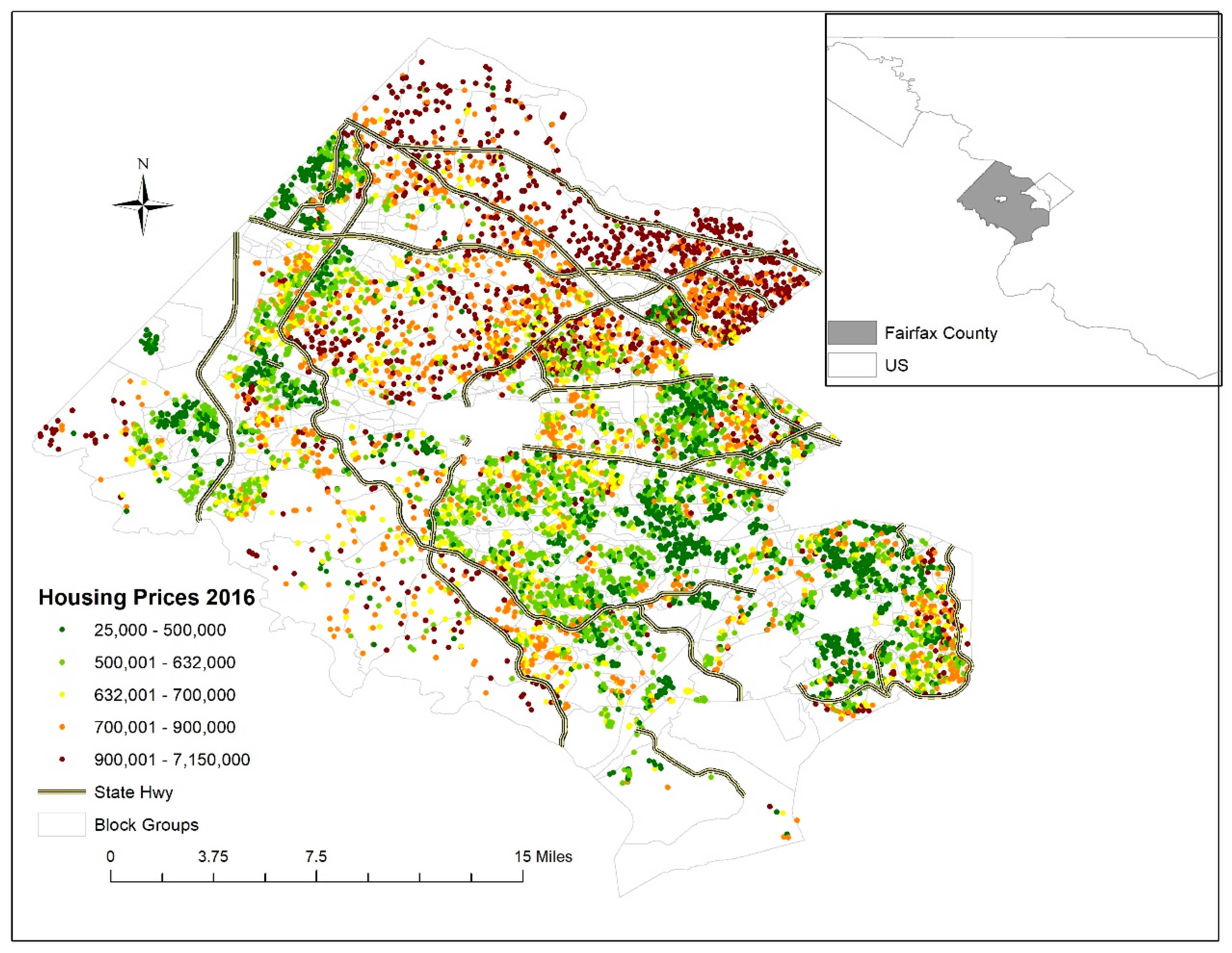
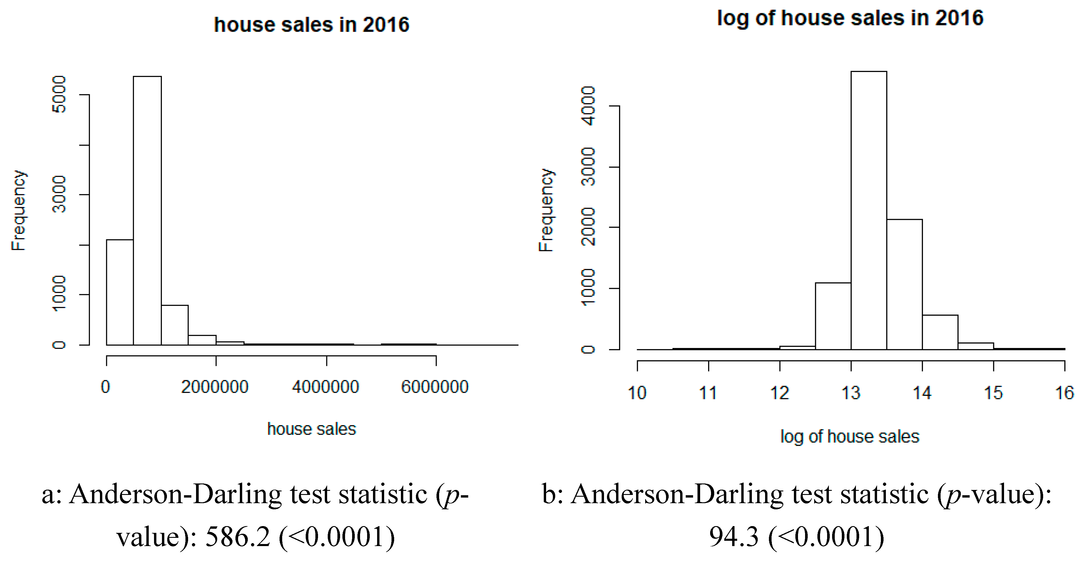
3.1. Data and Variables
3.2. Model Specifications
4. Results
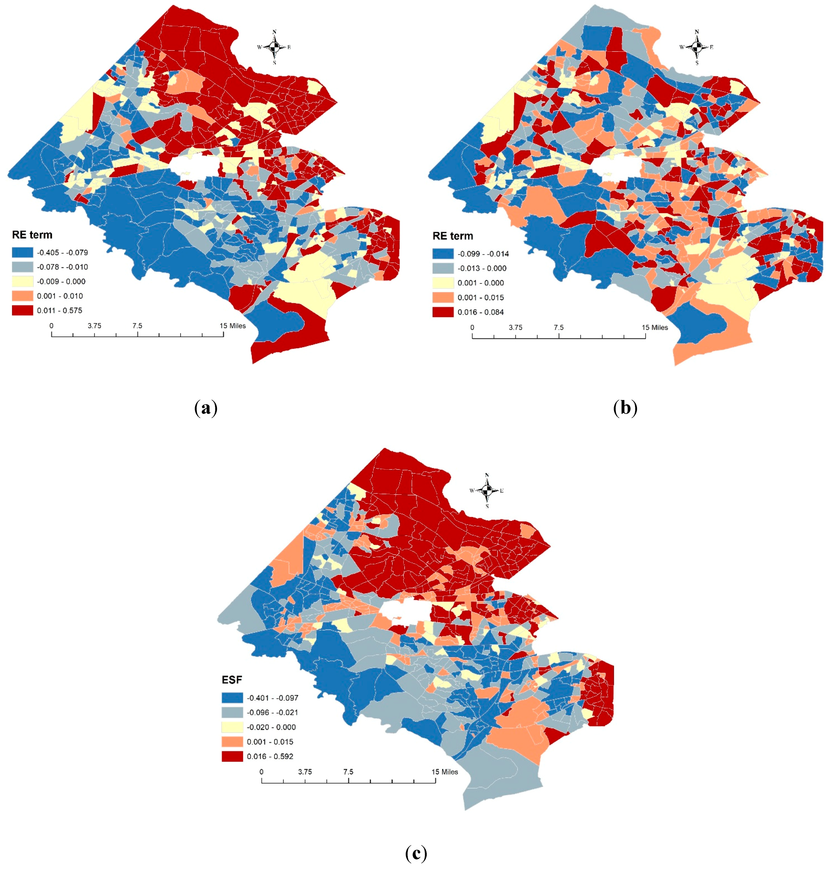
4.1. Regression Results
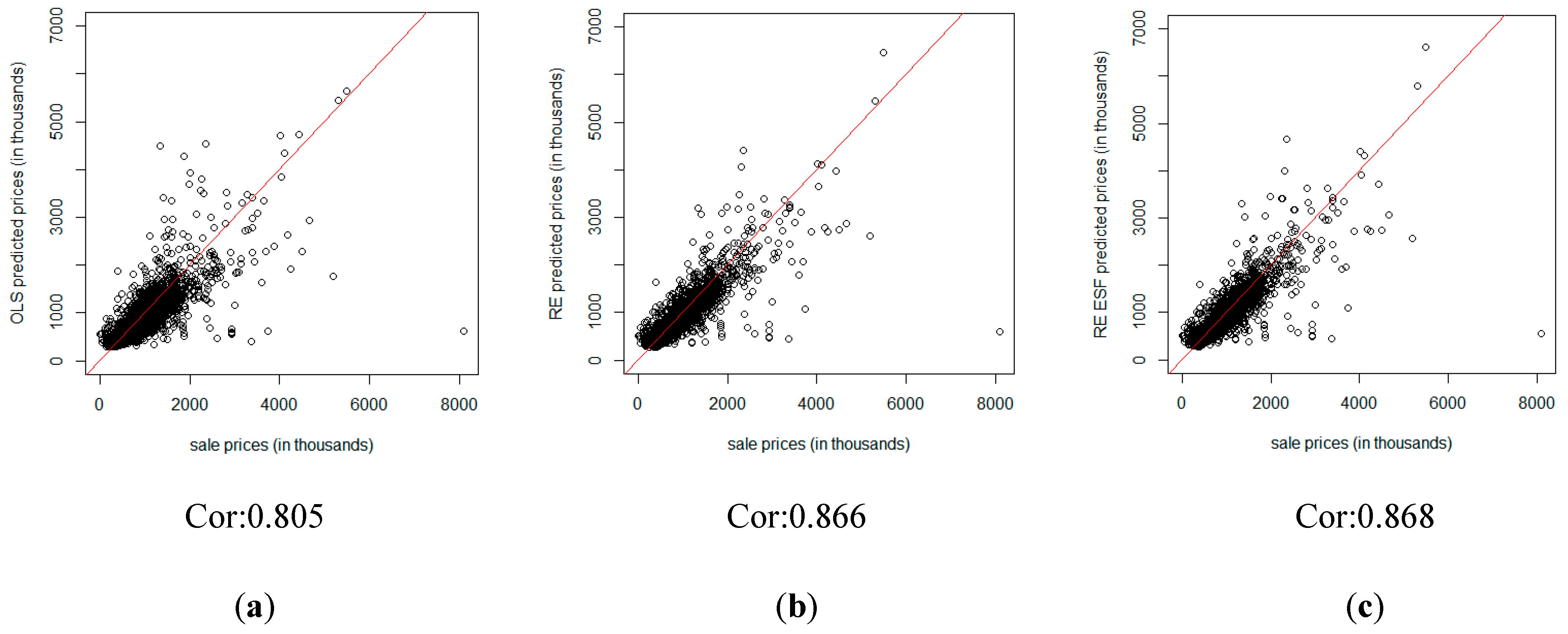
4.2. A House Price Prediction Analysis
5. Discussion
6. Conclusions
Author Contributions
Funding
Conflicts of Interest
References
- Basu, S.; Thibodeau, T.G. Analysis of spatial autocorrelation in house prices. J. Real Estate Financ. Econ. 1998, 17, 61–85. [Google Scholar] [CrossRef]
- Cohen, J.P.; Coughlin, C.C. Spatial hedonic models of airport noise, proximity, and housing prices. J. Reg. Sci. 2008, 48, 859–878. [Google Scholar] [CrossRef]
- Pace, R.K.; Barry, R.; Clapp, J.M.; Rodriquez, M. Spatiotemporal autoregressive models of neighborhood effects. J. Real Estate Financ. Econ. 1998, 17, 15–33. [Google Scholar] [CrossRef]
- Bitter, C.; Mulligan, G.F.; Dall’erba, S. Incorporating spatial variation in housing attribute prices: A comparison of geographically weighted regression and the spatial expansion method. J. Geogr. Syst. 2007, 9, 7–27. [Google Scholar] [CrossRef]
- Huang, B.; Wu, B.; Barry, M. Geographically and temporally weighted regression for modeling spatio-temporal variation in house prices. Int. J. Geogr. Inf. Sci. 2010, 24, 383–401. [Google Scholar] [CrossRef]
- Chica-Olmo, J. Prediction of house location price by a multivariate spatial method: Cokriging. J. Real Estate Res. 2007, 29, 91–114. [Google Scholar]
- Dubin, R.A. Spatial autocorrelation and neighborhood quality. Reg. Sci. Urban Econ. 1992, 22, 433–452. [Google Scholar] [CrossRef]
- Gámez Matínez, M.; Montero Lorenzo, J.M.; García Rubio, N. Kriging methodology for regional economic analysis: Estimating the housing price in Albacete. Int. Adv. Econ. Res. 2000, 6, 438–451. [Google Scholar] [CrossRef]
- Djurdjevic, D.; Eugster, C.; Haase, R. Estimation of hedonic models using a multilevel approach: An application for the Swiss rental market. Swiss J. Econ. Stat. 2008, 144, 679–701. [Google Scholar] [CrossRef]
- Chasco, C.; Le Gallo, J. Hierarchy and spatial autocorrelation effects in hedonic models. Econ.Bull. 2012, 32, 1474–1480. [Google Scholar]
- Orford, S. Modelling spatial structures in local house market dynamics: A multilevel perspective. Urban Stud. 2000, 37, 1643–1671. [Google Scholar] [CrossRef]
- Chaix, B.; Merlo, J.; Chauvin, P. Comparison of a spatial approach with the multilevel approach for investigating place effects on health: The example of healthcare utilisation in France. J. Epidemiol. Community Health 2005, 59, 517–526. [Google Scholar] [CrossRef] [PubMed]
- Can, A. Specification and estimation of hedonic house price models. Reg. Sci. Urban Econ. 1992, 22, 453–474. [Google Scholar] [CrossRef]
- Laurice, J.; Bhattacharya, R. Prediction performance of a hedonic pricing model for house. Apprais. J. 2005, 73, 198. [Google Scholar]
- Limsombunchai, V. House Price Prediction: Hedonic Price Model vs. Artificial Neural Network. In Proceedings of the New Zealand Agricultural and Resource Economics Society Conference, Blenheim, New Zealand, 25–26 June 2004; pp. 25–26. [Google Scholar]
- Liu, X. Spatial and temporal dependence in house price prediction. J. Real Estate Financ. Econ. 2013, 47, 341–369. [Google Scholar] [CrossRef]
- Leishman, C.; Costello, G.; Rowley, S.; Watkins, C. The predictive performance of multilevel models of house sub-markets: A comparative analysis. Urban Stud. 2013, 50, 1201–1220. [Google Scholar] [CrossRef]
- Bourassa, S.C.; Hoesli, M.; Peng, V.C. Do house submarkets really matter? J. House Econ. 2003, 12, 12–28. [Google Scholar] [CrossRef]
- Goodman, A.C.; Thibodeau, T.G. House market segmentation and hedonic prediction accuracy. J. House Econ. 2003, 12, 181–201. [Google Scholar] [CrossRef]
- Park, Y.M.; Kim, Y. A spatially filtered multilevel model to account for spatial dependency: Application to self-rated health status in South Korea. Int. J. Health Geogr. 2014, 13, 6. [Google Scholar] [CrossRef]
- Reichert, A.K. The impact of interest rates, income, and employment upon regional housing prices. J. Real Estate Financ. Econ. 1990, 3, 373–391. [Google Scholar] [CrossRef]
- Kajuth, F.; Schmidt, T. Seasonality in House Prices, Series 1: Economic Studies, Discussion Paper; Deutsche Bundesbank: Frankfurt, Germany, 2011. [Google Scholar]
- Ngai, L.R.; Tenreyro, S. Hot and cold seasons in the house market. Am. Econ. Rev. 2014, 104, 3991–4026. [Google Scholar] [CrossRef]
- Kuo, C.L. Serial correlation and seasonality in the real estate market. J. Real Estate Financ. Econ. 1996, 12, 139–162. [Google Scholar] [CrossRef]
- Beltratti, A.; Morana, C. International house prices and macroeconomic fluctuations. J. Bank. Financ. 2010, 34, 533–545. [Google Scholar] [CrossRef]
- Nneji, O.; Brooks, C.; Ward, C.W. House price dynamics and their reaction to macroeconomic changes. Econ. Model. 2013, 32, 172–178. [Google Scholar] [CrossRef]
- Goodman, A.C. A comparison of block group and census tract data in a hedonic house price model. Land Econ. 1977, 53, 483–487. [Google Scholar] [CrossRef]
- Griffith, D.A. Spatial Autocorrelation and Spatial Filtering: Gaining Understanding through Theory and Scientific Visualization; Springer: Berlin, Germany, 2003. [Google Scholar]
- Chun, Y.; Griffith, D.A.; Lee, M.; Sinha, P. Eigenvector selection with stepwise regression techniques to construct eigenvector spatial filters. J. Geogr. Syst. 2016, 18, 67–85. [Google Scholar] [CrossRef]
- Razali, N.M.; Wah, Y.B. Power comparisons of shapiro-wilk, kolmogorov-smirnov, lilliefors and anderson-darling tests. J. Stat. Model. Anal. 2011, 2, 21–33. [Google Scholar]
- Bin, O. A prediction comparison of house sales prices by parametric versus semi-parametric regressions. J. House Econ. 2004, 13, 68–84. [Google Scholar] [CrossRef]
- Griffith, D.; Chun, Y. Evaluating eigenvector spatial filter corrections for omitted georeferenced variables. Econometrics 2016, 4, 29. [Google Scholar] [CrossRef]


| Hierarchies | Variables | Mean | SD | Minimum | Maximum |
|---|---|---|---|---|---|
| Level 1: Individual house | Lot size(square feet) | 23,222 | 40,461.8 | 2,262 | 1,073,318 |
| Living area (square feet) | 2,344 | 1,186.1 | 640 | 14,165 | |
| Number of stories | 1.6 | 0.5 | 1 | 3 | |
| Number of full baths | 2.8 | 1.08 | 1 | 12 | |
| Number of half baths | 0.7 | 0.58 | 0 | 5 | |
| Number of fireplaces | 1.2 | 0.85 | 0 | 9 | |
| Number of bedrooms | 4 | 0.84 | 1 | 8 | |
| Age of house | 40.6 | 19.53 | 0 | 253 | |
| Sales season | --- | --- | --- | --- | |
| Distance to school (miles) | 0.03 | 0.02 | <0.001 | 0.12 | |
| Distance to mall (miles) | 0.06 | 0.035 | <0.001 | 0.17 | |
| Level 2: census block group | Percentage of young population | 28.1% | 0.056 | 6.1% | 84.0% |
| Percentage of white population | 70.5% | 0.150 | 23.0% | 99.5% | |
| Percentage of Hispanic population | 11.6% | 0.120 | 0.0% | 87.8% | |
| Median household income | 154,170 | 42,068 | 23,220 | 248,357 | |
| Percentage of immigrants | 6.9% | 0.041 | 0.0% | 25.0% | |
| Median population age | 42.6 | 5.7 | 20.1 | 68.5 |
| Model Specifications | Functional Forms |
|---|---|
| Hedonic model | |
| Multilevel model | |
| Multilevel MESF model |
| Variables | Hedonic Model | Multilevel Model | Multilevel MESF Model | |||||||
|---|---|---|---|---|---|---|---|---|---|---|
| Coe. | Std. Error | VIF | Coe. | Std. Error | Coe. | Std. Error | ||||
| (Intercept) | 11.264 | 0.145 | *** | ---- | 11.511 | 0.342 | *** | 11.451 | 0.160 | *** |
| Lot size | 0.759 | 0.072 | *** | 1.301 | 1.188 | 0.074 | *** | 1.190 | 0.067 | *** |
| Living area | 0.160 | 0.005 | *** | 4.639 | 0.120 | 0.004 | *** | 0.115 | 0.004 | *** |
| Number of stories | −0.012 | 0.007 | 1.876 | −0.003 | 0.006 | 0.000 | 0.006 | |||
| Number of full baths | 0.056 | 0.004 | *** | 3.054 | 0.054 | 0.004 | *** | 0.054 | 0.004 | *** |
| Number of half baths | 0.006 | 0.006 | 1.669 | 0.032 | 0.005 | *** | 0.036 | 0.005 | *** | |
| Number of fireplaces | 0.056 | 0.004 | *** | 1.605 | 0.035 | 0.003 | *** | 0.034 | 0.003 | *** |
| Number of bedrooms | 0.015 | 0.004 | *** | 1.712 | 0.018 | 0.004 | *** | 0.019 | 0.003 | *** |
| Years old | −0.001 | 0.000 | *** | 2.021 | −0.003 | 0.000 | *** | −0.003 | 0.000 | *** |
| Distance to school | −3.401 | 0.152 | *** | 1.357 | −2.113 | 0.326 | *** | −1.605 | 0.236 | *** |
| Distance to mall | −0.686 | 0.085 | *** | 1.327 | −0.682 | 0.206 | *** | −0.590 | 0.173 | |
| Seasonspring | 0.008 | 0.008 | 1.010 | 0.005 | 0.007 | 0.002 | 0.006 | |||
| Seasonsummer | 0.016 | 0.007 | * | 1.010 | 0.022 | 0.006 | *** | 0.021 | 0.006 | *** |
| Seasonwinter | −0.016 | 0.008 | * | 1.010 | −0.018 | 0.007 | ** | −0.023 | 0.007 | *** |
| BG young pop | 0.171 | 0.058 | ** | 1.618 | 0.068 | 0.132 | 0.048 | 0.061 | ||
| BG white pop | 0.165 | 0.022 | *** | 1.639 | 0.204 | 0.056 | *** | 0.047 | 0.026 | |
| BG Hispanic pop | −0.118 | 0.030 | *** | 1.843 | −0.124 | 0.069 | −0.197 | 0.033 | ||
| BG income | 0.111 | 0.013 | *** | 2.326 | 0.101 | 0.031 | *** | 0.121 | 0.014 | *** |
| BG immigrants | −0.350 | 0.063 | *** | 1.044 | −0.334 | 0.159 | * | −0.180 | 0.068 | |
| BG median age | 0.005 | 0.001 | *** | 2.393 | 0.004 | 0.002 | * | 0.002 | 0.001 | |
| Marginal R2 | 0.683 | 0.632 | 0.757 | |||||||
| Conditional R2 | 0.683 | 0.752 | 0.774 | |||||||
| RE Moran z-score (p-value) | ---- | 24.93(<0.001) | 1.10 (0.135) | |||||||
| ESF Moran z-score (p-value) | ---- | ---- | 33.21 (<0.001) | |||||||
| # of selected eigenvectors | ---- | ---- | 82/339 | |||||||
| AIC | −403.54 | −2296.86 | −2911.40 | |||||||
| Log–likelihood | 222.77 | 1170.43 | 1556.70 | |||||||
| Anderson-Darling test (p-value) for RE terms | ---- | 14.8 (<0.0001) | 16.2 (<0.0001) | |||||||
| Anderson-Darling test (p-value) for residuals | 178.4 (<0.0001) | 53.3 (<0.0001) | 48.7 (<0.0001) | |||||||
| ANOVA Test | Test Statistics | Degree of Freedom | p-Value |
|---|---|---|---|
| Hedonic vs. multilevel Model | 1895.3 | 1 | <0.0001 |
| Hedonic vs. multilevel MESF Model | 2625.5 | 83 | <0.0001 |
| Multilevel vs. multilevel MESF model | 730.19 | 82 | <0.0001 |
© 2019 by the authors. Licensee MDPI, Basel, Switzerland. This article is an open access article distributed under the terms and conditions of the Creative Commons Attribution (CC BY) license (http://creativecommons.org/licenses/by/4.0/).
Share and Cite
Hu, L.; Chun, Y.; Griffith, D.A. A Multilevel Eigenvector Spatial Filtering Model of House Prices: A Case Study of House Sales in Fairfax County, Virginia. ISPRS Int. J. Geo-Inf. 2019, 8, 508. https://doi.org/10.3390/ijgi8110508
Hu L, Chun Y, Griffith DA. A Multilevel Eigenvector Spatial Filtering Model of House Prices: A Case Study of House Sales in Fairfax County, Virginia. ISPRS International Journal of Geo-Information. 2019; 8(11):508. https://doi.org/10.3390/ijgi8110508
Chicago/Turabian StyleHu, Lan, Yongwan Chun, and Daniel A. Griffith. 2019. "A Multilevel Eigenvector Spatial Filtering Model of House Prices: A Case Study of House Sales in Fairfax County, Virginia" ISPRS International Journal of Geo-Information 8, no. 11: 508. https://doi.org/10.3390/ijgi8110508
APA StyleHu, L., Chun, Y., & Griffith, D. A. (2019). A Multilevel Eigenvector Spatial Filtering Model of House Prices: A Case Study of House Sales in Fairfax County, Virginia. ISPRS International Journal of Geo-Information, 8(11), 508. https://doi.org/10.3390/ijgi8110508