Tree-Based and Optimum Cut-Based Origin-Destination Flow Clustering

Abstract

Data about the movements of diverse objects, including human beings, animals, and commodities, are collected in growing amounts as location-aware technologies become pervasive. Clustering has become an increasingly important analytical tool for revealing travel patterns from large-scale movement datasets. Most existing methods for origin-destination (OD) flow clustering focus on the geographic properties of an OD flow but ignore the temporal information preserved in the OD flow, which reflects the dynamic changes in the travel patterns over time. In addition, most methods require some predetermined parameters as inputs and are difficult to adjust considering the changes in the users’ demands. To overcome such limitations, we present a novel OD flow clustering method, namely, TOCOFC (Tree-based and Optimum Cut-based Origin-Destination Flow Clustering). A similarity measurement method is proposed to quantify the spatial similarity relationship between OD flows, and it can be extended to measure the spatiotemporal similarity between OD flows. By constructing a maximum spanning tree and splitting it into several unrelated parts, we effectively remove the noise in the flow data. Furthermore, a recursive two-way optimum cut-based method is utilized to partition the graph composed of OD flows into OD flow clusters. Moreover, a criterion called CSSC (Child tree/Child graph Self-Similarity Criterion) is formulated to determine if the clusters meet the output requirements. By modifying the parameters, TOCOFC can obtain clustering results for different time scales and spatial scales, which makes it possible to study movement patterns from a multiscale perspective. However, TOCOFC has the disadvantages of low efficiency and large memory consumption, and it is not conducive to quickly handling large-scale data. Compared with previous works, TOCOFC has a better clustering performance, which is reflected in the fact that TOCOFC can guarantee a balance between clusters and help to fully understand the corresponding patterns. Being able to perform the spatiotemporal clustering of OD flows is also a highlight of TOCOFC, which will help to capture the differences in the patterns at different times for a deeper analysis. Extensive experiments on both artificial spatial datasets and real-world spatiotemporal datasets have demonstrated the effectiveness and flexibility of TOCOFC.

1. Introduction

Origin-destination data, namely, OD flow data, that contain paired location information and temporal information, hold great potential to discover the links between two areas. Visual approaches such as flow maps [1,2] offer an easy way to analyze the mode of movements because of their intuitive nature. However, in the era of big data, the rapid increase in the amount and complexity of OD flow data make the visualization blurry, which drives the development of new approaches to more effectively discover the unknown information implicit in the data itself.

A series of enhanced OD visualization methods [3,4,5,6,7,8,9,10,11] have been investigated to improve the ability to analyze OD flows from multiple research perspectives. With the purpose of eliminating the occlusion problem, Buchin [3] applied a spiral tree to the flow map, which makes the flow map very neat and clear by merging lines smoothly, although predefined study areas such as TAZs or administrative areas are needed. Selassie [4] presented a divided edge bundling method that bundles related edges by the graph structure to reduce the clutter and improve the readability. For the expression of attributes in visualizations, Guo [5] adopted a highly interactive flow map component to map both the flow and multivariate patterns on the basis of geographical regions constructed by a spatially constrained graph partitioning method. Boyandin [6] presented a new interactive visualization approach called “flowstrates”, in which the origins and destinations of the flows are displayed in two separate views, and the changes in the flow magnitudes over time are represented in a separate, central heat map view to support exploration in the temporal dimension. In addition, the OD matrix [7,8] and OD map [9] are useful tools for understanding the detailed patterns of OD flows.

However, most enhanced OD visualization methods require predefined research regions, which inevitably reduces the accuracy of the analysis results. In recent years, clustering has become a hot topic because of its characteristic ability to identify spatial linkages without fixed boundaries and distill general rules from messy OD flows.

Inspired by the deep insight of the similarity relationship between flows [10], the excellent performance of the optimum cut-based clustering [12], and the good scalability of the minimum spanning tree [13,14], we put forward a novel OD flow clustering method in this article, namely, Tree-based and Optimum Cut-based Origin-Destination Flow Clustering (TOCOFC), which is capable of extracting flow clusters with different spatial and temporal resolutions. In detail, we develop an OD flow similarity measurement method that includes a spatial version and a spatiotemporal version to quantify the similarity relationship between OD flows. Then, a brand new flow data model that considers each OD flow as one vertex in a tree or graph combined with a two-way recursive cut-based clustering strategy is applied to identify flow clusters; of course, the effectiveness of the clustering results is guaranteed by the newly proposed clustering criteria.

The remainder of this paper is organized as follows: Section 2 reviews the existing OD flow clustering algorithm, and the details of TOCOFC are described in Section 3. In Section 4, we describe the extensive experiments conducted on both artificial spatial datasets and real-world datasets. Finally, conclusions are drawn in Section 5.

2. Related Work

The main purpose of OD flow spatial clustering is to group flows that are geographically close to each other into a cluster. A major limitation of the clustering process is the definition of the proximity between OD flows, which is different from that of spatial points, the proximity of which can simply be expressed by the value of the Euclidean distance between points.

Guo et al. [15,16] presented a method for defining the neighborhood of a flow and, based on this method, extracted a representative flow via a kernel-based flow density estimation sampling method, which has the advantages of avoiding the modifiable area unit problem and automatically detecting clusters at multiple scales. This method is weak in detecting the subtle features that are essential for analyzing the movement patterns of nonhotspots. In addition, this method also faces the problem of optimal parameter selection. Zhu et al. [17,18] developed parametric distance metrics to measure the dissimilarities between OD flows and further used DBSCAN to obtain flow clusters. This method can aggregate flows with different lengths by tuning the parameter used in the distance metrics; however, the selection of a parameter is still a problem that has to be seriously considered. Gao et al. [19] presented a multidimensional spatial scan statistics approach to detect highly concentrated flow clusters with a new spatial data model that integrates each OD flow into a 4D point. The obvious drawback of this method is that it is insufficient to accurately depict the sizes and shapes of clusters. AntScan_flow was proposed by Ci et al. [20], which identified arbitrarily shaped flow clusters and made up for the insufficiencies of Gao et al. [19] by replacing the data model and introducing the ant colony optimization (ACO) strategy into flow clustering.

However, a lack of research on the geometric characteristics of the flow itself, such as direction and length, exists in the above methods, which may lead to large differences within the clusters. He et al. [12] adopted entropy theory and the probability distribution function for parameter selection to acquire significant clustering results on the basis of discovering strong spatial linkages via OD lines rather than separated points. Taking into account the importance of the time factor in movement pattern analysis, Yao et al. [21] proposed a stepwise spatiotemporal flow clustering method to discover significant flow trends through space and time. This method extensively explored the spatial similarity of OD flows based on the direction and length of the flows and proposed a temporal similarity measurement to preserve the temporal patterns. However, this method cannot implement more efficient and generalized temporal clustering because it requires that there exists an overlap between the time span distributions of different OD flows.

3. Tree-Based and Optimum Cut-Based Origin-Destination Flow Clustering

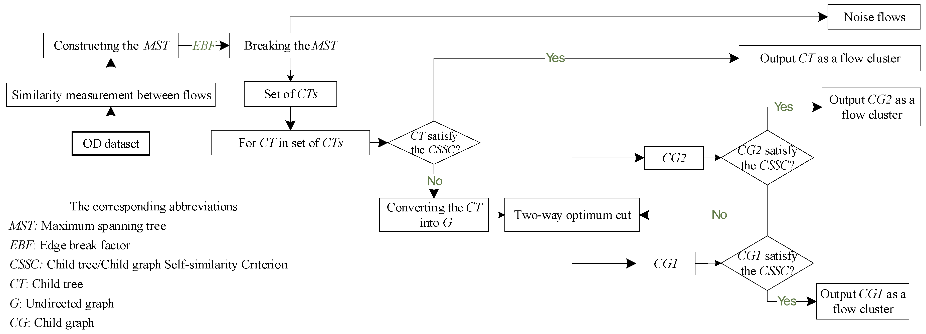
In this section, we propose a novel OD flow-clustering algorithm called “Tree-based and Optimum Cut-based Origin-Destination Flow Clustering” (TOCOFC) to obtain OD flow clusters from an enormous amount of raw OD flow data. TOCOFC can identify the spatial and spatiotemporal joint clustering of OD flow data, and different clustering results can be obtained by tuning the clustering parameters. TOCOFC has four steps. First, an OD flow similarity measurement method that quantifies the spatial similarity relationship between OD flows into a quantitative value is used. Furthermore, we extend this method to measure the spatiotemporal similarity between OD flows. Second, a maximum spanning tree MST(V, E) is constructed, and we define the similarity value between pairs of OD flows as the weight of the corresponding E. Then, we break the MST to filter the noise flows and acquire a set of child trees. Third, we develop the CSSC (Child tree/Child graph Self-Similarity Criterion) to estimate whether the OD flows (Vs) in the child tree or child graph can be organized as an OD flow cluster for output. Last, we reshape the child tree that does not satisfy CSSC into an undirected graph G(V, E). Then, a recursive, graph-based optimum-cut method is used to partition G into child graphs, and the recursion process stops when the child graph satisfies the CSSC. We repeat the partition process until all the child trees that were partitioned into child graphs satisfy the CSSC. The whole clustering process is displayed in Figure 1.

3.1. Similarity Measurement Method of the OD Flow

To ensure that there is a similarity relationship between two OD flows, it is required that these two flows are not only geographically adjacent but also remain similar in direction.

Definition 1.

Spatial similarity between OD flows: The quantitative value of the similarity relationship between two flows in terms of spatial position. The spatial similarity sim(f_i, f_j) between two OD flows f_i and f_j is defined as

$$sim\left(f_i,f_j\right)=1-func\left(ratioO\right)\ast func\left(ratioD\right)/4.$$

(1)

The variables ratioO, ratioD, and func(ratio) are defined as

$$ratioO=dist\left(O_i,O_j\right)/disLimit,$$

(2)

$$ratioD=dist\left(D_i,D_j\right)/disLimit,\mathrm{and}$$

(3)

$$func\left(ratio\right)=\{\begin{array}{cc}ratio+1& ratio\le 1\\ {\left(ratio+1\right)}^a& ratio>1\end{array},$$

(4)

where dist(O_i,O_j) and dist(D_i,D_j) represent the Euclidean distance between two origin points of a flow and two destination points of a flow, respectively. disLimit is a parameter related to the length of f_i, which we explain clearly in Remark 1, and a is a parameter used for preventing a local effect caused by the numerical value of one of the ratios (ratioO, ratioD) being extremely small, which we explain clearly in Remark 2.

The range of the similarity value of two OD flows, which are calculated by Equations (1)–(4), is 0 to 0.75. Zero is the minimum value of two similar OD flows, and the more similar the two flows are, the greater the similarity value is.

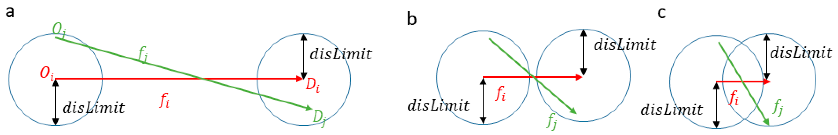
Remark 1.

In Figure 2, there are three cases used for showing the spatial similarity relationship between OD flows and proving it has to do with the length of the OD flows.

In Figure 2a, O_i and O_j are the origin points of OD flows f_i and f_j, respectively, D_i and D_j are the destination points of OD flows f_i and f_j, respectively, and the parameter disLimit is the radius of the circle whose center is O_i or D_j. If both dist(O_i,O_j) and dist(O_i,O_j) are less than disLimit, then we can say f_i and f_j are similar. However, the value of disLimit is hard to determine; if we set disLimit to a fixed value, it will cause two errors:

• Intuitively, the extent of similarity of the flows in Figure 2a is higher than that of the flows in Figure 2b, but under the circumstances of a fixed disLimit, the ratio dist(O_i,O_j)/disLimit and the ratio dist(D_i,D_j)/disLimit in Figure 2a,b are similar. That is, the quantitative error is caused by a fixed disLimit.
• In Figure 2c, f_i and f_j are obviously not similar, but they are concluded to be similar flows if they are judged by a fixed disLimit.

Thus, disLimit cannot be a fixed value. He. et al. [12] proposed that the length of an OD flow must be greater than 2disLimit/sin45° (≈2.83disLimit) to guarantee an angle between two OD flows of less than 45. Therefore, in this paper, we set disLimit to vary with the length of the flow, that is

$$disLimit=\frac{length\left(f_i\right)}{k},$$

(5)

where k is a parameter greater than 2.83. Usually, we set k to 2.83.

Remark 2.

Two ratios, ratioO (dist(O_i,O_j)/disLimit) and ratioD (dist(D_i,D_j)/disLimit), are used to calculate the similarity value of two flows to determine whether they are similar or the extent of their similarity. When both ratios are less than or equal to 1, we can say these two flows are similar, and the smaller the value of the ratios, the higher the similarity. It is worth noting that when one of the ratios is small, the similarity value calculated by the above equations is greater than 0 even when the other ratio is larger than 1, which is the local effect we mentioned above. Therefore, a piecewise function Equation (4) is proposed to prevent this local effect. In the cases where the ratio is greater than 1, the parameter a of the power function, func(ratio) in Equation (4), will alleviate this negative local effect when a is larger than 1. The larger the value of parameter a, the better the mitigation effect. One plus the ratio also achieves such a mitigation effect.

Remark 3.

Clearly, the similarity value calculated by Equations (1)–(4) has a feature: asymmetry. In other words, sim(f_i, f_j) and sim(f_j, f_i) are not equivalent when the length of f_i is not equal to the length of f_j. Although the difference between sim(f_i, f_j) and sim(f_j, f_i) is not large because there is not much difference in the length of two similar flows, we adopt the larger one as the uniform similarity value for the sake of convenience for subsequent research. With the above description, the uniform spatial similarity between two OD flows can be calculated as

$$si{m}_{f_i,f_j}=\max \left(sim\left(f_i,f_j\right),sim\left(f_j,f_i\right)\right).$$

(6)

Definition 2.

Spatiotemporal similarity between OD flows: The quantitative value of the similarity relationship between two flows taking into account the spatial and temporal information. The spatiotemporal similarity (sim_ST(f_i, f_j)) between two OD flows f_i and f_j, which is extended from Equation (1), is defined as

$$sim\_ST\left(f_i,f_j\right)=1-func\left(ratioO\right)\ast func\left(ratioD\right)\ast func\left(ratioT\right)/8,$$

(7)

where ratioT is defined as

$$ratioT=\frac{timeSpan\left(f_i,f_j\right)}{timeLimit}.$$

(8)

timeSpan(f_i, f_j) represents the time difference between OD flow f_i and f_j, and there are two ways to calculate the time difference:

• Calculating the time difference on the basis of the starting time of the OD flows.
• Calculating the time difference on the basis of the ending time of the OD flows.

If timeSpan(f_i, f_j) is larger than timeLimit, then we can say that f_i and f_j have no temporal similarity. Thus, timeLimit is a parameter similar to disLimit because both are used for calculating the ratios; however, disLimit is a parameter that depends on the length of the OD flow, and timeLimit is set artificially, without any relation to the OD flow itself. We can set timeLimit to any value, such as 5 min, 10 min, 15 min, 30 min, 45 min, and 1 h, depending on what kind of clustering results we want.

Remark 4.

The uniform spatiotemporal similarity of two OD flows is defined as follows:

$$sim\_S{T}_{f_i,f_j}=max\left(sim\_ST\left(f_i,f_j\right),sim\_ST\left(f_j,f_i\right)\right).$$

(9)

3.2. Construct the Maximum Spanning Tree and Its Child Tree

Definition 3.

Maximum spanning tree. The maximum spanning tree is a concept opposite to that of the minimum spanning tree. In an undirected connected graph, if there is a connected subgraph containing all the nodes and part of the edges of the original graph and there is no loop (or simple circuits) in the subgraph, then we call this kind of subgraph a spanning tree of the original graph. A maximum spanning tree has the maximum weight among all the spanning trees.

The variable V is a collection of OD flows, MST represents the maximum spanning tree for V, and E represents the set of edges in the MST. For each edge(u,v) ∈ E, we set the edge(u,v) weight with sim_u,_v or sim_ST_u,_v.

The MST is constructed from an arbitrary root vertex (an OD flow) and grows until the MST spans all the vertices in V. At each step in the process of growing the MST, we add the heaviest edge that connects V to an isolated vertex (one has not been added to the MST before) to the MST.

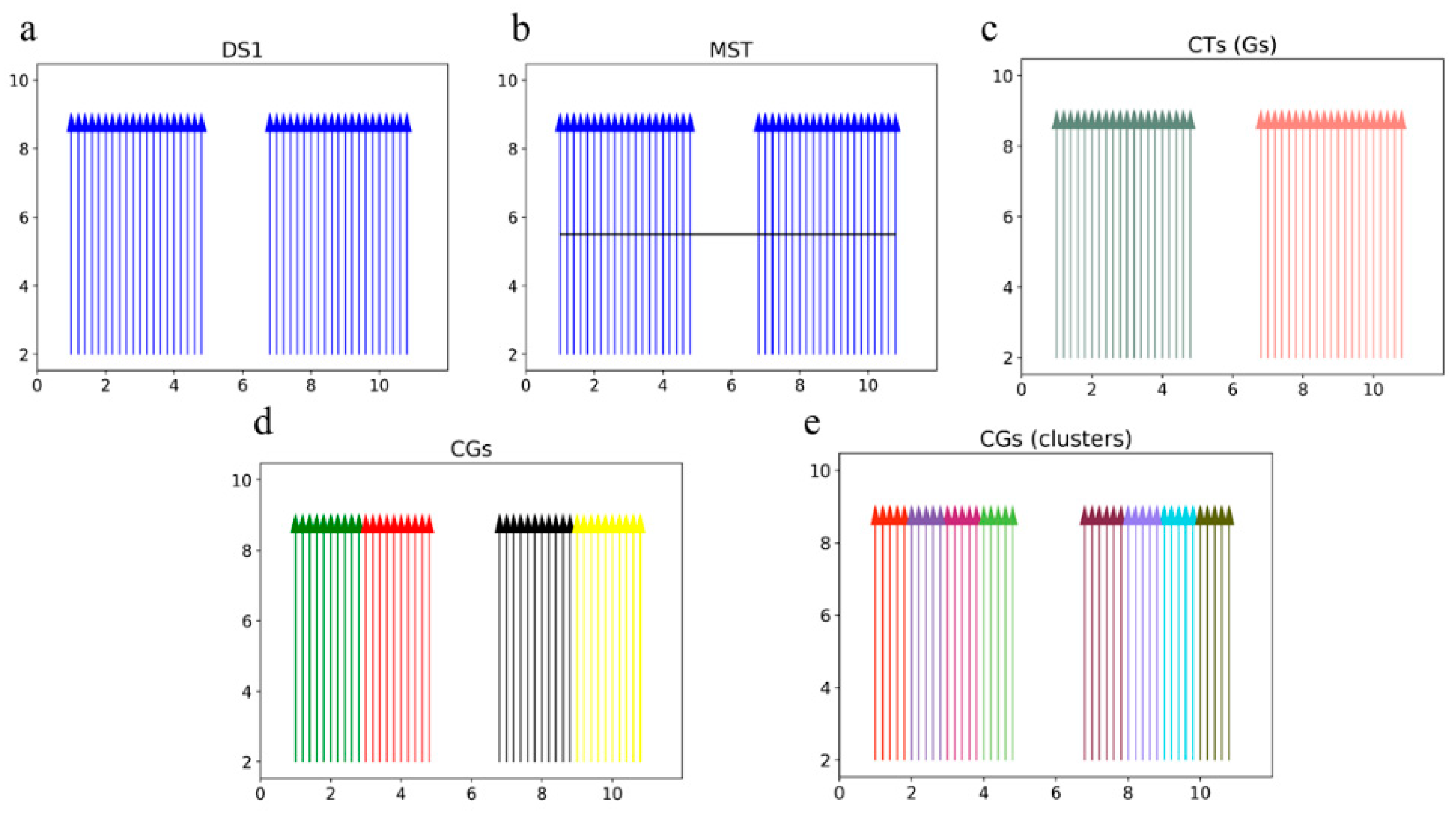
After the MST has been constructed, a factor named “Edge Breakup Factor (EBF)” is utilized to split the MST into many child trees. The value of the EBF is usually set to 0 because 0 is the lowest similarity value of two similar flows. CT denotes the child tree.

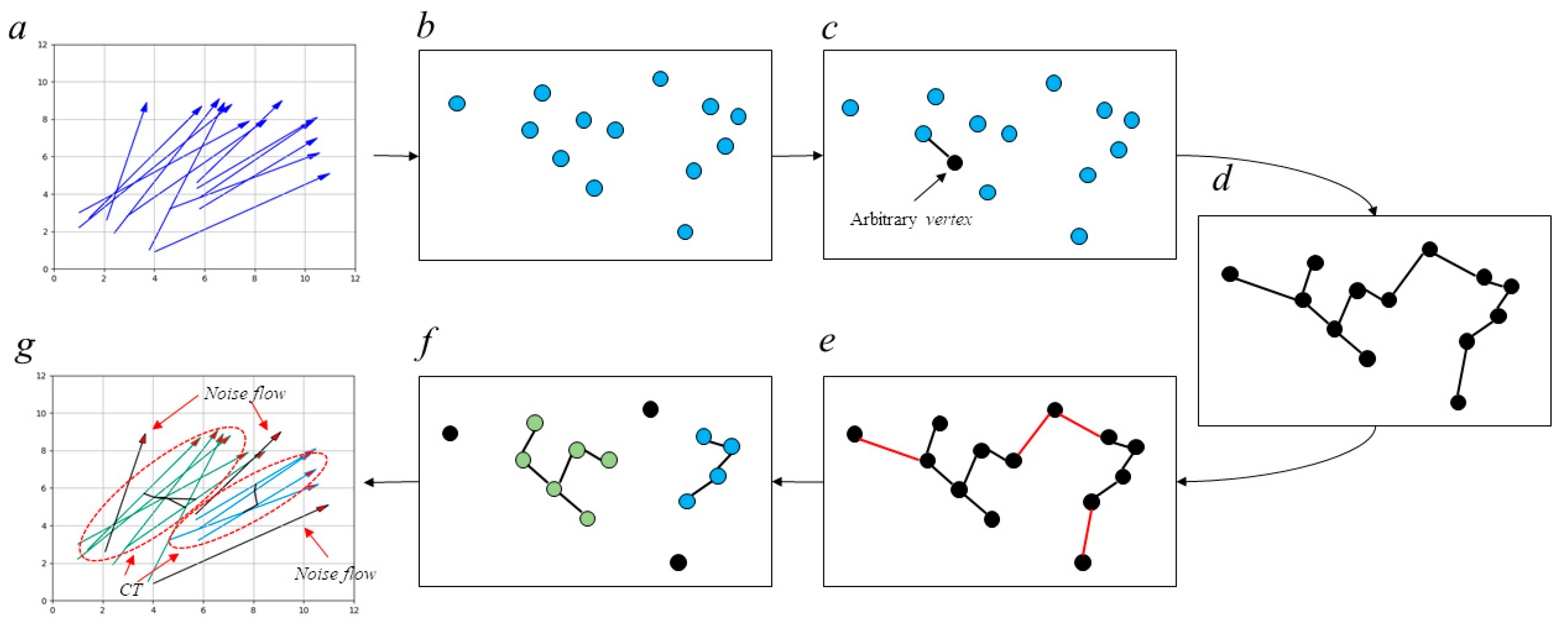
By searching for edges whose weight value is less than that of the EBF in the MST and removing them, we can obtain several relatively small CTs. A simple and intuitive example is shown in Figure 3, with the purpose of illustrating the procedure of constructing an MST and splitting it into child trees.

Remark 5.

If there exists a CT that has only one vertex and no edge, we call it a noise flow.

Remark 6.

There is no similarity relationship between the CTs. According to the characteristics of the MST, the edge with the greatest weight between the CTs is the one that has been broken up due to its weight being lower than the value of the EBF (which is actually 0), so there is no vertex (OD flow) in one of the CTs related to the other CTs.

The benefits of constructing the MST and splitting it into CTs are as follows:

• Extracting noise flows and excluding them from the next clustering steps to prevent a loss of clustering accuracy.
• Splitting the high-scale MST into several smaller CTs that do not have similar relationships to each other can increase the clustering efficiency of the subsequent steps without any accuracy loss.
• There is no similarity relationship between the CTs, so we can cluster all the CTs separately parallel to each other.

3.3. Child Tree/Child Graph Self-Similarity Criterion

Given that CTs vary widely, a criterion called Child tree/Child graph Self-Similarity Criterion (CSSC) is formulated to evaluate whether the vertices in CT can be organized as an OD flow cluster. CSSC is also applicable to the child graph, which we will introduce in the next clustering steps.

Definition 4.

Child tree/Child graph Self-Similarity. Child tree/Child graph Self-Similarity (CSS) that is used to calculate the internal similarity of CTs is defined as

$$CSS\left(CT\right)=\frac{{{\displaystyle \sum }}_{i=0}^{nu{m}_{CT}}{{\displaystyle \sum }}_{j=0,j\ne i}^{nu{m}_{CT}}si{m}_{f_i,f_j}\ge 0?1:0}{nu{m}_{CT}\ast \left(nu{m}_{CT}-1\right)/2}$$

(10)

where num_CT represents the number of vertices (OD flows) in CT, f_i represents one of the flows in CT, and so is f_j.

Definition 5.

Child tree/Child graph Self-Similarity Tolerance. The Child tree/Child graph Self-Similarity Tolerance (CSST) is an artificial threshold. For each CT, if its CCS is greater than or equal to the CCST, then we can say that all the vertices in the CT can be organized into a cluster; otherwise, the CT needs further cutting. Our method provides a simple but effective criterion for obtaining OD flow clusters, and the user can acquire their customized clustering results by modifying the CCST. However, we think it is necessary for us to give a recommended range of CCST values (CCST ≥ 0.5), which is reasonable to guarantee the sufficient similarity within the OD flow clusters.

3.4. Cut-Based Graph Clustering Method

The procedure of cut-based graph clustering is employed if there are some CTs that cannot meet the requirements of the CSSC. In this part, we first convert the CT that needs to be cut into an undirected connected graph. Then, a cut-based graph clustering algorithm using a global cut criterion is used to partition this graph into several child graphs that meet the requirements of the CSSC.

Graph theory cutting algorithm [15,22,23,24,25] is now a very mature clustering algorithm, which has very significant effects in clustering complex data.

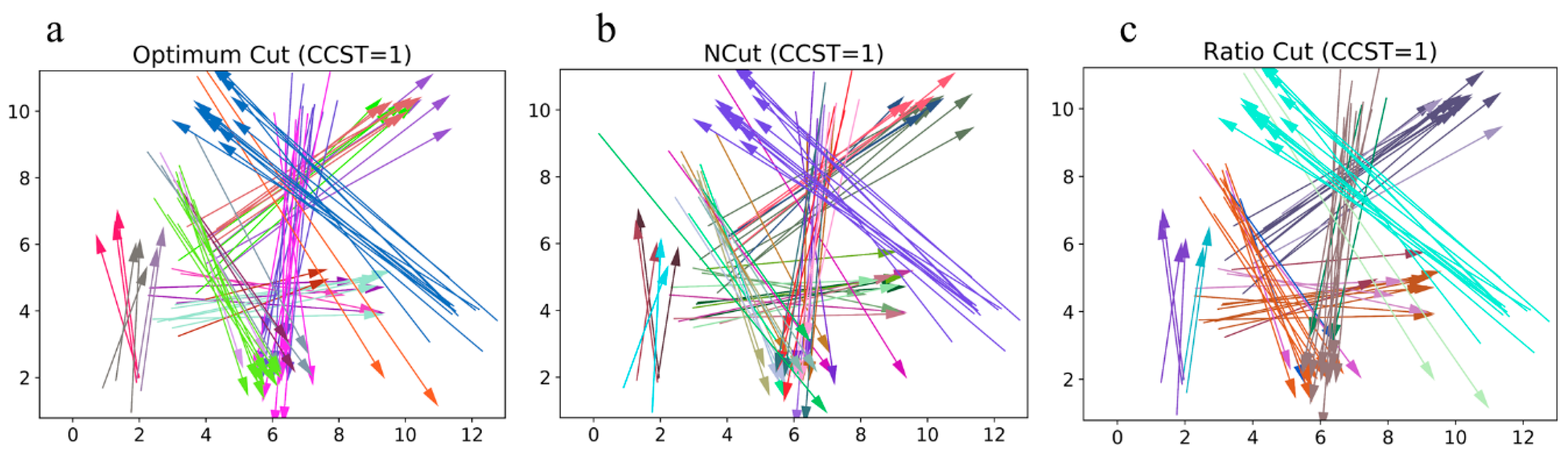
The cut-based graph clustering algorithm using a global cut criterion, also named spectral clustering, has become more popular in recent years because it is simple to implement and usually has a better clustering result than that of the tradition clustering algorithm. There have been many global cut criteria, such as the minimum cut [22], normalized cut [23] and ratio cut [26]. Although these cut criteria can indeed prevent skewed cuts efficiently, they usually perform poorly when the number of vertices in the graph is large. Considering the number of clusters required for the clustering method, based on the criteria mentioned above and the reality that CTs vary greatly, it is impossible to give an exact number of clusters to guarantee that all the clustering results satisfy the CSSC. To overcome the limitations above, a recursive two-way optimum-cut graph clustering method proposed by Li [15] is utilized to partition the graph into child graphs. We will introduce the details of this method applied in the OD flow clustering below.

Given a CT that needs to be cut, we convert it into a weighted undirected graph G (V, E) where the vertex set V is the same as the V in the CT and the edge set E is the set of unordered pairs of V. The weight of each edge is first calculated by the similarity measurement method of the OD flow, then we set the weight of the edge(u,v) with a weight less than 0 to 0. N = |V| denotes the number of vertices and W is a symmetrical matrix with W(i, j) = w(V_i, V_j), where w(V_i, V_j) represents the weight between vertex V_i and V_j.

During the clustering process, we tried to find the best cut to partition G into two disjointed child Graphs, CG1 and CG2, where CG1 ≠ Ø, CG2 ≠ Ø, CG1 ∩ CG2 = Ø, and CG1 ∪ CG2 = G.

Definition 6.

Intraweight. The intraweight (IW) of the CG is defined as

$$IW\left(CG\right)={{\displaystyle \sum }}_{i=0}^n{{\displaystyle \sum }}_{j=0,j\ne i}^{n}w\left(V_i,V_j\right).$$

(11)

Definition 7.

Cut-weight. The cut-weight (CW) of the G is defined as

$$CW\left(G\right)={{\displaystyle \sum }}_{u\in CG1,v\in CG2}w\left(u,v\right).$$

(12)

The best cut tries to minimize the value of the CW(G) and maximize the value of the IW(CG1) and IW(CG2) simultaneously. To achieve this, we propose the following optimum-cut criterion:

$$Ocut\left(CG1,CG2\right)=min(max(\frac{CW\left(G\right)}{IW\left(CG1\right)},\frac{CW\left(G\right)}{IW\left(CG2\right)})),$$

(13)

which is similar to the optimum-cut criterion proposed by Li [15].

Li [15] has discussed the feasibility of optimizing the optimum-cut criterion and gave an effective sample-based method to obtain the division results. On the theoretical basis of Li [15], the steps of the optimum cut-based graph partition are as follows:

Step 1: Given a G(V, E) converted from a CT, let d(u) = d(u) = ${{\displaystyle \sum }}_{v}w\left(u,v\right)$ be the total weight from vertex u to all the other vertices. With the definition of N and d, D is an N × N diagonal matrix with d = (d(V1), d(V2), …, d(VN)) on its diagonal. The normalized Laplacian matrix is denoted by L, which is represented as follows:

$$L=D^{-\frac{1}{2}}\left(D-W\right)D^{-\frac{1}{2}}.$$

(14)

Step 2: Let λ₂ be the second smallest eigenvalue of L, α₂ be the eigenvector corresponding to λ₂ and $x_2=D^{-1/2}{\alpha }_2$.

Step 3: Draw n (usually 400) independent random sample points uniformly from [min(x₂), max(x₂)].

Step 4: Select each sample point as a split point to partition x₂ into two parts and calculate the value of

$$max(\frac{CW\left(G\right)}{IW\left(CG1\right)},\frac{CW\left(G\right)}{IW\left(CG2\right)})$$

Step 5: Choose the sample point as the optimal split point whose value of

$$max(\frac{CW\left(G\right)}{IW\left(CG1\right)},\frac{CW\left(G\right)}{IW\left(CG2\right)})$$

is the smallest value of all the sample points. Then, use the optimal split point to bisect G into CG1 and CG2.

Remark 7.

The value of IW(CG) is 0 when the number of vertices in CG is 1, which violates the principle that the denominator must not be zero. Therefore, we replace IW(CG) with a small positive number when this situation happens.

However, this sample-based division method is not suitable for a very large amount of data because of its low computational efficiency. Thus, we chose k-means as an alternative method to partition x₂ into two parts, which was also proven to be feasible by Li [15].

Furthermore, a recursive strategy is adopted to repartition the CG that cannot meet the requirements of the CSSC. Based on the CSSC, we can decide which CT should be partitioned, which CG should be repartitioned, and when the process of recursive repartition should be stopped.

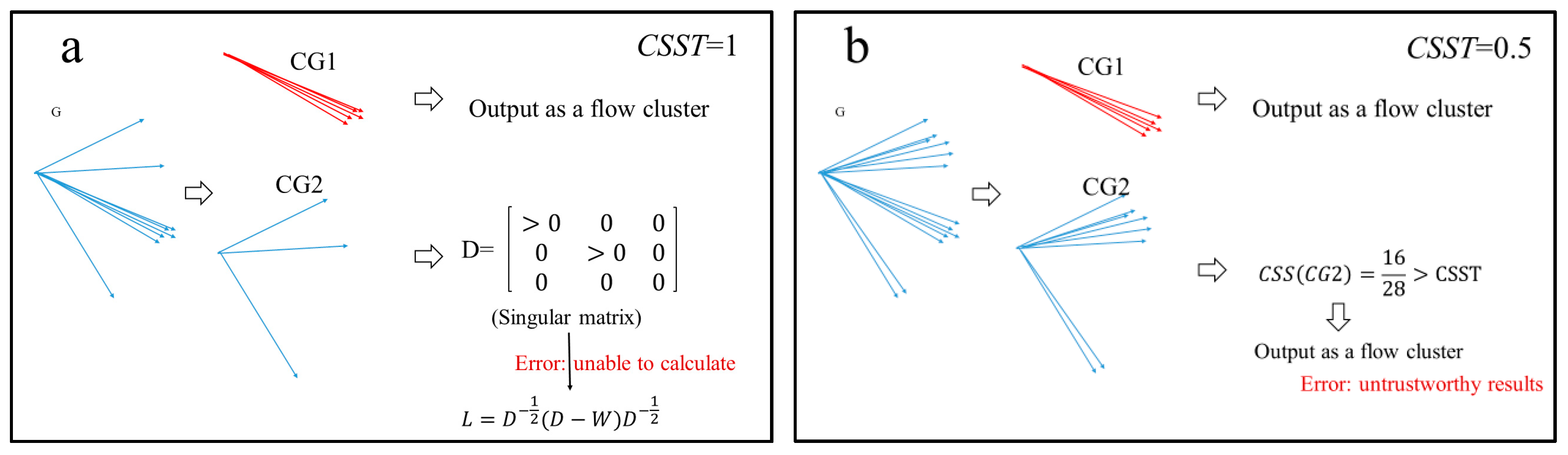
Remark 8.

Two serious problems occur in the process of repartitioning the CGs:

Problem 1.If, in the CG that needs to be further cut, there exists one or more noise flows, the matrix D corresponding to CG will be a singular matrix, which is forbidden in the process of calculating the normalized Laplacian matrix.

Problem 2.When the CSST is less than 1, there exist some CGs that satisfy the CSSC, but it can be partitioned into two CGs without any similarity relationship.

Figure 4 intuitively illustrates these two problems with two simple examples. Clearly, Problem 1 disturbs the partitioning process, and Problem 2 makes the clustering results untrustworthy.

To cope with these two problems, we extract the vertices of the CGs that exist from one of the above problems and use them to construct an MST, and then we split it into CTs; this is similar to the step that we introduced in Section 3.2, which is very helpful for dealing with these two problems.

After obtaining all the CGs that satisfy the CSSC, we organize all the vertices in each CG into a flow cluster.

3.5. Algorithm and Performance Analysis

From the description in the previous sections, it can be seen that our algorithm mainly consists of three steps:

step 1.

Compute the similarity value between flows.

step 2.

Construct the MST.

step 3.

Cut the tree or graph.

Given n OD flows, step 1 has the time complexity of O(n²) for calculating the similarity value between flows, and the result of the calculation is stored as a matrix for the subsequent steps to prevent repeated calculations. In step 2, the MST’s construction runs in time O(E+VlgV) by using Fibonacci heaps [26]. As n OD flows can be seen as n vs. and there are (n−1)*n/2 Es between the n Vs, the complexity for constructing the MST is equivalent to O(n²+nlgn). Step 3 takes O(n) to compute the diagonal matrix D in each iteration if there is no noise flow. Assuming that the MST has been split into k balanced CTs, the time complexity of computing the normalized Laplacian matrix L is O(n³/k²). It is worth noting that the weight matrix W is a sparse matrix. By using some tricks of sparse matrix operation, the time complexity of computing L can be reduced to O(n²/k²). Then, the k-means algorithm takes O(n) to partition the eigenvector. Therefore, the overall time complexity spent in the first iteration of step 3 is O(n²/k²+2n). In the worst case, the first iteration is calculated in O(n²+2n). In the next iteration, as an increasing number of flows are output as clusters, k becomes increasingly large, and the time consumption is less than that of the first iteration. Assume that the clustering process ends after m iterations, and the whole computation procedure of step 3 is less than O(m*n²+2n*m).

According to the above steps, the whole computation procedure of the TOCOFC algorithm costs approximately O((m+1)*n²+2n*m+n*lgn+n). Since m ≪ n, the time complexity of TOCOFC is approximately O(n²).

Next, we introduce the memory consumption of the TOCOFC algorithm. In step 1, the similarity value between the flows is calculated and stored as a matrix, which needs a large memory space. We realize that most of the values in this matrix are 0 because there is not a similar relationship between most flows, which means that the matrix storing the similarity information between the flows is a sparse matrix. Therefore, we use a triple table in our experiments to store useful information for practical applications, which reduces the space complexity of step 1 from O(n*n) to O(a*n) (a is the average number of similar flows). In the next steps, we use the same method to store the calculation results. The space complexity consumed by each iteration in the above iterative process is similar to or less than that of step 1. Since a ≪ n, the overall space complexity of TOCOFC is O(n).

4. Experiments and Results

In this section, we will apply TOCOFC to two artificial spatial datasets, DS1 and DS2, and two real-world spatiotemporal datasets, DS3 and DS4, to demonstrate the effectiveness of TOCOFC. To reveal the effects of the CSST and timeLimit parameters involved in TOCOFC on the clustering results, we conduct a series of related comparison experiments on these datasets.

The OD flows in the artificial spatial datasets DS1 and DS2 only include spatial information, so we use the spatial version of TOCOFC to experiment on DS1 and DS2. For DS4, we experiment with the spatiotemporal version of TOCOFC. Although DS4 includes time information, the dataset is used for comparison with previous work, so here we experiment with the spatial version of TOCOFC.

All the experiments can be separated into three groups: experiments on artificial spatial datasets, the practical application of TOCOFC and comparison with previous research.

4.1. Experiments on Artificial Spatial Datasets

Experiment 1. This experiment shows the clustering process of TOCOFC. The dataset DS1 is shown in Figure 5a, which consists of 40 OD flows of equal length. We demonstrate the clustering process of TOCOFC in Figure 5b–e. In this experiment, we set the parameter CSST to 1. As shown in Figure 5, we first built an MST and then split it into two CTs, but these CTs cannot satisfy the CSSC under CSST = 1, so these CTs are organized into Gs to be partitioned until, finally, the CGs satisfy the CSSC.

Experiment 2. In this experiment, we conduct a series of clustering steps under different values of CSST for comparison. Figure 6a shows the dataset DS2, which contains many OD flows with different lengths. The clustering results are shown in Figure 6b–g, where different clusters are depicted in different colors, and Figure 6h shows the noise flows discovered by TOCOFC when the CSST is 1. It is clear that the clusters discovered by TOCOFC become increasingly detailed as the value of the CSST increases. Apparently, in terms of identifying the intrasimilarity of the clusters, the parameters used to create Figure 6g perform better than the others. For the OD flows in the lower left corner, one cluster is discovered by TOCOFC when the CSST is equal to 0.5, and this cluster is partitioned into two clusters when the CSST is 0.6, 0.7, or 0.8. Furthermore, this cluster is split into three clusters when CSST is 0.9 or 1. However, this does not mean that the larger the value of the CSST, the better the clustering results. There still exists some strong similarity relationship between clusters that are adjacent to each other. From the clustering results, we know that the CSST is a parameter associated with the clustering results; users can choose the appropriate value of the CSST based on their demand for clustering results.

In the case of Figure 6g, there is a significant difference between the two elliptical regions in terms of the flow length, but there is not much difference in the range of OD points between these two regions. The clustering result indicates that the OD flows in the lower left ellipse are grouped into three clusters; however, the flows in the other ellipse are grouped into just one cluster. The flexible parameter disLimit, which is related to the flow length results in the abovementioned phenomenon, effectively ensures the accuracy of clustering results.

In addition, Figure 6h illustrates that TOCOFC can effectively identify noise flows that may decrease the accuracy of clustering results.

Experiment 3. To demonstrate that the optimum cut-based algorithm we used outperforms the traditional spectral clustering, such as normalized cut and ratio cut, we further use these three methods to perform a comparative experiment on DS2. The clustering results with different cutting methods are shown in Figure 7. After fully observing the details of the clustering results of these three methods, we find that our method can guarantee strong similarity within clusters, and the difference between clusters is obvious. In contrast, the normalized cut and ratio cut perform much worse in terms of the details of the clustering results. For the normalized cut, the flow in some clusters is more similar to the flow in other clusters, which means it is unable to find the genuine clusters. The ratio cut performs better than the normalized cut; however, it has the same drawback. Therefore, the optimum-cut method we adopted is the best cutting method.

4.2. Experiments on Real Datasets—A Case Study

For the purpose of illustrating the practicability of the TOCOFC algorithm, two case studies are carried out with DIDI travel datasets in this section. Our study area is Chengdu, the second largest city in western China. By the end of 2018, Chengdu had a residential population of 16.33 million in an area of 14,335 km². DIDI, founded in 2014, is one of the most popular taxi platforms in this region and has generated a large amount of data concerning residents’ travel.

The DIDI travel dataset we used, referred to as DS3 for convenience of description, has 181,172 OD flows on 1 November 2016. Unlike artificial datasets, each flow in the DS3 dataset contains position and temporal information, including the starting and ending times.

In all the remaining studies, we fix CSST to 0.7 and calculate the time difference on the basis of the starting time of the OD flow.

We first extract all the outflows of a residential area in the Huamanting community and use the spatial version of TOCOFC for these outflows to conduct an experiment to find possible problems in its practical applications. The Huamanting community is a mature high-rise residential area with complete supporting facilities. The north side of this community is the planned subcenter of the city, and the south side is the city center. There are 4446 households in the district, but the subway line does not extend to the area. Therefore, people have a relatively high demand for taxi service, so we choose Huamanting Community as a research area. In addition, the quantity of outflows is 1546.

Figure 8 illustrates all the outflows that are extracted from the DS3 dataset and the image map of the Huamanting community. The clustering results from the spatial version of TOCOFC are shown in Figure 9a, where the number of flows in each cluster exceeds 30. However, research shows a phenomenon: the value of the parameter disLimit is large when the length of the flows is long, resulting in the range of the spatial distribution of the O points or D points of the related clusters being large, which is not conducive to the accurate analysis of the taxi travel modes. As shown in Figure 9a, the spatial range of the clusters of the D points (the scope is drawn with a dashed ellipse) is very large. To guarantee that the spatial extent of the clustering results is fine enough to analyze the travel patterns of residents accurately, we give a limitation for the value of disLimit, that is, while the length of the flow exceeds 5 km, the parameter disLimit is a fixed value: 5/k km. This limitation relies on experience; users can decide whether to add this kind of limitation based on their data and their research needs. The clustering results after the above modification are shown in Figure 9b. Comparing the clustering results with the original OD flows, it is clear that TOCOFC can effectively discover flow clusters from a variety of disorganized data. Figure 9c shows the centers of the clusters, which makes the visualization easier to understand.

Further, we analyzed the impacts of the parameter timeLimit on the clustering results. In Figure 10, we demonstrate all the centerlines of the flow clusters with a flow number greater than 5 and use the average starting time of the flows in each cluster as the temporal information for that cluster. We then visualize all the flow clusters in different colors based on the temporal information for each cluster.

In Figure 10a, the time span of the flow within the cluster is approximately 30 min because the parameter timeLimit is set to 30 min. Similarly, the time span of the flow within the cluster depicted in Figure 10b is approximately one hour, etc.

Most of the outflow clusters are concentrated in the morning and at lunchtime, which are common travel times for people in residential areas. Additionally, we can identify the most popular destinations for the residents living in the Huamanting community and when they go there. Figure 11, which shows the time spans of the OD flow clusters over the area named “#1”, provides a close look at the different results caused by the timeLimit parameter. To distinguish each cluster clearly, we use different markers and colors to represent different flow clusters. The time spans of the flow clusters become longer as the value of timeLimit increases; when the value of timeLimit is 30 min, 17 flow clusters are discovered in area #1, but when timeLimit is equal to 3 h, the number of flow clusters is 3. The timeLimit parameter yields clustering characteristics that can be used for multiple different purposes: TOCOFC with a short timeLimit can be used to analyze the travel modes of the residents in a detailed way; conversely, a larger value of the timeLimit parameter will allow the analysis of the resident travel patterns from a macro perspective. In addition, the time span of the flow cluster is not strictly less than or equal to the value of timeLimit, while CSST is less than 1.

Finally, we use all the OD flows in DS3 for clustering, and the clustering parameters are set as follows: timeLimit = 3 h, CSST = 0.7, and disLimit has a limit of no more than 5/k km. The experimental results are illustrated in Figure 12. The temporal information of the flow cluster is represented by color. The quantity information of the cluster is represented by the thickness of the center flow. Among the clusters shown in Figure 12, some have an almost identical origin and destination but in different periods, which means that this kind of spatial connection of two areas exists is multitemporal. There are more inflows and outflows in the city center than in any other area. It is clear that the trips to the city center are concentrated in the morning. In the afternoon, there is a much higher probability for trips to leave from the city center than to go to the city center, which is in line with the common job-house rules. However, the DIDI taxis are only a part of the whole commuting system; for example, area 2 is the nearest subway station to area 1, so the DIDI taxi functions as a transfer system between area 1 and area 2, which is a phenomenon caused by the inadequacy of the existing public transportation system. In addition, not all the destinations for the afternoon trips or the night trips are residences; for example, area 3 is a famous nighttime attraction (the Temple of Marquis), which has many inflows at night. As seen from the simple analysis presented above, TOCOFC is an effective tool to discover spatiotemporal movement patterns.

4.3. Comparison and Discussion

The DS4 data are taken from the literature [19], so the experiment in this section mostly focuses on comparison with previous high-level research. The DS4 dataset consists of the New York City taxi trips data on a typical workday (21 January 2015), which contains the pickup and drop-off timestamps and locations of each taxi trip. We only use data from the comparison area, so DS4 does not cover all the trip data on that day. In total, there are 211,867 taxi trips.

In this experiment, we set CSST to 1. The clustering results are shown in Figure 13 and Figure 14. Figure 13 shows the spatial extents and centers of the top five flow clusters. Figure 14 shows the centers of the flow clusters in a hierarchical manner. Figure 15 shows the centers and spatial extents of the top five clusters with a maximum radius of 2.5 km, which is consistent with the experimental results of Gao [19]. Comparing Figure 13 with Figure 15, the most intuitive difference is that the results of the two methods are not exactly the same. Among the five clusters in Figure 15, the 1st, 2nd, 3rd, and 5th have an overlap between the O extents and the D extents, and the flows in the same cluster are probably moving in opposite directions. Close examination of the 5th cluster shows that the D extents of this cluster can be divided into two parts because the origin and destination positions of the cluster are close enough. Gao concentrated only on the influence of the maximum cluster radius and failed to grasp the relationship between flow similarity and the length of flow, which inevitably leads to clustering results that cannot accurately depict the movement pattern. TOCOFC, by contrast, has a much better performance, which is reflected in the flow within the same cluster satisfying the basic similarity relationship; for example, the direction of the different flows and the length of the flows is approximately the same. The similarity measurement method we proposed makes our clustering results superior to those of Gao. In addition, Gao’s method mainly aims at detecting the most significant movement pattern and neglecting the minor ones which are still important to fully understanding the travel modes of people, animals, etc. Instead, TOCOFC can discover both large volumes of flow clusters and minor flow clusters. Figure 14, which clearly shows that there are flow clusters with different volumes, demonstrates the superiority of TOCOFC. In Figure 14, the significant flow clusters show the most important patterns between origin hotspots and destination hotspots. As an effective supplement, the flow clusters with a relatively low volume show minor patterns between hotspots and nonhotspots or between nonhotspots. It is crucial for minor flow clusters to reveal the movement characteristics of nonhotspots, even if those minor flow clusters seem unimportant from a macroperspective.

Moreover, compared with previous works [12,16,19,20,21,23], TOCOFC adopts the optimum-cut strategy to maintain a balance between adjacent clusters; in other words, it makes the similarity between clusters small enough, and the intrasimilarity of each cluster large enough, rather than maximizing the volume of the clusters.

The abovementioned case studies show that our method successfully achieves the spatiotemporal clustering of flow data, which cannot be accomplished by most of the previous methods. Yao [21] proposed a spatiotemporal clustering algorithm for discovering mobility trends; however, this method adopts a stepwise strategy that separates the time information and location information during the clustering process, which inevitably damages the rationality of the clustering results. Yao’s algorithm requires there to be overlapping travel time between the flows within each flow cluster, which makes it difficult to analyze the mobility mode from multiple time scales. The TOCOFC method, by contrast, has great advantages in terms of flexibility and practicality.

In the above analysis, there is an important problem in our algorithm: the setting of parameters. This problem is mainly three-fold and includes the setting of the CSST parameter, the setting of the timeLimit parameter, and the limitation of disLimit. Regarding the CSST parameter, our suggested value varies from 0.5 to 1. If the CSST is set to 1, the internal similarity of the flow clusters is the strongest, which is reflected in all the flows remaining similar in each cluster; however, the similarity between adjacent clusters is also strong. If the CSST is set to 0.5, then the opposite situation will occur. Thus, users can choose the appropriate value of CSST according to their needs. The choice of the parameter timeLimit is also based on the user’s needs. For example, a relatively small timeLimit value can make the research on the movement pattern more precise, and a relatively large timeLimit value can drive people to grasp the time-related pattern differences from a broader time span with a more macro perspective. The limitation of disLimit also depends on the user’s needs. If the clustering results of long flow data cannot depict the movement trends accurately enough, there is a need to exert a limitation on the disLimit parameter.

The execution time of TOCOFC depends on the capacity of the dataset. Experiments on artificial datasets take no more than 10 seconds. However, TOCOFC’s computational efficiency on large-capacity datasets is lower than that in previous works. In our testing environment (i7-6700, 3.40 GHz CPU, Java), an experiment on the outflows of the Huamanting community takes nearly 3 min, an experiment on DS3 takes more than two days and an experiment on DS4 takes nearly three days. In addition, after many tests, we found that experiments on the dataset whose number of flows is greater than 250,000 will result in a memory outflow error. Low computational efficiency is the largest shortcoming of TOCOFC.

5. Conclusions and Future Work

In this paper, a novel OD flow clustering approach (referred to as TOCOFC) is presented to obtain flow clusters from raw, messy OD flows. TOCOFC develops an OD flow similarity measure to quantify the similarity relationship between OD flows. According to the selected similarity measure method, TOCOFC can be divided into the spatial version of TOCOFC and the spatiotemporal version of TOCOFC. We provide an innovative OD flow data model that regards the OD flow as the vertex of a tree (maximum spanning tree) or graph. With the target of acquiring reasonable clustering results, a recursive optimum cut-based method is used for partitioning the graph (or child graph), and a new clustering criterion, CSSC, is proposed to decide whether the tree or graph needs to be partitioned. Additionally, TOCOFC is a flexible approach from which users can acquire their customized results by setting the parameters CSST and timeLimit. Furthermore, it is easy for TOCOFC to detect noise flows that may damage the clustering accuracy.

The experiments on artificial spatial datasets confirm that the spatial version of TOCOFC can effectively identify the spatial flow clusters. A comparison of clustering results under different values of CSST indicates that TOCOFC can obtain clustering results with different precisions.

The experiments on real-world spatiotemporal datasets demonstrate that the spatiotemporal version of TOCOFC effectively extracts spatiotemporal clusters from massive real-world datasets. The parameter timeLimit can be set to different values, which is helpful for analyzing the movement patterns at different time scales.

A reasonable concern is how to evaluate the accuracy of TOCOFC. Our current evaluation method for this algorithm is mainly based on discovering the differences between the clustering results under different parameters and comparing our algorithm with others. Therefore, one of our future research directions is to develop a reasonable indicator to measure the quality of the clustering results. Another direction worth further study is the visualization of the time information of the flow clusters because the time span of the clusters obtained by spatiotemporal clustering is different.

Overall, we believe that TOCOFC can be an effective tool for the analysis of movement patterns because of its flexibility and excellent performance. In addition, TOCOFC is suitable not only for OD flows but also for interaction data that have paired location and temporal information.

References

1. Duane, M.; Gou, Z.; Lin, L. Recent Advances in the Exploratory Analysis of Interregional Flows in Space and Time. In Innovations in GIS; CRC Press: Boca Raton, FL, USA, 1997. [Google Scholar]
2. Waldo, R.T. Experiments in migration mapping by computer. Cartogr. Geogr. Inf. Sci. 1987, 14, 155–163. [Google Scholar]
3. Buchin, K.; Speckmann, B.; Verbeek, K. Flow Map Layout via Spiral Trees. IEEE Trans. Vis. Comput. Graph. 2011, 17, 2536–2544. [Google Scholar] [CrossRef] [PubMed] [Green Version]
4. Selassie, D.; Heller, B.; Heer, J. Divided Edge Bundling for Directional Network Data. IEEE Trans. Vis. Comput. Graph. 2011, 17, 2354–2363. [Google Scholar] [CrossRef] [PubMed]
5. Guo, D. Flow mapping and multivariate visualization of large spatial interaction data. IEEE Trans. Vis. Comput. Graph. 2009, 15, 1041–1048. [Google Scholar]
6. Boyandin, I.; Bertini, E.; Bak, P. Flowstrates: An Approach for Visual Exploration of Temporal Origin-Destination Data. Comput. Graph. Forum 2011, 30, 971–980. [Google Scholar] [CrossRef] [Green Version]
7. Henry, N.; Fekete, J.D. MatrixExplorer: A dual-representation system to explore social networks. IEEE Trans. Vis. Comput. Graph. 2006, 12, 677–684. [Google Scholar] [CrossRef]
8. Andrienko, G.; Andrienko, N. Spatio-temporal aggregation for visual analysis of movements. In Proceedings of the IEEE Symposium on Visual Analytics Science and Technology, Columbus, OH, USA, 19–24 October 2008; Ebert, D., Ertl, T., Eds.; IEEE: Washington, DC, USA, 2008; pp. 51–58. [Google Scholar] [Green Version]
9. Wood, J.; Dykes, J.; Slingsby, A. Visualisation of Origins, Destinations and Flows with OD Maps. Cartogr. J. 2010, 47, 117–129. [Google Scholar] [CrossRef] [Green Version]
10. Andrienko, G.; Andrienko, N. Spatial Generalization and Aggregation of Massive Movement Data. IEEE Trans. Vis. Comput. Graph. 2011, 17, 205–219. [Google Scholar] [CrossRef]
11. Wood, J.; Slingsby, A.; Dykes, J. Visualizing the dynamics of London’s bicycle hire scheme. Cartographica 2011, 46, 239–261. [Google Scholar] [CrossRef]
12. He, B.; Yan, Z.; Yu, C. A Simple Line Clustering Method for Spatial Analysis with Origin-Destination Data and Its Application to Bike-Sharing Movement Data. ISPRS Int. Geo Inf. 2018, 7, 203. [Google Scholar] [CrossRef]
13. Zhong, C.; Miao, D.; Pasi, F. Minimum spanning tree based split-and-merge: A hierarchical clustering method. Inf. Sci. 2011, 181, 3397–3410. [Google Scholar] [CrossRef]
14. Jothi, R.; Mohanty, S.K.; Ojha, A. Fast approximate minimum spanning tree based clustering algorithm. Neurocomputing 2018, 272, 542–557. [Google Scholar] [CrossRef]
15. Li, X.; Zheng, T. Optimum cut-based clustering. Signal Process. 2007, 87, 2491–2502. [Google Scholar] [CrossRef]
16. Guo, D.; Zhu, X. Origin-Destination Flow Data Smoothing and Mapping. IEEE Trans. Vis. Comput. Graph. 2014, 20, 2043–2052. [Google Scholar] [CrossRef] [PubMed]
17. Zhu, X.; Guo, D. Mapping Large Spatial Flow Data with Hierarchical Clustering. Trans. GIS 2014, 18, 421–435. [Google Scholar] [CrossRef]
18. Zhu, D.; Huang, Z.; Shi, L.; Wu, L.; Liu, Y. Inferring spatial interaction patterns from sequential snapshots of spatial distributions. Int. J. Geogr. Inf. Sci. 2018, 32, 783–805. [Google Scholar] [CrossRef]
19. Gao, Y.; Li, T.; Wang, S.; Myeong-Hun, J.; Kiumars, S. A multidimensional spatial scan statistics approach to movement pattern comparsion. Int. J. Geogr. Inf. Sci. 2018, 32, 1304–1325. [Google Scholar] [CrossRef]
20. Ci, S.; Tao, P.; Ting, M.; Yunyan, D. Detecting arbitrarily shaped clusters in origin-destination flows using ant colony optimization. Int. J. Geogr. Inf. Sci. 2019, 33, 134–154. [Google Scholar]
21. Yao, X.; Zhu, D.; Gao, Y. A Stepwise Spatio-Temporal Flow Clustering Method for Discovering Mobility Trends. IEEE Access 2018, 6, 44666–44675. [Google Scholar] [CrossRef]
22. Mishra, G.; Mohanty, S.K. A fast hybrid clustering technique based on local nearest neighbor using minimum spanning tree. Expert Syst. Appl. 2019, 132, 28–43. [Google Scholar] [CrossRef]
23. Shi, J.; Malik, J. Normalized cuts and image segmentation. IEEE Trans. Pattern Anal. 2000, 22, 888–905. [Google Scholar]
24. Hagen, L.; Kahng, A.B. New spectral methods for ratio cut partitioning and clustering. IEEE Trans. Comput. Aided Des. 1992, 11, 1074–1085. [Google Scholar] [CrossRef]
25. Lingaya, S.R.; Gerardo, B.D.; Medina, R.P. Modified Graph-theoretic Clustering Algorithm for Mining International Linkages of Philippine Higher Education Institutions. IJACSA 2019, 10, 90–95. [Google Scholar] [CrossRef]
26. Thomas, H.; Charles, E.; Ronald, L.; Clifford, S. Graph Algorithms. Introduction to Algorithms, 3rd ed.; The MIT Press: Cambridge, MA, USA, 2009; Volume 1, p. 624. [Google Scholar]
Figure 1. The whole process of Tree-based and Optimum Cut-based Origin-Destination Flow Clustering (TOCOFC).
Ijgi 08 00477 g001
Figure 2. Similarity relationships with same disLimit values and different OD flow lengths: (a) Flows with long lengths; (b) Flows with middle lengths; (c) Flows with short lengths.
Ijgi 08 00477 g002
Figure 3. Schematic illustration of the method for constructing a maximum spanning tree (MST) and its child trees (CTs): (a) The original OD flows; (b) Treating the OD flows as vertices; (c) Constructing the MST starts with an arbitrary vertex and finding the heaviest edge that connects the MST and an isolated vertex step by step; (d) the MST; (e) Finding the inappropriate edges; (f) Removing the inappropriate edges; (g) the CTs and noise flows.
Ijgi 08 00477 g003
Figure 4. Illustration of the two problems ((a) Problem 1 and (b) Problem 2).
Ijgi 08 00477 g004
Figure 5. Illustration of the clustering process. (a) DS1; (b) MST (maximum spanning tree); (c) CTs (child trees); (d) CGs (child graphs) obtained by partitioning the Gs; (e) CGs obtained by partitioning the CGs.
Ijgi 08 00477 g005
Figure 6. Clusters discovered by TOCOFC under different values of the Child tree/Child graph Self-Similarity Tolerance (CCST): (a) Raw data se tDS2; (bg) Different clustering results when the parameter CCST is equal to 0.5, 0.6, 0.7, 0.8, 0.9, 1.0; (h) Noise flow detected by TOCOFC when the parameter CCST is equal to 1.
Ijgi 08 00477 g006
Figure 7. Clusters discovered by different spectral clustering methods: (a) Clusters discovered by optimum cut; (b) Clusters discovered by NCut; (c) Clusters discovered by Ratio cut.
Ijgi 08 00477 g007
Figure 8. Illustration of the outflows of the community of Huamanting.
Ijgi 08 00477 g008
Figure 9. Clustering results by the spatial version of TOCOFC: (a) Clusters; (b) Clusters (the parameter disLimit has a limitation); (c) Centers of the OD flow clusters.
Ijgi 08 00477 g009
Figure 10. Clustering results produced by the spatiotemporal version of TOCOFC with different timeLimit values. (a) Parameter timeLimit is equal to 30 min; (b) Parameter timeLimit is equal to 1 h; (c) Parameter timeLimit is equal to 1 h and 30 min; (d) Parameter timeLimit is equal to 2 h; (e) Parameter timeLimit is equal to 2 h and 30 min; (f) Parameter timeLimit is equal to 3 h.
Ijgi 08 00477 g010
Figure 11. Time spans of the flow clusters under different values of timeLimit.
Ijgi 08 00477 g011
Figure 12. Clustering results for those OD flows whose number is greater than 40.
Ijgi 08 00477 g012
Figure 13. Top five flow clusters discovered by TOCOFC.
Ijgi 08 00477 g013
Figure 14. Centers of the flow clusters with different volumes.
Ijgi 08 00477 g014
Figure 15. Top five flow clusters discovered by Gao’s method.
Ijgi 08 00477 g015