Performance Testing of istSOS under High Load Scenarios

Abstract

In the last 20 years, a mainstream in Earth information and decision making has been drawn by the vision of the digital earth that calls for 3D representation, interoperability and modelling. In this context, the time dimension is essential but despite its importance, not many open standards and implementations are available. The Sensor Observation Service from the Open Geospatial Consortium is one of them and was specifically designed to collect, store and share timeseries of observations from sensors. To better understand the performance and limitation of one software implementation of this standard in real cases, this study executed a load testing of the istSOS application under a high load condition, characterized by a high number of concurrent users, in three cases mimicking existing monitoring networks. The results, in addition to providing reference values for future similar tests, show the general capacity of istSOS in meeting the INSPIRE quality of service requirements and in offering good performance with less than 500 concurrent users. When the number of concurrent users increases to 1000 and 2000, only 80% of the response times are below 30 seconds, performance that is unsatisfactory in most modern usages.

1. Introduction

Along with the evolution of digital technologies in recent years, we have seen the rise of the Open Science concept that emphasizes the need of different declinations of openness to optimize the benefits of investments in research. Open education, open software, open standards, open data, and open access are only some of the approaches that foster the sharing, reusing and application of scientific works, which in turn aims at providing high quality and fair access to knowledge. This paper focuses on the performance analysis of an open geospatial software that implements an open geospatial standard used to collect and share monitoring data: this permits a better understanding of the current capability and limitations of this solution in meeting the needs posed by the current state of the art.

1.1. Earth Information and Decision Making

In the last 20 years, a mainstream in Earth information and decision-making has been drawn by the vision of the digital earth proposed by Gore in 1998 [1]. Since then, many steps have been taken toward the idea of a virtual environment, where the user can explore time and space dimensions, going from coarse to granular through a multitude of layers of information, to better understand and take optimal decision. A decade later, Goodchild [2] identified the challenges that were still to be addressed: (i) visualization and ease of use, (ii) interoperability and mashups, and (iii) modelling and simulation.

In the last decade, the visualization and the ease of use requirements are largely met thanks to the availability of the so-called virtual globes [3]. Pioneered by Google Earth [4] and NASA Word Wind [5] currently Virtual Globes are widely available from different vendors, for example ESRI (ArcGIS Explorer) or open source projects like Cesium [6], and often take advantages of the latest technologies like WebGL that permit their integration in Web browsers. An interesting review of the existing solution has been presented by Keyers [7]. Recently, many efforts were directed toward the integration of these globes with civil data integrating GIS and BIM [8] to permit an incredible level of detail in data representation and exploration.

Similarly, to visualization, interoperability and mashups requirements have been addressed in the latest 10 years by a number of initiative and projects worldwide; some examples are: INSPIRE [9], GEOSS [10], enviroGRIDS [11], ACQWA [12], and GMES [13]. At the same time, a number of Open Standards from the Open Geospatial Consortium (OGC) have been defined and become a de-facto standard for the Web based geospatial technologies [14]. OGC standards enabled the interoperable delivery of maps via Web Mapping Services (WMS), the distribution of geospatial vectors and raster layers respectively through the Web Feature Service (WFS) and the Web Coverage Service (WCS). Standardized accessibility to data processing can be achieved by means of Web Processing Services (WPS). Data from sensors can be standardized by using the Sensor Observation Service (SOS) [15,16] or the SensorThings API [17], which define the interface for collecting and dispatching information on systems and observations. Standard metadata are defined by the International Organization for Standard (ISO): 19139 (metadata encoding), 19115 (resource metadata), and 19119 (service metadata) and are made accessible for search by the Catalog Service for the Web (CSW). Today, some of these standards are widely adopted and/or officially endorsed (e.g., by the INSPIRE directive) while others have not yet been extensively diffused.

Modelling and simulation have also evolved dramatically in recent years by following the growth in computing power and data availability. If we look at hydrological modelling for example, we are facing a growing interest toward hyper-resolution global models [18], which run at incredibly high resolutions in time (from 1 day to few hours and less) and in space (from 0.1 to 1 km). This evolution of models today requires the meeting of several challenges, including: (i) the need for optimization of processing costs which exponentially increase with the resolution and (ii) the necessity to obtain and process updated input data and (iii) the desire to validate the simulation results.

It is clear that georeferenced data have a central role in this digital Earth vision, thanks to their ability to be correctly visualized in space, to be spatially mashed-up and integrated, and to support accurate modelling. The ability to understand the environment in which we live and its evolution in time, which is a key factor for the sustainable management of environmental resources and the development of a safe society, depends on the timeliness, quality, completeness, and availability of these data [19,20,21,22,23].

1.2. Spatio-Temporal Observaions and Sensor Observation Services

In line with the objectives of the digital Earth, GIS science today includes the handling of spatio-temporal dimensions [24]. Specifically, as discussed by Gong et al. [25], there is the need for both temporal GIS (T-GIS) and real-time GIS (RT-GIS), which differs depending on the emphasis given in the final scope: recording and accessing historical data (time-series) or live current data (data stream). It is clear that while the main challenge of T-GIS is big data, the focus of RT-GIS is more on time efficiency. Nevertheless, both these requirements are important aspects in both scopes.

Thanks to the implementation of several services like the Open Data Cube [26] and the Google Earth Engine [27] satellite images, which are available from a number of freely and openly accessible repositories, are today increasingly used for addressing a large number of environmental analysis. Conversely, the lack of collaboration and standardization in sharing in-situ data has often prevented the conduction of data processing over larger geographic domain; as a consequence, the attention to in situ monitoring has declined [28]. However, there is an individuated scientific need of supporting ground-based measurements that are capable to make observations at typically higher spatial and temporal resolution which are essential for validation and calibration of satellite data and for measuring phenomena poorly suited to remote measurement [29] like for example the groundwater level or the underwater Phycocyanin concentration.

A possible response to the needs of data from in-situ sensor, is given by the protocols defined by the Sensor Web Enablement (SWE), which have been successfully used in several projects and applications [30] ranging, for example, from NASA’s Earth Observation [31] to German–Indonesian Tsunami Early Warning System [32], environmentally optimized irrigation systems [33] or integrated in situ ocean monitoring [23]. Those successful implementations, and many others, demonstrated that the usage of these standards may pave the way for enabling the required data interoperability and reusability in different applications.

Nevertheless, at the time of writing, the diffusion of the OGC-SWE protocols is not as large as desirable to make of it the de facto standard for sensor network spatio-temporal data. Possible reasons supposed by the authors of this paper are: (i) the commonly adopted market strategy of sensor vendors to bind customers by providing closed solution for data access; (ii) higher payload and verbosity of the SOS compared to proprietary solutions, which are often not semantically annotated; (iii) lack of open solutions that offer simple-to-use and demonstrated robustness in production environments.

1.3. Motivation of Research and Outline

Despite some SOS implementation being available on the market, at the current knowledge of the authors, no studies on performance of any SOS software are available in the literature to evaluate their applicability in real cases. Poorazizi et al. [34] evaluated the performance of three SOS software implementations in serving data under varying number of sensors and filters on area and time interval but only under normal condition (a single user). The performance evaluation of SOS implementations under high loads (concurrent users) and varying data serving scenarios mimicking existing environmental monitoring network is currently not available in literature.

To partially fill this gap, this study presents a performance evaluation of a specific SOS implementation. While we recognize the importance in evaluating and comparing different existing SOS solutions like for example 52°North SOS [35] and Mapserver [36], this study is focalized on the istSOS project only. We believe the results of this study can highlight general issues in serving spatio-temporal observations and pinpoint reference values for future comparison with other SOS software or similar standard implementation (e.g., SensorThingsAPI). Additionally, as discussed by Zhu [37], the results of a performance testing permit developers to identify strengths and weakness of a system and consequently to improve the service capability to meet user requirements, so this evaluation will support the istSOS community in software improvement. In the next section, a brief introduction of the istSOS project is described.

1.4. istSOS

In 2010, during a renewal of the hydro-meteorological monitoring network of the Canton Ti-cino, the Institute of Earth Sciences at the University of Applied Science and Arts of Southern Switzerland (IST-SUPSI) started the development of an implementation of the Sensor Observation Service standard from the OGC named istSOS [38]. As described in detail in Cannata et al. [39] the software has been based on the objective of creating a simple and open source implementation of the Sensor Observation Service standard written in Python language. This standard met the needs of collecting observations in near-real-time from the sensors, publishing information on the monitoring system and sharing data in near-real-time in an interoperable way.

From the beginning, the istSOS software has tried to incorporate IST-SUPSI’s 20 years of expertise in hydro-meteorological monitoring network management into the application. In 2010, Cannata and Antonovic identified a number of open issues of the SOS version 1.0.0 and for this reason, istSOS started to implement a number of “special features” with the aim of extending the standard capabilities and meet the more practical requirements derived by best practices and guidelines. As a result, today, istSOS has a Web based administration interface (see Figure 1) that permits access to all the service configurations and operations without need of explicitly writing XML requests, making the usage of SOS more user-friendly. In particular, using the Web interface, it is possible to create a new instance and configure it by: setting the database connection; defining the service provider and identification metadata; specifying the coordinate system used for data storage and those accepted for reprojection. It is also possible to define the maximum data-period length accepted with a single request; to create and organize the offerings (groups of sensors); to register new sensors to the network; and define virtual procedures as on-the-fly data processes. Finally, the administrator can define dictionaries of accepted observed properties, units of measures and data quality levels. From the same interface, it is possible to access the data management section that permits to manipulate the data by applying a time-series-calculator or manually adjust the values and the data quality indexes. A data viewer interface is available seamlessly to explore the data in space and time, analysing the different observed properties and plotting for the selected period one or two properties from more sensors.

From a technical point of view, istSOS follows the Web Server Gateway Interface (WSGI) specification [40], so that it can be run on any WSGI compliant web server and offers, in addition to the standard SOS service based on XML, a RESTful interface based on the JSON format.

Some of the remarkable “special features” currently supported by istSOS are:

• server-side data aggregation based on basic statistics (mean, sum, count, max, min);
• time-space re-projection of data based on user-specified coordinate system and time zone;
• observation quality management and assessment through automatic data quality checks on insertion;
• on the fly data processing with virtual procedures offered as a regular sensor (e.g.,: serving reference evapotranspiration by observing temperature, relative humidity, wind velocity, and solar radiation);
• multiple data output formats like CSV, JSON and O&M;
• restful Web API for service configuration and data elaboration through JSON format;
• notification service to monitor and dispatch messages when specific conditions are met;
• security, authentication & authorization system based on user’s role: admin, network manager, data manager and viewer.

istSOS has been used in several research applications in recent years [37,39,41,42,43] and is currently undergoing the incubation process of OSGeo, which is aiming to promote the highest quality Open Source Geospatial Software. This process is exploited by verifying that the project has a successfully operating open and collaborative development community, has clear Intellectual Property (IP) oversight of the code and implements OSGeo operating principles of having: (i) clear documentation on how it is managed, (ii) maintained developer and user documentation, (iii) maintained source code management system, (iv) maintained issue tracking system, (v) maintained project mailing lists, (vi) automated build and smoke test systems. istSOS successfully passed OGC compliance tests for SOS version 1.0.0 and 2.0.0.

2. Materials and Methods

2.1. Testing Approach

The performance testing in this study is conducted using the load testing approach. Load testing is a particular procedure aimed at measuring the response of a service when put under stress; this is to measure the service behaviour and performance under normal and peak load conditions. As defined by Menascé [44], the test is done using software that simulates the service usage in terms of users’ (not only humans) behaviour and number. The user behaviour is detailed specifying what requests are executed and with what frequency, while the user number is simulated by specifying the number of concurrent users. The results of load testing are metrics that identify the system resource statistics of the server and the performance of the service.

For the scope of this research, among the numerous tools available for conducting load testing, the authors selected the open source framework named Locust [45]. The selection was due to: its open license, its Python language, which perfectly fit with istSOS, and its event-based (not thread-bound) architecture, which make it possible to benchmarking thousands of users from a single machine. Locust is a scalable and distributed framework developed in Python and available under the MIT-license. This framework enables the set-up of a load test under different scenarios, identified by the number of concurrent users and the hatch-ratio, which indicates the users spawned for seconds. Without entering in technical details of the tools functionality, which can be found in Cannata et al. [46], it is possible to simulate the users’ behaviours by coding different user types each characterized by its relative access frequency, the set of operations they are executing, and the minimum and maximum waiting time between requests.

In each set of operations, it is possible to implement the task to be performed (generally a HTTP requests), to associate a relative execution frequency of the operation and to catch responses that are considered an operation failure (e.g., a returned error message with HTTP status code 200). Creating and combining the collection of operations and user types, it is possible to define the test in code, a fact that provides a high degree of freedom and that facilitates the definition of realistic load tests that actually simulates the desired user behaviour.

Locust allows collecting information on: number of executed requests, number of failed requests, average content size and number of requests per second, response time statistics (i.e., min, max, ave, median). During the load testing, the dstat tool [47] was used to record hardware statistics of the server. This tool allows the monitoring of all the system resources instantly and the direct writing of date, time and metrics to a comma separated values file. The combination of user and server statistics permits to evaluate the whole system performance and behaviour.

2.2. Testing Environment (System Configuration)

In order to perform the tests, two different machines where used: a physical server with the application under test and a physical client which generates the load. Virtual environments were appropriately excluded to prevent possible interferences and I/O latencies due to the virtualisation layer. The configurations of the two used machines are described in

Table 1. Hardware configuration for the load testing experiments.

	Server Configuration	Client Configuration
HD	1TB SSD (I/O 520 MB/s)	500GB HDD (I/O 520 MB/s)
CPU	i7-5820K (6 cores / 12 threads)	i7-3770 (4 cores / 8 threads)
RAM	32GB	8GB
OS	Linux Ubuntu 14.04	Linux Ubuntu 14.04

.

On the client side, a Locust environment has been installed and each test has been implemented to record the average number of requests and the response time for each request type for each minute. On the server side, the dstat tool was configured to record the usage of processors (CPU), the usage of the memory (RAM) and the disk performance (I/O—write and read speed) for each minute. The tests were conducted on the istSOS version 2.3. It can be reasonably assumed that during the tests, the measured response time is not affected by any data jam at the production stream since the 1 GB/sec transport rate of the used network is certainly faster than the service response.

2.3. Experiment Definition and Set-Up

Using the previously described selected technologies and configurations, this research tested three different monitoring networks inspired by real case applications. The tested monitoring systems are different in terms of number of sensors, length of stored time series, number of observed properties per sensor and measurement frequency.

The first real case mimics a regional monitoring system: the OASI air-quality monitoring network from the Canton Ticino [48] where about 20 stations measure three observed properties (PM10, O3 and NO2) every 10 minutes. Data are available for the last 25 years. This monitoring network can be considered as mid-size monitoring network with regard to the number of sensors and the number of archived observations (about 100 million).

The second case replicates a national monitoring system: the SwissMetNet (Landl et al., 2009). It is the automatic monitoring network of the MeteoSwiss that comprises 160 stations measuring seven meteorological parameters (air temperature, precipitation, relative humidity, hours of sunshine, wind speed, global radiation, air pressure) with a resolution of 10 minutes. Digital data are available with this time resolution from the 80s. This monitoring network can be considered of large-size in terms of number of stations and number of measurements (about 1700 million).

The third mimicked case is another regional monitoring system: the Canton Ticino GESPOS monitoring network. It collects the regional springs, wells and bore-hole observations. It counts 5120 sensors that register often a single property (e.g., groundwater head, spring flow or water temperature) measured a few times only. Data are therefore sparse in time but the observed interval is about 45 years, ranging from the 70s to the current days. This monitoring network can be considered large-size because of the number of sensors. The tested synthetic monitoring systems, inspired from the three described real case monitoring networks, has been configured as described in

Table 2. Configuration of the tested monitoring systems inspired by real case applications.

Monitoring System A—Inspired by OASI Air-Quality
N. sensors	20
Observed interval	25 years
Observed properties per sensor	4
Measurement frequency	10 minutes
Monitoring System B—Inspired by SwissMetNet Weather
N. sensors	130
Observed interval	25 years
Observed properties per sensor	10
Measurement frequency	10 minutes
Monitoring System C—Inspired by GESPOS Springs & Wells
N. sensors	5100
Observed interval	2 years
Observed properties per sensor	1
Measurement frequency	1 month

, and the database has been filled with synthetic data.

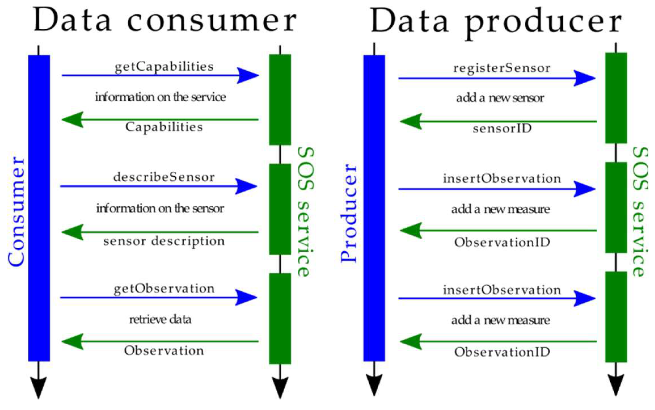
During the tests, two different types of user has been configured in Locust. One reflecting a data consumer and one reflecting a data producer (see Figure 2). The data producer is likely a sensor that registers once to the system (SOS’s registerSensor request) and then starts to send observations at its sampling frequency (SOS’s insertObservation requests). The data consumer is likely a human that looks at the service capabilities (SOS’s getCapabilities request), then individuates the sensor of its interest, looks for its specifications (SOS’s sensorDescribe request) and finally download the data (SOS’s getObservation request).

Each monitoring system of Table 2 has been tested under different scenarios with increasing number of concurrent data consumers: 100, 200, 500, 1000, and 2000. Data producers are equal to the number of sensors of the tested monitoring system. In order to assign different relative frequencies to the different SOS requests performed by data consumers, weights derived from previous experiments have been used. In particular, the weights values were derived from the results presented in Cannata and Antonovic [33], where the total number of executed SOS requests for each type over a period of two years were extracted from the analysis of server logs of an istSOS service used in the ENORASIS projects. As a result, the selected relative weights of the requests applied during the tests are reported in

Table 3. Relative weights of Sensor Observation Service (SOS) requests used for the data consumer user type during the test’s execution.

SOS Requests	Weight
getCapabilities	1
describeSensor	5
getObservations	100

.

While getCapabilities and describeSensor do not have complex filter capabilities, the getObservation request allows the selection of a period in time and the observed properties. During the execution of the tests, we decided to retrieve all the observed properties along a time interval randomly shifted in time within the data observed period. The time interval has been selected as a fixed period that is proportional to the observation frequency. For the system A and B the period was set to 1 day and for case C to 6 months. During the testing, data producers and data consumer operated simultaneously using the same SOS service.

In addition to the different scenarios tested for the different monitoring systems (A, B and C), the tests were conducted on two different WSGI server applications:

• gevent
• mod_wsgi

mod_wsgi [49] is the Apache module to run Python application service and it is the environment where istSOS has been tested and therefore is the suggested server by the istSOS community. gevent [50] is a coroutine-based networking library that was selected as an alternative due to its promising results. In fact, in Piël [51] a benchmark test comparing several WSGI server application showed that gevent has low server latencies, system loads, CPU usage, response times and error rates.

While gevent configuration was limited to set the number of processes to 12, mod_wsgi has been configured with the following Apache MPM (Multi-Processing Module) worker module settings: StartServers = 12; MinSpareThreads = 50; MaxSpareThreads = 300; ThreadLimit = 128; ThreadsPerChild = 100; MaxRequestWorkers = 300; MaxConnectionsPerChild = 0. Interested readers can find details of theese parameters in the official Apache MPM worker documentation [52].

Response sizes vary per different scenarios while requests sizes are constant within a single test since the number of sensors and data inserted and requested are fixed within the test execution. Values are listed in

Table 4. Size of requests and responses in KB for different tasting case and SOS request.

	Case A		Case B		Case C
	Request (KB)	Response (KB)	Request (KB)	Response (KB)	Request (KB)	Response (KB)
GC	0.685	21.3	0.685	77.2	0.685	2500
DS	0.541	4.4	0.541	6.1	0.539	3.2
IO	3.9	0.215	5.800	0.216	-	-
GO	0.925	58.4	0.925	102.2	0.923	4.6

.

2.4. Reference for the Evaluation of the Results

To analyse the performance of a service, which is an important aspect of the so-called Quality of Service (QoS), several metrics were used in literature [53,54,55] but two of them are particularly prominent: the availability and the response time. While the availability indicates if a user has access to a web resource, the response time shows how fast this happens. During the load testing these two aspects help to assess how well a user will be satisfied with the web service.

To quantitatively evaluate the results of the tests there is the need to identify a reference. To this end, we selected as reference the Quality of Services (QoS) defined by INSPIRE in the requirements for network services. The QoS for INSPIRE is defined in the implementing directive 2007/2/EC (regulation (EC) No 976/2009) which specifies three criteria: performance, capacity and availability. While the service performance should guarantee to continuously serve the data within given time limits, capacity must handle at least a defined number of simultaneous users without degrading the performance, and availability must guarantee 99% of uptime, excluding planned breaks due to service maintenance. Specific values of limits and concurrent users for performance and capacity are defined in appropriate technical guidance documents for different service type; for example: discovery service like CSW, view service like WMS or download service like WFS. Currently, it seems that there’s no Technical Guidance (TG) on quality of service for SOS, nevertheless in the “Technical Guidance for implementing download services using the OGC Sensor Observation Service and ISO 19143 Filter Encoding”, it is stated that specification of TG for WFS can serve as an orientation for implementing QoS for SOS. TG for download services sets the performance limit to 10 seconds to receive the initial response in normal situation to retrieve metadata (e.g., describe spatial data set) and 30 seconds to retrieve data (e.g., get spatial data set). After that, the downstream speed must be higher than 0.5 MB/s. The capacity criterion is that 10 requests per second are served within the performance limits.

3. Results

The presented results of the load testing are related only to the requests that are repeated in time (therefore excluding the registerSensor request executed only once per sensor at database initialisation). Herein after, we will refer to the different SOS requests with the following acronyms:

• IO for insertObservation,
• RS for registerSensor,
• GO for getObservatin,
• DS for describeSensor,
• GC for getCapabilities.

Test results related to a specific request and number of concurrent users will be referred with the acronym of the request followed by the number of concurrent data consumers (e.g., GC500 for the test of getCapabilities request with 500 concurrent users). Finally, specific tests conducted with a selected WSGI interface will be designated with the suffix “m” for mod_wsgi and “g” for gevent, so DS200m refers to results of describeSensor request with 200 concurrent data consumers using the mod_wsgi server application.

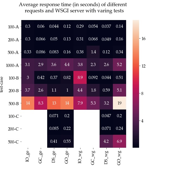
3.1. Case A: Air-Quality Monitoring Network in Ticino

Average response time for different SOS requests are illustrated in Figure 3 in logarithmic scale.

Table 5. Requests per second (total and for different SOS request) with different concurrent data consumers and WSGI applications for the test case of a medium size monitoring network (case A). Rate of failure (ρ) is reported when errors have been detected.

Request	IO	GC	DS	GO	TOT
100m	0.03	0.10	0.47	7.45	8.06
200m	0.03	0.21	0.93	14.85	16.03
500m	0.03	0.51	2.33	36.41	39.28
1000m	0.03	0.80	3.44	52.10	56.38
2000m	0.03 (ρ = 12.5%)	1.17 (ρ = 1%)	4.24 (ρ = 9%)	61.49 (ρ = 11%)	66.94 (ρ = 10%)
100g	0.03	0.10	0.48	7.45	8.07
200g	0.03	0.20	0.96	14.86	16.05
500g	0.03	0.52	2.38	36.90	39.84
1000g	0.03	0.77	3.23	49.95	53.98
2000g	0.03	1.12	4.02	57.33	62.51

reports the service loads of the tests, in terms of requests per seconds. In general, we can observe two different behaviours along all the requests: fast responses up to 500 concurrent data consumers and exponentially slower responses for 1000 and above. IO request response time up to 500 users is below 1 seconds (from a minimum of 0.2 to a maximum of 0.98) while with 2000 users the registered minimum is 0.2 seconds and the maximum is 67.35 seconds using mod_wsgi. GO is the request that shows a worst performance: between 0.03 and 2.4 seconds up to 500 users and 129 seconds maximum with 2000 and mod_wsgi. In

Table 6. Percentage of insertObservation requests completed within given times (in seconds) for the different configuration of concurrent users and WSGI server (case A).

Request	50%	66%	75%	80%	90%	95%	98%	99%	100%
IO100g	0.29	0.31	0.32	0.33	0.36	0.42	0.47	0.48	0.52
IO200g	0.29	0.31	0.32	0.33	0.36	0.42	0.47	0.49	0.50
IO500g	0.32	0.35	0.37	0.38	0.40	0.47	0.50	0.52	0.58
IO1000g	2.20	4.30	5.50	6.20	7.70	8.30	8.70	9.20	9.67
IO2000g	4.00	5.20	6.00	6.10	7.10	13.00	19.00	21.00	22.25
IO100m	0.29	0.30	0.31	0.31	0.34	0.37	0.40	0.44	0.50
IO200m	0.30	0.32	0.34	0.35	0.40	0.41	0.43	0.45	0.61
IO500m	0.34	0.38	0.42	0.47	0.60	0.69	0.78	0.87	0.95
IO1000m	2.90	4.00	5.20	6.10	7.50	11.00	14.00	14.00	15.61
IO2000m	6.50	11.00	12.00	15.00	23.00	32.00	37.00	67.00	67.34

and

Table 7. Percentage of getObservation requests completed within given times (in seconds) for the different configuration of concurrent users and WSGI server (case A).

Request	50%	66%	75%	80%	90%	95%	98%	99%	100%
GO100g	0.11	0.13	0.14	0.15	0.18	0.21	0.26	0.29	0.56
GO200g	0.12	0.14	0.15	0.16	0.20	0.23	0.27	0.31	0.76
GO500g	0.14	0.17	0.20	0.21	0.27	0.32	0.38	0.43	0.94
GO1000g	4.60	6.30	7.20	7.60	8.40	8.90	9.30	9.60	11.68
GO2000g	14.00	17.00	19.00	20.00	21.00	22.00	23.00	23.00	32.43
GO100m	0.13	0.15	0.16	0.17	0.21	0.24	0.28	0.32	0.72
GO200m	0.14	0.17	0.19	0.21	0.26	0.31	0.37	0.43	1.37
GO500m	0.27	0.37	0.44	0.49	0.65	0.81	1.00	1.20	2.46
GO1000m	4.90	6.40	7.30	7.90	9.40	11.00	13.00	15.00	23.64
GO2000m	11.00	15.00	18.00	21.00	32.00	39.00	62.00	70.00	129.81

, the percentage of IO and GO requests completed within given times for the different configuration of concurrent users and WSGI server are reported.

GC responses up to 500 users are comprised between 0.05 and 0.98 seconds (0.5 with gevent) while with higher concurrent data consumers it reaches a maximum of 9.39 (0.3 with gevent). DS responses are between 0.03 and 0.88 seconds up to 500 users and then increase up to 124.46 seconds in the worst case (29.31 with mod_wsgi). In

Table 8. Percentage of getCapabilities requests completed within given times (in seconds) for the different configuration of concurrent users and WSGI server (case A).

Request	50%	66%	75%	80%	90%	95%	98%	99%	100%
GC100g	0.05	0.05	0.06	0.07	0.11	0.13	0.20	0.22	0.45
GC200g	0.05	0.06	0.07	0.09	0.12	0.15	0.20	0.25	0.35
GC500g	0.06	0.09	0.11	0.13	0.18	0.23	0.29	0.34	0.58
GC1000g	1.20	4.20	5.80	6.60	7.90	8.60	9.20	9.40	10.54
GC2000g	3.50	10.00	14.00	16.00	20.00	21.00	22.00	23.00	30.97
GC100m	0.05	0.05	0.06	0.06	0.08	0.10	0.12	0.15	0.18
GC200m	0.05	0.06	0.08	0.09	0.11	0.16	0.21	0.23	0.94
GC500m	0.10	0.15	0.19	0.22	0.32	0.40	0.50	0.56	0.98
GC1000m	1.60	2.80	3.60	4.10	5.40	6.60	8.20	11.00	18.44
GC2000m	4.40	6.40	9.30	12.00	20.00	31.00	40.00	63.00	93.91

and

Table 9. Percentage of describeSensor requests completed within given times (in seconds) for the different configuration of concurrent users and WSGI server (case A).

Request	50%	66%	75%	80%	90%	95%	98%	99%	100%
DS100g	0.03	0.04	0.05	0.05	0.09	0.12	0.16	0.19	0.33
DS200g	0.03	0.05	0.05	0.07	0.11	0.14	0.19	0.22	0.48
DS500g	0.06	0.09	0.11	0.13	0.18	0.23	0.30	0.34	0.81
DS1000g	3.00	5.30	6.40	7.00	8.10	8.70	9.20	9.50	10.35
DS2000g	9.80	15.00	17.00	18.00	20.00	22.00	22.00	23.00	29.31
DS100m	0.03	0.03	0.03	0.04	0.06	0.08	0.12	0.14	0.27
DS200m	0.03	0.04	0.06	0.07	0.10	0.13	0.17	0.20	1.16
DS500m	0.09	0.13	0.17	0.20	0.27	0.35	0.44	0.50	0.88
DS1000m	2.10	3.10	3.70	4.20	5.40	6.50	8.40	11.00	18.48
DS2000m	6.20	11.00	14.00	16.00	26.00	35.00	49.00	65.00	124.46

, the percentage of GC and DS requests completed within given times for the different configuration of concurrent users and WSGI server are reported.

To compare mod_wsg vs gevent, we do not consider the test with 2000 m that produced errors that may affect the registered response time. In the “case A”, in terms of relative percentages gevent outperformed mod_wsgi in average of the 10%. In particular, better performance was constantly registered in GO and mostly in IO requests, while a dual behaviour (faster/slower) is detected in GC and DS. The GC500 request registered the larger difference in average response time with gevent 94 time faster than mod_wsgi.

3.2. Case B: Swiss Meteorological Monitoring Network

In Figure 4 the average response times for different requests and concurrent users and WSGI application are represented in logarithmic scale. The service loads of the tests, in terms of requests per seconds, are reported in

Table 10. Requests per second (total and for different SOS request) with different concurrent data consumers and WSGI applications for the test case of a medium size monitoring network (case B). Rate of failure (ρ) is reported when errors have been detected.

Request	IO	GC	DS	GO	TOT
100m	0.22	0.10	0.46	7.24	8.02
200m	0.22	0.16	0.71	10.79	11.89
500m	0.22	0.28	1.07	15.34	16.90
1000m	0.22 (ρ = 7.8%)	0.46 (ρ = 6.7%)	1.27 (ρ = 8.1%)	16.75 (ρ = 9.4%)	18.70 (ρ = 9.2%)
2000m	0.21 (ρ = 36.8%)	0.87 (ρ = 25.9%)	2.14 (ρ = 33%)	24.01 (ρ = 38.2%)	27.23 (ρ = 37.2%)
100g	0.22	0.09	0.43	6.93	7.67
200g	0.22	0.19	0.89	14.12	15.42
500g	0.22	0.32	1.22	17.77	19.53
1000g	0.22	0.45	1.35	17.86	19.88
2000g	0.22	0.73	1.62	17.75	20.31

.

Similar to case A, exponential decrease of performance with growing concurrent users is detected from 500 concurrent users on. Response time to IO requests show an average of 12 seconds. For IO100 and IO200 the average is about 3 seconds and gevent better performed. GO average response times are slow and only GO100 and GO200g are within one seconds. GO2000g shows the worst results with an average response of 87 seconds and a maximum of 289.71 seconds. In

Table 11. Percentage of insertObservation requests completed within given times (in seconds) for the different configuration of concurrent users and WSGI server (case B).

Request	50%	66%	75%	80%	90%	95%	98%	99%	100%
IO100g	2.20	3.00	3.70	4.30	6.80	9.20	12.00	14.00	25.29
IO200g	2.20	3.50	4.50	5.30	8.40	14.00	20.00	22.00	26.01
IO500g	12.00	17.00	21.00	23.00	28.00	31.00	35.00	38.00	46.47
IO1000g	17.00	26.00	32.00	35.00	45.00	54.00	64.00	69.00	86.54
IO2000g	39.00	60.00	75.00	81.00	100.00	112.00	123.00	132.00	179.36
IO100m	5.60	10.00	14.00	15.00	17.00	23.00	27.00	27.00	28.77
IO200m	3.50	5.50	6.60	7.60	9.80	12.00	12.00	13.00	14.60
IO500m	8.10	9.00	9.70	10.00	11.00	13.00	14.00	16.00	19.32
IO1000m	15.00	17.00	19.00	22.00	36.00	48.00	77.00	79.00	126.82
IO2000m	15.00	17.00	21.00	23.00	42.00	60.00	78.00	81.00	127.55

and

Table 12. Percentage of getObservation requests completed within given times (in seconds) for the different configuration of concurrent users and WSGI server (case B).

Request	50%	66%	75%	80%	90%	95%	98%	99%	100%
GO100g	0.61	0.84	1.00	1.10	1.60	2.10	3.20	4.40	28.06
GO200g	0.70	0.93	1.20	1.40	2.10	2.90	4.30	5.70	27.56
GO500g	13.00	17.00	19.00	21.00	24.00	28.00	32.00	35.00	72.41
GO1000g	35.00	42.00	49.00	54.00	61.00	67.00	75.00	85.00	156.84
GO2000g	83.00	98.00	107.00	112.00	124.00	138.00	188.00	217.00	289.71
GO100m	0.45	0.60	0.70	0.76	0.92	1.00	1.20	1.40	5.22
GO200m	5.20	7.50	8.60	9.20	11.00	12.00	13.00	13.00	18.09
GO500m	18.00	22.00	25.00	26.00	30.00	33.00	36.00	37.00	47.69
GO1000m	31.00	36.00	40.00	43.00	54.00	71.00	90.00	98.00	155.35
GO2000m	33.00	39.00	44.00	49.00	69.00	87.00	99.00	107.00	157.56

the percentage of IO and GO requests completed within given times for the different configuration of concurrent users and WSGI server are reported.

GC requests are executed in average in 7.8 seconds with mod_wsgi and 11.4 seconds with gevent. Slower recorded response is of about 3 minutes while slower average is in the case of GC2000g with 29.1 seconds. Average DS responses are below 1 seconds for 100 and 200 users but quickly get slower for more concurrent users: passing the 10 seconds waiting time in general and reaching up to 1 minute. The worst absolute response time is registered for DS2000g and is about 2.5 minutes. In

Table 13. Percentage of getCapabilities requests completed within given times (in seconds) for the different configuration of concurrent users and WSGI server (case B).

Request	50%	66%	75%	80%	90%	95%	98%	99%	100%
GC100g	0.08	0.16	0.29	0.39	0.89	1.40	3.20	5.00	28.39
GC200g	0.49	1.30	2.20	3.20	8.30	13.00	22.00	25.00	28.03
GC500g	5.40	11.00	14.00	16.00	21.00	24.00	28.00	32.00	42.22
GC1000g	7.70	25.00	32.00	35.00	52.00	64.00	72.00	75.00	126.10
GC2000g	8.70	20.00	49.00	63.00	92.00	112.00	128.00	138.00	192.42
GC100m	0.08	0.09	0.10	0.11	0.16	0.19	0.23	0.24	0.35
GC200m	0.36	1.90	3.60	4.50	5.70	6.50	7.30	7.60	8.66
GC500m	5.50	7.20	8.20	8.90	10.00	11.00	12.00	13.00	15.18
GC1000m	12.00	15.00	17.00	19.00	26.00	45.00	68.00	78.00	103.36
GC2000m	13.00	17.00	19.00	22.00	41.00	58.00	77.00	80.00	127.07

and

Table 14. Percentage of describeSensor requests completed within given times (in seconds) for the different configuration of concurrent users and WSGI server (case B).

Request	50%	66%	75%	80%	90%	95%	98%	99%	100%
DS100g	0.05	0.17	0.33	0.49	1.00	1.60	2.90	4.60	12.68
DS200g	0.21	0.58	0.94	1.20	2.60	4.70	8.60	14.00	27.59
DS500g	12.00	17.00	19.00	20.00	24.00	27.00	31.00	33.00	44.73
DS1000g	33.00	40.00	47.00	51.00	61.00	66.00	72.00	75.00	89.01
DS2000g	69.00	83.00	94.00	101.00	114.00	124.00	132.00	136.00	150.06
DS100m	0.03	0.04	0.05	0.06	0.10	0.13	0.17	0.19	0.45
DS200m	0.25	0.56	0.88	1.10	1.70	2.20	2.80	3.40	5.31
DS500m	3.00	3.90	4.50	4.80	5.90	6.70	7.80	8.40	11.13
DS1000m	12.00	14.00	16.00	19.00	28.00	46.00	73.00	75.00	123.30
DS2000m	12.00	16.00	21.00	25.00	44.00	70.00	76.00	84.00	128.73

the percentage of GC and DS requests completed within given times for the different configuration of concurrent users and WSGI server are reported.

Similarly to case A, in comparing the two WSGI servers we do not consider the tests 1000m and 2000m which presented failures that may affect the recorded response time. Comparing the remaining tests, we see that gevent is in average 2.27 time slower than mod_wsgi. This is due to a general worst performance in all the cases but particularly in DS cases, in few cases (IO100, IO200 and GO500) gevent registered a faster response time.

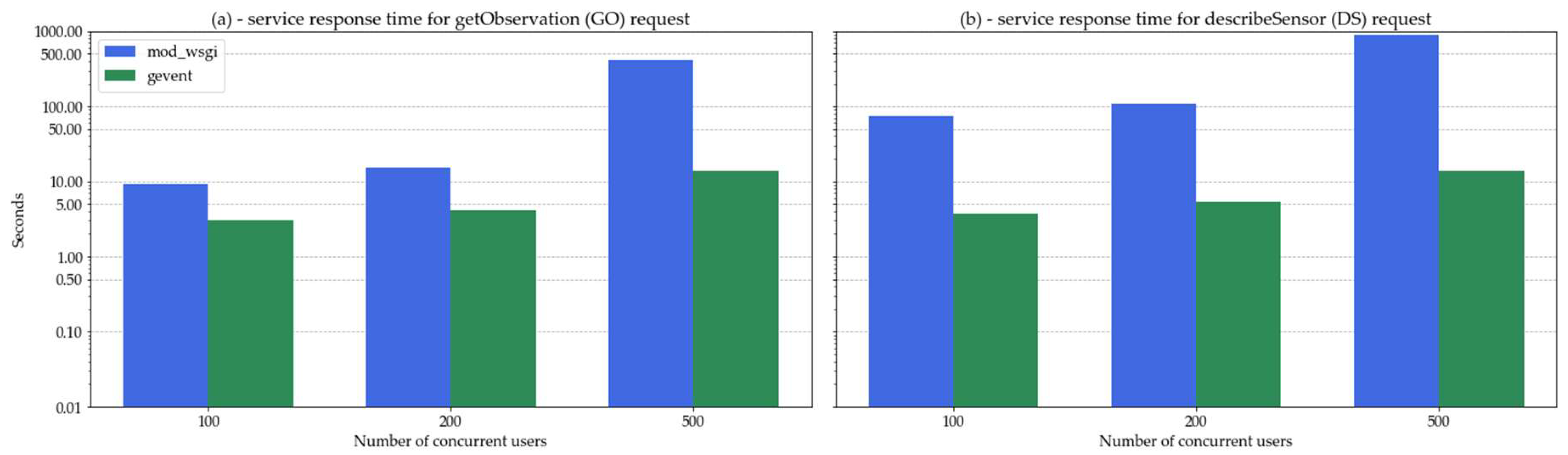
3.3. Case C: Springs and Wells Monitoring Network in Ticino

In case C, the insertObservation operation has not been included in the test since the data registration frequency is 1 month and thus the frequency of this operation is clearly negligible with respect to the others. As a result, only the data consumer user profile has been tested in case C. In Figure 5 the average response times for different requests and concurrent users and WSGI application are represented in logarithmic scale.

Table 15. Requests per second (total and for different SOS request) with different concurrent data consumers and WSGI applications for the test case of a large size monitoring network (case C). Rate of failure (ρ) is reported when errors have been detected. Values reported as n.a. indicates that it was not possible to execute the test for that request and users combination.

Request	GC	DS	GO	TOT
100m	0.05	0.16	2.23	2.44
200m	0.09	0.29	3.98	4.36
500m	0.20 (ρ = 45.4%)	0.38 (ρ = 77.0%)	0.13 (ρ = 74.3%)	0.71 (ρ = 74.3%)
1000m	3.33 (ρ = 97.5%)	0.58 (ρ = 99.1%)	n.a.	3.92
2000m	10.27 (ρ = 99.9%)	0.01 (ρ = 100%)	n.a.	10.28
100g	0.08 (ρ = 4.8%)	0.30	4.66	5.03
200g	0.14 (ρ = 13.3%)	0.47	7.21	7.82
500g	0.21 (ρ = 64.8%)	0.22	2.79	3.22
1000g	2.09 (ρ = 100%)	n.a.	n.a.	2.09
2000g	9.67 (ρ = 100%)	n.a.	n.a.	9.67

shows the service loads of the tests, in terms of requests per seconds and rate of filure. gevent registers a higher rate of failure but in the cases of no-error performed much faster (83 times in average) than mod_wsgi in registered response-time.

In the pipe of the data consumer request workflow (see Figure 2), GC is a blocking request. In fact, if no answer is received the user has no information to perform either the exploration of specific sensors or any request for data. The requests produced unacceptable long response time (see Figure 5): close to 10 min in average for 100 and 200 concurrent users and rising up to about 26 min with 500 users. For higher concurrent users the time to obtain a response continues to increase with mod_wsgi while gevent was not able to provide any response in the timeframe of the test (see n.a. values in Table 15).

With both mod_wsgi and gevent the percentage of GC response failures for 500 users is about 50% and very close to 100% for 1000 and 2000 users. These percentages of error are invalidating the test results for the DS and GO requests for 500, 1000 and 2000 and thus they are omitted in Figure 6.

In both these cases gevent registered faster responses. For example, it was 20 times faster for DS100 and DS200 (5 sec vs 100 sec) and 2 times faster for GO100 and GO200. In the case of DS500 users gevent over performed mod_wsgi of 64 times (13 vs 887 seconds) while in the case of GO500 of 30 times.

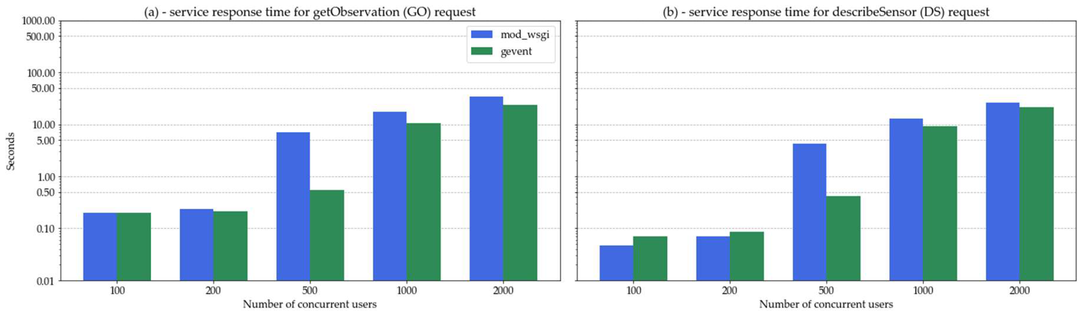
Due to the previously discussed bias introduced by the high error rate on the service testing, this load testing has been re-executed excluding the GC requests. In this case, the list of procedures and observed properties were hardcoded in the testing scripts. This is to overcome the lack of information for performing DS and GO requests. Results of this further test are reported in

Table 16. Requests per second (total and for different SOS request) with different concurrent data consumers and WSGI applications for the test case of a large size monitoring network (case C) excluding the getObservation request. Rate of failure (ρ) is reported when errors have been detected.

Request	DS	GO	TOT
100m	0.39	7.39	7.78
200m	0.78	14.71	15.49
500m	1.32	23.08	24.40
1000m	1.71 (ρ = 0.14%)	29.16 (ρ = 0.22%)	30.87
2000m	2.40 (ρ = 5.90%)	36.64 (ρ = 7.52%)	39.05
100g	0.39	7.40	7.79
200g	0.78	14.76	15.54
500g	1.93	35.55	37.47
1000g	2.01	33.99	35.99
2000g	2.50	38.97	41.47

and Figure 7.

The response errors drastically drop down and the executed requests per seconds increased. In average, not considering tests with failures, gevent registered two times faster responses, ratio that became more important with higher concurrent users (for example 10 time faster in DS and GO 500 tests). In

Table 17. Percentage of describeSensor requests completed within given times (in seconds) for the different configuration of concurrent users and WSGI server (case C).

Request	50%	66%	75%	80%	90%	95%	98%	99%	100%
DS100g	0.04	0.05	0.07	0.10	0.18	0.23	0.33	0.36	0.68
DS200g	0.05	0.08	0.11	0.14	0.20	0.26	0.35	0.41	0.83
DS500g	0.21	0.34	0.46	0.56	0.92	1.50	2.70	3.80	6.75
DS1000g	10.00	13.00	14.00	15.00	16.00	17.00	18.00	18.00	20.38
DS2000g	22.00	28.00	31.00	32.00	36.00	39.00	46.00	50.00	66.44
DS100m	0.04	0.04	0.05	0.05	0.08	0.11	0.17	0.21	0.49
DS200m	0.04	0.06	0.09	0.10	0.16	0.22	0.30	0.35	0.67
DS500m	4.90	6.00	6.60	7.00	8.10	8.80	9.60	10.00	11.19
DS1000m	16.00	17.00	17.00	18.00	19.00	20.00	21.00	22.00	40.70
DS2000m	29.00	33.00	36.00	38.00	48.00	53.00	59.00	63.00	107.97

and

Table 18. Percentage of getObservation requests completed within given times (in seconds) for the different configuration of concurrent users and WSGI server (case C).

Request	50%	66%	75%	80%	90%	95%	98%	99%	100%
GO100g	0.18	0.20	0.23	0.25	0.30	0.35	0.43	0.48	1.06
GO200g	0.19	0.23	0.26	0.28	0.34	0.40	0.48	0.54	1.42
GO500g	0.35	0.48	0.60	0.70	1.10	1.60	2.80	3.60	7.05
GO1000g	11.00	13.00	15.00	15.00	16.00	17.00	18.00	18.00	21.98
GO2000g	25.00	29.00	32.00	33.00	36.00	40.00	48.00	51.00	68.49
GO100m	0.18	0.20	0.22	0.24	0.29	0.33	0.39	0.43	0.88
GO200m	0.21	0.25	0.29	0.31	0.39	0.47	0.59	0.68	1.47
GO500m	7.90	8.90	9.70	10.00	12.00	12.00	13.00	13.00	15.56
GO1000m	19.00	20.00	21.00	21.00	23.00	23.00	25.00	25.00	42.26
GO2000m	35.00	39.00	42.00	44.00	51.00	56.00	61.00	65.00	112.16

the percentage of DS and GO requests completed within given times for the different configuration of concurrent users and WSGI server are reported.

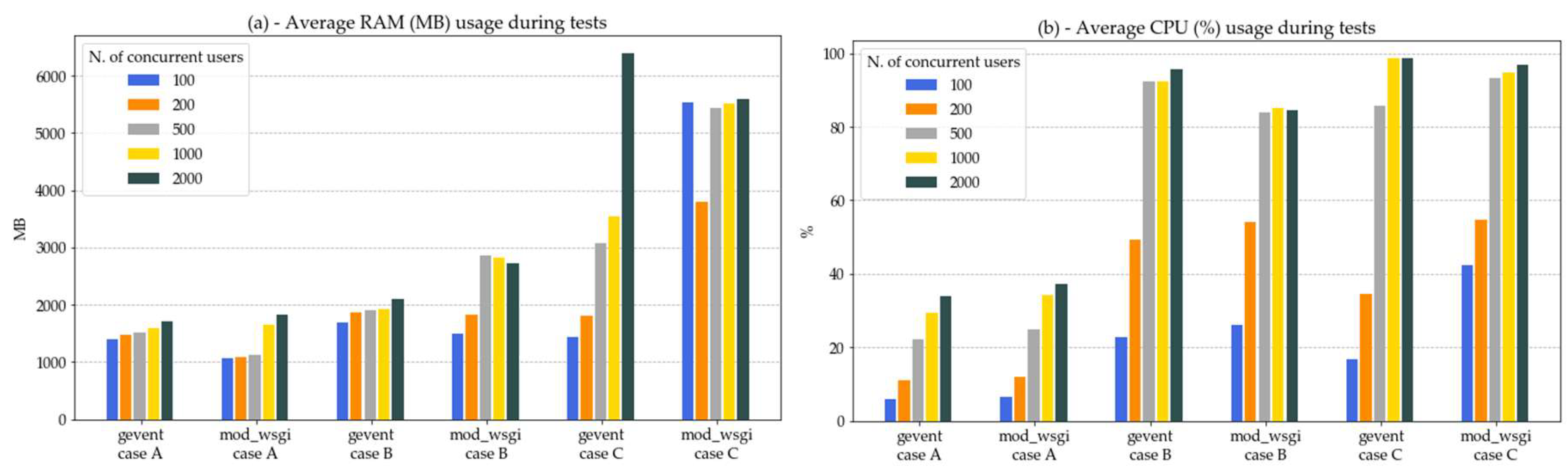
3.4. Hardware Performance

The system performance metrics have been monitored and recorded during the test execution by means of dstat. As illustrated in Figure 8, only a minimal part of the 32GB available were used. In case A, it was limited to less than 2 GB; in case B less than 3 GB and in case C it reached a maximum of 6.4 GB.

The usage rate of the 6 available processors during the tests are plotted in Figure 8. In case A it never exceeded the 40%. In case B in tests with more than 200 users it gets close to 90%: about 95% for gevent and 85 for mod_wsgi. In case C processors are almost saturated with more than 500 users.

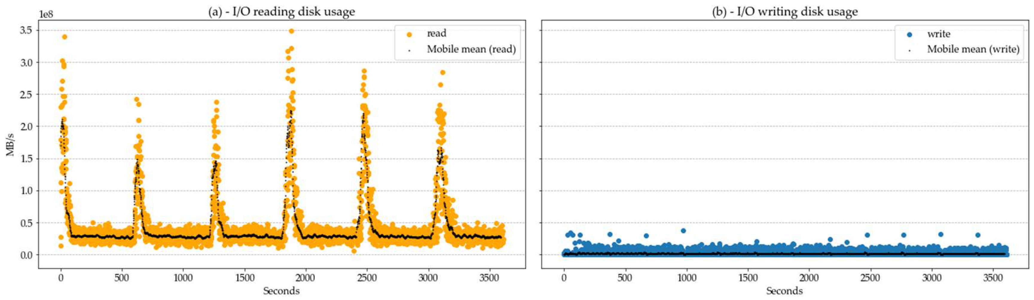
Along all the tests, the registered disk I/O speed in writing had a mean of 2,049.32 ± 1,915.18 KB/s and a maximum of 77,744.00 KB/s. In reading an average of 32,694.31 ± 11,609.67 KB/s and a maximum of 477,288.00 KB/s. In all the cases below of the maximum SSD speed of 520,000 KB/s. The temporal behaviour of the I/O write speed parameter shows, in all the tests, an almost constant rate interleaved by high peaks in correspondence of insertObservation requests. The I/O read speed is always regular. As a representative example of this behaviours, the test on case B with 500 users and gevent is illustrated in Figure 9.

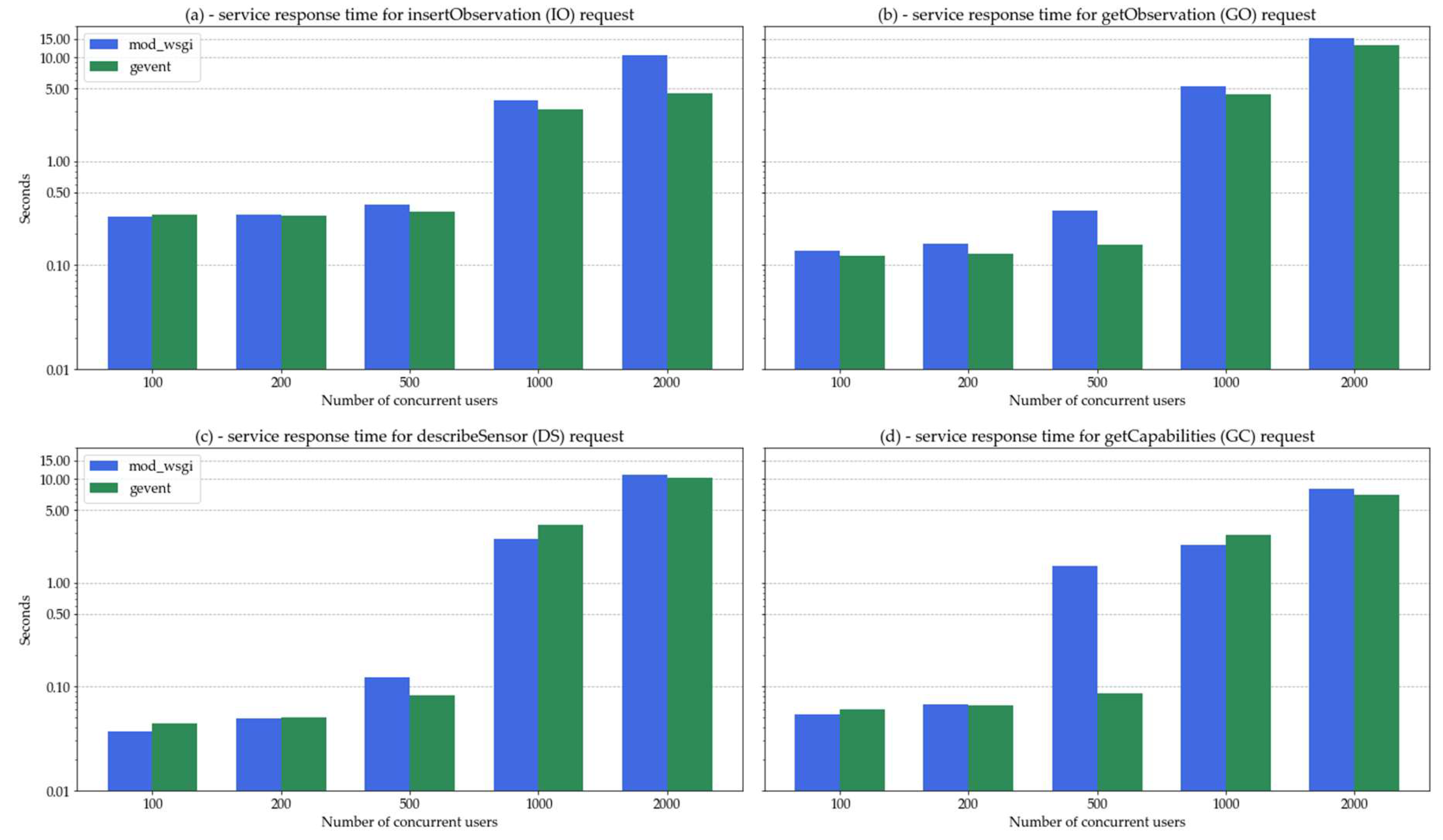
3.5. WSGI Servers Performance

In the experiments two different WSGI server application were used and its response based on test case and request is reported in the previous section. In Figure 10 the average response time difference between gevent and mod_wsgi WSGI servers registered during the load testing in case A, B and C with 100, 200, 500 and 1000 users is represented. Tests were failures were registered are not considered as they may affect the performance registered. In case C getCapabilities (GC) and insertObservations(IO) were not tested.

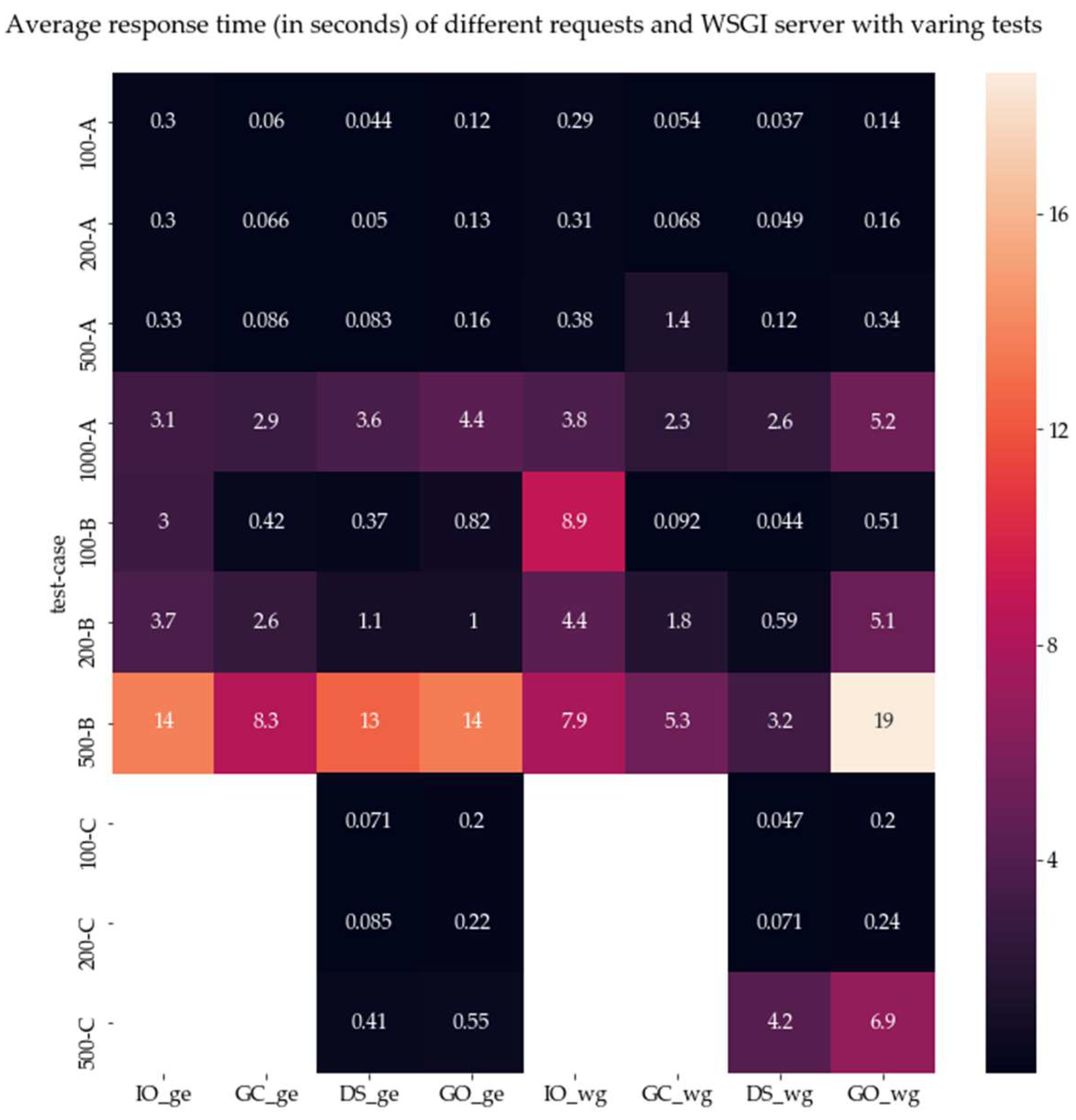
In Figure 11, the average response times for the different tests are illustrated to provide a general overview of all the tests. In this image, as discussed previously in the paper, the test cases that registered errors are omitted since they could have affected the actual response time.

4. Discussion

As described in the methodology chapter, in this sections the results are evaluated with respect to the Quality of Services (QoS) defined by INSPIRE in the requirements for network services and respective Technical Guidance (TG) documents.

If we compare the SOS’s getCapabilities and describeSensor requests with INSPIRE’s Get Download Service Metadata, we can observe that in case A, mid-size monitoring system, istSOS is on average satisfying the 10 seconds response time limits for all the concurrency scenarios. If we look at the percentage of requests exceeding this limit we can clearly see that this performance is guaranteed to 100% only up to 500 concurrent users, 98% up to 1000 users and only up to 50% with 2000 users. In the case B, characterized by a big number of observations, the conformance with this limit is never guaranteed to 100% if gevent is used. Nevertheless, with the exception of a low percentage of requests (from 10% to 1%) it is satisfied with up to 200 users using gevent and 500 users using mod_wsgi. In case C, characterized by big number of sensors, in the test that excluded the getCapabilities request due to its high errors, the performance limit is satisfied with up to 500 users using both the WSGIs: only 1% of the responses in DS500m exceeded by the 12% the limit.

Similarly, if we compare the SOS’s getObservation request to the INSPIRE’s Get Spatial Data Set request we can see that istSOS satisfies the performance limits set by INSPIRE for data recovery in all load scenarios in case A, up to 1000 users. In the GO2000g scenario only 1% of the requests exceeded the limit, while in the GO2000m scenario only 80% of the requests were below the 30 seconds. In case B, the service fulfils the INSPIRE performance requirements for scenarios of 200 and 500 concurrent users regardless the WSGI used. With 500 users it is mostly satisfied (up to 95% of the requests with gevent and up to 90% with mod_wsgi) while with 1000 and 2000 it is never fulfilled. In the case C with GC excluded, the limit is fulfilled up to 1000 users with the exception of the 1% of requests in GO1000m scenario. With 2000 users only gevent partially satisfied the limit and only for the 66% of the requests.

There is no equivalent in INSPIRE services for insertObsrvation but being a transactional request to dynamically add data to the system we could, as a first instance, use the same 30 seconds limit used for data requests. Under this assumption, we can see from the load test results that istSOS satisfies the INSPIRE’s performance limits in all the load scenarios of case A, except for the 10% of requests in scenario IO2000m. In the case B, this limit is met only up to 500 users and in the case of IO500g up to 90% of the responses. With mod_wsgi and 1000 and 2000 users only the 80% of the responses are below the limit and with gevent only for 1000 users the system was able to keep the response time in the 66% of within the INSPIRE performance limit.

Since the tests have been performed for a short period of time, it is not possible to draw final conclusions about the robustness of istSOS, intended as the ability of the service to function correctly even in presence of errors. However, during the entire testing periods we have registered the absence of any downtime despite the presence of errors. The availability during the test period was therefore 100% since the service was always up. Nevertheless, the user perceived availability of the service is strongly impacted by the rate of failure. In this regard, if we consider the errors as service unavailability, istSOS showed that if gevent is used as WSGI server, the 99% of availability is guarantee in both case A and B, while for case C it is guarantee with the exception of the getCapabilities request. Results obtained with mod_wsgi are in average of worst quality, in fact they satisfy the availability criterion only up to 1000 simultaneous users in case A and 500 in case B and C.

The capacity limit set by the TG for INSPIRE download services, identifying the load scenario that the service should be able to sustain providing a compliant performance, are 10 requests per seconds (req/sec). The technical guidelines also allowed the server not to respond in orderly fashion to requests exceeding 50 simultaneous requests; in the current study this condition is ignored since the scope of this work is to test the service under high peak usage conditions. From the performance results, we have seen that the case A satisfies the performance criteria up to 1000 users, which means a capacity of 56.38 and 53.98 req/sec respectively with mod_wsgi and gevent (see Table 5). In the case B the performance limits are met at maximum with 200 users, which identify for mod_wsgi 11.89 req/sec and for gevent 15.42 req/sec (see Table 10). For case C (ex-cluding GC requests) the performance limits are respected up to 500 users, which registered 24.40 and 37.47 req/sec (see Table 15).

Looking at the usage of the hardware resources during the tests execution, we can see that the configuration of the server was adequate to support the tested cases. In fact, with the exception in few cases of CPU usage (with 2000 concurrent users), the physical server limits were not reached. It is particularly interesting to see how the disk I/O is particularly stressed when the sensors register new observations (insertObservation requests). In fact, contrary of what can be expected, the data retrieval is using less I/O than the data insertion. To better understand this apparently strange behaviours the database log files of case B with 500 concurrent users were analysed as a representative case. The total time of the queries for each specific SOS request has been evaluated and is reported in

Table 19. Database queries time statistics, registered in test case B and 500 concurrent users, aggregated for SOS request type (IO=insertObservation, GC=getCapabilities, DS=describeSensor, GO=getObservation).

Request	Mean (sec)	Min (sec)	Max (sec)	Total (hours)
IO	13.46	0. 784	45.022	2.993
GC	0. 718	0.017	9.173	0.110
DS	1.044	0.002	34.570	0.935
GO	1.807	0.416	46.088	15.751

. From these statistics we can clearly see how the execution of an IO request is in average a level of magnitude higher of the GO.

The main reason for the difference is due to the data integrity checks that the software performs before inserting new data. In fact, at each IO request before inserting the data, istSOS:

• authenticates the sensor trough a unique identifier provided at registration;
• verifies that the properties observed are exactly those specified at sensor registration.
• verifies that the new data have later observation time then the latest registered observation for the same sensor;

These three operations take 98.8% on average of the total duration of the request’s queries, and the latest check is particular slow because it executes a “SELECT MAX()” query type over the time-series. The queries of a GO request, which has no data integrity checks but needs to compose the XML response in memory, cost 13.3% on average of the queries of a GO request.

Since we recognize that, in general, hardware configuration affects the results in load testing experiments, we tried to minimize this impact by avoiding the use of virtual systems, using a high-speed band and running the requests from a physically different machine. While we cannot state that the hardware did not affected the results we can safely assume that it does not play a crucial role in this tests. In fact the recorded hardware usage showed that the system was adequately dimensioned with the RAM that were never fully used and the CPU that only in the case C with 1000 and 2000 users was close (but below) to 100%.

Analysing Figure 10, we can see that in general gevent and mod_wsgi, the two WSGI server we have tested, are equivalent for low concurrency. However, for the getObservations request gevent is faster and presents the higher performance differences with respect to the mod_wsgi. On the contrary, in case B (larger number of observations) with 500 concurrent users the performance of mod_wsgi outperformed gevent in all the other requests (DS, GC and IO). A possible motivation for this behaviour could reside in a better capacity of gevent, that is based on co-routines, in handling I/O blocking operations like the GO request, while mod_wsgi using a multi-processes and multi-thread approach execute faster requests like GC, IO and DS without interferences of I/O blocking requests.

The three varying parameters of tests are: number of sensors, number of stored observations and number of concurrent users. From the experiments, it is clear that the increase in size of the observations and of the sensors, from case A (105 million of observations and 20 sensors) to case B (1.7 billions of observations and 130 sensors), produce slower responses regardless of the WSGI server used. Similarly, the increase of size in the sensors and reduction of observations, from case A (20 sensors and 105 million of observations) and case C (5100 sensors and 122 thousand observations) produced slower response time. This indicates that both the increase of stored historical observations and the number of deployed sensors negatively affect the istSOS performance. While it is not possible to separate the negative contribution on performance of the two components it is clear that the number of stored data has a greater negative impact than the number of sensors. In fact, from case A to case C with respect to case A to case B sensors increase of 50 times while observations diminish of 500 time and performance degrades of 5 times.

5. Conclusions

With the presented research the authors have conducted a quantitative test of the istSOS software solution, which implements the SOS standard from the OGC under different conditions. The objective of the test was to understand the capabilities of the software, under ordinary installation, to meet the requirements of interoperable temporal and real-time GIS posed by the current state of the art in environmental modelling, visualization and Earth observation. To this end, the test analysed the service behaviour under different realistic monitoring networks, number of concurrent users and WSGI server type. The synthetic networks used in the test were inspired by existing deployed systems and specifically mimicked a regular monitoring network with 20 sensors and 100 million observations, a monitoring network with more station and data, composed by 130 sensors and 1.7 billion measures, and a monitoring network with a large number of sensors (5100) and limited data (1.7 million). Scenarios with 100, 200, 500, 1000 and 2000 concurrent users were tested for each network and for two different WSGI server (mod_wsgi and gevent). The monitored and registered service metrics for each testing scenarios and different SOS requests were: served requests per second, response times and errors. Additionally, the server resource consumption in term of CPU, RAM and I/O has been monitored and registered.

The presented results show that istSOS is able to meet the INSPIRE requirements for a download service in terms of quality of service with some limitations, in case of high number of concurrent users. This limit is due to the demonstrated degradation of the software performance with spatial scaling (increasing number of deployed sensors) and temporal scaling (increasing length of time-series). In particular, in case of spatial scaling low performance, istSOS produced a large amount of errors because of the large size of the getCapabilities response document which overloaded the service and consequently registered a large amount of time-out failures. This study has also demonstrated that gevent produces less errors than mod_wsgi and is able to have higher throughput (executed requests per second). Specifically, gevent showed better performance in dispatching observations by executing getObservations requests while mod_wsgi is better in dispatching metadata (getCapabilities and describeSensors requests).

The results demonstrate also that with an high number of sensors and high concurrency the getCapabilities request undermine the correct working of istSOS. In fact, its extremely high response time causes timeout errors that block the server from executing other requests.

The study shows that istSOS’ strategy to implement data integrity checks before registering a new observation has a great cost. This cost may represent a great obstacle in case of monitoring systems characterized by high-frequency or high-number of sensors and requiring very fast data insertion to satisfy the real time geospatial applications needs.

As a general remark, the authors underline the fact that the QoS limits set for INSPIRE’s download service are designed to serve data to generally support the formulation, implementation, monitoring and evaluation of policies and activities, which have a direct or indirect impact on the environment. In this regard, this research has demonstrated that istSOS is suitable for most of the scientific or operational applications where data are accessed by tens of users with peaks of one hundred in emergency cases [14,39]. However, it also demonstrated that its capacity of scaling with increasing size of monitoring network, either in term of number of stored observations or sensors, is limited. The degrading performances make istSOS in a standalone installation not capable of providing a sufficient quality of service for Internet of Things (IoT) applications where thousands of concurrent users, directly accessing the data, and applications with thousands of connected sensors are expected.

From the software development perspective, the test has shown the challenges to be addressed by future versions: improve the response speed and the software capacity. The first would require some code optimisation, particularly to speed up the query execution time for data integrity checks. The latter would require the implementation of a strategy to scale istSOS at the application level. this could be addressed in future istSOS versions by exploring micro-services architecture and asynchronous programming.

References

1. Gore, A. The digital earth. Aust. Surv. 1998, 43, 89–91. [Google Scholar] [CrossRef]
2. Goodchild, M.F. The use cases of digital earth. Int. J. Digit. Earth 2008, 1, 31–42. [Google Scholar] [CrossRef]
3. Butler, D. Virtual globes: The web-wide world. Nature 2006, 439, 776–778. [Google Scholar] [CrossRef] [PubMed]
4. Patterson, T.C. Google Earth as a (Not Just) Geography Education Tool. J. Geogr. 2007, 106, 145–152. [Google Scholar] [CrossRef]
5. Bell, D.G.; Kuehnel, F.; Maxwell, C.; Kim, R.; Kasraie, K.; Gaskins, T.; Hogan, P.; Coughlan, J. NASA World Wind: Opensource GIS for Mission Operations. In Proceedings of the 2007 IEEE Aerospace Conference, Big Sky, MT, USA, 3–10 March 2007; pp. 1–9. [Google Scholar]
6. CesiumJS—Geospatial 3D Mapping and Virtual Globe Platform. Available online: https://cesiumjs.org/ (accessed on 1 March 2019).
7. Keysers, J.H. Review of Digital Globes 2015: Australia and New Zealand Cooperative Research Centre for Spatial Information. 2015, p. 24. Available online: https://www.crcsi.com.au/assets/Resources/Globe-review-paper-March-2015.pdf (accessed on 22 October 2019).
8. Liu, X.; Wang, X.; Wright, G.; Cheng, J.C.P.; Li, X.; Liu, R. A State-of-the-Art Review on the Integration of Building Information Modeling (BIM) and Geographic Information System (GIS). ISPRS Int. J. Geo-Inf. 2017, 6, 53. [Google Scholar] [CrossRef]
9. INSPIRE|Welcome to INSPIRE. Available online: https://inspire.ec.europa.eu/ (accessed on 1 March 2019).
10. GEO. Available online: http://www.earthobservations.org/index.php (accessed on 1 March 2019).
11. enviroGRIDS. Available online: http://www.envirogrids.net/ (accessed on 1 March 2019).
12. ACQWA. Available online: http://www.acqwa.ch/ (accessed on 1 March 2019).
13. Copernicus. Available online: https://www.copernicus.eu/en (accessed on 1 March 2019).
14. Giuliani, G.; Lacroix, P.; Guigoz, Y.; Roncella, R.; Bigagli, L.; Santoro, M.; Mazzetti, P.; Nativi, S.; Ray, N.; Lehmann, A. Bringing GEOSS Services into Practice: A Capacity Building Resource on Spatial Data Infrastructures (SDI). Trans. GIS 2017, 21, 811–824. [Google Scholar] [CrossRef]
15. Na, A.; Priest, M. OpenGIS Sensor Observation Service (SOS) Encoding Standard; 616 OpenGIS standard 06-009r6; 616 OpenGIS Standard: 2007. Available online: https://www.opengeospatial.org/standards/sos (accessed on 22 October 2019).
16. Bröring, A.; Stasch, C.; Echterhoff, J. OGC® Sensor Observation Service Interface Standard. 2012. Available online: https://www.opengeospatial.org/standards/sos (accessed on 22 October 2019).
17. Liang, S.; Huang, C.-Y.; Khalafbeigi, T. OGC SensorThings API Part 1: Sensing. 2016. Available online: https://www.opengeospatial.org/standards/sensorthings (accessed on 22 October 2019).
18. Bierkens, M.F.P.; Bell, V.A.; Burek, P.; Chaney, N.; Condon, L.E.; David, C.H.; de Roo, A.; Döll, P.; Drost, N.; Famiglietti, J.S.; et al. Hyper-resolution global hydrological modelling: What is next? Hydrol. Process. 2015, 29, 310–320. [Google Scholar] [CrossRef]
19. Chatzikostas, G.; Boskidis, I.; Symeonidis, P.; Tekes, S.; Pekakis, P. Enorasis. Procedia Technol. 2013, 8, 516–519. [Google Scholar] [CrossRef] [Green Version]
20. Rossetto, R.; De Filippis, G.; Borsi, I.; Foglia, L.; Cannata, M.; Criollo, R.; Vázquez-Suñé, E. Integrating free and open source tools and distributed modelling codes in GIS environment for data-based groundwater management. Environ. Model. Softw. 2018, 107, 210–230. [Google Scholar] [CrossRef]
21. Godish, T.; Davis, W.T. Air Quality. Available online: https://www.crcpress.com/Air-Quality/Godish-Davis-Fu/p/book/9781466584440 (accessed on 1 March 2019).
22. Liu, J.; Mooney, H.; Hull, V.; Davis, S.J.; Gaskell, J.; Hertel, T.; Lubchenco, J.; Seto, K.C.; Gleick, P.; Kremen, C.; et al. Systems integration for global sustainability. Science 2015, 347, 1258832. [Google Scholar] [CrossRef] [Green Version]
23. Pearlman, J.; Jirka, S.; Rio, J.D.; Delory, E.; Frommhold, L.; Martinez, S.; O’Reilly, T. Oceans of Tomorrow sensor interoperability for in-situ ocean monitoring. In Proceedings of the OCEANS 2016 MTS/IEEE Monterey, Monterey, CA, USA, 19–23 September 2016; pp. 1–8. [Google Scholar]
24. Leppelt, T.; Gebbert, S. A GRASS GIS based Spatio-Temporal Algebra for Raster-, 3D Raster- and Vector Time Series Data. In Proceedings of the EGU General Assembly Conference Abstracts, Vienna, Austria, 12–17 April 2015; Volume 17, p. 11672. [Google Scholar]
25. Gong, J.; Geng, J.; Chen, Z. Real-time GIS data model and sensor web service platform for environmental data management. Int. J. Health Geogr. 2015, 14, 2. [Google Scholar] [CrossRef] [PubMed]
26. Roberts, D.; Dunn, B.; Mueller, N. Open Data Cube Products Using High-Dimensional Statistics of Time Series. In Proceedings of the IGARSS 2018—2018 IEEE International Geoscience and Remote Sensing Symposium, Valencia, Spain, 22–27 July 2018; pp. 8647–8650. [Google Scholar]
27. Gorelick, N.; Hancher, M.; Dixon, M.; Ilyushchenko, S.; Thau, D.; Moore, R. Google Earth Engine: Planetary-scale geospatial analysis for everyone. Remote Sens. Environ. 2017, 202, 18–27. [Google Scholar] [CrossRef]
28. Fekete, B.M.; Robarts, R.D.; Kumagai, M.; Nachtnebel, H.-P.; Odada, E.; Zhulidov, A.V. Time for in situ renaissance. Science 2015, 349, 685–686. [Google Scholar] [CrossRef] [PubMed]
29. Famiglietti, J.S.; Cazenave, A.; Eicker, A.; Reager, J.T.; Rodell, M.; Velicogna, I. Satellites provide the big picture. Science 2015, 349, 684–685. [Google Scholar] [CrossRef] [PubMed] [Green Version]
30. Conover, H.; Berthiau, G.; Botts, M.; Goodman, H.M.; Li, X.; Lu, Y.; Maskey, M.; Regner, K.; Zavodsky, B. Using sensor web protocols for environmental data acquisition and management. Ecol. Inform. 2010, 5, 32–41. [Google Scholar] [CrossRef]
31. Su, H.; Houser, P.R.; Tian, Y.; Geiger, J.V.; Kumar, S.V.; Belvedere, D.R. A Land Information Sensor Web (LISW) Study in Support of Land Surface Studies. In Proceedings of the IGARSS 2008—2008 IEEE International Geoscience and Remote Sensing Symposium, Boston, MA, USA, 7–11 July 2008; Volume 5, p. V-144. [Google Scholar]
32. Lauterjung, J.; Rudloff, A. GITEWS—The German-Indonesian Tsunami Early Warning System. In Proceedings of the AGU Fall Meeting Abstracts, San Francisco, CA, USA, 5–9 December 2005; Volume 13, p. U13A-06. [Google Scholar]
33. Cannata, M.; Antonovic, M. Sensor Observations Service for Environmentally Opti-mizing Irrigation: istSOS within the ENORASIS Example. Int. J. Geoin-Form. 2015, 11, 1–8. [Google Scholar]
34. Poorazizi, M.E.; Liang, S.H.L.; Hunter, A.J.S. Testing of Sensor Observation Services: A Performance Evaluation. In Proceedings of the First ACM SIGSPATIAL Workshop on Sensor Web Enablement, Redondo Beach, CA, USA, 6 November 2012; ACM: New York, NY, USA, 2012; pp. 32–38. [Google Scholar]
35. 52°North Sensor Observation Service (SOS) Home Page. Available online: https://52north.org/software/software-projects/sos/ (accessed on 22 October 2019).
36. Mapserver project Home Page. Available online: https://mapserver.org/ogc/sos_server.html (accessed on 22 October 2019).
37. Zhou, Y.; Xie, H. The integration technology of sensor network based on web crawler. In Proceedings of the 2015 23rd International Conference on Geoinformatics, Wuhan, China, 19–21 June 2015; pp. 1–7. [Google Scholar]
38. istSOS project Home Page. Available online: http://istsos.org/ (accessed on 22 October 2019).
39. Cannata, M.; Antonovic, M.; Molinari, M.; Pozzoni, M. istSOS, a new sensor observation management system: Software architecture and a real-case application for flood protection. Geomat. Nat. Hazards Risk 2015, 6, 635–650. [Google Scholar] [CrossRef]
40. Eby, P.J. PEP 333—Python Web Server Gateway Interface v1.0. Available online: https://www.python.org/dev/peps/pep-0333/ (accessed on 1 March 2019).
41. Isufi, F.; Isufi, A.; Bulliqi, S. Development of NASA world wind based application to display sensors observation according to istsos platform. In Proceedings of the 14th SGEM GeoConference on Informatics, Geoinformatics and Remote Sensing, Albena, Bulgaria, 17–26 June 2014; Volume 1, pp. 587–592. [Google Scholar]
42. Munoz, C.A.; Brovelli, M.A.; Corti, S.; Micotti, M.; Sessa, S.; Weber, E. A FOSS approach to Integrated Water Resource Management: The case study of Red-Thai Binh rivers system in Vietnam. Geomat. Workb. 2015, 12, 471–476. [Google Scholar]
43. Eberle, J.; Urban, M.; Homolka, A.; Hüttich, C.; Schmullius, C. Multi-Source Data Integration and Analysis for Land Monitoring in Siberia. In Novel Methods for Monitoring and Managing Land and Water Resources in Siberia; Mueller, L., Sheudshen, A.K., Eulenstein, F., Eds.; Springer International Publishing: Cham, Switzerland, 2016; pp. 471–487. ISBN 978-3-319-24409-9. [Google Scholar]
44. Menasce, D.A. Load testing of Web sites. IEEE Internet Comput. 2002, 6, 70–74. [Google Scholar] [CrossRef]
45. Heyman, H. Implementing Dynamic Allocation of User Load in a Distributed Load Testing Framework. Bachelor Thesis, Uppsala University, Uppsala, Finland, 2013. [Google Scholar]
46. Cannata, M.; Antonovic, M.; Molinari, M.E. Load testing of HELIDEM geo-portal: An OGC open standards interoperability example integrating WMS, WFS, WCS and WPS. Int. J. Spat. Data Infrastruct. Res. 2015, 9, 107–130. [Google Scholar] [CrossRef]
47. Dstat command manual Home Page. Available online: http://linux.die.net/man/1/dstat (accessed on 22 October 2019).
48. Osservatorio Ambientale della Svizzera Italiana (OASI) Home Page. Available online: http://www.oasi.ti.ch/web/dati/aria.html (accessed on 22 October 2019).
49. Nielsen, A. Python Programming—Web Serving. 2013; Available online: http://www2.imm.dtu.dk/pubdb/views/edoc_download.php/5946/pdf/imm5946.pdf (accessed on 22 October 2019).
50. Fonseca, A.; Rafael, J.; Cabral, B. Eve: A Parallel Event-Driven Programming Language. In Euro-Par 2014: Parallel Processing Workshops; Lopes, L., Žilinskas, J., Costan, A., Cascella, R.G., Kecskemeti, G., Jeannot, E., Cannataro, M., Ricci, L., Benkner, S., Petit, S., et al., Eds.; Springer International Publishing: Cham, Switzerland, 2014; pp. 170–181. [Google Scholar]
51. Piël, N. Benchmark of Python WSGI Servers. Available online: http://www.voidcn.com/article/p-sytdrkvi-bex.html (accessed on 1 March 2019).
52. Multi-Processing Modules (MPMs)—Apache HTTP Server Version 2.4. Available online: https://httpd.apache.org/docs/2.4/mpm.html (accessed on 19 July 2019).
53. Han, W.; Di, L.; Yu, G.; Shao, Y.; Kang, L. Investigating metrics of geospatial web services: The case of a CEOS federated catalog service for earth observation data. Comput. Geosci. 2016, 92, 1–8. [Google Scholar] [CrossRef]
54. Seip, C.; Bill, R. Evaluation and Monitoring of Service Quality: Discussing Ways to Meet INSPIRE Requirements. Trans. GIS 2016, 20, 163–181. [Google Scholar] [CrossRef]
55. Giuliani, G.; Dubois, A.; Lacroix, P. Testing OGC Web Feature and Coverage Service performance: Towards efficient delivery of geospatial data. J. Spat. Inf. Sci. 2013, 2013, 1–23. [Google Scholar] [CrossRef]
Figure 1. Graphical user interface of the istSOS software. At the top-left a screenshot of the administration interface to register a new sensor to the monitoring network: specifics buttons opens new interface for Web service settings and configurations. At the top-right, the data editor interface to manipulate and validate data. At the bottom, the data viewer interface to explore data in space and time by observed properties.
Ijgi 08 00467 g001
Figure 2. Users of a Sensor Observation Service and workflow of interactions with the server for information access.
Ijgi 08 00467 g002
Figure 3. Service response time for different Sensor Observation Service (SOS) requests in test case A (Air-quality Monitoring Network): insertObservation request in plot (a), getObservation request in plot (b), describeSensor request in plot (c) and getCapabilities request in plot (d).
Ijgi 08 00467 g003
Figure 4. Service response time in logarithmic scale for different SOS requests in test case B (Swiss Meteorological Monitoring Network): insertObservation request in plot (a), getObservation request in plot (b), describeSensor request in plot (c) and getCapabilities request in plot (d).
Ijgi 08 00467 g004
Figure 5. Service response time for the getCapabilities SOS requests in test case C (Springs and Wells Monitoring Network in Ticino)
Ijgi 08 00467 g005
Figure 6. Service response time for the getObservation (a) and describeSensor (b) SOS requests in test case C (Springs and Wells Monitoring Network in Ticino)
Ijgi 08 00467 g006
Figure 7. Service response time for the getObservation (a) and describeSensor (b) SOS requests in test case C (Springs and Wells Monitoring Network in Ticino) after excluding getCapabilities requests from the test.
Ijgi 08 00467 g007
Figure 8. Average RAM (a) and processors (CPU) (b) usage during different test cases and concurrent users
Ijgi 08 00467 g008
Figure 9. Disk usage in reading (a) and writing (b) during the test case B with 500 concurrent users.
Ijgi 08 00467 g009
Figure 10. Average response time difference (in seconds) between gevent and mod_wsgi WSGI servers registered during the load testing in case A, B and C with 100, 200, 500 and 1000 users. Positive values indicate that mod_wsgi was slower; on the contrary, negative values indicate that gevent was faster.
Ijgi 08 00467 g010
Figure 11. Average response time for different requests (IO, GC, DS, GO) and WSGI servers (ge = gevent and wg = mod_wsgi) versus different test cases characterized by different concurrent users (100, 200, 500, 1000) and monitoring networks (A = small size, B = large number of observations, C = large number of sensors).
Ijgi 08 00467 g011