Machine Learning Methods for Classification of the Green Infrastructure in City Areas

Abstract

Rapid urbanization in cities can result in a decrease in green urban areas. Reductions in green urban infrastructure pose a threat to the sustainability of cities. Up-to-date maps are important for the effective planning of urban development and the maintenance of green urban infrastructure. There are many possible ways to map vegetation; however, the most effective way is to apply machine learning methods to satellite imagery. In this study, we analyze four machine learning methods (support vector machine, random forest, artificial neural network, and the naïve Bayes classifier) for mapping green urban areas using satellite imagery from the Sentinel-2 multispectral instrument. The methods are tested on two cities in Croatia (Varaždin and Osijek). Support vector machines outperform random forest, artificial neural networks, and the naïve Bayes classifier in terms of classification accuracy (a Kappa value of 0.87 for Varaždin and 0.89 for Osijek) and performance time.

1. Introduction

Since more and more people are living in cities, it has become extremely important to plan and manage green urban areas. Rapid urbanization has resulted in an increase in interest in green urban areas and the question of how green space can benefit cities and their residents [1]. The importance of green urban areas to improvements in quality of life has been discussed in [2,3], where authors have determined the appropriate sizes of green areas in order to improve local climatic conditions. The question of how a combination of trees can optimize thermal comfort under extreme summer conditions was discussed in [4], and the authors concluded that the planning of urban green areas is important to improving the quality of life of cities’ residents. Green infrastructure has been widely explored in order to improve or even achieve sustainability. The authors in [5] discuss the question of how sustainability could be achieved with smart green urban planning and point out that green infrastructure plans are developed at different planning scales. As seen from this short introduction, a number of authors have considered green urban infrastructure planning and they have all come to a similar conclusion: it is important to have quality green urban spaces in cities. In order to successfully plan green urban infrastructure development, it is necessary to have good-quality and up-to-date maps. The authors in [6] found that is difficult to map landscapes using traditional land use and land cover classification techniques because landscape is rapidly changing, but that mapping could be improved with the use of multispectral imagery and machine learning methods. Many studies have been done that explore the possibility of using machine learning methods to map green urban infrastructure. The authors in [7] showed that support vector machines (SVMs) provide high classification accuracy when applied to high-resolution RapidEye satellite imagery. The authors in [8] demonstrate the great potential of neural networks for land cover classification and mapping using Landsat Thematic Mapper imagery. According to [9], the naïve Bayes classifier produces satisfactory land cover classification results when using low-resolution satellite imagery. After different authors had explored the possibilities of different machine learning methods, other authors started to compare these methods to each other. The authors in [10] compared three supervised machine learning algorithms, namely decision tree, random forest, and SVM, using Landsat Thematic Mapper imagery and showed that random forest and SVM achieved similar classification accuracies. The authors in [11] compared artificial neural networks with random forest and SVMs for crop classification using high-resolution RapidEye imagery. They concluded that SVM outperformed the other two machine learning methods. The authors in [12] evaluated the performance of the normal Bayes, K nearest neighbor, random tree, and SVM algorithms for urban pattern recognition from very-high-resolution (WorldView-2, Quickbird, and Ikonos) and medium-resolution (Landsat Thematic Mapper and Landsat Enhanced Thematic Mapper) imagery. SVM and random trees appeared to be the best-performing classifiers on all image types. The authors in [13] compared the SVM, normal Bayes, classification regression tree, and K nearest neighbor algorithms for object-based land cover classification using very-high-resolution imagery and concluded that, based on object-based accuracy assessment, SVM and the normal Bayes algorithm outperformed other two machine learning methods. Most authors compare machine learning methods using very-high- or medium-resolution imagery. Few studies have compared machine learning methods using Sentinel-2 multispectral imagery, as Sentinel-2 has only been active since 2015. The authors in [14] compared the random forest, K nearest neighbor, and SVM algorithms for land cover classification using Sentinel-2 imagery and concluded that SVM provided the best results. The authors in [15] explored how different kernels affect the land cover classification results using Sentinel-2 imagery. They found that the radial basis function produced the highest accuracy and proposed further research using different machine learning methods. This paper is follow-up to a paper published by [15]. Three new machine learning methods will be evaluated and compared to SVM. In order to obtain relevant results, the training areas will remain the same. The novelty of this paper lies in its comparison of four different machine learning methods using Sentinel-2 multispectral imagery of cities. The machine learning methods are used to classify green urban areas, which differs from other studies that focus on either rural areas or forests in towns. We compare SVM to the artificial neural network, naïve Bayes, and random forest machine learning methods. Main purpose of this paper is to perform a comparison between SVM and other machine learning methods in city areas. This paper is written as part of PhD research under the project called Geospatial Monitoring of Green Infrastructure by Means of Terrestrial, Airborne and Satellite Imagery.

SVM is the most commonly used machine learning method [16]. The authors in [16] consider datasets using an optimal hyperplane, and introducing hyperplane was novel for that time. SVM is an abstract machine learning algorithm that learns from a dataset and attempts to generalize and make a correct prediction on new datasets [17]. Kernels are usually used in pairs in SVM modules. Kernel is a function that simulates the projection of the initial data in feature space with higher dimension and in this new space the data are considered as linearly separable. The most commonly used kernels for image processing are the polynomial, radial basis function (RBF), and sigmoid kernels [18]. The authors in [15] discuss the effect of different kernels on supervised classification results. The authors in [15] concluded that the RBF kernel provides the best results with γ = 1 and C = 28, where γ is the free parameter of the radial basis function and C is parameter that allows to trade off training error versus model complexity. They made conclusion based on experiment on two cities in Croatia on Sentinel 2 imagery. Their results for Varaždin and Osijek are presented in

Table 1. The accuracy assessment of Support Vector Machine for Varaždin (left) and Osijek (right) (modified from [15]).

	Varaždin			Osijek
Class No.	C	O	est. Κ	C	O	est. Κ
	0.66	0.00	0.99	0.00	0.19	1.00
2	1.92	0.17	0.97	0.14	9.92	0.99
3	3.40	15.14	0.96	8.09	0.00	0.89
4	11.80	24.95	0.85	6.20	17.38	0.92
5	26.78	12.74	0.66	77.19	51.53	0.21
Κ	0.867978			0.887217

C, comission error; O, omission error.

, and these results will be compared with the results that we obtain in this paper. Class numbers represent different land uses which are according to Corine land cover as it follows. Class number 1 represents Inland waters, class 2 Forests, class 3 Green urban areas, class 4 Arable land and class 5 Urban fabric [19].

Neuron networks date back to the beginning of the 20th century, but their widespread use begins in 1990. The authors in [20] define procedures for neural network machine learning where a known dataset is assigned a weight that is changed in each iteration, which results in higher accuracy. The authors of [21] first mentioned neural networks in 1943 when they published a paper on how neurons might work. Afterwards, not much research was conducted on artificial networks due to limitations in computation power. The breakthrough for artificial neural networks came in 1990 when they were extensively studied. The authors in [22] consider how the depth of the neural network affects the result. They concluded that there remains work to do in order to find the specific parameters that produce maximum accuracy. Given the outputs x_j of the layer n, the outputs y_i of the layer n + 1 in an artificial neural network are calculated as follows:

$$u_i={{\displaystyle \sum }}_j\left(w_{i,j}^{n+1}\ast x_j\right)+w_{i,bias}^{n+1}$$

(1)

$$y_i=f\left(u_i\right)$$

(2)

where w is the weight of each input layer and f is a function. The weights are computed by the training algorithm. There are three different functions:

• the Identity function: $f\left(x\right)=x$;
• the Symmetrical sigmoid: $f\left(x\right)=\beta \ast \left(1-e^{-\alpha x}\right)/\left(1+e^{-\alpha x}\right)$ (the default values are $\beta =1; \alpha =1$); and
• the Gaussian function: $f\left(x\right)=\beta e^{-\alpha x\ast x}$, which is not completely supported at present.

The algorithm takes a training set and multiple input vectors with the corresponding output vectors and iteratively adjusts the weights to enable the network to provide the desired response to the input vectors [23]. The larger the network’s size is, the higher the network’s potential flexibility is. This could affect the error in the training set, which could be made arbitrarily small, but at the same time the network also learns about the noise that is present in the training set, so the error in the test set usually starts increasing after the network’s size reaches the limit [23].

According to [24], the naïve Bayes algorithm is the simplest and most widely tested probabilistic induction method. In this method, each sample has an associated value that represents the probability that the sample will be considered in machine learning. In order to represent knowledge based on the Bayes theorem, [25] proposed Bayesian networks or the naïve Bayes algorithm. A Bayesian network is a graph that shows information flow as directed links between nodes without any loops and consists of nodes and directed links [25,26]. Each node of the network corresponds to a variable and the variables have discrete values [27]. It is typical for the algorithm to learn the relationships and the conditional probability table from training datasets [28]. This simple classification method assumes that feature vectors from each class are normally distributed and not necessarily independently distributed. The whole data distribution function is assumed to be a Gaussian mixture with one component per class. Using the training data, the algorithm estimates mean vectors and covariance matrices for each class, and then uses them for prediction [23].

The author in [29] states that the random forest method combines trees in such a way that each tree depends on a random vector value that is independently sampled and equally distributed for all the in the forest. Random forest is a regression technique that combines numerous decision tree algorithms to classify or predict the value of a variable [29,30]. To avoid correlations between different trees, random forest increases the diversity of the trees by growing them from different training data subsets created through a procedure called bagging [30]. In order to achieve stability, some data may be used more than once while others might never be used. The bagging technique is used to train data by randomly resampling the original datasets with replacements [30]. To reduce the generalization error, random forest uses the best feature/split point within a subset of evidential features that have been selected randomly from the total set of input features [30]. There are a number of parameters that could affect the classification results. In this study, we test the following parameters:

• max_depth: the depth of the tree. A low value will probably produce underfitting and a high value will probably produce overfitting. The optimal value can be obtained using cross-validation.
• min_sample_count: the minimum number of samples required at a leaf node for it to be split. The adopted value is a small percentage of the total number of samples; for example, 1%.
• max_categories: the possible values of a categorical variable are clustered into K ≤ max_categories clusters to find a suboptimal split. If a discrete variable, on which the training procedure tries to make a split, takes more than the max_categories value, a precise best subset estimation may take a very long time because the algorithm is exponential [23].

This paper will explore different combinations of parameters, explain why the obtained results are the way they are, and propose an ideal combination of parameters and a method for mapping green urban infrastructure. All tests were done on satellite imagery from the Sentinel-2 multispectral instrument (MSI) [31,32].

Accuracy was assessed using an error or confusion matrix [33]. An error matrix shows the class types that are determined from the classified map in rows and the class types that are determined from the reference source in columns. Correctly classified polygons are represented in diagonals, while misclassified polygons are represented in the off-diagonal error matrix [33]. We also considered omission and comission errors within the confusion matrix. A comission error occurs when polygons from other classes are allocated to the reference data, and an omission error appears when the polygons of the reference data are allocated to other classes [33]. According to [34], kappa analysis is a powerful method for comparing the differences between diverse error matrices. Kappa is calculated by:

$$K=\frac{p_0-p_e}{1-p_e}$$

(3)

where:

• p₀ = the relative observed agreement among raters
• p_e = the hypothetical probability of chance agreement

Table 2. Classification accuracy based on the kappa coefficient (Κ value).

Κ Value	Classification Accuracy
0.41–0.60	moderate
0.61–0.80	high
>0.80	very high

shows the accuracy rank for each kappa coefficient. The kappa statistic is a measure of the similarity between signature samples and control samples [34]. It indicates that a moderate classification accuracy has a similarity between 41 and 60%. Table 2 presents the kappa coefficients for high and very high classification accuracy and it is the only method used for our experiment. Classification accuracy rank was modified from [34].

2. Study Areas and Results

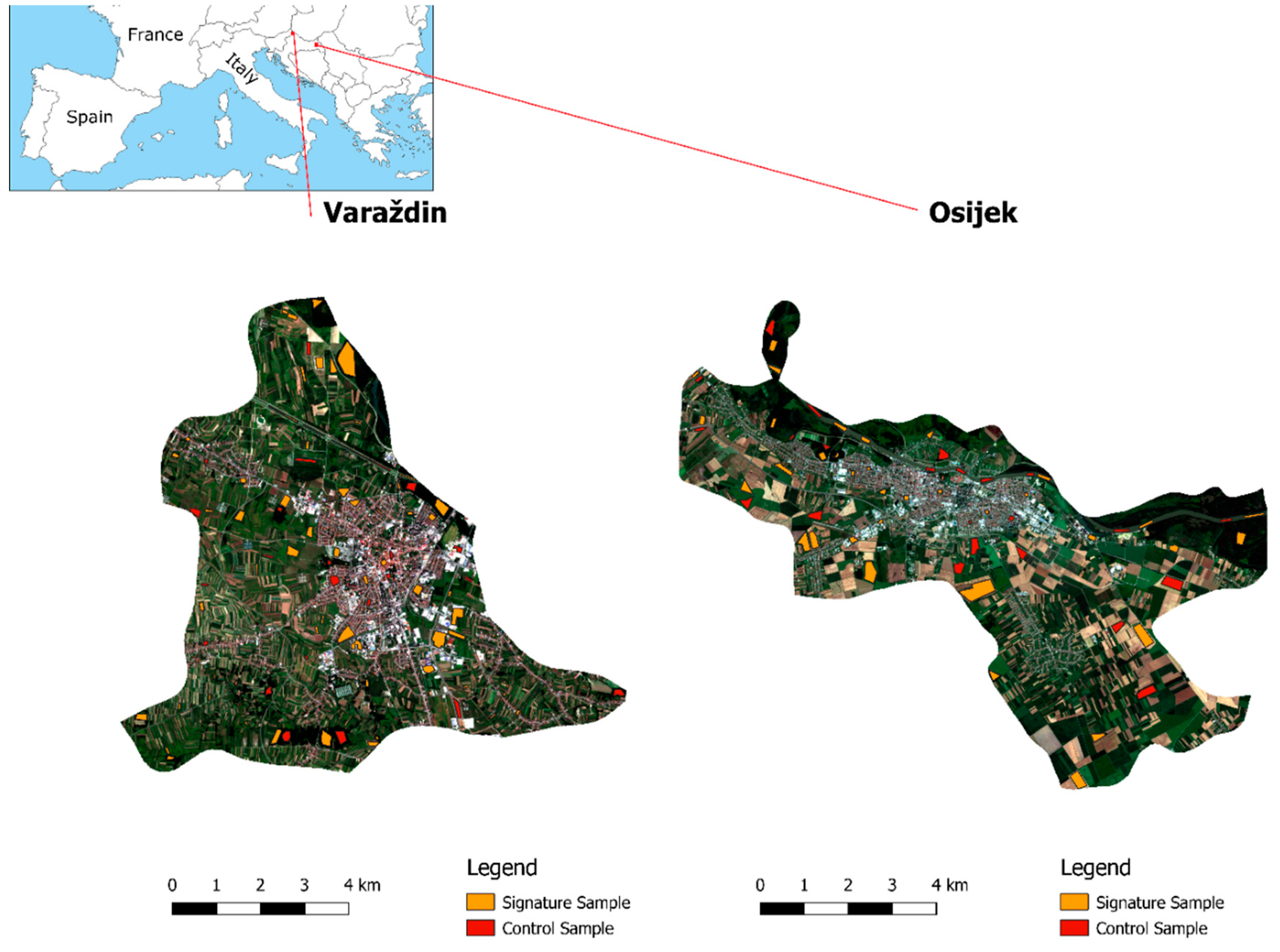
The study areas are located in two towns in Croatia: Varaždin and Osijek. The OpenStreetMap classification defines a town as an urban settlement with local importance and a population between 10,000 and 100,000. Both towns have a similar land cover use as they are located on the Drava River. The central area is populated with an urban fabric, and smaller areas are filled with green urban areas. The wider city center is populated with arable land, forests, and inland waters. The dominant types of vegetation in Varaždin are forests that are populated with beech, oak, and chestnut and large parks of grass and shrubbery [35]. The dominant types of vegetation in Osijek are grass and shrubbery; however, in Osijek, there are many swamp plants and linden and oak trees dominate the forest [36].

Table 3. The coordinates of the study areas (projection: EPSG 3765 | WGS84).

	E(m) | φ (d° m‘ s‘’)	N(m) | λ (d° m‘ s‘’)
Varaždin	487,550.00 | 46° 18’ 34.6’’	5,130,000.00 | 16° 20’ 18.1’’
Osijek	671,000.00 | 45° 33’ 03.3’’	5,048,000.00 | 18° 41’ 24.3’’

shows the coordinates of the center of the study area in Varaždin and Osijek. Figure 1 shows the study areas with a signature and control samples [15].

The first step was to download satellite images from the Copernicus Open Access Hub web page [31]. Since Sentinel-2A has a swath width of 290 km, it was necessary to crop the images to administrative areas of interest. That was done using diva-gis administrative data [37]. Afterwards, Dark Object Subtraction 1 (DOS1) atmospheric correction was performed on the imagery. DOS1 is a family of image-based corrections that have a lower accuracy than physical-based corrections; however, since DOS1 improves the estimation of land surface reflectance in satellite images, it was useful for this research [38]. The next step was to select signature samples and define parameters for the machine learning methods. The signature samples were selected using the red-green-blue (RGB) color composition and infrared (IR) channels since green urban areas are more visible on IR channels. For Varaždin, there were 69 signature and 26 control samples; for Osijek, there were 41 signature and 26 control samples. All image preprocessing was done using the QGIS and SAGA GIS software, and the accuracy assessment was performed in GRASS GIS and SAGA GIS. After the images were processed, we selected the parameters to be tested. The parameters were selected after a review of the literature and recommended combinations of parameters. The machine used is Intel ^® Core ™ i7-8550u, 16GB RAM, 64bit on Windows 10 operating system.

Table 4. The combinations of parameters for the artificial neural network.

	#1	#2	#3	#4	#5
Number of Layers	5	5	5	5	5
Number of Neurons	3	5	7	9	15
Number of Iterations	100	300	500	700	1500

presents five different combinations of parameters for the artificial neural network.

Table 5. The combinations of parameters for the random forest algorithm.

	#1	#2	#3	#4	#5
Maximum tree depth	5	10	20	30	50
Maximum sample count	1	2	4	6	10
Maximum number of categories	5	5	5	5	5

presents five different combinations of parameters for the random forest algorithm. Since the naïve Bayes algorithm is the simplest classifier, OpenCV does not provide the option to change the values of its parameters. We used the default values for parameters that are not mentioned. Parameters mentioned in Table 4 and Table 5 are numbered from 1 to 5 with # sign before them. In

Table 6. The accuracy assessment of the Artificial Neural Network for the Varaždin study area.

	#1			#2			#3			#4			#5
Class No.	C	O	est. Κ	C	O	est. Κ	C	O	est. Κ	C	O	est. Κ	C	O	est. Κ
1	NA	100.0	–999.0	NA	100.0	–999.0	NA	100.0	–999.0	NA	100.0	–999.0	NA	100.0	–999.0
2	0.06	1.40	0.99	3.57	0.45	0.94	62.65	0.00	0.00	33.56	0.00	0.46	16.37	0.00	0.74
3	44.33	9.78	0.50	59.14	12.97	0.34	NA	NA	NA	NA	NA	NA	26.92	96.21	0.70
4	NA	NA	NA	59.28	27.95	0.24	NA	NA	NA	NA	NA	NA	59.63	0.00	0.23
5	61.24	13.17	0.23	NA	NA	NA	NA	NA	NA	62.40	20.16	0.21	NA	NA	NA
Κ	0.521921			0.493735			0.000000			0.339945			0.435903

C, comission error; O, omission error; NA, not applicable.

,

Table 7. The accuracy assessment of the Artificial Neural Network for the Osijek study area.

	#1			#2			#3			#4			#5
Class No.	C	O	est. Κ	C	O	est. Κ	C	O	est. Κ	C	O	est. Κ	C	O	est. Κ
1	76.27	0.17	0.08	37.52	15.38	0.55	35.57	30.66	0.57	NA	100.0	–999.0	NA	100.0	–999.0
2	NA	NA	NA	0.00	42.91	1.00	NA	NA	NA	NA	NA	NA	NA	NA	NA
3	NA	NA	NA	38.30	23.28	0.46	56.17	23.28	0.21	60.54	0.00	0.15	59.38	1.37	0.17
4	8.94	1.62	0.88	8.01	5.54	0.89	17.51	0.65	0.76	8.39	3.61	0.89	14.89	0.79	0.80
5	NA	NA	NA	NA	NA	NA	NA	NA	NA	NA	NA	NA	NA	NA	NA
Κ	0.290510			0.676084			0.460587			0.362143			0.367605

C, comission error; O, omission error; NA, not applicable.

,

Table 8. The accuracy assessment of the random forest algorithm for the Varaždin study area.

	#1			#2			#3			#4			#5
Class No.	C	O	est. Κ	C	O	est. Κ	C	O	est. Κ	C	O	est. Κ	C	O	est. Κ
1	NA	100.0	–999.0	32.27	10.84	0.64	7.96	7.96	0.91	3.29	8.85	0.96	4.85	8.85	0.95
2	0.06	1.12	0.99	0.56	0.67	0.99	2.09	0.73	0.97	2.20	0.62	0.96	1.71	0.56	0.97
3	35.20	12.18	0.61	23.94	13.77	0.73	10.61	20.96	0.88	9.72	22.16	0.89	9.32	20.36	0.90
4	51.72	28.33	0.34	36.23	45.99	0.53	29.77	36.73	0.62	26.79	38.04	0.66	26.41	37.11	0.66
5	30.11	45.69	0.62	34.54	37.59	0.56	37.07	28.27	0.53	37.42	22.90	0.53	36.83	23.20	0.54
Κ	0.638237			0.726454			0.770248			0.778677			0.783603

C, comission error; O, omission error; NA, not applicable.

and

Table 9. The accuracy assessment of the random forest algorithm for the Osijek study area.

	#1			#2			#3			#4			#5
Class No.	C	O	est. Κ	C	O	est. Κ	C	O	est. Κ	C	O	est. Κ	C	O	est. Κ
1	45.17	17.46	0.46	33.59	25.97	0.59	2.77	27.01	0.97	2.79	26.64	0.97	5.10	23.25	0.94
2	0.00	10.12	1.00	0.02	3.09	0.99	0.02	0.49	0.99	0.02	0.25	0.99	0.02	0.32	0.99
3	15.15	41.34	0.79	5.89	26.96	0.92	2.43	3.88	0.97	2.25	4.13	0.97	0.56	7.46	0.99
4	10.13	1.45	0.86	20.42	2.19	0.72	14.09	2.75	0.81	15.19	3.16	0.79	13.80	3.02	0.81
5	97.63	97.46	-0.01	87.19	91.19	0.10	69.04	55.08	0.29	59.55	45.08	0.39	67.36	44.41	0.31
Κ	0.733440			0.676084			0.892828			0.895722			0.891797

C, comission error; O, omission error.

, results are presented in same manner, which means that the combination of parameters labeled #1 correspond to results labeled #1, and so on. Based on [39], where the author considered the number of trees and tree depth, we selected parameters for Table 5. The authors of [39] surmised that the larger the number of trees, the better the performance, but larger trees affect computational time, while deeper trees generally result in higher accuracy. However, if there is a need for faster results with less accuracy then less complex trees should be used. Therefore, in Table 5 for more complex trees there are more nodes and vice versa because this could show whether the less complex trees can achieve similar accuracy.

These parameters were used for both study areas. Table 6 shows the results of the accuracy assessment of the artificial neural network for Varaždin. Table 7 shows the results of the accuracy assessment of the artificial neural network for Osijek. Table 8 shows the results of the accuracy assessment of the random forest algorithm for Varaždin. Table 9 shows the results of the accuracy assessment of the random forest algorithm for Osijek.

Table 10. The accuracy assessment of the naïve Bayes algorithm for Varaždin (left) and for Osijek (right).

	Varaždin			Osijek
Class No.	C	O	est. Κ	C	O	est. Κ
1	45.97	0.66	0.49	43.71	9.29	0.47
2	0.06	1.06	0.99	0.00	0.60	1.00
3	42.53	10.18	0.53	5.35	41.32	0.93
4	50.0	44.10	0.36	16.19	40.98	0.78
5	0.00	77.81	1.00	94.41	77.63	0.03
Κ	0.642466			0.662983

C, comission error; O, omission error.

presents the results of the naïve Bayes classifier for Varaždin and Osijek.

In

Table 11. Execution time for each model for Varaždin (in seconds).

Parameter Combination.	SVM	ANN	NB	RF
#1	14.53	93.80	7.52	12.74
#2		91.14		13.78
#3		99.17		16.12
#4		130.24		17.14
#5		379.45		18.33

and

Table 12. Execution time for each model for Osijek (in seconds).

Parameter Combination.	SVM	ANN	NB	RF
#1	15.32	142.14	8.52	15.14
#2		97.42		15.98
#3		96.27		17.12
#4		113.41		17.44
#5		246.55		18.14

there is execution time for each model presented based on parameters defined in Table 4 and Table 5. Under column SVM (Support Vector Machine) and NB (naïve Bayes) there is only one record because for SVM is in this paper presented only the best combination of parameters from [15], while for NB there are no combination of parameter available as mentioned previously in text.

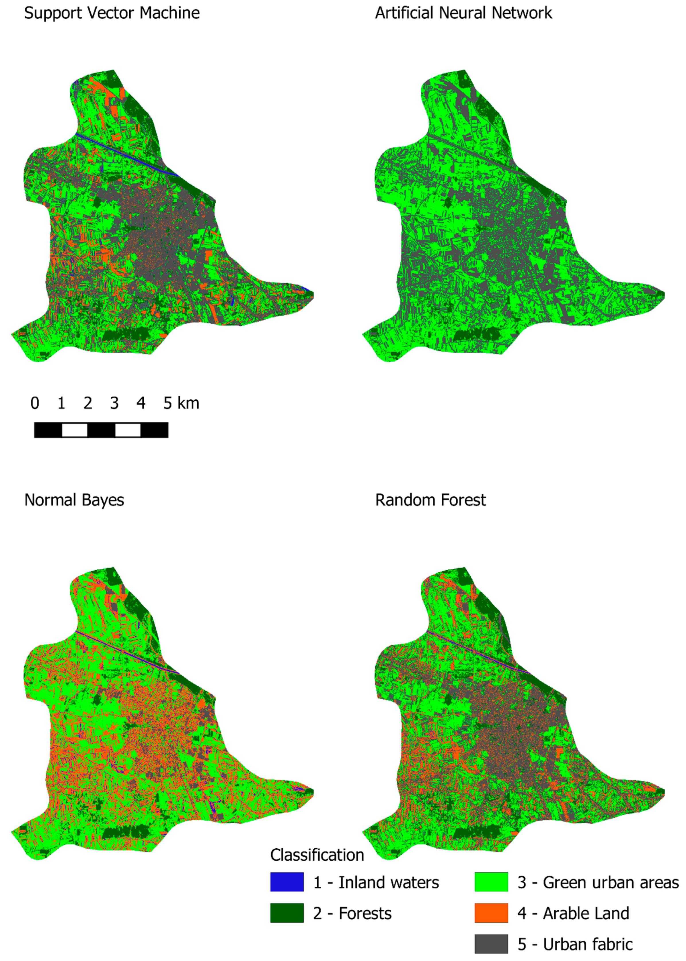
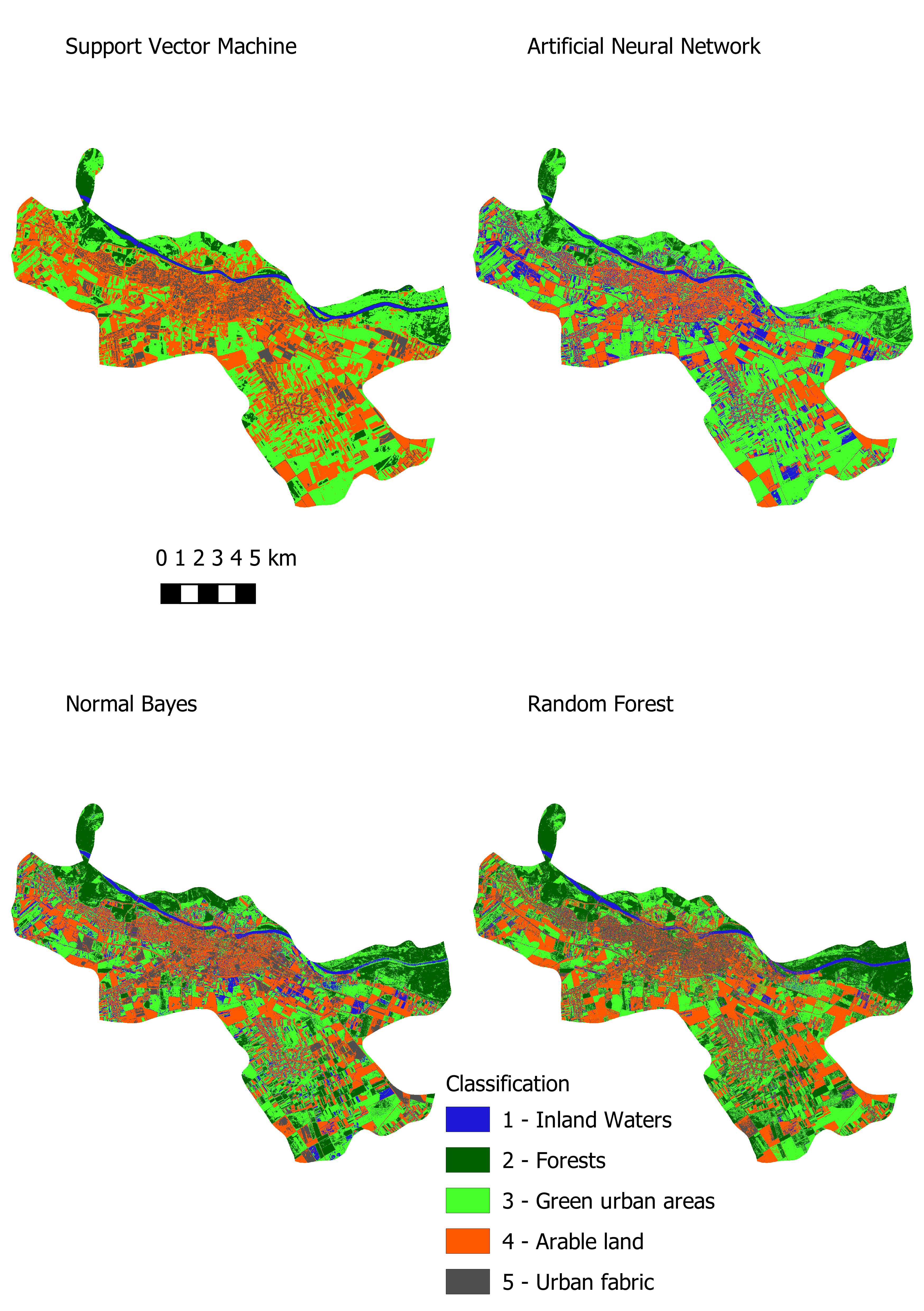
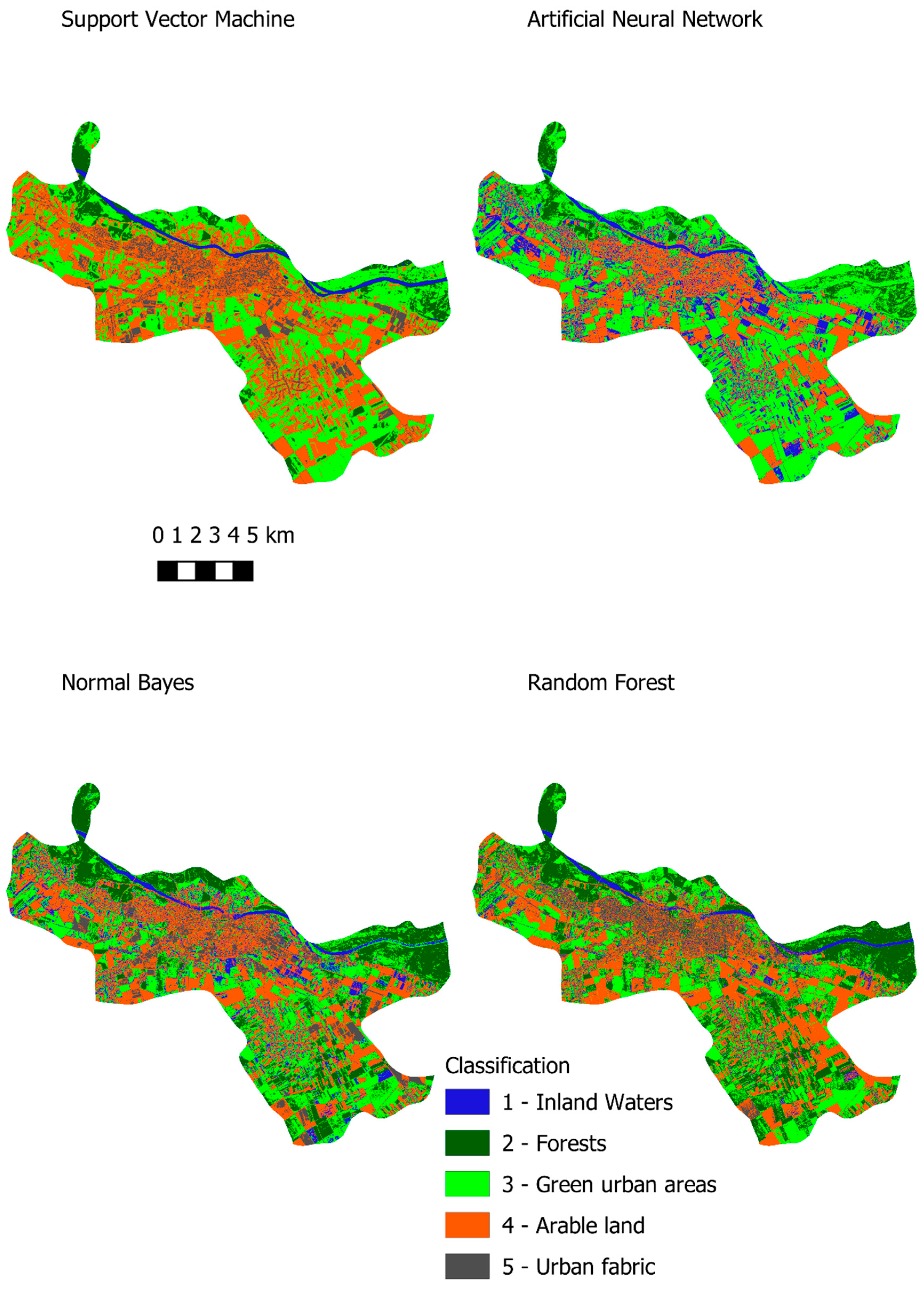
Figure 2 presents the results that provided the highest classification accuracy for each machine learning method for Varaždin. Figure 3 presents the results that provided the highest classification accuracy for each machine learning method for Osijek.

Regarding the Artificial Neural Network, the estimated kappa value is 0.52 for Varaždin and 0.67 for Osijek, which indicates a low classification accuracy. The Artificial Neural Network was also time-consuming which is shown in

Table 13. Overall performance with the best combination of each model for Varaždin.

	Support Vector Machine		Artificial Neural Network		Naïve Bayes		Random Forest
	Kernel	RBF	NL	5			MTD	50
	γ	1	NN	3			MSC	10
	C	28	NI	100			MNC	5
	Time	14.53	Time	93.80	Time	7.52	Time	18.33
Κ	0.867978		0.521921		0.642466		0.783603

RBF, radial basis function; NL, number of layers; NN, number of neurons; NI, number of iterations; MTD, maximum tree depth; MSC, maximum sample count; MNC, maximum number of categories; Κ, kappa.

and

Table 14. Overall performance with the best combination of each model for Osijek.

	Support Vector Machine		Artificial Neural Network		Naïve Bayes		Random Forest
	Kernel	RBF	NL	5			MTD	30
	γ	1	NN	5			MSC	6
	C	28	NI	300			MNC	5
	Time	15.32	Time	97.42	Time	8.52	Time	17.44
Κ	0.887217		0.676084		0.662983		0.895722

RBF, radial basis function; NL, number of layers; NN, number of neurons; NI, number of iterations; MTD, maximum tree depth; MSC, maximum sample count; MNC, maximum number of categories; Κ, kappa.

and compared to the other three machine learning methods, in this respect it is the poorest choice for the classification of green urban areas. Additionally, some of the classes were found to be unallocated or to have a low estimated kappa value; therefore, the artificial neural network is not recommended for the classification of green urban areas using Sentinel-2 imagery. The naïve Bayes algorithm is a good choice for classification when one needs to obtain information about a study area quickly and with high accuracy. The estimated kappa index is 0.64 for Varaždin and 0.66 for Osijek. If we focus on green urban infrastructure (class 3), the estimated kappa index is 0.53 for Varaždin and 0.93 for Osijek. This suggests that the results can vary in each class depending on the study area and that care should be taken when using the naïve Bayes algorithm to classify Sentinel 2 MSI imagery. Among other machine learning methods, naïve Bayes has the fastest execution time, which could be useful when one needs information quickly.

Random forest method provided high accuracy results. More complex trees with higher depth provided higher accuracy but with longer computation time, as expected. Smaller trees with fewer nodes performed well in a shorter time. This can be useful when results are needed faster than can be achieved while growing larger trees. When comparing the random forest algorithm with SVM, the following factors need to be taken into consideration: the estimated kappa for each class, the overall kappa, and the performance time. Performing a classification with SVM produced results on average 1.8 s faster than with the random forest algorithm, which could be significant when classifying larger areas. Regarding the SVM, the estimated kappa value for green urban infrastructure is 0.96 for Varaždin and the overall kappa value is 0.87. Regarding the random forest classifier, the estimated kappa value for green urban infrastructure is 0.89 for Varaždin and the overall kappa value is 0.78. From this, it is obvious that SVM outperformed the random forest classifier. However, different results were obtained for Osijek. For SVM, the estimated kappa value for green urban infrastructure is 0.89 and the overall kappa value is 0.89. For the random forest classifier, the estimated kappa value is 0.97 and the overall kappa value is 0.90. With respect to Osijek, the random forest classifier outperformed SVM.

Since SVM and Random forests have shown high accuracy and reasonable performance time, they could be considered for producing up to date maps of green urban areas in order to prevent green infrastructure in cities. Using machine learning methods can speed up map production and decision makers can have near real time data in order to decide which areas should be closely monitored in order to prevent further devastation. However, decision makers must be trained professionals who can supervise classification processes because sometimes, due to spectral similarity, urban fabric can be allocated in different classes. Therefore, although machine learning methods are getting more robust one should be careful when making decisions.

3. Conclusions

In this paper, analyses of four different machine learning methods was provided. Machine learning methods were tested on two different cities in Croatia. In general, support vector machine and random forest outperformed artificial neural network and naïve Bayes based on kappa statistics. Support vector machine and random forest had similar performance. However, for Varaždin and Osijek we recommend that the SVM machine learning method should be used for mapping green urban infrastructure as it produces results with high classification accuracy and is less time-consuming. Our next step will be to test our selected parameters and the SVM classifier on imagery from several different locations to obtain more results. For further research we will include K-nearest neighbor algorithm and try to optimize Artificial Neural Networks in order to achieve better results. Further research could develop a new machine learning method that can outperform SVM and the random forest algorithm at each location.