Abstract
Terrestrial laser scanning (TLS) technology has become increasingly popular in investigating displacement and deformation of natural and anthropogenic objects. Regardless of the accuracy of deformation identification, TLS provides remote comprehensive information about the measured object in a short time. These features of TLS were why TLS measurement was used for a static load test of an old, steel railway bridge. The results of the measurement using the Z + F Imager 5010 scanner and traditional surveying methods (for improved georeferencing) were compared to results of precise reflectorless tacheometry and precise levelling. The analyses involved various procedures for the determination of displacement from 3D data (black & white target analysis, point cloud analysis, and mesh surface analysis) and the need to pre-process the· 3D data was considered (georeferencing, automated filtering). The results demonstrate that TLS measurement can identify vertical displacement in line with the results of traditional measurements down to ±1 mm.
1. Introduction
Inspections of the condition of railway infrastructure and its relationship with railway traffic commenced in the mid-19th century after the Dee Bridge disaster in Chester, forming the basis for the first engineering safety standards for structures [1]. In the 1950s, the operational railway speed was below 100 km·h−1. Modern freight trains reach 160 km·h−1, while passenger trains reach 350 km·h−1 [2]. It is necessary to ensure compatibility of the engineering capabilities of trains with the operational capabilities of the railway infrastructure, which is often old. This need arises from the European trend to develop high-speed rail. Over 40% of railway bridge infrastructure in Poland has reached the upper limit of its design life. As these structures were usually designed for loads lower than the actual operational loads, they undergo accelerated structural degradation, which results from fatigue [3]. Railway companies in Western Europe have been continuously emphasising the necessity of inspections aimed at verifying their load-bearing capacity in the new environment of high-speed railway since the 1990s [2].
The terrestrial laser scanner is an active remote sensing system for determining coordinates (X, Y, Z) and the intensity of reflected beam (I) for points representing the surface of an object. One of the first promising laboratory studies on the implementation of TLS in displacement and deformation measurements demonstrated that, with favourable environmental conditions, TLS measurement can be used to measure the vertical displacement down to ±0.29 mm [4]. The application of TLS in displacement and deformation measurement has been widely investigated regarding both geometry [5,6] and spectral analyses of the intensity of the reflected beam [7,8]. The papers have been partially, extensively summarised and organised by researchers from the University of Nottingham Ningbo [9]. The application of quick, remote, and comprehensive measurement technology itself does not guarantee satisfactory results of displacement and deformation measurements. In addition to the class and type of the terrestrial laser scanner and the measurement method, the method of post-processing TLS data is just as important. Precise registration, filtration, and modelling of 3D data are necessary in order to obtain TLS data of satisfactory precision and reliability for the purpose of determining structural displacement. The processes involved in post-processing of TLS measurement results should be selected in such a way as to match the geometry and type of structure with a particular focus on the quality of 3D data of those components of the structure that reflect the structural mechanics directly.
The specific character of laser scanning of elongated objects, the span of bridge structures, and their location over an obstacle affect the measurement method [10]. The linear nature of the structure makes it impossible to apply cloud to cloud registration. To obtain at least a 30% overlap of consecutive scenes would require excessive concentration of scanner positions or would be entirely impossible in the case of opposite positions. 3D data in a terrestrial laser scanning of bridge structures should be interconnected via an appropriate, planned external network of control (reference) points with as many interrelations as possible. Civil engineering structure stability testing should employ such TLS data registration that facilitates control over the process. Not only does the registration of point clouds using artificial reference objects that are uniquely identifiable in the scanned space ensure control over transformations [11] (verification of geometric relationships between points of a 3D model and in the georeference system) but it also facilitates obtaining a resultant point cloud with a satisfactory value of the mean registration error. Control point coordinates determined using traditional methods with a high enough accuracy that make up the base for the registration of data from individual scanning positions reduce transformation errors and ensure TLS data amplification [12].
The definition of TLS reliability according to the theory of calculus of error as a derivative of the probability of gross errors is unjustified. This is because terrestrial laser scanning noise has to be removed from model space, preferably using filtration algorithms. The reliability of laser scanning, can, therefore, be defined as the measure of the effectiveness of the filtration process [13] necessary to optimise in-field observations and further analyses of 3D data. Measurement noise, which is the primary cause of systematic modelling errors and contributing to the increased measurement uncertainty [14], depends to a large extent on the characteristics of the scanned scene. Hence, measurement noises should be subjected to dedicated filtration algorithms [15]. The primary features facilitating the classification of points as measurement noise by filtration algorithms are the range of object occurrence, satisfied neighbourhood condition, and the intensity of the reflected beam. According to the literature, 3D object datasets should be cleaned at the stage of raw scanning results and further analyses should be free of their influence [15].
One popular solution used in testing civil structure stability using TLS is to generate surface models from point clouds and compare them at regular intervals. The primary argument for the creation of surface models of objects is that terrestrial laser scanners never measure the same element of the structure twice. Therefore, a generalisation of a point cloud into a surface model is a better representation of the periodic condition of the structure due to its homogeneity [16]. Moreover, according to a commonly recognised classification [17], cloud models represented by point clouds are treated in some applications as low-detail models of 3D objects [18]. Opponents of point cloud generalisation, on the other hand, believe surface models as derivatives of point clouds do not represent the actual condition of a structure and a significant part of spatial information is lost as a result of the generalisation. Delaunay triangulation is the basis for the generation of surface models in 2D, 2.5D, and 3D space both for TIN and TEN (tetrahedral networks) [18,19]. The use of the Delaunay algorithm with Voronoi diagram does away with the issue of ambiguous results of tessellation of the set of elements of a point cloud [20]. The diversity of algorithms for generating surface models based on Delaunay triangulation (recursive split, divide and conquer, step by step, incremental, incremental delete and build, radial sweep, Pitteway triangulation, hierarchical [21]) results from research published over decades [20]. The abundance of approaches to building surface triangle networks corresponds to the great number of software applications for automated model generation available on the market. The use of the most automated modelling for shapes that are sufficiently discrete builds a representation of structural elements made up of triangulated irregular network triangles. The primary drawback of this solution is very time-consuming triangulation [18]. It is not always true that the higher the density of a point cloud, the better the local approximation of the plane, even in displacement measurement [16]. Oversampling leads to poor surface model quality where local fitted triangular planes join each other at sharp angles, which leads to coarseness and discontinuities in the model. It is, therefore, justified to adhere to a popular TLS guideline that the optimum scanner resolution should be at least equal to the error of the measurement of the scanner-to-object distance [16].
The comprehensive results, cost of technology, and the remote nature of the measurements would make terrestrial laser scanning a good solution for the assessment of the stability of bridge structures during static load testing. Perhaps that is why Lichti et al. [22] were among the first researchers who used TLS to capture vertical deflections of a bridge that was subjected to a static load condition up to 65.75 tons. The 3D analysis procedure was aimed at generating a mesh surface model of no-load and load TLS data of the object and to extract cross-sections. Deflections were estimated from the vertical displacement between epoch cross-sections at both the top and bottom of each section. Displacements measured from the top of the cross-sections were burdened with an RMS error of ±4.9 mm. Subsequently, Zogg and Ingensand [23] used TLS to monitor deformations of the Felsenau viaduct bridge during a static load test. They captured point clouds of several sections of the object before and after loading and then compared them to each other in the Geomagic Qualify software. The point cloud differentiation results differed from precise levelling ones by less than ±3.5 mm, with a mean residual less than ±1.0 mm.
Hungarian scientists analysed the application of TLS to compute deformation of the bridge structure under load as well [24]. For epoch TLS data, they compared mesh surface models (in the Geomagic 8 software) and used measurements of point clouds (in cross-sections). The authors concluded that the structural displacements determined using laser scanning datasets were strongly correlated with those obtained from traditional techniques. The first ones cannot, however, be evaluated at the same accuracy level as traditional high-precision equipment.
Application of TLS technology for bridge load tests has also been investigated by Mill et al. [25]. The procedure of post-processing TLS data included removing noise from point clouds, creating surface meshes, and analysing deformation on the basis of a surface created from the TLS data before the load test and surfaces from TLS data collected during a static load test. The results of the 3D analysis were compared to those from precise levelling. The differences between terrestrial laser scanning and precise levelling vary within a few millimetres. The research showed a ±2.8 mm accuracy of terrestrial laser scanning at a 95% confidence level.
Lõhmus et al. [26] conducted a similar determination of vertical displacements of two bridges during static load tests. In addition to comparing epoch mesh surfaces of point clouds and their compatibility with precise levelling, tacheometry, and dial gauge results, the authors described in detail point cloud modelling and the deformation determination procedures. The research showed that TLS analyses can detect changes of the structure with an accuracy of up to ±1 mm. The studies also showed examples of a lower accuracy of TLS technology in this respect. The authors also pointed out that the TLS provides a complete set of 3D spatial information on bridge structure deformations, which may be far more important than achieving the maximum accuracy.
An attempt to define a method for testing the stability of elongated structures using TLS should focus on the determination of whether a specific quantity of collected spatial data for an object can reliably identify structural changes during static load testing after preprocessing. The paper describes the determination of the displacement values for girders of an old steel railway bridge during static load testing using TLS and precise traditional methods. The study used methods of point cloud post-processing and displacement determination using TLS data from the cited papers. The results of the study were also compared with traditional land surveying methods. However, the authors made an objective assessment of the usefulness of providing georeferencing, preparing the object for measurement, or operations on point clouds. The analyses of 3D data involved various procedures for the determination of displacement (black & white target analysis, point cloud analysis, and mesh surface analysis) and the need to pre-process the 3D data were considered (georeference, automated filtering).
2. Materials and Methods
2.1. Tested Bridge
The bridge static load test took place at a steel railway bridge of railway line No. 098 (Figure 1). It is located in the south of Poland, on the 2.485th kilometre of the railway line that is a part of the railway route that connects Krakow and Zakopane. The bridge was built in the 1960s as part of a route upgrade project aimed at increasing the vertical alignment of the track over the Skawa River. The legal basis for the project was Engineering Norm D-64 1956.

Figure 1.
Tested bridge on railway line No. 098.
The structure of the railway bridge is a double-span continuous suprastructure with effective design span of 52.700 m + 52.700 m = 105.400 m. The structure is supported on concrete angled abutments and a support. The bridge centre line intersects with the obstacle at 55°. The total width of the railway bridge is 5.400 m. The structure has a single, 4.500 m track. The maximum total load is 6980 kg·cm−2. The calculated deflection of the bridge caused by the static weight of the structure is 1.820 cm; the deflection caused by a moving load is 3.700 cm; and the maximum movement rating is ±3.200 cm.
The design and operation documentation demonstrated discontinuities in structure condition tests. The only diagnostics operation on the bridge over many years of operation was periodic visual inspections to assess the general condition of the object. In theory, the static parameters of the over 50-year old infrastructure element continue to apply despite the railway revolution in the recent decades that redefined the conditions for the use of railway infrastructure.
The stability of the old steel structure has been researched since 2014 in cooperation with the Polish railway infrastructure company PKP PLK S.A. The research focuses on the application of remote measurement technologies to determine the periodic displacement of the structure. Before the research, control network points and controlled network points had to be designed and mounted. The results of the stability tests of the control network points and controlled network points were used during the static load test of the railway bridge as well.
2.2. Bridge Static Load Testing
The static load tests of multi-span railway bridges in Poland are often performed for single bridge spans as per commonly used loading models [27]. Local loading of complex structures helps determine the dynamics of changes in structures that are unevenly loaded directly during and after the loading. The representative spans for measurement are usually selected by the railway administrator [28]. In the present research, the static load test was performed for the span for which a complete point cloud could be registered.
After the structure was measured in the unloaded state directly before the static load test, the span was loaded with a passenger rolling stock EN57 (Figure 2). The loaded bridge span was immediately below the motor wagon of the total service weight of 126.5 t. The exact location of the test loading diagram was obtained after consultation with a railway line diagnostics technician.
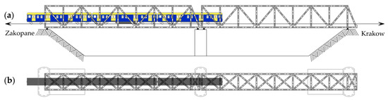
Figure 2.
Static loading diagram for the bridge span; (a) lateral view; (b) bird-eye view.
During the movement of the load, vehicle-structure vibrations occurred, which would cause irreversible distortions in results had they not been damped. In order to avoid the impact of the disturbance on the results, the measurement was interrupted until the effect of the vibration was negligible. The structural vibration damping was verified as per PN-S-10050:1989. The displacement of specific points of the loaded span was measured directly after the load was applied and every 15 min. When the increase in displacement over the recent quarter did not exceed 2% of the measured value, the final value was considered robust. Otherwise, the loading remained unchanged until the increase in the deflection was less than the 2% [29]. After 60 min of loading, test measurements of bridge deflection through periodic readout of the height change on an invar rod indicated that the vibrations were damped to a satisfactory degree.
2.3. Survey and TLS Measurements
The concept for the measurement involved three methods of determination of the displacement during the static load test of the bridge. The first one was precise levelling, the second was precise reflectorless tacheometry of a controlled point network (black and white—B&E targets fixed to the structure of the bridge), and the third one was terrestrial laser scanning of the railway bridge. Each measurement variant was performed twice, directly before the loading and during the static load test. Each of the three methods of determining the stability of the railway bridge was capable of measuring displacement. Bridge span levelling and tacheometric measurement of controlled points had an additional function. They provided reference values for values obtained with TLS.
Precise levelling was performed from two measuring positions, over an abutment and over the bridge support (Figure 3a). The levelling involved 18 structural protrusions of girders (marked as 10P–18P, 10L–18L on Figure 3b). They were vertically aligned with the points of the controlled network (Figure 3b,c). The precise levelling was carried out using the Leica NA3003 digital level and the Leica GPCL2 invar staff. Due to the small size of the observation sample, adjustment was carried out assuming the constancy of the average unit error (Mo = 1). The accuracy of observation (significance) in adjustment was measured with the value of the standard deviation for the height difference per 1 levelling station (0.40 mm). This a priori accuracy of measurement was equal to twice the value of the accuracy of a set of measuring instruments.
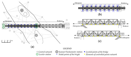
Figure 3.
Measurement conditions; (a) situation; (b) levelled points on the bridge span; (c) the elements of controlled points network measured using tacheometry.
Reflectorless tacheometry measurements of the points in the controlled network and terrestrial laser scanning were performed in the same real time alternately on the same measuring positions (Figure 3a). During the measurement, levelling heads with adapters were levelled and centred once. Depending on the solution needed, adapters of the heads were fitted with retroreflectors or reference targets. Reflectorless tacheometry measurements of 36 points of the controlled network were carried out using a Trimble VX (angular accuracy 1ʺ, EDM accuracy 1.0 mm + 2.0 ppm Prism/2.0 mm + 2.0 DR) and in three measuring series.
The object was scanned using a phase-based laser scanner Z+F 5010. The operations performed at the scanning position [30] involved a preliminary low-resolution measurement aimed at defining the scan site. Next, the scanner was tied to the reference targets located over the points of the control network. After the position was referenced, proper scanning of the railway bridge was commenced (resolution of 40,000 points/360°) and selected B&W targets of the controlled network were rescanned. The situational and vertical compatibility of point clouds with levelling and tacheometry results was ensured by a two-step tie-in procedure. The first step was to tie scanning positions to points of the control network. Points of horizontal control helped with precise horizontal referencing of TLS data. The height of reference targets was determined roughly down to 1.0 mm with trigonometric levelling. The literature on the determination of the height of point clouds using reference targets indicates less reliable results than for situational referencing of spatial data using such targets [31]. A vertical laser beam entails greater representation deformations in the vertical plane than in the horizontal plane. In order to improve the vertical reliability of the point cloud, an additional solution was applied, reference spheres. White reference spheres placed at set intervals in the measured space were levelled precisely (Table 1). The heights of the centres of the reference spheres were determined in the control network. Levelled centres of the reference spheres represented centres of gravity of spheres modelled in the 3D space of the scanner. White reference spheres (75 mm radius) were precisely extruded. Measurement of the roundness in the cross-section of the spheres by the radial method showed deviation from sphericity of 0.2 mm. The deviation from sphericity represented the accuracy of the radius. The heights of the centres of the reference spheres were equal to the heights of the tops of the spheres minus the radius.

Table 1.
Point cloud registration steps.
2.4. TLS Data Processing
Point cloud analyses resulted directly from the assumed procedure to determine the optimal post-processing of TLS data. The procedure involved the determination of object displacement using three different methodological approaches implemented for datasets to which different preprocessing was applied (Table 2). Results of the changes in the object during the static load test from 3D analyses were compared to results of reflectorless tacheometry and precise levelling so that the variant of 3D processing most compatible with traditional measurements could be identified.
Table 2.
Procedures of post-processing of TLS data.
The point clouds were registered in two stages (Table 1). Each stage required traditional surveying measurements in order to improve the quality of TLS data. Data were registered in Leica Cyclone 9.2.0.
The periodic point clouds of the railway bridge were filtered using the following algorithms: SOR filter, Noise filter, and bilateral filter. These filters use three different approaches to reduce measurement noise. The SOR filter first calculates the mean distance of each point to K closest neighbouring elements and then removes those points that are further from their neighbours than the maximum distance equal to the sum of the calculated mean distance and its multiple standard deviations nSigma, as below:
Configuration parameters used in the study were:
and the number of points used for mean distance estimation was 6.
The Noise filter uses Euclidean distances between cloud points and local base planes it fits around every point in the dataset. For 3D data, the Noise filter is an example of a low-pass filter. The following parameters were used for filtration using the Noise filter: neighbours - points (kNN) was 6, the maximum absolute error was 1. Additionally, the function Remove isolated points was used. The bilateral filter is a non-linear image detection algorithm, which preserves object edges, reduces noise, and smooths geometries. It is implemented for post-processing of point clouds and their products. The bilateral filter analyses the return beam intensity and replaces it with a weighted average of intensities of neighbouring units. The bilateral filter was applied with two parameters: spatial sigma (the Normal distribution variance for the spatial part of the filter) and scalar sigma (the Normal distribution variance for the scalar part of the filter). The spatial sigma was 0.020 and the scalar sigma was 1022. All configuration parameters of all filters were determined empirically. The filtration algorithms were run in CloudCompare 2.6.1., which is compatible with PCL (Point Cloud Library) tools.
Surface models of lower beams of the girder were generated using Geomagic Wrap 12. The advanced features of the spatial data processing algorithms based mainly on the least square method ensure the high metrological quality of resulting data distinguished with a Special Quality Certificate of the National Institute of Standards and Technology (NIST) [33]. Surface models were generated using the Wrap function and the default method of smoothing was Prismatic Shapes Conservative, which preserves such details as sharp edges. According to [34] the Wrap function produces shapes and surfaces by taking subcomplexes of the Delaunay complex of the data set S. Let a, b, c, and d be four points in S then abcd is a tetrahedron in the Delaunay complex if and only if all other points lie outside the unique sphere that passes through a, b, c, and d. The set of tetrahedra together with their triangles, edges, and vertices make up the Delaunay complex. Wrap uses an incremental algorithm for constructing the complex and symbolic perturbation to reduce any degenerate configuration to the genetic case. The Wrap function is dimension-independent and it is able to automatically and freely mix different dimensions as required by the data set. After using the Wrap function, the Prismatic Shapes Conservative was used in one iteration. The Prismatic Shapes Conservative method is dedicated to mechanical compound shapes. During triangulation, it aims at matching subsets of point clouds to regular geometric figures (spheres, half-spheres, cuboids, cones). This method does not eliminate measuring noise at the edges to maintain the desired shape.
Spatial displacement values of B&W targets in procedure (1) were determined based on coordinates of centres of the B&W targets approximated in Leica Cyclone 9.2.0. The measures of reliability, RMS (mean registration error) and (mean error of fitting the object in a point cloud of a regular object) affected the value of the vector of error of the identified displacement directly.
Differential models of point clouds (procedure (2)) were obtained in CloudCompare 2.6.1 with an algorithm based on the neighbourhood principle (nearest neighbour distance). Differential models of surface triangle networks (procedure (3)) were generated in Geomagic Control 2015 using a directional algorithm with vector . The maximum distance (0.032 m, the maximum calculated deflection of the bridge) was taken into account when generating the differential models (procedures (2) and (3)). Values above this threshold were considered as identified incorrectly. The accuracy of calculated vertical translocations of girder beams was analysed using a solution proposed by researchers from the Tallinn University of Technology [25].
The conformity of displacement values calculated on the basis of the B&W target analysis and the traditional method was verified with a statistic for comparing feature distribution in two samples. The Kolmogorov–Smirnov (K-S) test for two samples is widely used in civil engineering. It is a good statistic for determining the consistency of displacement because it is sensitive not only to differences in distribution location but also their shapes. The applied version of the compliance test facilitated comparison of the distributions of two samples of random variables with a sample size smaller than in the case of a parametric Student t-test. The significance level (α) for the statistic was 1%. The cluster analyses of the first and the second sample were performed with the cluster size equal to the accuracy of TLS registration (1 mm), (in accordance with the principle that the size of a cluster should not be greater than the unit used for a given scale problem) [35]. To verify the compatibility of displacement, the authors verified:
Null hypothesis:
H0:
vs.F1(TLS) = F2(TACH): The empirical distribution functions of the first and the second sample respectively are identical.
Alternative hypothesis:
Ha:
F1(TLS) ≠ F2(TACH): The empirical distribution functions of the first and the second sample respectively are not identical.
For results of procedures (2) and (3), parameters for assessing the displacement difference accuracy were calculated () for every single node of the girder (), determined using laser scanning () and precision levelling ():
The parameters for assessing the accuracy of differences in displacement values included standard deviation (s), median absolute deviation (D), maximum absolute deviation (), average absolute deviation ():
Chi-Square test of significance for the variance was used for values . According to value , the sample of differences in displacement values should not exhibit variance greater than mm2. The variance of values of procedures (2) and (3) was verified in terms of meeting criterion , assuming that the distribution of samples of is normal. The authors verified:
Null hypothesis:
H0:
vs. = : The differences are not statistically significant.
Alternative hypothesis:
Ha:
> : The differences are statistically significant.
The significance level (α) for the statistic was 1%.
3. Results and Discussion
Results of the adjustment of the epoch precision levelling of bridge spans during the static load test demonstrated high accuracy and almost 50% relevant reliability of the measurements. The average mean height error in adjusted values was 0.4 mm. Results of adjustment of tacheometric measurements demonstrated the average error of location of a controlled point of 1.0 mm (situation) and 0.7 mm (height).
The two-stage registration of point clouds resulted in 3D material with registration accuracy up to 0.001 m (MAE) (Table 3). MAE (Mean Absolute Error) facilitates the evaluation of the accuracy of the entire registration process between the base coordinate system and coordinate systems of point clouds. In structural stability studies, a registration accuracy of 1 mm is the absolute criterion for TLS to be useful in displacement and deformation analysis [26]. The two-step registration of point clouds facilitated uninterrupted control over the process through verification of the relationship between consecutive scanning positions. Additionally, cloud height adjustment improved the quality of vertical TLS data, which is usually lower than the horizontal data quality. As a result of the filtration of point clouds, the size of spatial datasets was reduced by almost 11%. The only difference between the resulting surface models for the two variants of point clouds (automatically filtered and unfiltered) was the coarseness of the model. The applied default surface model generation method dedicated to complex mechanical shapes was aimed at fitting subsets of cloud points into regular geometric shapes (spheres, hemispheres, cuboids, or cones). No noise on edges was removed during the process of building a regular network of triangles. The desired shape was therefore retained.
Table 3.
Results of TLS data registration; Point cloud of the bridge after registration, (a) Before static loading; (b) Before static loading – cross-section; (c) During static loading – cross-section; (d) During static loading.
3.1. B&W Target Analysis (1)
The investigation into the bridge stability during test static load based on TLS data in line with procedure (1) demonstrated a qualified mobility of 57% of elements of the loaded bridge span. The criteria of the accuracy of resultant mean errors of components of displacement was mm, mm, and mm. An analysis of the consistency of displacement distributions determined using TLS and traditional surveying methods carried out with the use of the K-S test for two samples (Table 4) supported a conclusion that the two analysed samples had a common population. According to the plots of distribution functions of random variables (Figure 4), the best consistency was noted for vertical displacement, which is of vital importance in structural stability testing under a static load.
Table 4.
K-S test results for displacement samples, TLS vs. TACH.
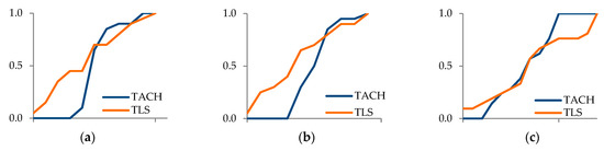
Figure 4.
Spatial displacement distribution functions of two independent samples TACH vs. TLS; (a) along the OX axis, (b) along the OY axis, (c) vertical.
Tests of stability of the railway bridge based on the spatial displacement of points determined based on georeferenced point clouds demonstrated statistical consistency with results of reflectorless tacheometry. The indicated method for determining spatial displacement does not contribute to the improvement of the observations apart from the rightness of the statement that reflectorless tacheometric survey gives results close to the fitting of the elements into the point cloud of a reference target. The quality of analysed point clouds may be a consequence of georeferencing of the system of coordinates, which requires design, mounting, and periodic verification of stability of the control network. The monitoring of the displacement of B&W targets implies the necessity to prepare the investigated object. The investigation into the railway bridge stability during the static load test and using B&W target analysis satisfies the accuracy criterion for reflectorless measurements but fails to satisfy the conditions of quick, remote measurement. The demonstrated consistency of displacement of points can, however, justify analyses of displacement of the object under static load using the obtained 3D data (analyses in procedure (2) and (3)).
3.2. Point Cloud Analysis (2)
Vertical displacement values of the beam loaded in procedure (2) were determined for three sets of 3D data using different preprocessing procedures. The result was differential models of point clouds without sophisticated post-processing (set(A)) (Figure 5a), differential models of georeferenced point clouds (set(B)) (Figure 5b), and differential models of georeferenced and algorithm-filtered point clouds (set (C)) (Figure 5c). The resultant value of the mean error of vertical displacement determined a priori for TLS measurements according to [25] was ±2.4 mm (confidence level of 95%).
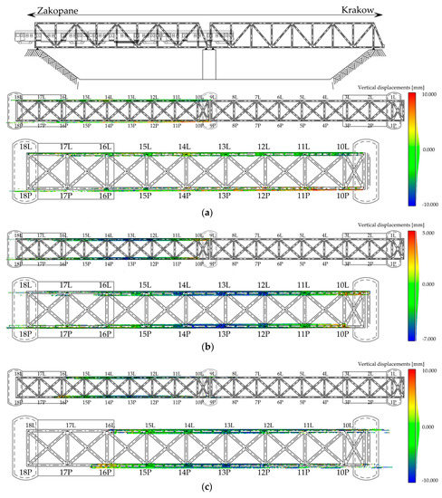
Figure 5.
Results of point cloud analysis (2); (a) set (A) of TLS data, (b) set (B) of TLS data, (c) set (C) of TLS data.
In order to verify the consistency of the determined displacement with results of precise levelling for each structural node of the girder, a representative group of 30 indicators of point displacement was approximated. The typical displacement value in the group was determined, which reflected the largest percentage of vertical translocation values in the sample. The three approximated sets of displacement values were compared to results of precise levelling (Figure 6) by calculating differences in displacement values and their parameters for assessing accuracy that were the measure of dispersion (Table 5).
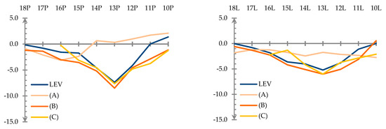
Figure 6.
Displacement values from point cloud analysis (2) and precise levelling (LEV) [mm].
Table 5.
Point cloud analysis (2) results.
The methodology of testing the railway bridge stability that involved a differentiation of 3D datasets from TLS measurements indicated that point clouds referenced to an external surveying control (set (B)) facilitate the determination of vertical displacement values that are the closest to the values determined using precise levelling (Table 5). The large number of observations, which is typical of 3D data, in the differentiation of raw point clouds is not indicative of a reduction of the mean error of displacement values compared to traditional methods. Neither do filtration algorithms that improve the reliability of spatial data ensure better consistency of displacement values determined using TLS with results of traditional methods in comparative analyses of point clouds. Still, filtration significantly reduces systematic errors (value ) (Table 5). The results of the analysis of the parameters for assessing the accuracy of differences in displacement values were confirmed by Chi-Square test results for differences in displacement values (Table 6).
Table 6.
Significance for the variance test results of differences in displacement values .
The potential of point cloud differentiation in testing displacement and deformation was appreciated by investigators examining the condition of the Felsenau viaduct. They believed differential models of point clouds were capable of identifying vertical displacement within the mm-range [23]. Point cloud analysis (2) confirms these results. Apart from the degree of compliance of TLS and precision levelling, however, they indicate the importance of not only automatic filtration but also georeferencing. Similar conclusions about accuracy were offered in an article by researchers from the University of North Carolina. Although they did not focus on the importance of procedures of TLS data capturing and post-processing, they emphasised the importance and user-friendliness of working with TLS data in projects to detect damage in railway infrastructure [36]. Note that this concept of determining structural mechanics and its consequences has certain drawbacks. First of all, its sensitivity to minor deformations is limited [37,38]. In order to obtain reliable results of displacement, one needs to use point clouds with as large a density as possible because this feature will ensure identification of not only relatively minor dislocations but also any possible systematic errors during differentiation [39].
3.3. Mesh Surface Analysis (3)
Mesh surface analyses (3) conducted for sets (B) and (C) of input data demonstrated displacement values for a continuous girder structure of 5 mm to almost –15 mm (Figure 7). The consistency of structural nodes (Figure 6), approximated as in the case of point cloud analysis (2), with the reference was discussed.
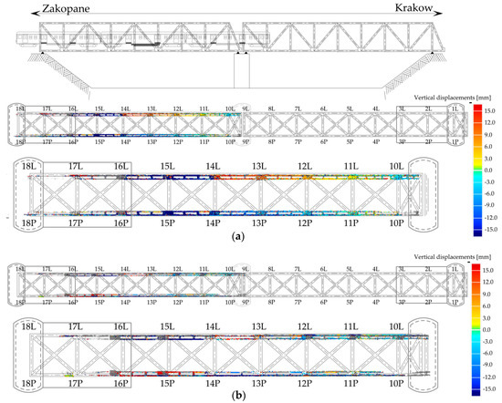
Figure 7.
Results of mesh surface analysis (3); (a) set (B) of TLS data, (b) set (C) of TLS data.
Analysis of two sets of spatial data after different preprocessing indicated a greater consistency with reference values of surface models that were generated from georeferenced point clouds subjected to automated filtering (Table 7). The differentiation of surface models generated from unfiltered point clouds (B) completely failed to reflect the structural mechanics during static loading (Figure 8, Table 7). The a priori assumed mean error of determination of vertical displacement from TLS data () was significantly reduced in analyses of set (C). It was indispensable to filter point clouds for mesh surface analyses in order to ensure a ±1.3 mm consistency of the determined displacement values with the reference. The differentiation of surface models from generalised point clouds did not identify any vertical displacement for marginal structural protrusions of the girders. Surface models are recommended for high-resolution numerical data subjected to automated filtering, which improves the reliability and thus helps eliminate systematic errors almost completely without a risk of removal of structural data during the clean-up. For mesh surface analysis (3), the results of the analysis of the parameters for assessing the accuracy of differences in displacement values were confirmed by Chi-Square test results for differences in displacement values (Table 8).
Table 7.
Mesh surface analysis (3) results.
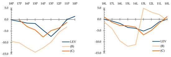
Figure 8.
Plot of displacement values from mesh surface analysis (3) and precise levelling (LEV) [mm].
Table 8.
Significance for the variance test results of differences in displacement values .
Mesh surface analyses (3) were used to determine displacement in bridge stability tests in Estonia: The Loobu highway bridge and the Tartu railway overpass. Researchers from the Tallinn University of Technology demonstrated that TLS and differentiation of mesh surfaces can identify vertical displacement during static load tests with the standard deviation of ±0.8 mm to ±3.4 mm in relation to precise levelling results [26]. The millimetre accuracy of vertical displacement (by mesh surfaces analysis (3)) has been confirmed in this study. In addition, Lõhmus et al. formulated an assumption that the accuracy of TLS is mainly the result of the capability and peculiarities of the TLS technology. Their importance (e.g. measurement noise or data post-processing) has been parameterized in this study. Surface models of point clouds are an adequate solution for surface objects such as cooling towers [40], dams [41,42], or tunnels [43]. The comparison of periodic surface models of an object in order to detect dislocation is a recognised procedure in landslide monitoring [44,45] and determining the progress of erosion of rocky cliffs [46,47,48]. The investigation into displacement and deformation of natural objects does not, however, require as great an accuracy as work with civil structures.
4. Conclusions
The TLS measurement during the static load test of the railway bridge and different post-processing procedures led to the following general conclusions.
- The registration of point clouds in stages with vertical adjustments of TLS data provided scan data, the accuracy of which is high enough to identify vertical displacement of structural elements with the same accuracy as in the case of reflectorless measurements.
- The accuracy of the determination of the centre of B&W targets based on a high-resolution point cloud is similar to the accuracy of reflectorless tacheometry (carried out in several repeats with two positions of the telescope).
- The determination of structural displacement based on differential models from raw point clouds after gross manual filtration is an unreliable method that fails to identify periodic dislocations of the same values and sign as traditional methods. The reason for the failed determinations is the application of cloud to cloud registration for differentiation. This type of registration matches point clouds using the least square method and minimises the Euclidean distance between them, thus removing periodic displacement.
- The large number of observations, which is typical of 3D data, in the differentiation of raw point clouds does not result in a reduction of the mean error of displacement values compared to traditional methods.
- Georeferencing of the external coordinate system of point clouds – determined with high relative reliability and using precise traditional methods – reduces the assumed resultant mean error of displacement by half during the differentiation of the point clouds.
- By improving the reliability of spatial data, filtration algorithms eliminate systematic errors almost completely.
- Generalisation and homogenisation of point clouds (after georeferencing only) with algorithms for generating surface models do not facilitate a reliable determination of displacement.
- Surface models are recommended only for high-resolution numerical data subjected to filtering algorithms.
- The use of surface models for investigating object stability is justified only for point clouds, the density of which is around 2 mm. In the case of less favourable resolutions, numerical data are lost when generating surface models and in the process of filtering and generating surface models.
- The maximum value of the displacement during the static load test (−7.4 mm) was lower than the maximum design deflection (−18.2 mm). A detailed inspection of the railway bridge, which was carried out with the participation of a railway diagnostician before and after the trial load, did not find any irregularities in the structure of the tested object.
The TLS measurement during the static load test of the railway bridge facilitates identification of displacement with an accuracy of ± 1 mm regardless of the post-processing method but is still behind precise surveying methods. TLS measurement should be used as an auxiliary tool to supplement traditional precision levelling.
Author Contributions
All authors contributed significantly to the manuscript. P.G. was responsible for the original idea, collected the data, conducted data analysis, and contributed to manuscript revision. M.M. contributed to field data collection and provided theoretical and conceptual inputs.
Funding
This research was partly financed by the Ministry of Science and Higher Education of the Republic of Poland (4361/KG/2015, 2306/KG/2018) and is a part of the PhD thesis of the first Author.
Conflicts of Interest
The authors declare no conflict of interest.
References
- Taylor, W.M. Iron, Engineering and Architectural History in Crisis: Following the Case of the River Dee Bridge Disaster, 1847. Archit. Hist. 2013, 1, 23. [Google Scholar]
- Klasztorny, M. Dynamika mostów belkowych obciążonych pociągami szybkobieżnymi (en. Dynamics of Beam Bridges Loaded with High-Speed Trains); Wydawnictwa Naukowo-Techniczne: Warszawa, Poland, 2005. [Google Scholar]
- Kużawa, M.J.; Cruz, P.J.S.; Bień, J. Analysis and fatigue evaluation of Pinhao bridge in Portugal. Mosty stalowe: Projektowanie, technologie budowy, badania, utrzymanie. In Proceedings of the Tytuł ten podsumowuje konferencję, Wroclaw, Poland, 27–28 November 2008. [Google Scholar]
- Gordon, S.; Lichti, D. Modeling Terrestrial Laser Scanner Data for Precise Structural Deformation Measurement. J. Surv. Eng. 2007, 133, 72–80. [Google Scholar] [CrossRef]
- Georgopoulos, G.D.; Telioni, E.C.; Tsontzou, A. The contribution of laser scanning technology in the estimation of ancient Greek monuments’ deformations. Surv. Rev. 2018, 48, 303–308. [Google Scholar] [CrossRef]
- Xu, X.; Bureick, J.; Yang, H.; Neumann, I. TLS-based composite structure deformation analysis validated with laser tracker. Comp. Struct. 2018, 202, 60–65. [Google Scholar] [CrossRef]
- Cho, S.; Park, S.; Cha, G.; Oh, T. Development of Image Processing for Crack Detection on Concrete Structures through Terrestrial Laser Scanning Associated with the Octree Structure. Appl. Sci. 2018, 8, 2373. [Google Scholar] [CrossRef]
- Wujanz, D.; Burger, M.; Tschirschwitz, F.; Nietzschmann, T.; Neitzel, F.; Kersten, T.P. Determination of Intensity-Based Stochastic Models for Terrestrial Laser Scanners Utilising 3D-Point Clouds. Sensors 2018, 18, 2187. [Google Scholar] [CrossRef] [PubMed]
- Mukupa, W.; Roberts, G.W.; Hancock, C.M.; Al-Manasir, K. A review of the use of terrestrial laser scanning application for change detection and deformation monitoring of structures. Surv. Rev. 2017, 49, 99–116. [Google Scholar] [CrossRef]
- Kędzierski, M.; Fryśkowska, A.; Wilińska, M. Naziemny skaning laserowy obiektów inżynieryjno—Drogowych (en. Terrestrial laser scanning of engineering and road objects). Biuletyn WAT 2007, 59, 285–308. [Google Scholar]
- Gosliga, R.; Lindenbergh, R.; Pfeifer, N. Deformation analysis of a bored tunnel by means of Terrestrial Laser Scanning. ISPRS 2006, 36, 5. [Google Scholar]
- Leica Geosystems. Leica Cyclone 7.2 Tutorial, Part: Registration. 2007. Available online: https://arf.berkeley.edu/files/webfiles/all/arf/equipment/field/3d_scanner/cyrax_leica_laser/Cyclone/Cyclone%205.8.pdf (accessed on 10 November 2018).
- Toś, C.; Wolski, B.; Zielina, L. Zastosowanie tachimetru skanującego w praktyce geodezyjnej (en. Application of the total station in surveying practice). Środowisko. Czasopismo techniczne 2010, 16, 1–17. [Google Scholar]
- Lichti, D.D.; Gordon, S.J.; Tipdecho, T. Error models and propagation in directly georeferenced terrestrial laser scanner networks. J. Surv. Eng. 2005, 131, 135–142. [Google Scholar] [CrossRef]
- Weinmann, M.; Jutzi, B. Geometric point quality assessment for the automated, markerless and robust registration of unordered TLS point clouds. ISPRS Ann. Photogramm. Remote Sens. Spat. Inf. Sci. 2015, II-3/W5, 89–96. [Google Scholar] [CrossRef]
- Van Genechten, B.; Schueremans, L. Laserscanning for heritage documentation. Wiadomości konserwatorskie 2009, 26, 727–737. [Google Scholar]
- Foley, J.D.; Van Dam, A.; Feiner, S.K.; Hughes, J.F.; Philips, R.L. Wprowadzenie do grafiki komputerowej (en. Introduction to Computer Graphics); Wydawnictwa Naukowo-Techniczne: Warszawa, Poland, 2001. [Google Scholar]
- Pyka, K.; Mikrut, S.; Moskal, A.; Pastucha, E.; Tokarczyk, R. Problemy automatycznego modelowania i teksturowania obiektów opisujących skrajnię linii kolejowych (en. Problems of automatic modeling and texturing of objects describing objects of railway lines). Archiwum Fotogrametrii, Kartografii i Teledetekcji 2013, 25, 177–188. [Google Scholar]
- Quintero, M.S.; Genechten, B.; Bruyne, M.; Poelman, R.; Hankar, M.; Barnes, S.; Caner, H.; Craven, P.; Budei, L.; Heine, E.; et al. 3D RiskMapping. Theory and Practice on Terrestrial Laser Scanning. Training Material Based on Practicial Applications; Universidad Politécnica de Valencia: València, Spain, 2008. [Google Scholar]
- Izdebski, W. Wykłady z systemów informacji o terenie (en. Lectures on land information systems); Politechnika Warszawska: Warszawa, Poland, 2015. [Google Scholar]
- Mitka, B.; Piech, I. Modele powierzchni terenu (en. Surface models). Infrastruktura i Ekologia terenów wiejskich 2012, 3, 167–180. [Google Scholar]
- Lichti, D.D.; Gordon, S.J.; Stewart, M.P.; Franke, J.; Tsakiri, M. Comparison of digital photogrammetry and laser scanning. Int. Soc. Photogram. Remote Sens. 2008, 39–44. Available online: https://www.researchgate.net/profile/Jochen_Franke3/publication/245716767_Comparison_of_Digital_Photogrammetry_and_Laser_Scanning/links/541ba09d0cf25ebee98d98f3/Comparison-of-Digital-Photogrammetry-and-Laser-Scanning.pdf (accessed on 5 November 2018).
- Zogg, H.M.; Ingensand, H. Terrestrial laser scanning for deformation monitoring—Load tests on the Felsenau Viaduct (ch). Int. Arch. Photogram. Remote Sens. Spat. Inf. Sci. 2008, 37, 555–562. [Google Scholar]
- Lovas, T.; Barsi, A.; Detrekoi, A.; Dunai, L.; Csak, Z.; Polgar, A.; Berenyi, A.; Kibedy, Z.; Szocs, K. Terrestrial laser scanning in deformation measurements of structures. Int. Arch. Photogram. Remote Sens. Spat. Inf. Sci. 2008, 37, 527–532. [Google Scholar]
- Mill, T.; Ellmann, A.; Kisa, M.; Idnurm, J.; Idnurm, S.; Horemuz, M.; Aavik, A. Geodetic monitoring of bridge deformations occurring during static load testing. Baltic J. Road Bridge Eng. 2015, 10, 17–27. [Google Scholar] [CrossRef]
- Lõhmus, H.; Ellmann, A.; Märdla, S.; Idnurm, S. Terrestrial laser scanning for the monitoring of bridge load tests—Two case studies. Surv. Rev. 2018, 50, 270–284. [Google Scholar] [CrossRef]
- Łaziński, P.; Pradelok, S. Badanie odbiorcze wieloprzęsłowego wiaduktu kolejowego nasuwanego poprzecznie (en. Acceptance test of multi-span railway over-slip rail); Wrocławskie dni mostowe. Obiekty mostowe w infrastrukturze miejskiej: Wrocław, Poland, 2013. [Google Scholar]
- Chróścielewski, J.; Malinowski, M.; Miśkiewicz, M. Próbne obciążenia mostu przez Wisłę w Puławach (en. Load tests of the bridge over the Vistula River in Puławy); Wrocławskie dni mostowe. Mosty stalowe. Projektowanie, technologie budowy, badania, utrzymanie: Wrocław, Poland, 2008. [Google Scholar]
- The Polish Committee for Standardization (Polski Komitet Normalizacyjny—PKN). PN-S-10050:1989 Obiekty mostowe—Konstrukcje stalowe—Wymagania i badania. (en. Bridge structures—Steel constructions—Requirements and tests.); Polski Komitet Normalizacyjny—PKN: Warszawa, Poland, 1989. [Google Scholar]
- Mitka, B. Możliwości zastosowania naziemnych skanerów laserowych w procesie dokumentacji i modelowania obiektów zabytkowych (en. Possibilities of using terrestrial laser scanners in the process of documentation and modeling of historic buildings). Archiwum Fotogrametrii i Teledetekcji 2007, 17, 525–534. [Google Scholar]
- Boehler, W.; Marbs, A. Investigating Laser Scanner Accuracy. 2003. Available online: www.leica-geosystems.com (accessed on 4 November 2018).
- Gawronek, P. Methodology of Determining Stability of Bridges Using Terrestrial Laser Scanning. Ph.D. Thesis, Faculty of Environmental Engineering and Land Surveying, University of Agriculture in Krakow, Kraków, Poland, 2017. (In Polish). [Google Scholar]
- United States Department of Commerce. Report of a Special Test. NIST Test No. 681/280055-10. 2010. Available online: https://3dssupport.microsoftcrmportals.com/66d243af5d014342b9de97b5c8cac2e (accessed on 2 November 2018).
- Edelsbrunner, H.; Facello, M.A.; Fu, P.; Qian, J.; Nekhayev, D.V. Wrapping 3D Scanning Data. In Proceedings of the Photonics West ‘98 Electronic Imaging, San Jose, CA, USA, 6 March 1998. [Google Scholar]
- Plucińska, A.; Pluciński, E. Probabilistyka (en. Probability); Wydawnictwo Naukowo-Techniczne: Warszawa, Poland, 2000. [Google Scholar]
- Shen-En, C. Laser Scanning Technology for Bridge Monitoring. In Laser Scanner Technology; InTech: London, UK, 2012; ISBN 978-953-51-0280-9. [Google Scholar]
- Bitelli, G.; Dubbini, M.; Zanutta, A. Terrestrial laser scanning and digital photogrammetry techniques to monitor landslides bodies. Int. Arch. Photogram. Remote Sens. Spat. Inf. Sci. 2004, 3, 246–251. [Google Scholar]
- Schäfer, T.; Weber, T.; Kyrinovic, P.; Zámecniková, M. Deformation measurement using terrestrial laser scanning at the hydropower station of Gabcikovo. In Proceedings of the INGEO 2004 and FIG Regional Central and Eastern European Conference on Engineering Surveying, Bratislava, Slovakia, 11–13 November 2004. [Google Scholar]
- Tsakiri, M.; Lichti, D.D.; Pfeifer, N. Terrestrial laser scanning for deformation monitoring. In Proceedings of the 3rd IAG/12th FIG Symposium, Baden, Austria, 22–24 May 2006. [Google Scholar]
- Ioannidis, C.; Valani, A.; Georgopoulos, A.; Tsiligiris, E. 3D Model Generation for Deformation Analysis Using Laser Scanning Data of a Cooling Tower. In Proceedings of the 12th FIG Symposium, Baden, Austria, 22–24 May 2006. [Google Scholar]
- Alba, M.; Fregonese, L.; Prandi, F.; Scaioni, M.; Valgoi, P. Structural monitoring of a large dam by terrestrial laser scanning. Int. Arch. Photogram. Remote Sens. Spat. Inf. Sci. 2006, 36, 6. [Google Scholar]
- Oliveira, A.; Oliveira, J.F.; Pereira, J.M.; De Araújo, B.R.; Boavida, J. 3D modelling of laser scanned and photogrammetric data for digital documentation: The Mosteiro da Batalha case study. J. Real-Time Image Process. 2014, 9, 673–688. [Google Scholar] [CrossRef]
- Delaloye, D. Development of a New Methodology for Measuring Deformation in Tunnels and Shafts with Terrestrial Laser Scanning (LIDAR) Using Elliptical Fitting Algorithms. Master’s Thesis, Queen’s University, Kingston, ON, Canada, 2012. [Google Scholar]
- Monserrat, O.; Crosetto, M. Deformation measurement using terrestrial laser scanning data and least squares 3D surface matching. ISPRS J. Photogram. Remote Sens. 2008, 63, 142–154. [Google Scholar] [CrossRef]
- Kim, M.K.; Kim, S.; Sohn, H.G.; Kim, N.; Park, J.S. A New Recursive Filtering Method of Terrestrial Laser Scanning Data to Preserve Ground Surface Information in Steep-Slope Areas. ISPRS Int. J. Geo-Inf. 2017, 6, 359. [Google Scholar] [CrossRef]
- Rosser, N.J.; Petley, D.N.; Lim, M.; Dunning, S.A.; Allison, R.J. Terrestrial laser scanning for monitoring the process of hard rock coastal cliff erosion. Q. J. Eng. Geol. Hydrogeol. 2005, 38, 363–375. [Google Scholar] [CrossRef]
- Barbarella, M.; Di Benedetto, A.; Fiani, M.; Guida, D.; Lugli, A. Use of DEMs Derived from TLS and HRSI Data for Landslide Feature Recognition. ISPRS Int. J. Geo-Inf. 2018, 7, 160. [Google Scholar] [CrossRef]
- Shen, Y.; Wang, J.; Lindenbergh, R.; Hofland, B.; Ferreira, V.G. Range Image Technique for Change Analysis of Rock Slopes Using Dense Point Cloud Data. Remote Sens. 2018, 10, 1792. [Google Scholar] [CrossRef]


© 2019 by the authors. Licensee MDPI, Basel, Switzerland. This article is an open access article distributed under the terms and conditions of the Creative Commons Attribution (CC BY) license (http://creativecommons.org/licenses/by/4.0/).