Exploiting the Potential of Integrated Public Building Data: Energy Performance Assessment of the Building Stock in a Case Study in Northern Italy

Abstract

Smart management of urban built environment relies on the availability of data supporting sound policy making and guiding city renovation processes toward more sustainable and performant models. Nevertheless, public managers are unlikely to have comprehensive information on the existing building stock. In addition, tools providing effective insights on potential costs and benefits of retrofit strategies at city/district scale are hardly available. This article describes how data related to existing buildings may be effectively combined together into a so-called Building Information System, and discusses the advantages and shortcomings related to this process. At the same time, the implementation on a real case study in northern Italy demonstrates how the effort due to data harmonization and integration is able to foster applications to support policy makers in the management of the built environment and in the definition of urban sustainability strategies. Building data were harmonized according to the requirements of the international open standard CityGML, therefore facilitating the exchange of building information. The whole project was carried out while considering the characteristics of data sources that are available for each public body in Italy and, as a consequence, it may be replicated to other Italian municipalities.

1. Introduction

The increased attention paid to the anthropogenic impacts on natural environment has raised awareness on the themes of efficiency, sustainability, and resilience of urban settlements. Contemporary buildings are expected to be very performant from many points of view, ensuring a better quality and a lower carbon footprint of the built environment [1], a higher protection and resilience from catastrophic events [2], and a smarter management of assets [3]. If, on one side, nowadays, it is easy to obtain complete information on new or recent buildings, on the other hand it may not be so easy to retrieve the same quality and quantity of data regarding older, existing buildings. However, the current building stock accounts for the largest part of European cities and entire portions of settlements require a systemic transformation and renovation strategies in order to meet higher sustainability and efficiency requirements. Conversely, the city-wide availability of proper informative tools on urban objects (e.g., buildings, bridges, etc.) to guide such strategies is not always ensured.

The quality and completeness of building information in Italy is characterized by several criticalities: building data are often incomplete and out of date; contents are often replicated in different databases but information may differ due to the different rate they are updated; and, data are not correlated as neither semantic nor spatial references are shared among existing archives [4]. In short, building information is spread among heterogeneous sectorial databases, each one created for a specific purpose and following an application-oriented approach in data modelling, organization, and management. Consequently, data collection and harmonisation tasks still represent a barrier for the adoption of proper tools supporting policy makers in the definition of urban development and renovation strategies [5].

The need for organized and usable information on buildings is an issue that has been addressed for some decades by several European countries. In the Netherlands, for example, the creation of an integrated set of key public registers started at the beginning of ‘90s [6,7]. Such registers, which are considered to be of primary importance for the public sector, include both geographic data (cadastre, small and large-scale topographic base maps, addresses, buildings, subsoil utility networks) and non-geographic data (residents, companies, vehicles, etc.). The scope of this harmonization process was to improve the management efficiency, the update frequency and the usability of public archives. Consequently, a better reliability of the public informative heritage was achieved, so that this became a real service provided by the cadastre to local businesses [8]. This also eased the creation of a National Spatial Data Infrastructure (NSDI), enabling in recent years the creation of three-dimensional (3D) city models nationwide [9]. In Germany, at the beginning of the 2000s, cadastre and topographic information were recognised as the most important base information for GIS. Increasing demands from the market (real estate agencies, banks, insurance companies, etc.) encouraged public authorities to set up an integrated data model for cadastre and topographic database: the contents of the two archives were defined in order to avoid redundancies and duplicated data acquisition, and to enable data interchange [10]. The availability of harmonised building data also facilitated the creation of 3D city models. In the UK, the national mapping agency (Ordnance Survey) is in charge of the continuous update and maintenance of core geographic information (GI), which may be used by public bodies and private companies as reliable and certified data. Among others, it also includes building-related information. Ordnance Survey is also partner in a pilot project coordinated by the Open Geospatial Consortium (OGC) and buildingSMART International, focusing on the integration of 3D city models and building models. The mapping agency is also involved in the Digital Built Britain, a government initiative aimed to solicit the digitalisation process within the construction sector [11,12]. In Spain, the national cadastre aimed to go beyond its purely fiscal purpose and moved to the 3D mapping of buildings, which includes the modelling of building interiors and distinguishes floors and building units [13,14].

The lesson learnt by these experiences may be summarised, as follows:

• GI plays a significant role in the modelling of building data, especially when considering that built assets are influenced by the context in which they are located (e.g., the definition of cadastral revenue is influenced by the central or peripheral location within a city) and, in turn, they may influence that context (e.g., construction of a new building shading other buildings and increasing the heating energy demand during the winter season);
• the existence of harmonized archives is the key for the provision of complete information on buildings, integrating structural and constructive details (e.g., number of floors and dwellings, physical properties of the construction materials), and socio-economics data (e.g., number of residents, presence of companies and elderly people, etc.); and,
• shared and federated data management mechanisms may improve the efficiency in public data handling, avoiding redundancies and incoherencies, and improving the rate of data updating.

The objective of the research presented in this article was to create an integrated Building Information System (BIS) starting from the available information on buildings, which is supposed to enable archive interoperability and provide a complete picture of the building stock within a city. The aim is to demonstrate how such efficiency plans and strategies may be implemented at the district and city scale.

To this purpose, a review of the available building data sets in public archives was made, highlighting their pros and cons and identifying a feasible way to link them (Section 2.1). Further on, a case study area in Italy was selected, where significant harmonisation work was carried out in order to create the BIS and to bridge the gap between expected and actual data quality. 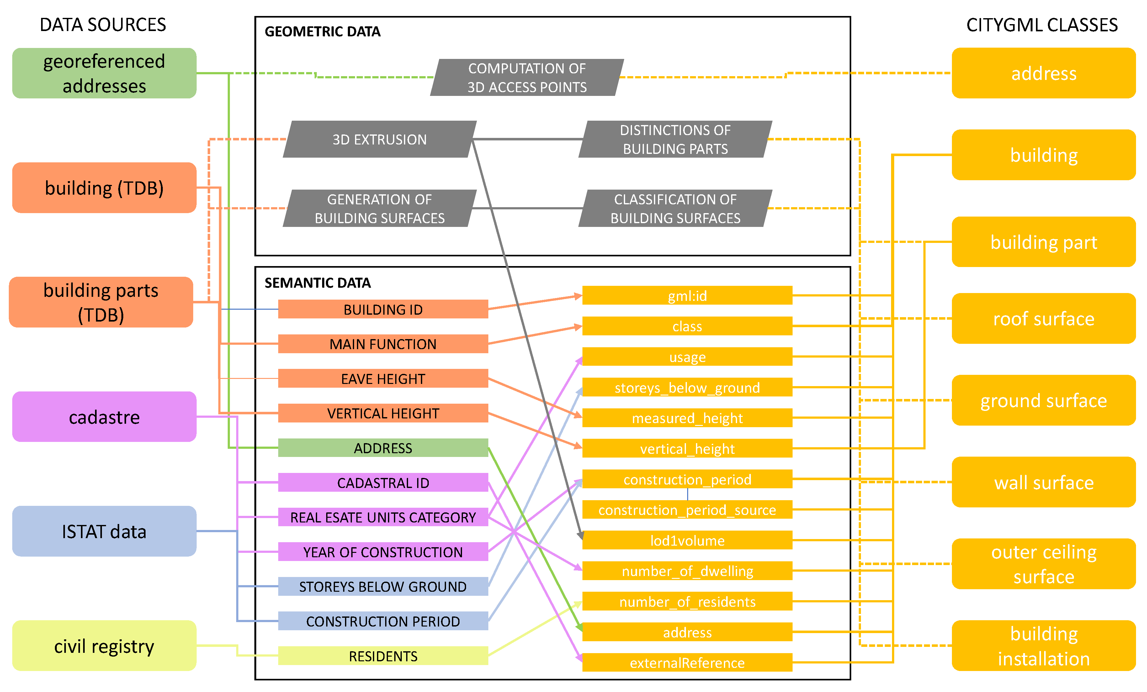Integrated data were then combined and modelled according to the international standard CityGML (Section 2.2). In addition to the “base” data model, building data were also structured following the Energy Application Domain Extension (ADE), which extends the base model and provides a common reference for building energy simulation. Finally, a practical case study concerning the estimation of the primary energy demand for winter heating at district scale was accomplished (Section 2.3): the estimated values were then compared with energy performance certificates (EPC) and measured consumption values, allowing for evaluating the accuracy of energy analysis carried out on a set of 154 residential buildings (Section 3). It has to be highlighted that the point of view assumed in this research is the one of a public body: all public authorities in Italy have indeed a privileged access to building data and can use them for public, collective purposes.

This article is mainly derived from and it further extends the Ph.D. dissertation of one of the authors [15], which deals with building data integration. However, this article intentionally focuses on the practical use cases related to building and energy modelling, as well as building analyses at district scale, in order to demonstrate how the effort required to foster data interoperability may lead to an effective usability of public data in urban analyses and applications. A comprehensive description concerning all open issues that are related to public building data or about the practical operations to enforce data interoperability is however beyond of the scope of this article and can be found in the abovementioned document.

2. Materials and Methods

2.1. Creation of the Building Information System

2.1.1. Building data

The main scope of this research was to identify a viable way for the Italian local administrations to create a BIS starting from available data. Bearing in mind this objective, building data sources were identified by considering those databases that could be accessed by every municipality within a standardized approach. As a consequence, this entailed the exclusion of some interesting data sets that were managed at regional level (e.g., databases of energy performance certificates or thermal plants), whose availability, informative contents, and acquisition procedure may differ from one region to another. Thus, a review of the available data sources was carried out and the following archives were selected to be included in the BIS:

• Topographic Database (TDB): as the current official format for local and regional topographic maps, TDB has a 2.5D, object-oriented data structure, which is aimed to provide a geometric and semantic description of real-world objects [16]. The coordinate reference system used in Italian TDB refers to the European Terrestrial Reference System ETRS 89, projected according to UTM (zones 32 and 33 North). The data model for TDBs is compliant with those requirements defined by the European Directive 2007/2/EC INSPIRE [17]. Each object is represented through self-consistent geometry associated to attributes describing its main features; objects relate one to each other on the basis of topologic and consistency constraints. As far as built assets are concerned, buildings in TDBs are defined as set of volumes (roughly corresponding to CityGML building parts) composing a unique built object: this building has a specific architectonical typology (e.g., generic building, skyscraper, church, warehouse, etc.), a prevalent usage (one of: residential, public services, industrial), and a level of maintenance (one of: under construction, in use, disused, or ruined). Thus, for every building mapped in a TDB, it is possible to compute its 3D geometry by processing geometric data stored as building parts, and to know few generic features (e.g., typology and main function). As purely cartographic products obtained through stereoplotting from aerial imagery, contents that are related to non-visible parts, such as underground floors, or details related to vertical surfaces (e.g., openings), are not reported. Other data sources (e.g., cadastre, BIM models) should be queried to retrieve this missing information items. However, the integration with other external data sources phase is not required by current technical specifications, disregarding the possibility to set up a continuous informative flow from existing administrative procedures (e.g., data input coming from construction permit procedures);
• Cadastre: the Land Registry is the only database on buildings that is formally available all over the country. Cadastral identifiers are the only official references for the identification of a building in Italy, uniquely identifying every single asset nationwide. Nevertheless, its contents have a merely fiscal nature and updates are produced only for new or refurbished buildings. The basic unit censed in the Land Registry is the Real Estate Unit (REU, in Italian: Unità Immobiliare Urbana). According to national legislations this is a portion of building (e.g., a dwelling within a block of flats), a whole building (e.g., a house), or a group of buildings (complex constructions such as hospitals or industrial settlements) that, given its state, may independently produce an income [18]. As far as the building characteristics are concerned, two types of information are of interest, given the scope of this work: (1) the cadastral map, allowing for a spatial localization of parcels, buildings, roads and water bodies; and, (2) the REU descriptive information, providing fine-grain data on qualitative and quantitative parameters related to each real estate. Cadastral updates are submitted by construction professionals on behalf of property owners. However, optional requirements are often disregarded given the difficulty to gather precise information on older buildings. Moreover, no automatic procedures are set to assess the completeness and consistency of such updates;
• ISTAT microdata: every ten years the Italian National Institute of Statistics (ISTAT) collects up-to-date information to describe the consistency of the national building stock. A part of this survey overlaps those data gathered by the cadastral procedure in the case of registration of new buildings or after refurbishment of old ones. Differently from cadastral updates, data are extensively collected for all the existing buildings. Thus, the lack within the cadastral information could be overcome by information coming from census data. Despite this chance, no common references are explicitly defined in the two databases to this purpose. The main reference is the address: thus, it is the only piece of GI that may enable the geocoding of building data. Fortunately, addresses that are associated to buildings censed by ISTAT are reported in a structured way and aligned with the national archives of addresses. This should ensure an automatic connection between ISTAT microdata and georeferenced addresses normally available in local administrations; and
• Energy consumption data: electricity and gas consumption data are reported for every Point-of-Delivery (POD) registered in energy providers’ databases. A single POD may refer to a single or many households: it is currently not possible to determine which properties are connected to a specific POD as cadastral references are omitted from this database. What is known is that all PODs linked to the same address serve the building associated to that address. As in the case of census data, the address is the only reference that is usable to link buildings to PODs, but unlike census data, addresses are reported in an unstructured way and are sometimes incomplete. Consequently, the automatic linking to georeferenced addresses is not ensured and it is often difficult to associate consumption values to the correct building in the real world. Data available for each utility connection are: POD number, fiscal code of the energy provider, client’s fiscal code, address associated to the connection, type of connection (i.e., residential or non-residential), amount of energy consumed (expressed as kWh/year of electricity and as m³/year of gas), and consumption bills (in Euros).

A summary of building data sources is reported in

Table 1. Summary of building data considered.

Data Source	Characteristics	Criticalities
Topographic Database (TDB)	georeferenced, object-oriented data model; semantic and geometric building data city-wide; compliant with international standards;	production still in progress; no connection with other external data sources;
Cadastre	main reference for building data comprising fine grain information on real estates; comprises geographic reference;	updates available only for new or renovated real estates; no automatic procedure to check the quality of data provided by professionals;
Census data	shared contents with cadastral archives; extensive update of building data every 10 years;	address as building key identifier; no geographic reference;
Energy consumption data	fine-grain electricity and gas consumption data for every Point of Delivery (POD) within a municipality; possibility to analyse energy consumption trends in time; possibility to analyse energy consumption patterns within the territory (if georeferenced).	address as building key identifier; addresses reported in un-structured way; no geographic reference.

.

2.1.2. Methodology for Building Data Integration

A critical step of this work dealt with the identification of possible relationships among data sources. In general, relations between building data could be set up by following two possible paths:

• geographic position: buildings are unmovable assets, having a specific position in the world and relations among spatial data sets may be created by considering their reciprocal position (overlap, proximity, topology constraints, etc.); and,
• key identifiers: in buildings, the two recurring references are the cadastral identifier and the address.

The possibility to obtain and store geographic references for each building within a municipality led to the choice to adopt the TDB as core of the BIS. The most interesting aspect of this data set is the possibility of processing 3D geometries for each object of a city, enabling the analysis of each building by considering the context where it is located. Further data sources may be linked to the TDB and its current contents may be expanded with information coming from external archives.

The connection between TDB and cadastre may be obtained by superimposition of the cadastral map and by identifying those correspondences between homologous buildings in the two data sets. However, the matching between the two maps is far from being an automatic task [19] while considering the positional shifts that may characterize Italian cadastral map. While in some areas of the country this shift is negligible (e.g., in the Po Valley in northern Italy), in other areas (e.g., in the Lombardy pre-alpine region) geometrical differences preclude the possibility of aligning technical and cadastral maps in an automatic way as possible with other types of digital maps [20]. The matter of providing a solution to the positional shift of the cadastral map is beyond the scope of this paper since it represents a very complex issue both in terms of technical solutions and in terms of competences in charge of the different public bodies. However, it has to be stated that a geometry alignment between TDB and cadastral map in the most critical zones is a prerequisite for the harmonization of the two maps. In addition, buildings mapped in the TDB may not be consistent with those that are mapped in the cadastre. If, on one hand, a building in the TDB is reported as a homogeneous construction from a typological point of view (e.g., a block of flats or a semi-detached house, easily recognizable through a simple visual inspection), on the other hand, the cadastral map could subdivide the same building on the basis of ownership rights (e.g., by distinguishing two properties in a semi-detached house). Consequently, in some cases buildings’, geometries in the TDB need to be reshaped by following cadastral boundaries in order to associate each building in the TDB with the related cadastral identifier (Figure 1). This process was carried out manually, according to the following rules:

• buildings’ geometries are redefined following cadastral boundaries contained in the Cadastral Map: in order to correctly maintain the relation between buildings and Building Parts in TDB, also Building Parts are modified when required;
• modifications should not affect the original informative quality of the TDB, particularly for what concerns the positional accuracy: existing vertices and perimeters are kept in the greatest consideration. In case of new vertices, when no height information may be captured from other TDB layers, ground elevation values for buildings and building part geometries are derived through a linear interpolation, calculated on coordinates available from the closest (previous and following) vertices; and,
• the distinction between buildings having different main usage (in TDB) is preserved, even if they are comprised within the same cadastral building.

The link between buildings and addresses may be achieved taking also advantage of the geographic position. To this purpose, the georeferenced addresses expressed in a structured way, according to the national requirements, was a prerequisite for the completion of this task. When considering that addresses identify the building direct or indirect access points labelled by a house number, two aspects lead to the association between buildings and addresses:

• the proximity of each access point allowing the entrance to a given building and related spaces (e.g., gardens, garages, courtyards); and,
• the presence of physical boundaries impeding the accessibility between adjacent properties (e.g., fences, walls), as well as the presence of legal boundaries (e.g., cadastral parcels), which define the properties’ borders.

Once buildings are clearly identified (or re-defined) in the TDB and associated to the cadastral identifiers and addresses, it is possible to join also other data sources of non-geographic nature. If, on one hand, ISTAT microdata are associated to structured addresses stored in the national address archive, on the other hand, addresses that are associated to energy consumption data require an intensive work of syntax standardisation to harmonize address strings to the ones reported in the georeferenced addresses.

2.1.3. Case Study Area and Implementation

In the previous paragraphs, a theoretical process to obtain the interoperability among building data sources was described. However, in reality, data integration may be more complex and time-consuming. Therefore, to bridge the gap between the theoretical framework and its implementation, a BIS was created for the municipality of Gavardo, in the Italian province of Brescia (Figure 2). Gavardo is a medium-size municipality with more than 10,000 inhabitants, located in the mountain area of Sabbia Valley. The mean elevation is approximately 199 m a.s.l., with the lowest point at 188 m and the highest at 877 m a.s.l. Most of the urban settlement is located along the plain surrounding the Chiese river, while few small hamlets are located on the surrounding reliefs.

This municipality was selected because of the good level of maturity shown on the field of GIS and management of public information. In 2006, the territory of Sabbia Valley became a prototype area for the early production of Italian TDBs. Here, TDB became the main information source in terms of geodata that is used by local administrations, and some attempts to set up continuous updates were carried out in the recent past. Moreover, since 2009, thanks to an agreement with the Land Registry, a project to redraw and align the cadastral map according to the TDB boundaries has been carried out in this area. Gavardo is the biggest among those municipalities that have a cadastral map already completely aligned with the TDB, which represents an important achievement for the Italian municipalities.

As a matter of fact, for approximately 50% of the buildings, the link with cadastral identifiers was computed automatically, while for the remaining ones a manual redefinition of the building geometries in the TDB was required to guarantee consistency between both maps. As a result, three types of relations were set between buildings and cadastral identifiers, determining different levels of automation in data interchange between both archives:

• one single cadastral building associated to one specific building in the TDB (1:1 relation): this is the simplest case, where data interchange between the two data sources is straightforward;
• one single cadastral building associated to two or more buildings in the TDB (1:* relation): this case is due to the presence of buildings having different usages in the TDB but comprised within the same property in the cadastre. In such a case, data interchange cannot be always computed in a straightforward manner: the association of the correct REU data with the related building might be carried out by assuming a matching with cadastral categories and building usages (e.g., between an ancillary building classified as “garage” and a REU classified as “car box”). However, main usages reported in the TDB might be wrongly assigned during the production phase; and,
• more cadastral buildings having the same identifier associated to more buildings in TDB (*:* relation): this problem arises since, in the cadastral map, the obligation of splitting parcels for every building mapped was introduced in relatively recent times and with no retroactive effect. In this case, no automatic solution or assumption may be adopted for data interchange at building level.

Secondly, the association between buildings and addresses was computed in an automated way by means of spatial joins between buildings and georeferenced addresses. In such a case, cadastral parcels were used as reference areas to detect those access points located inside the borders of properties. As reported in

Table 2. Results of the association process between buildings and addresses.

Georeferenced addresses		5960
Direct association with buildings		1113		18.67%
Indirect association with buildings (through cadastral parcels)		3903		65.49%
of which
Addresses on parcels including one building			2095	35.15%
Addresses on parcels including one main building and one ancillary building			771	12.94%
Addresses on parcels including multiple main buildings			509	8.54%
Addresses on parcels with no buildings			528	8.86%
No association with buildings			944	15.84%

, only 1113 (approx. 19%) of georeferenced addresses was automatically associated to a building. For most of them (approx. 65%), this association was computed indirectly, using cadastral parcels as geometries. This entails different levels of reliability: in some cases (approx. 35%), only one building is located inside the cadastral parcel and no correctness matters arise for the association between buildings and addresses. In other cases (approx. 13%), two buildings are located inside the cadastral parcel, but one is classified as ancillary building: in such a case, on-site survey is recommended, even if it is reasonable to assume that the addresses mapped refer to the main building. In other cases (approx. 9%), more than one main building is located inside the same cadastral parcel, determining the impossibility of correctly relating addresses to corresponding constructions. In few cases (approx. 9%), addresses intersect cadastral parcels where no buildings are located. Finally, for a minor quantity of georeferenced addresses (approx. 16%), no association, neither direct nor indirect, could be obtained.

Within the municipality of Gavardo, a focus area was identified to proceed with more detailed analysis, see Figure 3. This area was selected to include a representative quantity of buildings that could be used for the computation of an energy demand assessment at district scale (see Section 2.3), testing the usability of the BIS in a practical case. In this area, a field reconnaissance was carried out to complete the association between buildings and addresses, as well as to assess the quality of the collected information. The focus area comprises 227 buildings having different main usages, 154 of which are residential houses. This residential district accounts for about 250 real estate units and more than 400 residents.

In the study area, the matching with cadastral identifiers (IDs) was successful in the case of 212 buildings, even though 100 out of them have a shared ID. In most of the cases, this is due to multiple buildings having different usages but a unique ownership (e.g., a residential house and its garage). Consequently, for 136 residential buildings, it was possible to link a unique cadastral ID, while only 18 residential buildings share the cadastral ID with one or more other buildings. For 15 buildings, no corresponding cadastral buildings were found: this is the case of ancillary buildings that may not require a registration in the cadastral registry (e.g., sheds, greenhouses, canopies). Furthermore, 136 buildings were successfully linked to an address: 129 of these are residential premises. Given the quality of the matching between energy consumption data and georeferenced addresses, 123 of these residential buildings were associated to electricity consumption data and 116 to gas consumption data. Moreover, for 120 buildings, also the connection with ISTAT microdata was enabled. Results of the matching between building data in the focus area are reported in

Table 3. Results of data integration for residential buildings in the focus area.

Residential buildings in the focus area	154
Residential buildings with unique cadastral ID	136
Residential buildings with shared cadastral ID	18
Residential buildings matched with address	129
Residential buildings matched with ISTAT microdata	120
Residential buildings matched with electricity consumption data	123
Residential buildings matched with gas consumption data	116

.

In addition to the data sources described in Section 2.1.1 and in order to estimate the energy demand for winter heating for all residential buildings in the focus area, two more available data sets in the municipality of Gavardo were also considered: they refer to the Energy Performance Certificates (EPC) and the number of residents. The additional information for each building regards:

• construction period;
• number of floors;
• number of building units per specific usage;
• number of electricity and gas connections;
• electricity (kWh/year) and gas (m³/year) consumption values and expenditures; and,
• number of residents.

In general, different coherence levels among data sources were detected. For instance, as far as the building construction period is concerned, strong differences were sometimes met between cadastral and ISTAT data. Additionally, the number of floors and dwellings in a building was not always corresponding among the archives. Thus, in some cases, a few criteria were set to define which data source should be preferred. As the quality of these informative contents affects the accuracy analysis that will be done on them, these criteria are discussed in Section 3.1, together with all assumptions considered for the computation of the energy demand assessment.

2.2. Building Data Modelling According to CityGML and the Energy Application Domain Extensions

2.2.1. Creation of a CityGML-Compliant City Model

The data integration process that was carried out in the municipality of Gavardo led to the harmonisation of heterogeneous data sources. These data sources were used to generate a city model based on the open standard CityGML, which represents an internationally recognized reference in the field of urban data modelling [21,22]. As a matter of fact, other 3D, semantic data models for the collections of building data exist today and they were briefly considered at the beginning of the project. For example, those based on IFC [23] or gbXML [24] are typically adopted in the BIM (Building Information Model) community and are tailored to the building scale, unlike the urban scale where standards that are related to the GIS community are more commonly used.

Working with BIM generally implies a very high level of detail (both semantic and geometric) in terms of building’s description. However, collecting and integrating such data for all buildings in a city is currently not possible, as the required quantity of information is either hardly available or not available at all, especially when it comes to the existing, older building stock. At the urban scale, CityGML is, in the GIS domain, the most mature standard at international level, together with the INSPIRE building data model within the European Union [25]. However, CityGML offers a powerful extension mechanism through the so-called Application Domain Extensions (ADEs), which allow for extending and enriching the current data model by defining new attributes or adding new specific classes. In particular, with regard to urban energy modelling, the Energy ADE is specifically conceived to ease, on one hand, data interoperability, and, on the other, to allow for multi-scale energy modelling from single building up to the whole district or city.

Although a more detailed description of all existing data models for urban modelling, as well as for energy-related topics, is beyond the scope of this article. More details on applications using CityGML can be found in [26] or, for energy-related data models, in [27]. This preliminary investigation on the available data models led to the decision to test the integration and harmonisation of the existing building information according to CityGML.

The knowledge of both the structure of Italian building data sources and CityGML allowed for defining a workflow enabling the extraction, handling, and structuring of data from the original sources into CityGML. As described in the previous subsections, geometric data was derived from TDB, generally available at 1:2000 nominal scale. Although the positional accuracy of the footprints satisfies the requirements for a LoD2 model, the lack of information on roofs led to modelling the buildings using LoD1. Buildings’ geometries were modelled as solids or multi-solids in those cases where multiple building parts were given. The prismatic geometries were computed by extruding the corresponding footprints according to the vertical height information of each feature. Additionally, buildings were also modelled as multi-surface geometries, adopting the simplifying assumption that all roofs were flat. The remaining building’s surfaces were classified as WallSurface, RoofSurface, GroundSurface, and OuterCeilingSurface. If this can be seen as a sort of shortcoming to force LoD1 geometries to fit LoD2 requirements, the classification of different types of external surfaces allowed for the computation of the energy-related properties. From a geometric point of view, each building was modelled using LoD1 solid(s) or LoD2 thematic multi-surfaces.

From a semantic point of view, several attributes were added to the city model, as listed in

Table 4. Building attributes populated within the city model.

Original Data	Data Source	CityGML Attribute	Description
Building ID	TDB	gml_id	Identifier of each building mapped within the TDB
Building function	TDB	class	Main function hosted inside each building
Cadastral class	Cadastre	usage	List of actual functions hosted inside each building
Underground	ISTAT	storeys_below_ground	Number of storeys below ground as surveyed during census
Building part eave height	TDB	measured_height	Building height from the ground measured at eave level (m)
Building part vertical height	TDB	vertical_height	Vertical height of each building/building part (m)
Construction period	Cadastre/ISTAT	construction_period	Construction period
Construction period source	-	construction_period_source	Description of the data sources related to
Gross volume	TDB	lod1volume	Gross volume of each building/building part computed using solid geometries (m3)
Number of dwellings	Cadastre	number_of_dwellings	Number of residential units as recorded in the cadastre
Number of residents	Civil Registry	number_of_residents	Number of residents as recorded at the Civil Registry
Address	Addresses	address	Addresses according to xAL data model
Cadastral ID	Cadastre	externalReference	Cadastral reference of each building

. In fact, given the quality of the available data, it was not possible to populate all the attributes defined by the current CityGML schema. Nevertheless, CityGML allowed to store some other attributes as generic ones, which are highlighted in grey in Table 4. For instance, instead of including the precise year of construction (using the specific attribute “year_of_construction”), a more general construction period was stored thanks to a generic attribute (namely: “construction_period”) whenever this information was available.

Safe Software’s Feature Manipulation Engine 2017 (FME) [28] was used to transform the above-mentioned geometric and semantic data into a unique CityGML-compliant, XML-based “.gml” file [21]. A diagrammatic schema summarizing the data mapping process is shown in Figure 4.

Once the CityGML file was created, it was imported into the 3D City Database (or, in short, 3DCityDB). 3DCityDB is currently the reference open-source implementation of CityGML for spatial database management system. It consists of a database schema for both Oracle Spatial and PostgreSQL/PostGIS, as well as a set of software tools enabling the import, management, and export of city models. In this work, the PostgreSQL/PostGIS version of 3DCityDB was used.

The 3DCityDB Importer-Exporter tool allows for the import of the CityGML “.gml” file into the 3DCityDB database. This way, the city model is fully available and queryable through a PostgreSQL administration platform (e.g., pgAdmin). The 3DCityDB Importer-Exporter also allows for the export and publication of the city model for use within a web browser. The Gavardo 3D city model was therefore imported into an instance of the 3DCityDB and then exported to be visualised and accessed online through Cesium [29], a free virtual globe library enabling plugin-free and WebGL-based 3D visualization via web (Figure 5).

2.2.2. Modelling Building Data According to the Energy ADE

Modelling energy behaviour of buildings is a common practice nowadays, supported by the availability of different software solutions requiring structured information as input [30,31]. For this purpose, a dedicated Application Domain Extension (ADE), namely the CityGML Energy ADE, was developed by an international consortium [27]. The CityGML Energy ADE aims to provide a common data model that is useful in building energy simulation, extending the CityGML 2.0 standard with energy-related entities and attributes, as required by the most common software packages that are able to do energy analyses at the urban scale. According to the version 1.0, the Energy ADE is composed by the following modules:

• the Core module comprises abstract base classes and generally-used data types, enumerations and code lists, extending with new properties the CityGML feature classes AbstractBuilding and CityObject;
• the Building Physics module provides references for modelling the buildings’ thermal properties (e.g., heated spaces, thermal boundaries);
• the Occupants Behaviour module characterizes the building from the point of view of the usage by people and facilities;
• the Material and Construction module describes the construction envelope of a building, in terms of its layers and materials, which are characterized by specific physical properties (emissivity, reflectance, thermal transmittance, etc.);
• the Energy System module comprises features for the modelling of the energy demand and source, as well as buildings conversion, distribution and storage systems; and,
• additional Supporting Classes, useful to model time-dependent variables (e.g., heating schedules, consumption values).

Taking advantage of the CityGML-based (and Energy ADE-enriched) city model, the computation of the energy assessment was carried out in the focus area of the municipality of Gavardo. Most of the required input data were taken from the city model, while additional information on weather data and specific parameters was obtained from some specific libraries (e.g., TABULA [32]. A summary of the Energy ADE classes that were used in this work is given in

Table 5. Summary of the Energy Application Domain Extension (ADE) classes (version 0.8) modelled for the Gavardo municipality.

Energy ADE Classes	Modelled Attributes	Description
ThermalZone	gross floor area net floor area	Area information is modelled as different dimensional attributes
ThermalBoundaries	type size inclination area	Thermal boundaries, typologically classified, are derived from the CityGML thematic surfaces
UsageZone	type	Usage zones of each building are derived from the attribute usage in the Building class
Occupants	type number	Occupant values only for residential usage zones
Construction	U values description	List of U values used in energy balance, distinguished per thermal boundaries
EnergyConversionSystem	nominal efficiency	Nominal efficiency values as assumed in the energy balance
Boiler	condensation	Condensation values reported as <null>
PerformanceCerfication	rating	Energy rating as estimated in the energy balance
FinalEnergy	time series	Actual consumption values measured on annual basis

: they correspond to version 0.8, the latest available at the time this work was carried out.

Given the quality and quantity of geometric data available, each building was modelled as a unique thermal zone. For each thermal zone, the gross and net values for the floor areas were reported. The gross floor area was computed starting from the Building Parts layer stored in DBT, as the sum of each Building Part footprint multiplied for the number of floors and computed as follows:

$${\displaystyle \sum }_{bp=1, n}\frac{h_{bp}}{3}\ast A_{bp}$$

(1)

where:

bp = all building parts composing each building;

h_bp = vertical height of each building part; and,

A_bp = floor area of each building part.

The net floor surface was computed by subtracting a standard wall thickness corresponding to 15% to the gross floor surface. Furthermore, thermal boundaries were modelled. Roofs, walls, and ground, as well as the outer ceiling surfaces classes available in the CityGML base model were used to generate the thermal boundary objects (roof, outer wall, ground slab, and outer wall, respectively), as summarized in

Table 6. Mapping of CityGML thematic surfaces to Energy ADE thermal boundaries.

CityGML Thematic Surface	Energy ADE Thermal Boundary
	Type	Inclination
Roof Surface	Roof	0°
Wall Surface	Outer wall	90°
Ground Surface	Ground slab	180°
Outer Ceiling Surface	Outer wall	180°

.

For each building, the different usage zones were modelled, as listed in the attribute usage list. Residential usage zones were distinguished from ancillary usage zones (mainly garages), public-service usage zones, and commercial usage zones. Usage zones were only modelled semantically, since no geometric information was available. Furthermore, only for residential usage zones, the number of residents was indicated and stored. Thanks to the Construction class in the Energy ADE, the thermal transmittance values needed for the energy balance were reported and associated to each ThermalBoundary object. Thermal transmittance values are dependent on the construction period. Each building is equipped with one or more thermal systems: these data were derived from the number of bills addressed to the same building. For each Energy ADE EnergyConversionSystem object, the number of installed energy converters is provided, as well as a nominal efficiency value, as assumed in the energy balance. All of the thermal systems within the focus area were modelled as Energy ADE Boiler objects, as the most typical solution adopted in this part of Italy. Energy Performance for Heating (EPH) values that were obtained as output of the energy balance were also stored, as well as the estimated energy demand values. Consumption data were included as time series associated to the Energy ADE EnergyDemand class.

A workbench for the extraction, transformation, and load of data according to the Energy ADE was created using FME. The output of FME workbench was directed to the 3DCityDB instance containing the Gavardo city model. This solution was necessary because, at the time of writing, the 3DCityDB still cannot read ADE contents from a CityGML file. In order to cope with Energy ADE data, the 3DCityDB was previously extended by means of the Energy ADE extension for 3DCityDB. Further implementation details, as well as the free and open-source software to extend the 3DCityDB and documentation can be found online [33].

Finally, energy indicators were published on the web using Cesium virtual globe in order to provide a 3D visualization of the energy performance estimated and gas consumptions measured for each building in the focus area (Figure 6).

2.3. Computation of the Primary Energy Demand

The computation of an energy audit relies on the availability of metric data related to the different components affecting the energy efficiency of buildings (e.g., heated volume, exposed surfaces, thermal bridges) and on the information about the materials and thermal systems. When sufficient input data are available city-wide, the energy analysis may be extended from a single building to an entire urban district following a bottom-up approach. To this extent, several research projects were already conducted and documented in the literature. Among the most important lessons learned is that the availability of interoperable sources of information eases the computation of the energy audit [34,35,36], while the retrieval and aggregation of information is presented as a time-consuming task in contexts where there is no structured data for building information [37,38,39]. The gathering and integration of building data within the BIS may represent the informative basis that is currently missing.

As described in previous subsections, for the Gavardo municipality, a set of integrated information is now available: its usability was tested to compute the primary energy demand for winter heating at district scale. In particular, in order to better understand the benefit related to this work of data pre-processing and structuring, the computation of the primary energy demand by means of the energy balance method was applied by using two different data packages:

• Data Package 1 (DP1): considering only TDB data, roughly enriched with existing land use maps used to derive construction period of buildings; and,
• Data Package 2 (DP2): considering TBD data integrated with information coming from other public data sets on buildings (cadastre, ISTAT microdata, consumption data, etc.).

The double computation of the energy demand was meant to measure improvements in the accuracy of the energy assessment due to progressive data enrichment and, at the same time, to evaluate the costs and efforts required for the implementation of such a refinement. The energy demand was computed for 154 residential buildings within the focus area. The energy demand was obtained following the Italian standard on building energy performance [40]. The thermal transmittance and boiler performance values were derived from the Italian building typology brochure developed within the TABULA project [32]. The boiler efficiency values were defined per each construction period derived from the different data sources used in data packages DP1 and DP2.

3. Results and Discussion

3.1. Parameters and Assumptions for the Energy Demand Calculation

As the accuracy of an energy demand assessment is strictly related to the quality of input data, information, and assumptions used for this work are discussed in the following paragraphs.

3.1.1. Building Construction Period

The knowledge of the building construction period is fundamental to take into consideration the performance of buildings materials and components (e.g., thermal transmittance, heating plant efficiency, etc.). In scenario DP1, the construction period of buildings was derived from historical land use maps and this information was associated to each building through overlay operations. In this way, an approximate construction period was assigned to each building. In scenario DP2, different data sources were used to derive the correct construction period of each building: namely ISTAT microdata, cadastral data, and Energy Performance Certificates (EPCs). When all these data are available, misalignment may appear between the different data sources. When this happened, the cadastral map was chosen as prevalent data source, as cadastral data are submitted to the national registry by professionals in the case of new constructions or renovation of existing buildings. Indeed, the professional in charge of the building construction is also directly responsible for updating the cadastral map. More critical was the level of accuracy of data included in the other two data sources. On one hand, in ISTAT microdata the construction period may be simply determined through a visual inspection made by non-technical surveyors without the need to collect proper documentation or interviews from the owners. On the other hand, a detailed survey is not mandatory to collect data for computing EPCs, and the building construction period may be roughly estimated. For these reasons, when multiple data sources were available, a hierarchical selection criterion was adopted by preferring cadastral data, opting for ISTAT microdata as the second option, and for EPCs as the third source of information.

3.1.2. Number of Floors

The number of floors is required to estimate the heated floor surface of each building and the losses of the heating distribution system. In scenario DP1, the number of floors was derived by assuming a constant storey height of 3 m. As a result, the calculated number of floors might differ from the actual number. In scenario DP2, this information was derived from ISTAT census data, where the number of floors is reported, as surveyed by census operator, or from cadastral data, by analysing the position of REUs on different floors. Even in this case, the information obtained from both sources may be misaligned: ISTAT data may not include attic floors, while cadastral data may not be properly updated. For these reasons, the number of floors attributed to each building was derived first from ISTAT data, and then, in the case of missing information, from cadastral data.

3.1.3. Performance of Thermal Plants

According to [32], the efficiency of thermal plants was calculated by using a different approach in the case of buildings having centralized and non-centralized thermal plants. Moreover, the energy dispersion due to the distribution system was differently estimated for buildings having more than three floors, while considering a lower rate of efficiency. In scenario DP1, since there is no information that is useful to distinguish between centralized and autonomous heating plants, mean performance values were considered on the basis of the building construction period. A different dispersion degree was considered for buildings having more than three floors above the ground. In scenario DP2, it was possible to identify centralized and non-centralized plants through the comparison between the number of dwellings and the number of utility connections of each building. In this case, distinct performance values were assigned to central and autonomous plants, while always considering different dispersion degrees for buildings having more than three floors above the ground. Performance values of thermal plants were finally calculated by applying generation, distribution, and emission efficiency coefficients proposed by TABULA on the basis of the building construction period.

3.1.4. Thermal and Solar Transmittance

For opaque and glazed surfaces of the building thermal envelope, the respective U (thermal transmittance) and g (solar transmittance) values were taken from those proposed by the TABULA project on the basis of the building construction period. Please note that thermal bridges were considered as an incremental fraction of the thermal transmission losses.

3.1.5. Energy Performance Certificates and Energy Consumption Data

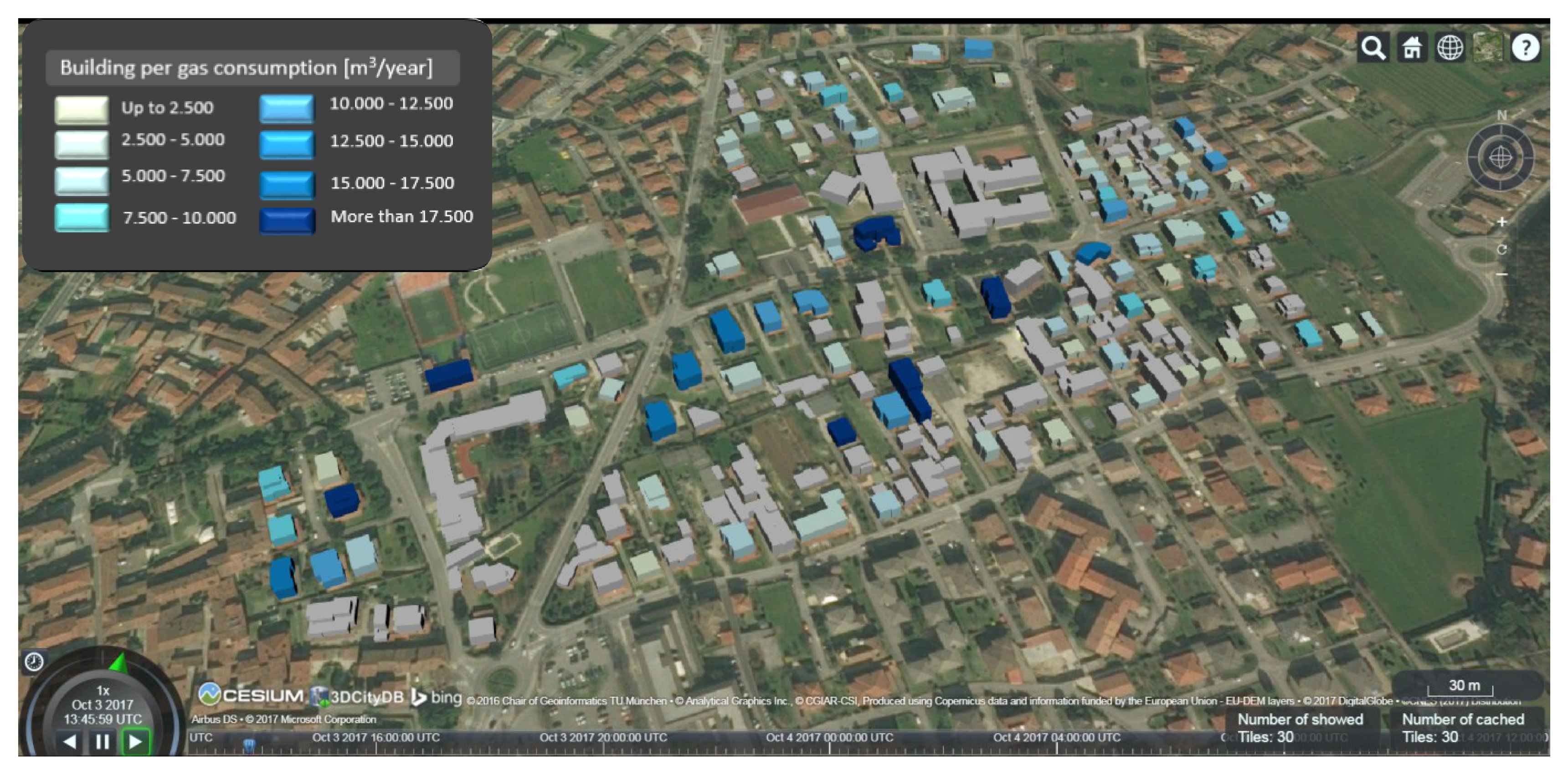
The EPCs and the actual energy consumption values were used to validate, as far as possible, the energy demand estimation. Energy consumption data are reported for every Point-of-Delivery (POD) registered in energy providers’ databases. In order to relate utility connections and buildings, the information that is associated to each POD was aggregated according to the address. As previously mentioned, addresses in these data sets are not structured and they are sometimes incomplete (e.g., the house number is missing). Thus, it was not always possible to associate consumption data to the correct building. As a result, gas consumption data were available only for 77 of the 154 buildings in the study area. Domestic hot water (DHW) and cooking consumptions were deducted from the total amount of consumed gas, in order to derive the portion of gas used for heating only. The equivalent amount of energy needed to obtain 50 l/person/day of DHW and 150 kWh/year/person for cooking was derived from the total gas consumption.

3.2. Parameters and Assumptions for the Energy Demand Calculation

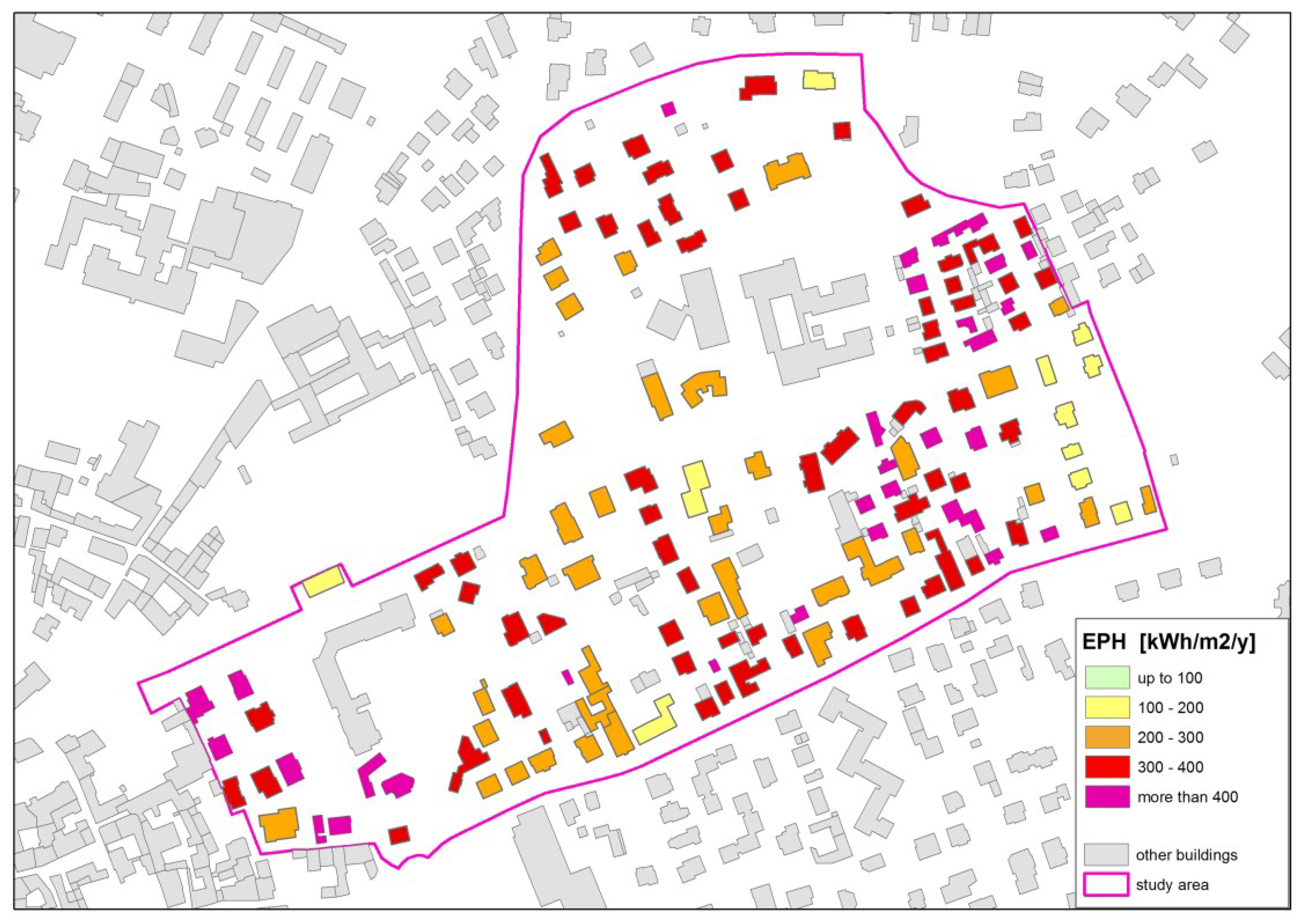
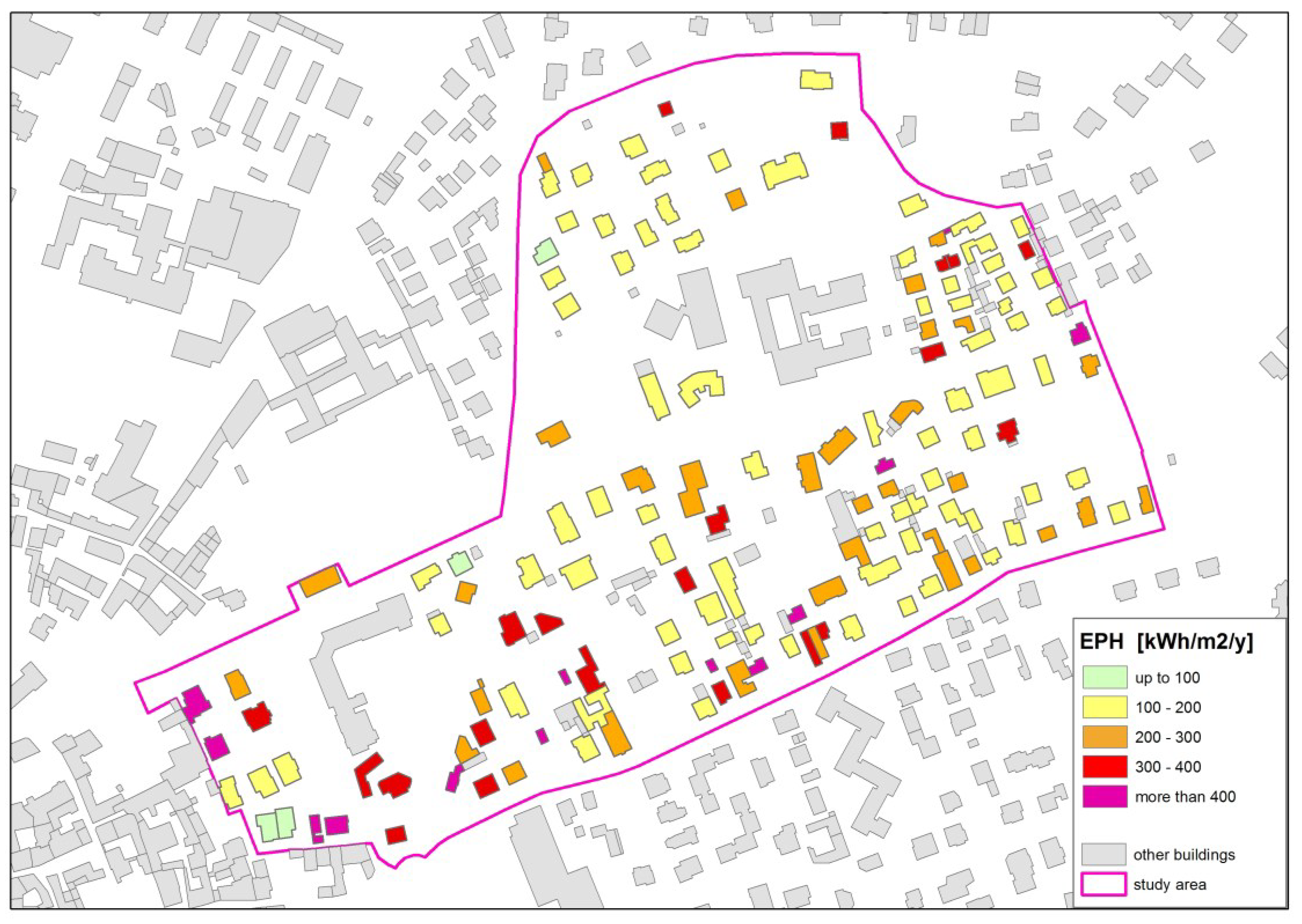
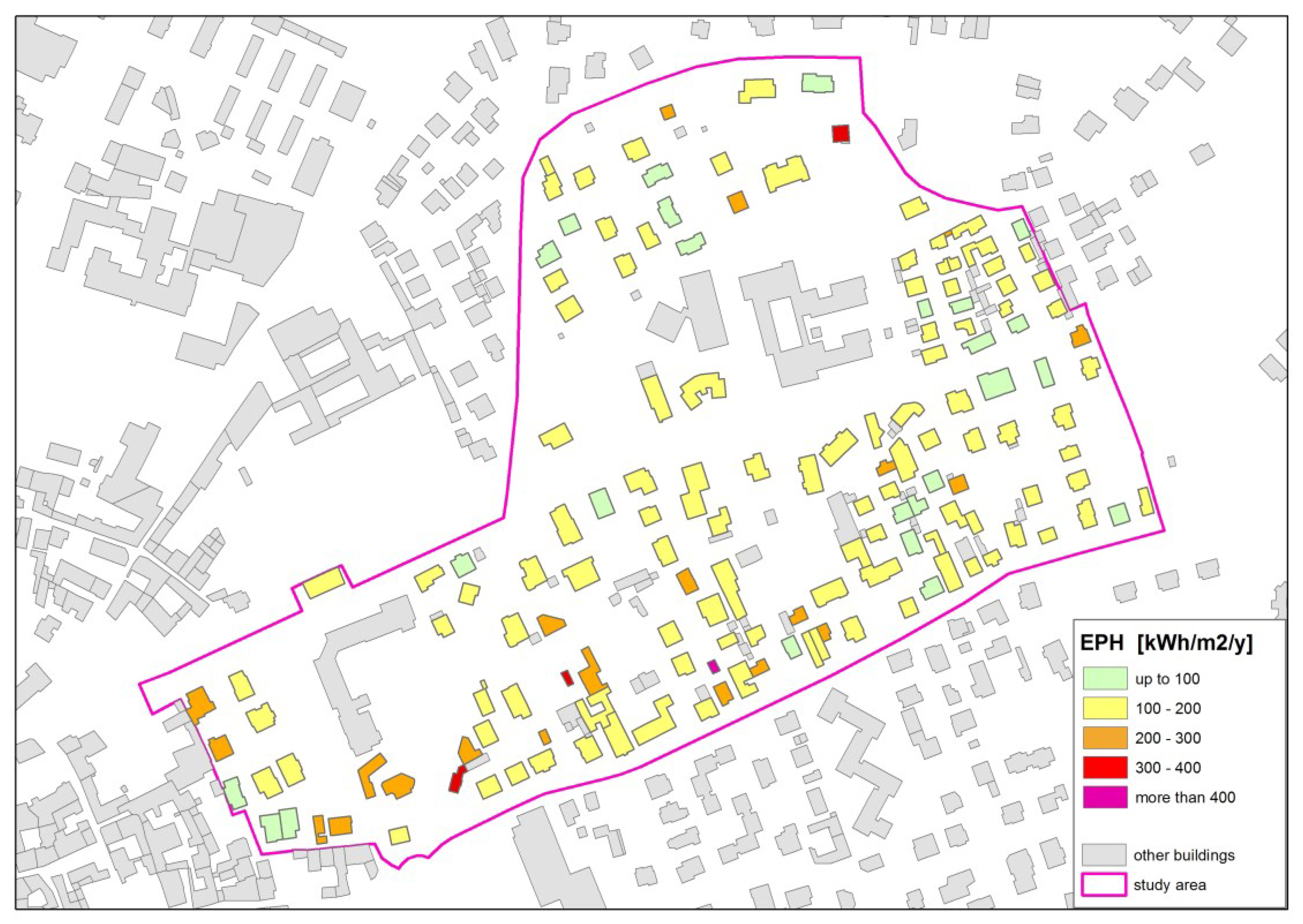
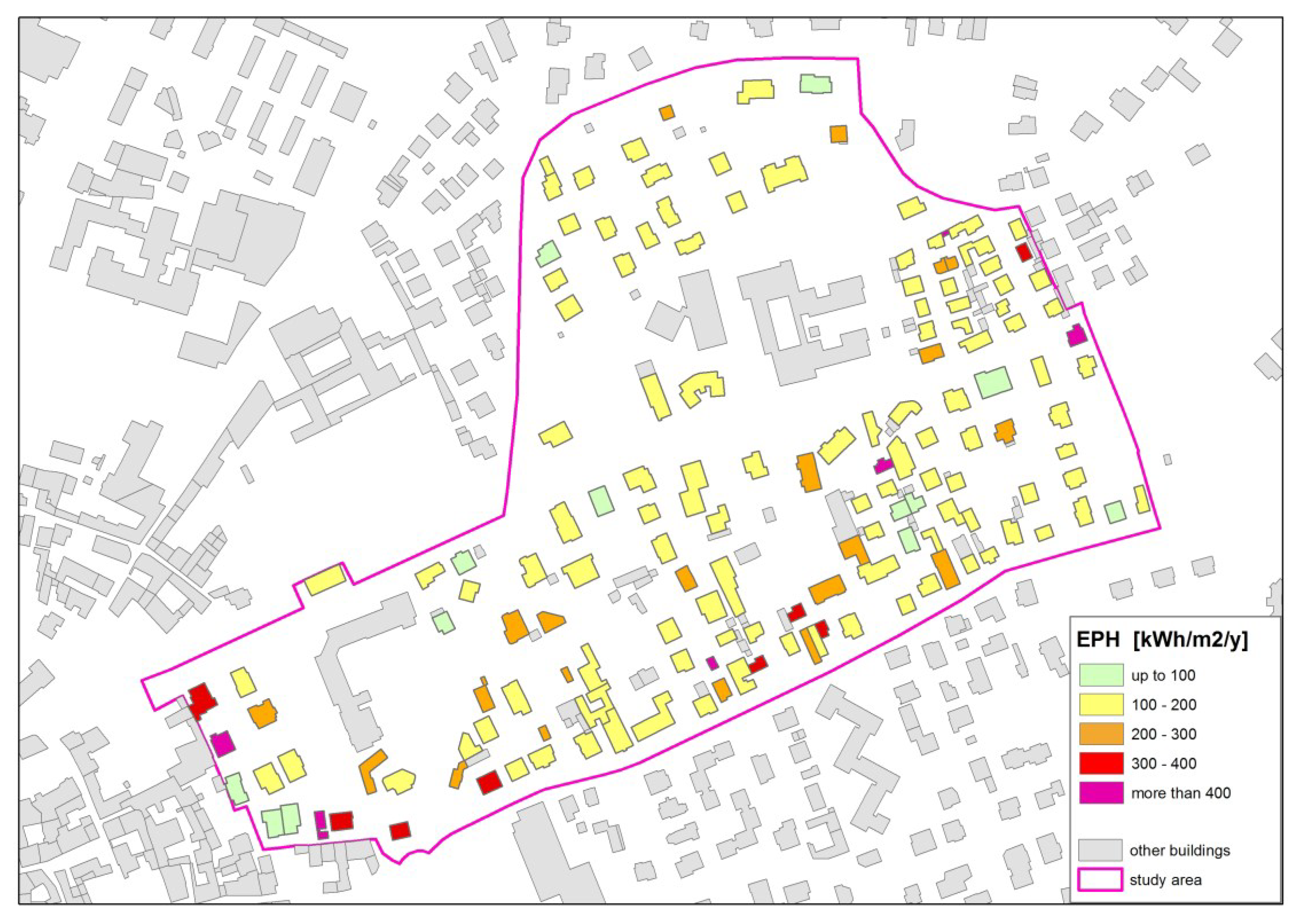
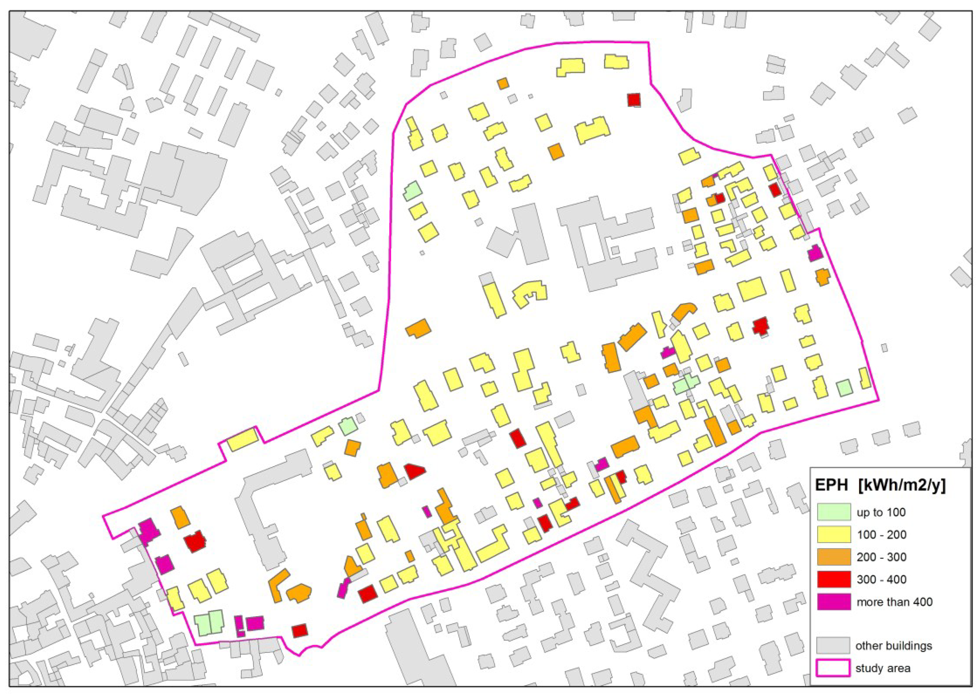
The results of the two different estimations are shown in Figure 7 and Figure 8: a general decrease in EPH values is evident when energy analysis is computed with DP2.

In order to check whether this decrease really corresponds to a more accurate evaluation, a comparison with other data sources (i.e., EPC values and real consumption values) was carried out.

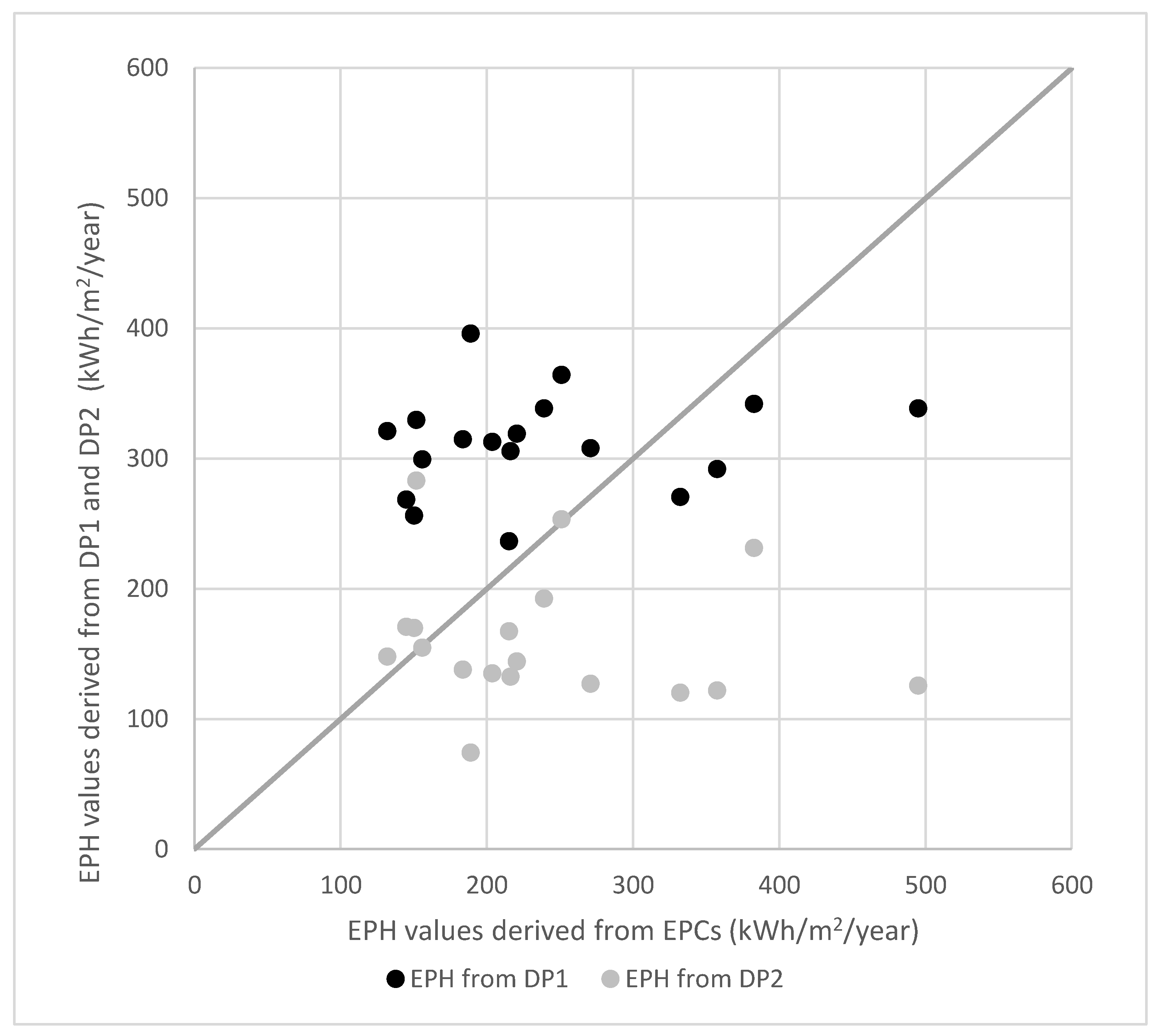
For 18 buildings within the study area where EPCs were available, energy values obtained from both data packages DP1 and DP2 were compared with EPC values. EPCs are generally the result of a detailed, on-site inspection accomplished by an expert professional. The performance values that were reported in these certificates are expected to be accurate and are obtained by following a methodology similar to the one used in this article.

These 18 buildings host 63 residential and 13 non-residential units. A total of 135 residents live there according to the Civil Registry. The small size of the sample is due to the scarce availability of EPC covering the entire buildings at the time that this work was carried out.

Nevertheless, the results of a comparison between the EPC values and the ones estimated from packages DP1 and DP2 are plotted in Figure 9 and are summarized in

Table 7. Comparison of Energy Performance for Heating (EPH) values (kWh m⁻²·year⁻¹).

Building ID	EPC	DP1	DP2	Consumption	Deviation from EPC Values
					DP1	%	DP2	%	CONS.	%
5950	150.1	256.1	169.9	33.2	106.0	70.6%	19.8	13.2%	−116.9	−77.9%
4928	131.8	321.2	147.8	34.8	189.4	143.7%	15.9	12.1%	−97.1	−73.6%
6940	220.2	319.2	144.1	48.6	99.0	45.0%	−76.2	−34.6%	−171.6	−77.9%
5860	188.8	395.9	74.1	85.0	207.1	109.7%	−114.7	−60.8%	−103.8	−55.0%
6831	155.7	299.5	154.9	95.7	143.9	92.4%	−0.8	−0.5%	−60.0	−38.5%
4930	183.4	314.8	137.8	138.3	131.4	71.7%	−45.5	−24.8%	−45.1	−24.6%
4815	215.9	305.7	132.4	145.7	89.8	41.6%	−83.5	−38.7%	−70.2	−32.5%
5802	214.9	236.5	167.4	151.3	21.5	10.0%	−47.5	−22.1%	−63.6	−29.6%
7151	357.3	291.9	121.9	154.4	−65.4	−18.3%	−235.4	−65.9%	−202.9	−56.8%
4918	144.7	268.4	170.7	159.6	123.7	85.5%	26.0	18.0%	15.0	10.3%
5825	203.6	312.8	135.1	177.9	109.2	53.6%	−68.5	−33.7%	−25.7	−12.6%
6070	332.0	270.5	120.2	207.2	−61.5	−18.5%	−211.8	−63.8%	−124.8	−37.6%
6093	270.8	307.8	127.1	226.8	37.0	13.7%	−143.7	−53.1%	−44.0	−16.3%
6866	239.0	338.7	192.6	239.6	99.7	41.7%	−46.4	−19.4%	0.6	0.3%
5761	382.5	341.9	231.2	289.1	−40.5	−10.6%	−151.2	−39.5%	−93.4	−24.4%
7440	494.7	338.5	125.5	305.8	−156.3	−31.6%	−369.2	−74.6%	−189.0	−38.2%
6068	151.5	329.6	283.2	405.9	178.1	117.5%	131.6	86.8%	254.4	167.9%
8246	250.9	364.2	253.2	472.9	113.2	45.1%	2.3	0.9%	222.0	88.5%
RMSE					121.0		136.6		128.2
MIN	131.8	236.5	74.1	33.2		−31.6%		−74.6%		−77.9%
MAX	494.7	395.9	283.2	472.9		143.7%		86.8%		167.9%
AVG	250.4	314.7	160.7	206.5		47.93%		−22.19%		−18.25%
MEDIAN	215.4	310.3	136.5	168.8		45.05%		−29.25%		−31.05%

. For each available EPC (its value is represented on the x-axis), the corresponding values computed from DP1 and DP2 are represented on the y-axis in blue and orange, respectively. The dashed line in the graph represents the (ideal) condition of perfect coincidence. First of all, this plot shows that DP1 values are generally higher than the corresponding DP2 values. Both sets of values are rather scattered and, with regard to the EPC values, their root mean squared errors (RMSE) yield rather similar values (121.0 kWh·m⁻²·year⁻¹ and 136.6 kWh·m⁻²·year⁻¹, respectively), but the average of the deviations is 40.5% for DP1 and −26.6% for DP2. In other words, the DP1 data lead to results that generally overestimate the EPCs, especially for efficient buildings (lower EPC values), while DP2 data lead to results that generally underestimate the EPC values.

However, as consumption values were available for the 18 buildings, these were also analysed with regards to the EPC values, as reported in Table 7. To enable such a comparison, the amount of gas consumption of each building was transformed in specific energy consumption by applying a lower calorific value (9.6 MJ/kg). In this case, the RMSE yields 128.2 kWh·m⁻²·year⁻¹ (a similar value as the previous two), and an average deviation of −11.1%. Given the small size of the sample, these results must be taken with care, as such high variability in terms of single building is well known in the literature and from other similar experiences [41,42].

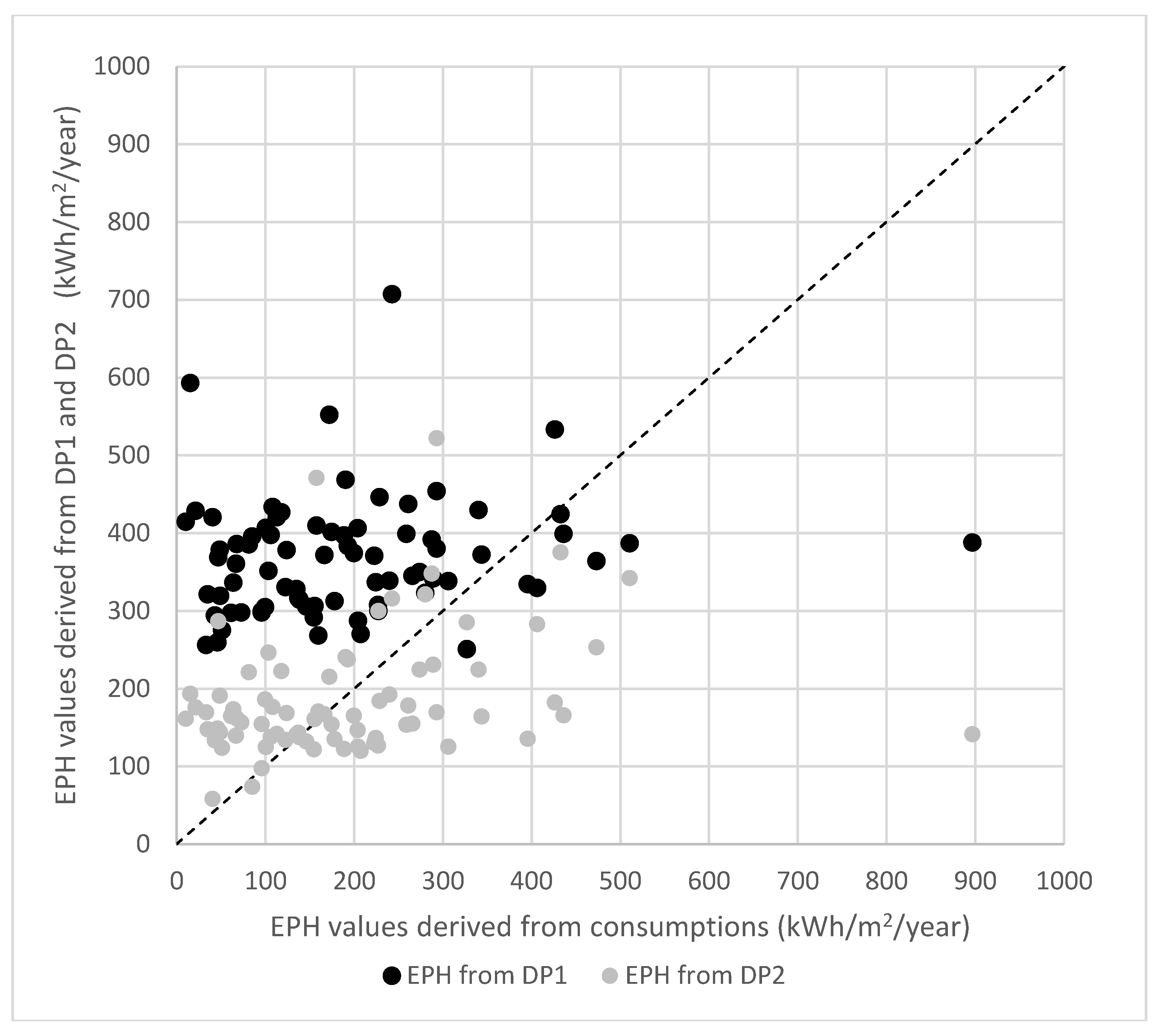
In order to (partially) overcome the lack of additional EPCs for a more robust validation of the model, a comparison between values obtained from packages DP1 and DP2 and the specific energy consumption (obtained from the annual gas consumption, as previously explained) was carried out on a larger sample of 77 out of 154 buildings, for which these data were available. These buildings host 163 residential units, 40 non-residential units, and 344 residents recorded at the Civil Registry. The difference between the estimated energy demand (from both packages DP1 and DP2) and the gas consumption was computed for this new sample.

Figure 10 shows the scatter plot and Appendix A contains a detail information record for each building. Globally, the RMSE of DP1 and DP2 yield 233.8 kWh·m⁻²·year⁻¹ and 142.5 kWh·m⁻²·year⁻¹, while the average deviations are 311.3% and 85.5%, respectively. In this case, DP2 overall leads to better results with respect to DP1.

A third analysis was carried out by computing first the yearly energy consumption for heating per each building (in MWh/year) by using packages DP1 and DP2, respectively. Subsequently, the values for the whole study area were aggregated and, eventually, compared to corresponding data obtained from the actual gas consumption (see Appendix A for details). The reason for this aggregation step is to reduce (or smooth out) the already mentioned local variability at building level due to specific users’ behaviours in terms of actual consumption. In such a case, DP1 and DP2 led to 8668.2 MWh/year and 4729.8 MWh/year, respectively. When compared to the actual 4786.9 MWh/year, the differences are 81.1% for DP1 and just −1.2% for DP2. This is another confirmation of the better suitability of DP2 with respect to DP1 scenario.

The table in Appendix A shows how, at the building level, deviations of the estimations from packages DP1/DP2 and the actual consumption may be sometimes significant: in general, the comparison with real consumption values and the ones that were obtained from package DP2 shows a better correspondence than in the case of package DP1. This outcome shows that an increase in the building data accuracy is reflected also in a more effective usability of such data in practical applications. The presence of some considerable deviations at building level is probably due to buildings with mixed use or predominantly non-residential function. Indeed, these other functions may not be distinguished from the residential function on the basis of the current adopted model. At district scale, the estimations differ from real consumption by approximately 1.2% only (in the case of DP2). The energy analysis computed with package DP2 may be considered therefore as a sort of “massive energy labelling operation” accomplished for all residential buildings within the study area.

3.3. Retrofitting Scenarios

Different retrofitting strategies were considered to improve the energy efficiency at a district level. The idea is to highlight the renovation and energy saving potential at macro scale that could help in triggering a systemic intervention at district/city scale. This would create the chance to take advantages from scale economies and to consider the possibility of installing local energy generation plants, with a consequent re-design of the public spaces, such as roads and green areas.

Several retrofitting scenarios were evaluated in compliance with the current national energy requirements for refurbishment. Since the substitution of the boiler is the option that is normally adopted by private owners due to the lower cost and to the short payback time, district-scale retrofitting scenarios excluded the boiler improvement as a scenario per se. Retrofitting options were computed for three alternative and more involved measures, which are also more expensive:

• “Wall insulation” scenario (U_wall = 0.3 W/(m²K));
• “Roof insulation” scenario (U_roof = 0.22 W/(m²K)); and,
• “Windows improvement” scenario (U_wind = 1.9 W/(m²K)).

Values in brackets represent the corresponding thermal transmittances.

Moreover, a “Total retrofitting” scenario was computed by merging all the above-mentioned measures and including the installation of condensing boilers with a generation efficiency factor of 0.95. In such a case, the improvement of the boiler efficiency was also considered, while taking into account the installation of condensation boilers in place of standard ones.

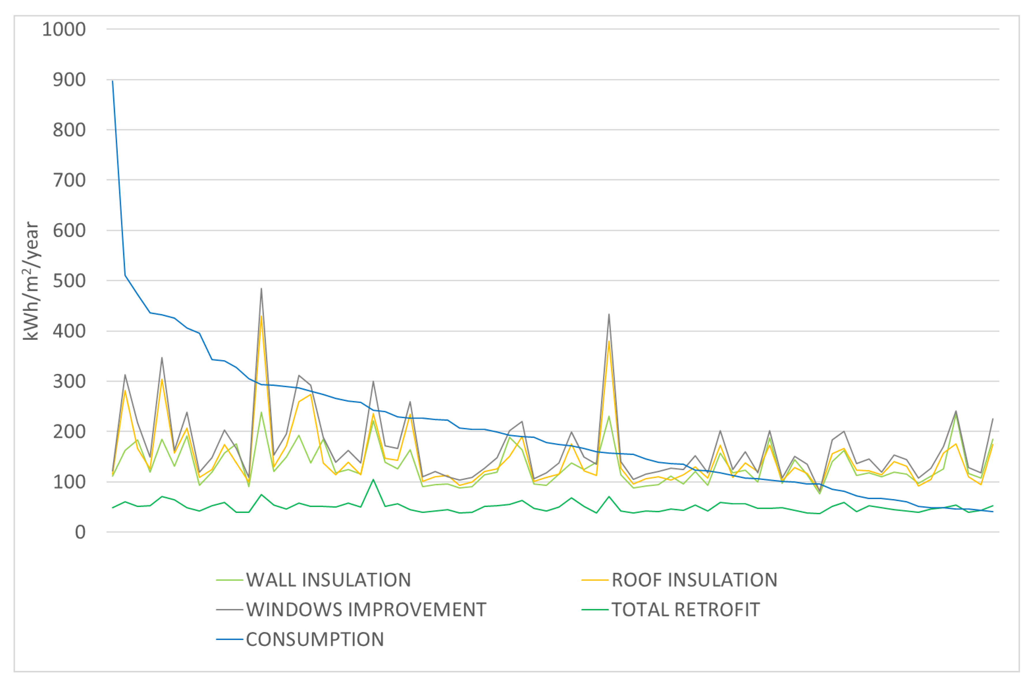
The energy improvements per each of the four scenarios are displayed in Figure 11 and mapped in Figure 12, Figure 13, Figure 14 and Figure 15. Each scenario partially improves the existing situation. However, the “Total retrofitting” is by far the best option in terms of energy saving. When considering the assumptions and simplifications in the Gavardo focus area (e.g., no shading evaluation, same window-to-wall ratio for all orientations, forfeit evaluation of thermal bridges, etc.) the most efficient scenario is the one consisting in the “Wall insulation”, as there are not wide glazed surfaces and opaque envelopes are prevalent. The “Window replacement” scenario has the lowest impact due to the low-rise residential typology of houses, characterized by few glazed surfaces.

Costs of the proposed retrofitting scenarios were estimated for each building according to the following criteria:

• thermal transmittance values for “Wall insulation”, “Roof insulation”, and “Window improvement“ scenarios were chosen in accordance to the current requirements defined for the admission to public incentives (U_wall = 0.3; U_roof = 0.22; U_wind = 1.9, all values in W m⁻²K⁻¹);
• given the previous point, the chance to obtain public incentives covering 65% of the intervention costs;
• for the “Wall insulation” scenario, by considering side works on the building layout and finishes, costs were charged an additional 20%; and,
• average gross cost of gas (considering taxes): 0.71 €/m³.

All the costs computed per every building within the focus area were aggregated, obtaining the total cost of intervention at district level for the different retrofitting scenarios. Payback time and costs per each scenario are summarized in

Table 8. Costs associated to retrofitting scenarios and payback time.

Scenario	Cost with Incentives (€)	Cost without Incentives (€)	Payback Time with Incentives (years)	Payback Time without Incentives (years)
Wall insulation	1,254,118	3,583,195	5.9	16.8
Roof insulation	525,655	1,501,870	3.3	9.6
Window improvement	1,117,948	3,194,136	16.5	47.2
Total retrofit	3,446,319	9,846,625	6.0	17.1

while potential savings are reported in

Table 9. Savings associated to retrofitting scenarios.

Scenario	Gas Saving (MWh/year)	Gas Saving (m3/year)	Energy Cost Saving (€/year)	CO2 Saving (t/year)
Wall insulation	2912.4	300,251	213,178	630.5
Roof insulation	2144.0	221,027	156,929	464.2
Window improvement	924.3	95,293	67,658	200.1
Total retrofit	7626.9	786,283	558,261	1651.2

. As expected, the option that provides the highest annual energy, money, and CO₂ savings is the “Total retrofitting” scenario, but the required investment is almost three times as compared to “Wall insulation” scenario, and five time higher than “Roof insulation” scenario, respectively. The “Wall insulation” and the “Roof insulation” scenarios are the two options with the shortest payback time, but the latter involves much lower costs. “Window improvement” scenario by itself does not represent a feasible option considering the importance of the investment and the long payback time when compared to the potential savings.

4. Conclusions

The research described in this paper has demonstrated how the implementation of a Building Information System (BIS) in an Italian local administration could be profitably used to pursuit collective interests. Building data sources, available at the public level, were thoroughly analysed with regard to their contents and structure. A theoretical path to relate existing, unlinked databases was outlined. In order to test the actual viability of data integration in real-life conditions, the creation of a BIS was tested in a case study area. This test allowed for detecting current shortcomings that are related to the quality of building information, demonstrating how the complete integration of building data is not always achievable in an automatic way. This task would require the stronger involvement of all authorities in charge of public data management to improve the quality of existing information.

Although it can be seen as a time-consuming task, the work done in the case of Gavardo municipality shows how the creation of a BIS may provide a ready-to-use information package to be exploited by different applications. The availability of integrated building data allowed for proceeding with the automatic computation of the primary energy demand for heating in a district of more than 150 buildings. The main scope of this application was to highlight a retrofitting potential at the macro scale that could help trigger a systemic renovation intervention at district/city scale. The accuracy of the obtained energy estimates can be considered to be sufficient at district scale, however it clearly requires further investigation and refinement at the building level, as the current results show. Nevertheless, the good correspondence between estimated and measured energy values at the district scale is a positive indicator, remarking how the availability of integrated building data may enable the development of tools and methods to support public policy makers in the pursuit of sustainability goals.

In addition, the building data were modelled according to CityGML in order to test how existing archives may be effectively mapped to this standard data model, as well as to evaluate the chance to profitably adopt an international and widely recognized standard. First, a base city model was created from the BIS through an extraction, transformation, and load workflow. Thanks to the already available (free and open-source) 3D City Database, all data could be stored in a relational, CityGML-compliant database. In line with the energy analysis, the implementation of the Energy ADE was also tested and energy-related parameters were modelled for all buildings within the focus area. This experience demonstrates how the creation of a standard-compliant city model is achievable. The Gavardo city model is one of the few examples in Italy of integrated and harmonized building data, modelled according to an open, internationally recognized standard, and the first in Italy to test and take advantage of the Energy ADE. Given the adoption of publicly available data, this experience may be replicated in other Italian local administrations.

Further development of the research will aim to improve the degree of automation, to facilitate the integration of building data, and to improve seamless update mechanism to guarantee good data quality. From this point-of-view, an ontology-based approach for data integration should allow to overcome problems due to the materialization of integrated data, easing the retrieval of updated information. Also, the slowly but constantly increasing availability of BIM (Building Information Modelling) models will be an opportunity to widen the range of standardized building data sources.

Nevertheless, the creation of a BIS does not have to be interpreted as a finish line, but rather as a starting point for the reorganization and the qualitative improvement of public information on buildings. The integration and harmonisation of heterogeneous data sources represents a good chance to test data coherence, solving possible inconsistencies through the comparison with the real world. The final goal of creating such a hub of integrated information is the actual matching between data and reality. Thus, the creation of a BIS is a chance to trigger the definition of efficiency strategies in the management of public data.

References

1. Tagliabue, L.C.; Manfren, M.; Ciribini, A.L.C.; De Angelis, E. Tuning energy performance simulation on behavioural variability with inverse modelling: The case of Smart Campus Building. In Proceedings of the Sustainable Built Environment (SBE) Regional Conference, Expanding Boundaries: Systems Thinking for the Built Environment, Zurich, Switzerland, 13–17 June 2016; pp. 142–147. [Google Scholar]
2. Bignami, D.F. Towards a Territorial Multi-Disaster Buildings’ Resistance Certification; Springer Science & Business: Berlin, Germany, 2014. [Google Scholar]
3. Pasini, D.; Mastrolembo Ventura, S.; Rinaldi, S.; Bellagente, P.; Flammini, A.; Ciribini, A.L.C. Exploiting Internet of Things and Building Information Modeling Framework for Management of Cognitive Buildings. In Proceedings of the IEEE 2nd International Smart Cities Conference (ISC2 2016) “Improving the Citizens Quality of Life”, Trento, Italy, 12–15 September 2016; pp. 12–15. [Google Scholar]
4. Pasquinelli, A.; Guzzetti, F. Knowledge for Intelligence: Discussing the state and the role of building data in Italy. ISPRS Ann. Photogramm. Remote Sens. Spat. Inf. Sci. 2016, 11–18. [Google Scholar] [CrossRef]
5. Caputo, P.; Pasetti, G. Overcoming the inertia of building energy retrofit at municipal level: The Italian challenge. Sustain. Cities Soc. 2015, 15, 120–134. [Google Scholar] [CrossRef]
6. Van Eekelen, H. Large Scale Basemap as an Authentic Registration? GIM Int. 2001, 15, 53–55. [Google Scholar]
7. Van der Molen, P. Partnerships for better service Public-Private and Public-Public Partnerships to achieve better service to customers in The Netherlands. In United Nations Economic Commission for Europe, Working Party on Land Administration; UNECE: Vienna, Austria, 2002. [Google Scholar]
8. Bakker, N.J.; Van der Vegt, H.H.; Bruns, B. Dutch NMCA launches Open data. In Proceedings of the 26th International Cartographic Conference, Dresden, Germany, 25–30 August 2013. [Google Scholar]
9. Van den Brink, L.; Stoter, J.; Zlatanova, S. Establishing a national standard for 3D topographic data compliant to CityGML. Int. J. Geogr. Inf. Sci. 2012, 27, 92–113. [Google Scholar] [CrossRef]
10. Hawerk, W. ALKIS—Germany’s Way into A Cadastre for the 21st Century. In Proceedings of the FIG Working Week 2001, Seoul, Korea, 6–11 May 2001. [Google Scholar]
11. Chester, S.; De Lathouwer, B. Smart Cities driving integration of BIM & geospatial. Geospatial World Magazine, 5 July 2016. Available online: https://www.geospatialworld.net/article/building-greater-britain-integration-bim-gi/(accessed on 10 January 2019).
12. Ordnance Survey. Integration of BIM and GIS in the United Kingdom. Geospatial World Magazine, 8 July 2016. Available online: https://www.geospatialworld.net/article/building-greater-britain-integration-bim-gi/(accessed on 10 January 2019).
13. Conejo Fernandez, C. Spanish cadastral Information system. Current status and I.T. renovation strategy. Catastro 2016, 48, 233–243. [Google Scholar]
14. Olivares García, J.M.; Virgós Soriano, L.I.; Velasco, M.V. A 3D Modeling and Representation of the Spanish Cadastral Cartography. In Proceedings of the 2nd International Workshop on 3D Cadastres, Delft, The Netherlands, 16–18 November 2011. [Google Scholar]
15. Pasquinelli, A. The Creation of a Citywide Building Information System: Criticalities and Potentialities of Public Information on Buildings. Ph.D. Thesis, Politecnico Milano, Milan, Italy, 2017. [Google Scholar]
16. Scaioni, M.; Guastamacchia, E.; Crimella, E. The Topographic Db as a tool for land management and government: The ‘Provincia di Lecco project’. In Representation of Geographical Information for Planning; Caglioni, M., Scarlatti, F., Eds.; Esculapio: Bologna, Italy, 2009; pp. 29–38. [Google Scholar]
17. European Parliament. Directive 2007/2/EC Establishing an Infrastructure for Spatial Information in the European Community (INSPIRE); European Parliament: Brussels, Belgium, 2007. [Google Scholar]
18. Ministero Delle Finanze. Decreto Ministeriale N. 28 (2 Gennaio 1998)—Regolamento Recante Norme in Tema di Costituzione del Catasto dei Fabbricati e Modalità di Produzione ed Adeguamento della Nuova Cartografia Catastale; Ministero Delle Finanze: Rome, Italy, 1998.
19. Tonelli, E.; Guzzetti, F.; Baragetti, E.; Colombo, P.F.; Caspani, P.; Viskanic, P.; Scaioni, M. Un percorso per l’integrazione dei Database Topografici con le informazioni del Catasto dei Terreni nelle zone ‘a perimetro aperto’. In Proceedings of the 20th Conferenza Nazionale ASITA, Cagliari, Italy, 8–10 November 2016; pp. 623–630. [Google Scholar]
20. Brovelli, M.A.; Zamboni, G. The usability of vectorization and a new point matching procedure as first step in conflating raster and vector maps. Int. Arch. Photogramm. Remote Sens. Spat. Inf. Sci. 2006, 36, 85–91. [Google Scholar]
21. Open Geospatial Consortium. OGC City Geography Markup Language (CityGML) Encoding Standard; OGC 12-019—Version 2.0.0; Open Geospatial Consortium: Wayland, MA, USA, 2012. [Google Scholar]
22. Kolbe, T.H. Representing and Exchanging 3D City Models with CityGML. In 3D Geo-Information Sciences; Lee, J., Zlatanova, S., Eds.; Springer: Berlin, Germany, 2009. [Google Scholar]
23. buildingSMART Website. Available online: www.buildingsmart-tech.org (accessed on 24 November 2018).
24. gbXML Website. Available online: www.gbxml.org (accessed on 24 November 2018).
25. INSPIRE—Infrastructure for Spatial Information in Europe. Data Specification on Buildings; Technical Guidelines (D2.8.III.2_v3.0); INSPIRE: Brussels, Belgium, 2013. [Google Scholar]
26. Biljecki, F.; Stoter, J.; Ledoux, H.; Zlatanova, S.; Çöltekin, A. Applications of 3D City Models: State of the Art Review. ISPRS Int. J. Geo-Inf. 2015, 4, 2842–2889. [Google Scholar] [CrossRef] [Green Version]
27. Agugiaro, G.; Benner, J.; Cipriano, P.; Nouvel, R. The Energy Application Domain Extension for CityGML: Enhancing interoperability for urban energy simulation. Open Geospat. Data Softw. Stand. 2018, 3, 2. [Google Scholar] [CrossRef]
28. Safe Software website. Available online: www.safe.com (accessed on 31 October 2018).
29. Cesium website. Available online: https://cesiumjs.org/ (accessed on 24 November 2018).
30. Agugiaro, G. Enabling “energy-awareness” in the semantic 3D city model of Vienna. ISPRS Ann. Photogramm. Remote Sens. Spat. Inf. Sci. 2018, 4, 81–88. [Google Scholar] [CrossRef]
31. Benner, J.; Geiger, A.; Häfele, K.H. Virtual 3D City Model Support for Energy Demand Simulations on City Level—The CityGML Energy Extension. In Proceedings of the REAL CORP Conference, Hamburg, Germany, 22–24 June 2016; pp. 777–786. [Google Scholar]
32. Corrado, V.; Ballarini, I.; Corgnati, S.P. Building Typology Brochure—Italy. Fascicolo Sulla Tipologia Edilizia Italiana (Nuova Edizione); Politecnico di Torino: Turin, Italy, 2014. [Google Scholar]
33. Energy ADE Documentation. Available online: https://github.com/cstb/citygmlenergy (accessed on 24 November 2018).
34. Strzalka, A.; Bogdahn, J.; Eicker, U. 3D City Modelling for Urban Scale Heating Energy Demand Forecasting. HVACR Res. 2010, 17, 526–539. [Google Scholar]
35. Kaden, R.; Kolbe, T. City-Wide Total Energy Demand Estimation of Buildings Using Semantic 3D City Models and Statistical Data. Int. Arch. Photogramm. Remote Sens. Spat. Inf. Sci. 2013, 2, 27–29. [Google Scholar] [CrossRef]
36. Nouvel, R.; Zirak, M.; Dastageeri, H.; Coors, V.; Eicker, U. Urban energy analysis based on 3D city model for national scale applications. In Proceedings of the 5th German-Austrian IBPSA Conference, Aachen, Germany, 22–24 September 2014; pp. 83–90. [Google Scholar]
37. Dall’O’, G.; Galante, A.; Pasetti, G. A methodology for evaluating the potential energy savings of retrofitting residential building stocks. Sustain. Cities Soc. 2012, 4, 12–21. [Google Scholar] [CrossRef]
38. Caputo, P.; Costa, G.; Ferrari, S. A supporting method for defining energy strategies in the building sector at urban scale. Energy Policy 2013, 55, 261–270. [Google Scholar] [CrossRef]
39. Di Turi, S.; Stefanizzi, P. Energy analysis and refurbishment proposals for public housing in the city of Bari. Italy. Energy Policy 2015, 79, 58–71. [Google Scholar] [CrossRef]
40. Ente Nazionale Italiano di Unificazione UNI/TS 11300-1:2014: Energy Performance of Buildings—Part 1: Evaluation of Energy Need for Space Heating and Cooling. Available online: http://store.uni.com/catalogo/index.php/uni-ts-11300-1-2014.html?josso_back_to=http://store.uni.com/josso-security-check.php&josso_cmd=login_optional&josso_partnerapp_host=store.uni.com. (accessed on 10 January 2019).
41. Nouvel, R.; Zirak, M.; Coors, V.; Eicker, U. The influence of data quality on urban heating demand modeling using 3D city models. Comput. Environ. Urban Syst. 2017, 64, 68–80. [Google Scholar] [CrossRef]
42. Fonseca, A.J.; Schlueter, A. Integrated model for characterization of spatiotemporal building energy consumption patterns in neighborhoods and city districts. Appl. Energy 2015, 142, 247–265. [Google Scholar] [CrossRef]
Figure 1. Example of a single building in the Topographic Database (TDB) (on the left), subdivided in four properties in the cadastre (on the right). Image source: authors.
Ijgi 08 00027 g001
Figure 2. Position of the province of Brescia in Italy (on the left). The municipality of Gavardo within the Sabbia Valley (on the right), which was selected as case study area. Image source: authors.
Ijgi 08 00027 g002
Figure 3. The study area in the municipality of Gavardo. Image source: authors.
Ijgi 08 00027 g003
Figure 4. Schematic view of the data manipulation process implemented in Feature Manipulation Engine 2017 (FME). Image source: authors.
Ijgi 08 00027 g004
Figure 5. Three-dimensional (3D) view of the Gavardo city model published on the web using the free virtual globe library Cesium. Image source: authors.
Ijgi 08 00027 g005
Figure 6. Buildings classified according to the measured gas consumption and published in the free virtual globe library Cesium. Image source: authors.
Ijgi 08 00027 g006
Figure 7. Heating energy demand computed with data package DP1. Image source: authors.
Ijgi 08 00027 g007
Figure 8. Heating energy demand computed with data package DP2. Image source: authors.
Ijgi 08 00027 g008
Figure 9. Comparison of results obtained from packages DP1 and DP2 with respect to the energy performance certificates (EPCs) of 18 buildings in the study area. Image source: authors.
Ijgi 08 00027 g009
Figure 10. Comparison of results that were obtained from packages DP1 and DP2 with respect to consumptions of 77 buildings in the study area. Image source: authors.
Ijgi 08 00027 g010
Figure 11. Comparison of retrofitting scenarios. Please note that the use of the line chart is intended only to facilitate the comparison, but building values do not correlate to one other. Image source: authors.
Ijgi 08 00027 g011
Figure 12. Estimated energy consumption for the retrofitting scenario “Wall insulation”. Image source: authors.
Ijgi 08 00027 g012
Figure 13. Estimated energy consumption for the retrofitting scenario “Roof insulation”. Image source: authors.
Ijgi 08 00027 g013
Figure 14. Estimated energy consumption for the retrofitting scenario “Windows improvement”. Image source: authors.
Ijgi 08 00027 g014
Figure 15. Estimated energy consumption for the retrofitting scenario “Total retrofitting”. Image source: authors.
Ijgi 08 00027 g015