Article

Adaptive Non-Negative Geographically Weighted Regression for Population Density Estimation Based on Nighttime Light

1
Department of Geomatics, National Cheng Kung University, Tainan 70101, Taiwan
2
Graduate Institute of National Development, National Taiwan University, Taipei 10617, Taiwan
*
Author to whom correspondence should be addressed.
ISPRS Int. J. Geo-Inf. 2019, 8(1), 26; https://doi.org/10.3390/ijgi8010026
Submission received: 14 November 2018 / Revised: 3 January 2019 / Accepted: 9 January 2019 / Published: 12 January 2019

Abstract

:
Nighttime light imagery provides a perspective for studying urbanization and socioeconomic changes. Traditional global regression models have been applied to explore the nonspatial relationship between nighttime lights and population density. In this study, geographically weighted regression (GWR) identifies the spatially varying relationships between population density and nighttime lights in mainland China. However, the rural population does not have a strong relationship with remote-sensing spectral features. The rural population estimation using nighttime light data alone easily identifies meaningless negative population density in the rural area. This study proposes an adaptive non-negative GWR (ANNGWR) to explore the spatial pattern of population density by using nonnegative constraints with an adaptive bandwidth of kernel. The ANNGWR solves the negative value of population density and serious overestimation of the western boundary. The result shows that the ANNGWR provides the best goodness-of-fit compared with linear regression and original GWR. This study applies Moran’s I index to prove that the ANNGWR substantially decreases the spatial autocorrelation of the model residual. The model offers a robust and effective approach for estimating the spatial patterns of regional population density solely on the basis of nighttime light imagery.

1. Introduction

Population density is a major index for measuring human development and assessing urbanization in urban areas. Gaining accurate and detailed population data is a complicated task in developing countries. This complication results not only from the expensive and time-consuming population data collection but also from the unwillingness of local governments (and the central government) to reveal the population data in every locality. During the economic marketization process in numerous developing countries, rural residents migrate rapidly to urban areas while government regulations on migration remain largely rigid. These unchanged regulations reflect governments’ hesitation in promoting human mobility (often for the purpose of social control), and in most cases, this situation considerably affects the release of government statistics on population. Hence, population survey data may have several missing values and sampling bias. Accordingly, to measure the detailed process of urbanization across different localities, researchers cannot only rely on local records. Satellite images here provide a useful global viewpoint. These data are helpful in tracing the detailed process of urbanization [1,2,3].
Using nighttime light imagery for studying urbanization and socioeconomic situations differs greatly from using conventional daytime light satellite remote sensing [1,2,3,4]. The U.S. Air Force’s Defense Meteorological Satellite Program/Operational Linescan System (DMSP/OLS) provides the nighttime light data. Previous studies have used the DMSP/OLS sensor to monitor nighttime lights from space and quantify the relationships between human activity and socioeconomic variables and nighttime brightness [1,2,3,4]. Nighttime lights have been extensively used to investigate spatial and temporal trends in various fields, e.g., economic activity [2], population density [1,3], energy use and carbon emissions [5], natural disasters [6], city light [7], regional development, light pollution, wildfires, and fishing. In the present study, we explore the spatial relationship between nighttime lights and population density. We use mainland China as an example to illustrate the relationship between nighttime lights and population survey data. China is one of the most populous countries in the world. The average population density in China in 2015 was 148.8 persons per square km. However, this number alone does not reveal how unevenly the Chinese population is distributed. Studies have found that China is heavily populated on the east coast [8]. The uneven distribution of the spatial population density has created difficulties for researchers in exploring the relationship between nighttime lights and population numbers. Most previous studies have used traditional global regression models and have not considered spatial heterogeneity [4,9,10]. Sun et al. [4] applied linear and power regression models to estimate the urban and rural population density. Bustos et al. [9] adopted a polynomial regression model to find the population change in Europe. Lo [10] used a logarithmic regression model to evaluate the population data in China at the provincial, city, and county levels. These studies have neglected the existence of spatial heterogeneity. To overcome this weakness, we utilize the geographically weighted regression (GWR) model [11], which is a local regression method for identifying spatially varying relationships between population density and nighttime lights in mainland China. Although the GWR can incorporate spatial heterogeneity, the regression sometimes results in invalid or meaningless predictions of the dependent variable. Specifically, the GWR model easily estimates meaningless negative population density in rural areas. A negative population number is problematic in interpretation. The rural population does not have a strong relationship with remote-sensing spectral features; thus, estimating the rural population distribution using the DMSP/OLS nighttime light data alone results in inaccurate data [4,12]. To address this problem, previous studies have estimated population density using nighttime light and land use data [4,12]. However, we consider only nighttime light data for the nonnegative least squares where no coefficients are allowed to be negative in the GWR framework without any data transformation, such as log transformation.
This study aims to identify the spatially varying relationships between regional population density data and nighttime light images in mainland China. We develop a statistical framework for using satellite data of nighttime lights to model the population density without any negative population values. Initially, the model considers the non-negative constrained GWR (NNGWR) for eliminating the negative population. The adaptive non-negative GWR (ANNGWR) model is then developed to adjust the bandwidth adaptively for estimating the nonnegative model coefficient. Finally, our proposed method compares favorably with OLS and the original GWR.

2. Materials and Methods

The nighttime light images used in this study are the DMSP/OLS global nighttime light data products in 2004, 2007, 2010, and 2013 from the National Oceanic and Atmospheric Administration (http://ngdc.noaa.gov/eog/download.html). The annual cloud-free composites of stable light data at each pixel are recorded as a digital number (DN) from 0 to 63 with a 1 km spatial resolution. For the target variable, 1,905 observations (Figure 1a) of the annual population at the county level were retrieved from the population survey published in the China Statistical Yearbook [13].
Every year, the government publishes the China Statistical Yearbook, which is a major source of the country’s various socioeconomic data. The Statistical Yearbook provides information at different levels of administrative divisions, and the county level is the lowest level with records. For population data, the government also conducts a national census every 10 years. As the census data are only released every 10 years, the annual population data published in the Statistical Yearbook are widely used in the field, especially those that focus on the evolution of population across years (e.g., reference [14]). Nonetheless, the population data of mainland China have several missing values (Figure 1b). In our model, we used the population data in the Statistical Yearbook as our target variable and the nighttime light imagery as the explanatory variable. The whole data were randomly separated into 70% and 30% for independent training and validation, respectively.
Figure 2 shows the flowchart of the ANNGWR model. The model is applied for estimating the coefficients of model between the nighttime lights and population data. In this study, the average DN values of nighttime light images and the population density of each county can be calculated.
All coefficients have to be positive values to avoid the negative population problem. Furthermore, the bandwidth was adaptively adjusted for the coefficient estimation in these models. After the fitting, the model coefficients in a spatial map were estimated by inverse distance weighting. Finally, the population density map was created on the basis of the nighttime light image and the estimated coefficients from the models. The models in the study are as follows: the OLS, original GWR, NNGWR considering only the nonnegative constraint, and ANNGWR considering the nonnegative constraint and adaptive kernel bandwidth.
GWR allows spatial coefficients to estimate the regression model [11], which can be expressed as
Y i   =   k β k ( u i , v i ) X i k + ε i
where Y i is the population density at each county (observation) i. k denotes the index of variables. X i k for k   =   1 represents the nighttime light information (average DN value) at observation i. β k ( u i , v i ) refers to the kth coefficient that varies with the spatial coordinates ( u i , v i ) at observation i. β 0 ( u i , v i ) indicates the intercept. β 1 ( u i , v i ) is the slope for nighttime light information in the model.
The estimated coefficient β ^ k ( u i , v i ) at each observation i is as follows:
β ^ k ( u i , v i )   =   [ X T W ( u i , v i ) X ] 1 X T W ( u i , v i ) Y
where W ( u i , v i ) is a spatial weight matrix based on the Euclidean and Gaussian distance decay-based functions. In each matrix element, the spatial weight at any observation is decided by the kernel. The most widely used kernel is the Gaussian kernel function.
w ( u i , v i ) j   =   e ( d i j / h ) 2
where d i j represents the Euclidean distance of variable values between the observation location i and its neighboring j. h denotes the bandwidth for each variable of the kernel Gaussian function. The optimal bandwidth is determined by the cross validation approach in this study [15]. Moreover, the optimal bandwidth is 0.3.
The nighttime light is often positively proportional to the population density, i.e., the positive value of the slope between population density and nighttime light. Thus, the NNGWR model is constrained to nonnegative coefficients. The NNGWR is the local model of least squares (Equation (4)). At any observation, the constrained least squares where the coefficients are not allowed to become negative were applied [16].
Min   X β Y i 2 s . t .   β k ( u i , v i ) 0
Accordingly, the ANNGWR consists of the following procedure.
Original GWR: estimate initial β k ( u i , v i ) by Equation (2);
h at observation i where initial β k ( u i , v i ) < 0 is adjusted iteratively;
Nonnegative GWR: estimate β k ( u i , v i ) by the constrained least squares [16] (Equation (4)).
The local bandwidth was adaptively adjusted when considering Equation (4) to prevent the coefficients from becoming less than zero. The kernel bandwidth was iteratively set to a small value if the regression coefficients within an active constraint were allowed to be positive.
The indices, e.g., R2, root mean square error (RMSE), and global and local Moran’s I [17], of model residuals were used for model validation in this study. The models were validated during the 4 years. However, one of them was a demo case in 2007.

3. Results

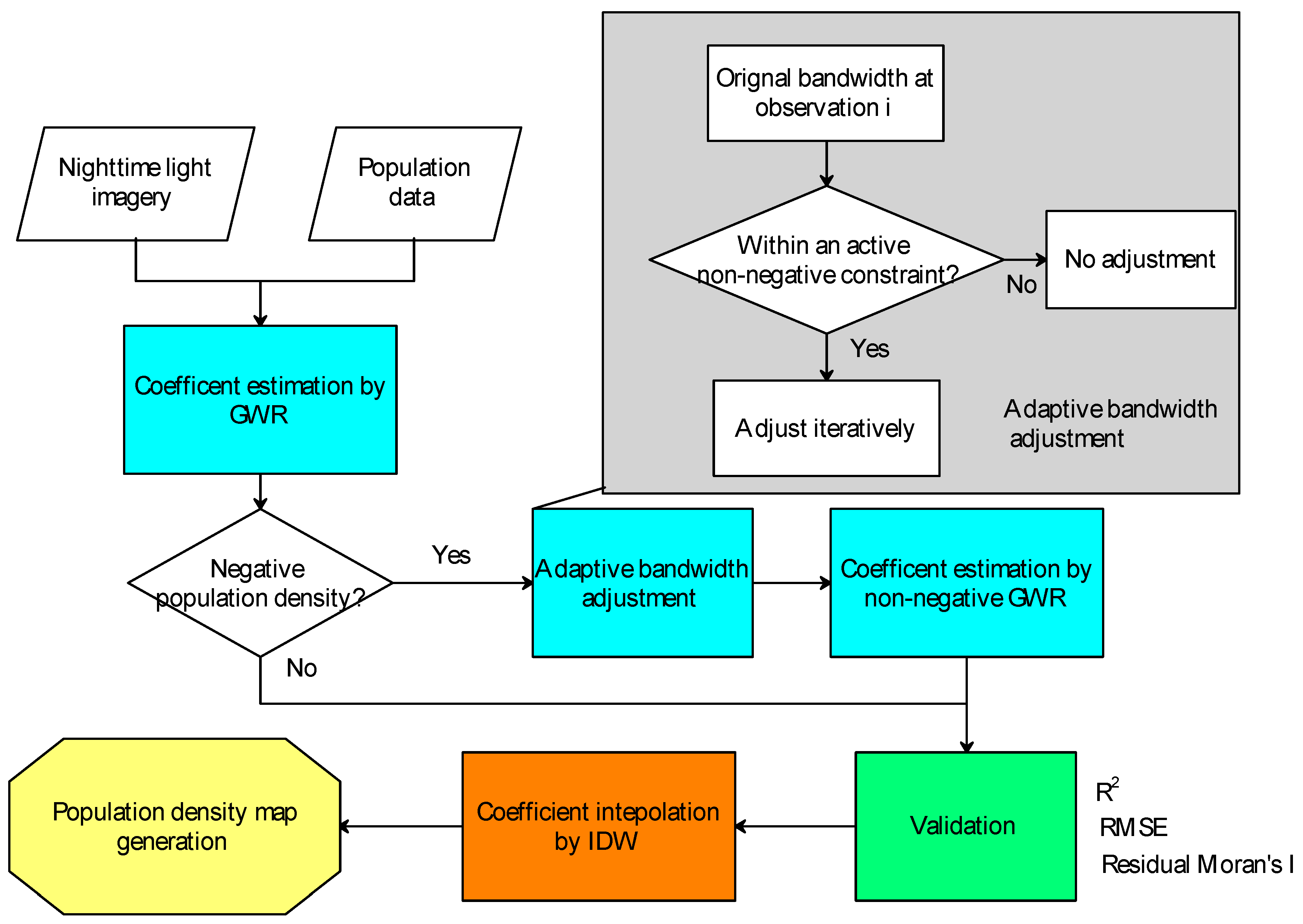
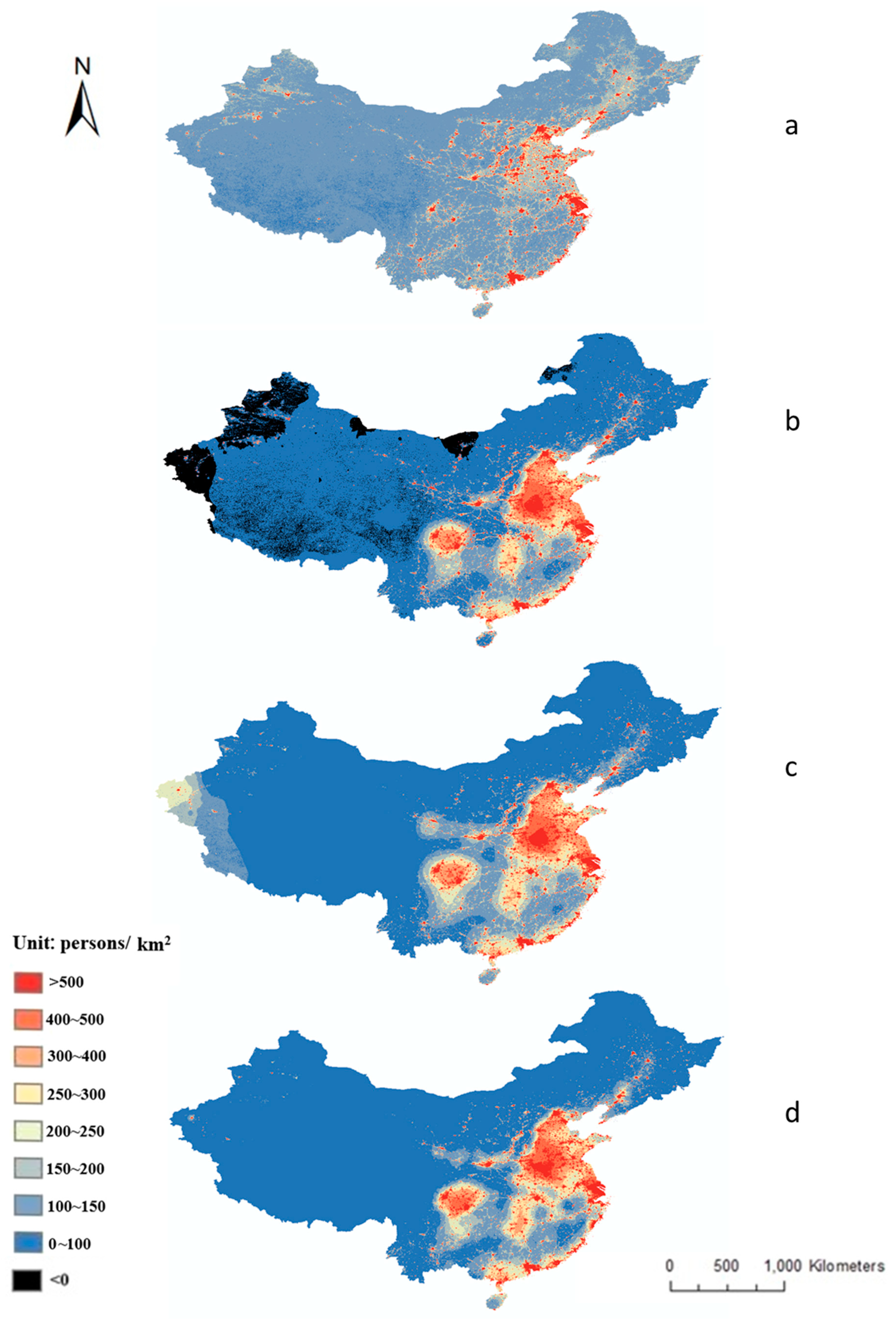
3.1. Model Comparisons among OLS, GWR, NNGWR, and ANNGWR

Table 1 shows the RMSEs of OLS, GWR, NNGWR, and ANNGWR. The GWR model outperforms the OLS. The GWR model is more accurate than the OLS model, which does not consider the spatial variation of coefficients. Figure 3 shows the spatial maps of population density in 2007 from the OLS, GWR, NNGWR, and ANNGWR. The OLS overestimates the population density in the rural area (Figure 3a). The GWR model with spatial weighting considers the spatial heterogeneity in the regression model between nighttime lights and population density. The GWR model can estimate the spatial relationship of nighttime lights and population density. The negative population density from GWR is found in the western areas of mainland China, e.g., Xinjiang, Mongolia, Tibet, Qinghai, Gansu, and Sichuan (black color in Figure 3b), where the population density is considerably low. This negative population density in the GWR is unreasonable for interpretation. The GWR is a local regression model for handling spatial heterogeneity of nighttime lights and population density. However, the model easily generates the negative population problem in areas with low population density. The slope coefficient is approximately −50–250 persons/km2/DN, and the intercept is −600–600 persons/km2 in the original GWR. Accordingly, this study further considers the NNGWR model. The slope and intercept coefficients in NNGWR are constrained in 0–180 persons/km2/DN and 0–850 persons/km2, respectively. The RMSE of NNGWR increases slightly compared with GWR (Table 1). Figure 3c shows that the negative population density is improved using the NNGWR. However, the population density is largely overestimated in the western border provinces (Xinjiang and Tibet) using NNGWR.
Previous studies have demonstrated that the spatial autocorrelation of the error term (model residual) in a regression model exists or is not based on global and local Moran’s I [18,19]. The present study provides the values of this index to prove that the GWR, NNGWR, and ANNGWR decrease the spatial autocorrelation of the residual term, i.e., global Moran’s I (Table 1). Global Moran’s I in ANNGWR is close to zero, i.e., the random distribution of the residuals. Figure 4 shows the spatial maps of local Moran’s I coefficients in the four models. The OLS contains a large number of low–low (LL) points, i.e., low residual values and low neighboring ones, in central China and high–high (HH) points in western area. Several LL points are in the central and coastal areas in the GWR, whereas HH points are in the western area in the NNGWR. The ANNGWR can obtain the best results, e.g., low spatial autocorrelation of the residual term. The ANNGWR has more unsubstantial points than the other models, thereby implying the random distribution of residuals in ANNGWR. The ANNGWR effectively considers spatial relations for the spatial heterogeneity in the regression model.

3.2. ANNGWR Details

Figure 5 shows the simulation and observation in the OLS, GWR, NNGWR, and ANNGWR models. The R2 of OLS is only 0.45 (Figure 5a). The ANNGWR is the best model (Figure 5d) without negative values of population density and serious overestimation problems. In the ANNGWR, the kernel bandwidth is adaptive for effective coefficient estimation, if the coefficients are only allowed to be positive. The bandwidth strikes a balance between precision improvement and smoothness by focusing on observations [20]. On the basis of the iterative approach, the suitable bandwidth is modified to 0.01. Figure 6 shows the population density maps of ANNGWR from various bandwidths in 2007. As the bandwidths increase, overestimation of the population density in the western area of mainland China becomes more serious. The population density overestimation can be solved by considering a small bandwidth of nonnegative coefficient estimation. Figure 7a shows the best (nonnegative and without overestimation) spatial maps of population density in ANNGWR. The RMSE and Moran’s I of ANNGWR show the best performance (Table 1).
Figure 7 shows the ANNGWR model coefficient maps (intercept and slope) in 2007. The spatial model coefficients imply that the ANNGWR can estimate the spatial relationships between the nighttime light and population density. The high values of intercept exist in the city area, if local residents do not rely on lights; by contrast, the low values are in the rural area. In addition, the slope values are higher in the east-southern area than in the western rural area. Nighttime light and population may present a weak relationship in rural areas where electric power infrastructure is unpopular.

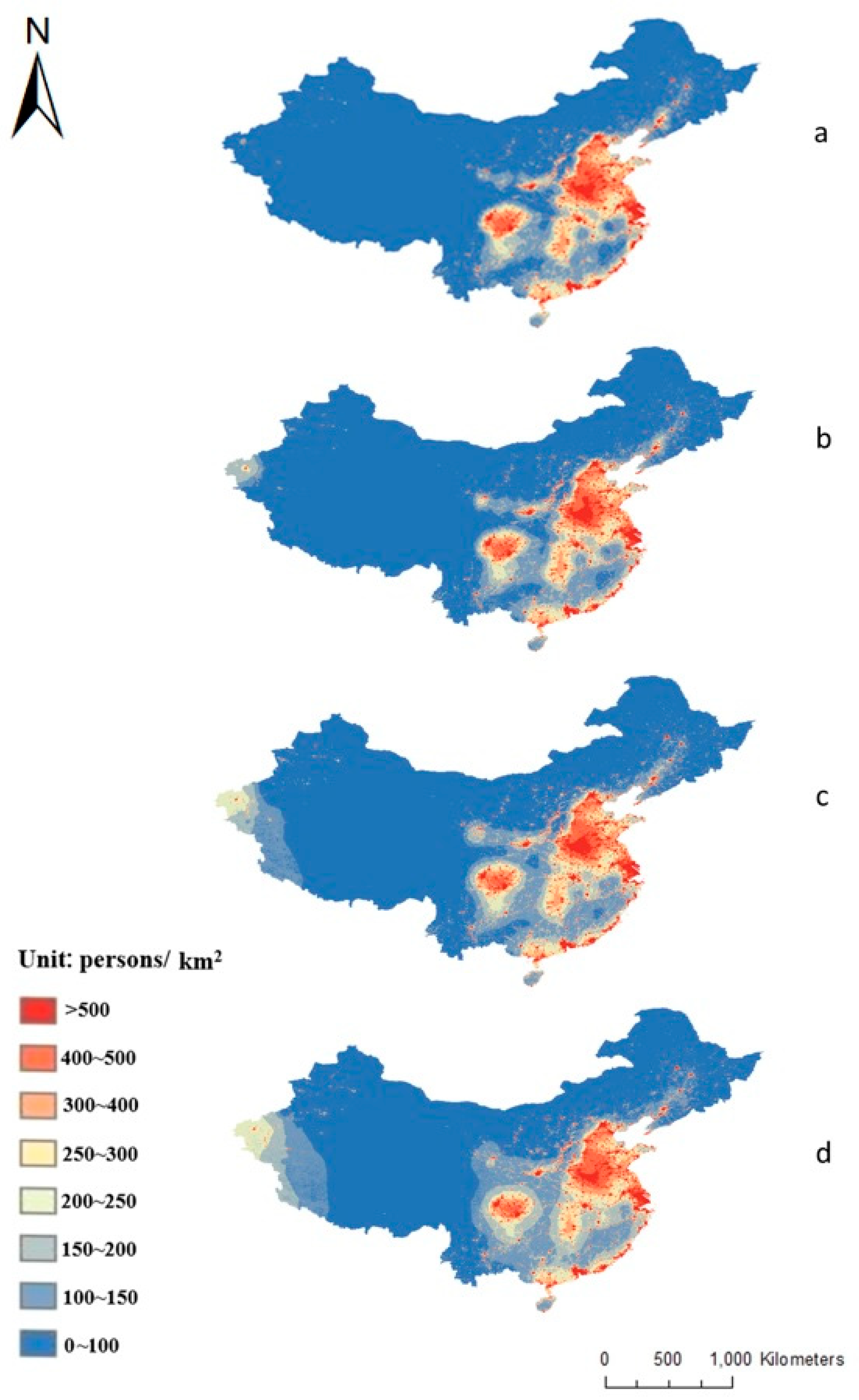
3.3. Temporal Population Density Maps

By considering multiple years’ nighttime images, the details of population change and the pattern of urbanization can be easily traced using the developed method in the present study. Figure 8 shows the simulation of the population density in 2004, 2007, 2010, and 2013. The figure displays the distribution, shape, and compactness of urban growth over the last decades. Population density, e.g., in areas surrounding the Beijing city and in the Hebei province, has increased remarkably across the years. These results are useful for social scientists in studying the changing patterns of urbanization within a given county and across different localities. For urban planners, efficient and sustainable urban designs are easily developed on the basis of the prediction generated by the ANNGWR. These tasks can hardly be achieved by examining the traditional population data because the annual survey of population number only reports aggregate data at the county level and does not reflect the detailed spatial differences within a given county. Figure 8 shows that the spatial population density from nighttime light images correctly reflects the huge population disparity between the eastern and western areas in mainland China. Hence, the nighttime light images can successfully explain the current population density patterns on the basis of our model. The maps prove that the most crowded coastal areas of mainland China are near the Yellow, Yangtze, and Pearl Rivers. As shown in the Chinese population density maps, most people are concentrated in large cities, e.g., Shanghai, Beijing, Tianjin, Shenzhen, and Guangzhou. This finding echoes the findings of Lo [10], where the urbanization of large cities in mainland China can be defined from the nighttime light images. Moreover, the urban expansion near the Yangtze River occurred at an increasing rate until 2007 [21].
In future research, urban and rural areas should be clustered and modeled to increase the model performance. In this manner, regional difference between urban and rural areas can be considered using land use data, nighttime light imagery, and optimization algorithm [4,22]. Future research can also use nighttime light data with the DN calibration process to characterize urbanization dynamics [23,24].

4. Conclusions

This study proposes a population density mapping scheme solely on the basis of nighttime light images and population survey data and offers an effective approach for exploring the spatial patterns of regional population density using ANNGWR. The GWR model is a spatial regression method and is useful in identifying spatially varying regression coefficients between the remote sensing and survey data. However, this model easily identifies meaningless negative population density in rural areas on the basis of nighttime light data. The ANNGWR solves the negative value of population density and serious overestimation problem from GWR. With this setting, the model provides further details on the space variations of population. The ANNGWR has the best goodness-of-fit and lowest Moran’s I coefficient compared with OLS and GWR. This model offers a robust approach for estimating the spatial patterns of population density in mainland China.
In a nutshell, our findings contribute to the study of the spatiotemporal patterns of urbanization in developing countries. After correcting the problems of meaningless negative values and overestimation, the results can help predict population density. We can analyze the detailed urbanization process within a given local area and across different years. Furthermore, our study helps handle the missing values in several government-released population records. As mentioned, in numerous developing countries, the government may influence the release of data, thereby leading to missing records. Our estimation provides a reasonable correction of this problem. In addition, other factors correlating with population density, such as landform and land cover, should be further considered in future research.

Author Contributions

H.-J.C. contributed to model formulation, study design, data preparation, data interpretation, and the writing of the manuscript. C.-H.Y. contributed to data analysis and the reporting of results. C.C.C. contributed to data processing and the writing of the draft manuscript. All authors have seen and approved the final version.

Funding

The APC was funded by MOST (107-2410-H-002-146-MY2 and 107-2622-M-006-001-CC2).

Acknowledgments

The authors thank Teng for his valuable comments and suggestions.

Conflicts of Interest

The authors declare no conflict of interest.

References

  1. Sutton, P. Modeling population density with night-time satellite imagery and GIS. Comput. Environ. Urban Syst. 1997, 21, 227–244. [Google Scholar] [CrossRef]
  2. Mellander, C.; Lobo, J.; Stolarick, K.; Matheson, Z. Night-time light data: A good proxy measure for economic activity? PLoS ONE 2015, 10, e0139779. [Google Scholar] [CrossRef] [PubMed]
  3. Li, Q.; Lu, L.; Weng, Q.; Xie, Y.; Guo, H. Monitoring urban dynamics in the southeast USA using time-series DMSP/OLS nightlight imagery. Remote Sens. 2016, 8, 578. [Google Scholar] [CrossRef]
  4. Sun, W.; Zhang, X.; Wang, N.; Cen, Y. Estimating population density using DMSP-OLS night-time imagery and land cover data. Analysis 2017, 8, 60. [Google Scholar] [CrossRef]
  5. Rayner, P.J.; Raupach, M.R.; Paget, M.; Peylin, P.; Koffi, E. A new global gridded data set of CO2 emissions from fossil fuel combustion: Methodology and evaluation. J. Geophys. Res. Atmos. 2010, 115. [Google Scholar] [CrossRef]
  6. Gillespie, T.W.; Frankenberg, E.; Fung Chum, K.; Thomas, D. Night-time lights time series of tsunami damage, recovery, and economic metrics in Sumatra, Indonesia. Remote Sens. Lett. 2014, 5, 286–294. [Google Scholar] [CrossRef] [PubMed] [Green Version]
  7. Elvidge, C.D.; Baugh, K.E.; Kihn, E.A.; Kroehl, H.W.; Davis, E.R. Mapping city lights with nighttime data from the DMSP Operational Linescan System. Photogramm. Eng. Remote Sens. 1997, 63, 727–734. [Google Scholar]
  8. Fan, C.C. Population Change and Regional Development in China: Insights Based on the 2000 Census. Eurasian Geogr. Econ. 2002, 43, 425–442. [Google Scholar] [CrossRef]
  9. Bustos, M.F.A.; Hall, O.; Andersson, M. Nighttime lights and population changes in Europe 1992–2012. Ambio 2015, 44, 653–665. [Google Scholar] [CrossRef] [PubMed] [Green Version]
  10. Lo, C.P. Modeling the population of China using DMSP operational linescan system nighttime data. Photogramm. Eng. Remote Sens. 2001, 67, 1037–1047. [Google Scholar]
  11. Fotheringham, A.S.; Brunsdon, C.; Charlton, M. Geographically Weighted Regression: The Analysis of Spatially Varying Relationships; John Wiley & Sons: Hoboken, NJ, USA, 2003. [Google Scholar]
  12. Li, L.; Lu, D. Mapping population density distribution at multiple scales in Zhejiang Province using Landsat Thematic Mapper and census data. Int. J. Remote Sens. 2016, 37, 4243–4260. [Google Scholar] [CrossRef]
  13. National Bureau of Statistics of China. China Statistical Yearbook for Regional Economy 2008–2014 (Zhongguo Quyu Jingji Tongji Nianjian 2008–2014); National Bureau of Statistics of China: Beijing, China, 2009–2015.
  14. Howden, D.; Zhou, Y. Why Did China’s Population Grow So Quickly? Indep. Rev. 2015, 20, 227–248. [Google Scholar]
  15. Chu, H.J.; Huang, B.; Lin, C.Y. Modeling the spatio-temporal heterogeneity in the PM10–PM2.5 relationship. Atmos. Environ. 2015, 102, 176–182. [Google Scholar] [CrossRef]
  16. Lawson, C.L.; Hanson, R.J. Solving Least Squares Problems; SIAM: Philadelphia, PA, USA, 1995. [Google Scholar]
  17. Anselin, L. Local indicators of spatial association—LISA. Geogr. Anal. 1995, 27, 93–115. [Google Scholar] [CrossRef]
  18. Tu, J.; Xia, Z.G. Examining spatially varying relationships between land use and water quality using geographically weighted regression I: Model design and evaluation. Sci. Total Environ. 2008, 407, 358–378. [Google Scholar] [CrossRef] [PubMed]
  19. Chu, H.J. Assessing the relationships between elevation and extreme precipitation with various durations in southern Taiwan using spatial regression models. Hydrol. Process. 2012, 26, 3174–3181. [Google Scholar] [CrossRef]
  20. Rohlfs, C.; Zahran, M. Optimal Bandwidth Selection for Kernel Regression Using a Fast Grid Search and a GPU. In Proceedings of the 2017 IEEE International Parallel and Distributed Processing Symposium Workshops (IPDPSW), Orlando, FL, USA, 29 May–2 June 2017; pp. 550–556. [Google Scholar]
  21. Tan, M.; Li, X.; Li, S.; Xin, L.; Wang, X.; Li, Q.; Li, W.; Li, Y.; Xiang, W. Modeling population density based on nighttime light images and land use data in China. Appl. Geogr. 2018, 90, 239–247. [Google Scholar] [CrossRef]
  22. Zeng, C.; Zhou, Y.; Wang, S.; Yan, F.; Zhao, Q. Population spatialization in China based on night-time imagery and land use data. Int. J. Remote Sens. 2011, 32, 9599–9620. [Google Scholar] [CrossRef]
  23. Lu, H.; Zhang, M.; Sun, W.; Li, W. Expansion Analysis of Yangtze River Delta Urban Agglomeration Using DMSP/OLS Nighttime Light Imagery for 1993 to 2012. ISPRS Int. J. Geo-Inf. 2018, 7, 52. [Google Scholar] [CrossRef]
  24. Kumar, P.; Sajjad, H.; Joshi, P.K.; Elvidge, C.D.; Rehman, S.; Chaudhary, B.S.; Tripathy, B.R.; Singh, J.; Pipal, G. Modeling the luminous intensity of Beijing, China using DMSP-OLS night-time lights series data for estimating population density. Phys. Chem. Earth Parts A/B/C 2018. [Google Scholar] [CrossRef]
Figure 1. (a) County center locations and (b) values of observed population data in mainland China at the county level in 2007.
Ijgi 08 00026 g001
Figure 2. Flowchart of ANNGWR in the study.
Ijgi 08 00026 g002
Figure 3. Population density estimation based on (a) OLS, (b) GWR, (c) NNGWR, and (d) ANNGWR in 2007 (black color: negative population density).
Ijgi 08 00026 g003
Figure 4. Spatial maps of local Moran’s I coefficient based on (a) OLS, (b) GWR, (c) NNGWR, and (d) ANNGWR in 2007.
Ijgi 08 00026 g004
Figure 5. Simulation and observation population density plots from (a) OLS, (b) GWR, (c) NNGWR, and (d) ANNGWR in 2007.
Ijgi 08 00026 g005
Figure 6. Bandwidth adjustment iteratively in ANNGWR, e.g., the bandwidths are (a) 0.01, (b) 0.05, (c) 0.1, and (d) 0.2.
Ijgi 08 00026 g006
Figure 7. Spatial maps of (a) intercept and (b) slope coefficients in ANNGWR in 2007.
Ijgi 08 00026 g007
Figure 8. Estimated population density maps in (a) 2004, (b) 2007, (c) 2010, and (d) 2013 using ANNGWR.
Ijgi 08 00026 g008
Table 1. Model performance of the four models: (a) OLS, (b) GWR, (c) NNGWR, and (d) ANNGWR.
TimeModelRMSE (Persons/km2)R2Global Moran’s I of Model Residuals
2004OLS156.40.350.4381
GWR61.90.900.0106
NNGWR67.70.880.0267
ANNGWR50.20.930.0087
2007OLS155.30.450.0501
GWR68.20.900.0417
NNGWR72.50.880.0220
ANNGWR56.40.940.0058
2010OLS166.10.330.3537
GWR66.20.910.0027
NNGWR73.10.890.0242
ANNGWR55.70.940.0042
2013OLS164.90.480.3091
GWR64.90.920.0053
NNGWR72.80.890.0316
ANNGWR57.70.940.0050

