Article

Agent-Based Modeling of Taxi Behavior Simulation with Probe Vehicle Data

1
Institute of Industrial Science, The University of Tokyo, 4-6-1, Komaba, Meguro-ku, Tokyo 153-8505, Japan
2
Center for Spatial Information Science, The University of Tokyo, 5-1-5, Kashiwanoha, Kashiwa-shi, Chiba 277-8568, Japan
3
Graduate School of Sciences and Technology for Innovation, Yamaguchi University, 2-16-1, Tokiwadai, Ube, Yamaguchi 755-8611, Japan
*
Author to whom correspondence should be addressed.
ISPRS Int. J. Geo-Inf. 2018, 7(5), 177; https://doi.org/10.3390/ijgi7050177
Submission received: 10 March 2018 / Revised: 3 May 2018 / Accepted: 7 May 2018 / Published: 8 May 2018
(This article belongs to the Special Issue Geospatial Big Data and Urban Studies)

Abstract

:
Taxi behavior is a spatial–temporal dynamic process involving discrete time dependent events, such as customer pick-up, customer drop-off, cruising, and parking. Simulation models, which are a simplification of a real-world system, can help understand the effects of change of such dynamic behavior. In this paper, agent-based modeling and simulation is proposed, that describes the dynamic action of an agent, i.e., taxi, governed by behavior rules and properties, which emulate the taxi behavior. Taxi behavior simulations are fundamentally done for optimizing the service level for both taxi drivers as well as passengers. Moreover, simulation techniques, as such, could be applied to another field of application as well, where obtaining real raw data are somewhat difficult due to privacy issues, such as human mobility data or call detail record data. This paper describes the development of an agent-based simulation model which is based on multiple input parameters (taxi stay point cluster; trip information (origin and destination); taxi demand information; free taxi movement; and network travel time) that were derived from taxi probe GPS data. As such, agent’s parameters were mapped into grid network, and the road network, for which the grid network was used as a base for query/search/retrieval of taxi agent’s parameters, while the actual movement of taxi agents was on the road network with routing and interpolation. The results obtained from the simulated taxi agent data and real taxi data showed a significant level of similarity of different taxi behavior, such as trip generation; trip time; trip distance as well as trip occupancy, based on its distribution. As for efficient data handling, a distributed computing platform for large-scale data was used for extracting taxi agent parameter from the probe data by utilizing both spatial and non-spatial indexing technique.

1. Introduction

Taxi behavior is characterized by the dynamic discrete time dependent events involving customer pick-up, customer drop-off, cruising, and parking within the spatial and temporal domain. Simulation models which are a simplification of a real-world system, can help understand effects of change of such dynamic behavior. In this regard, agent-based simulation and modeling, in which each taxi behaves as an agent, can capture such dynamic behavior through reconstructing complex patterns by decomposing complex systems down to the level of single agents that are administrated by sets of behavior rules [1]. The advantage of agent-based modeling is that, rather than modeling the entire system with a single equation, the entire system is modeled with the collection of autonomous taxi agent with rules governing them, which makes complex individual agent behave more naturally [2]. In this way, agent-based simulation and modeling can highlight the effect of a change in taxi services and its impact to driver’s income profitability through optimizing parameters (number of trips, passenger waiting time) derived from simulation. As an example, what will be the impact on taxi behavior service when the number of agents i.e., taxi is increased to the region of low taxi demand or decreased to the region of high taxi demand. Understanding such causality could help better management of taxi fleets with regards to the operational cost as well as improve taxi driver’s income. Moreover, recently, many big cities, such as London and New York, have plans to adopt electric taxis [3], and understanding discrete taxi behavior through agent-based modeling could help optimize locations for charging stations, which are crucial for such electric vehicles.
As taxis services are operational throughout the city, spatial and temporal information from these vehicles can be an asset for governing different aspects of urban management. Information, as such, could contribute mainly to helping make better decision-making processes at both government and local level. Having said this, the constant advancement of collecting moving trajectory data in space and time has opened up the possibility of a wide range of study in the field of spatial information science [4]. One of the primary technologies for retrieval of information of various traffic data is from stationary equipment, like loop detectors, for automatic vehicle identification. However, they are limited to specific sections of road. On the contrary, a probe car, also known as a probe vehicle or floating car, utilizes the running vehicles to gather various traffic information, and has been an emerging ITS technology for modeling vehicle behavior [5,6,7]. Big cities, like New York and Beijing, have taxis already equipped with GPS sensors that collects spatial and temporal data to a data center to be processed to extract traffic information [8]. The taxi driver mobility intelligence is an essential factor to maximize both profit and reliability within every possible scenario, and the knowledge about the service can be an advantage for the driver [9]. However, to understand such stochastic dynamics of taxi behavior, micro-level simulation models are required, which can be further analyzed for optimization of taxi services by adjusting parameters like demand, supply, or altering dispatching algorithm [10].
In this paper, agent-based modeling and simulation (ABMS) was implemented, for which in recent years, has been seen in many areas of application, such as flow evacuation, traffic, and customer flow management [2]. Agent-based modeling and simulation describes the dynamic action of an entity i.e., taxi agent governed by behavior rule and properties, similar to the work presented in [6,11,12], to emulate the taxi behavior in Bangkok, Thailand.
The contributions of this paper are summarized as follows:
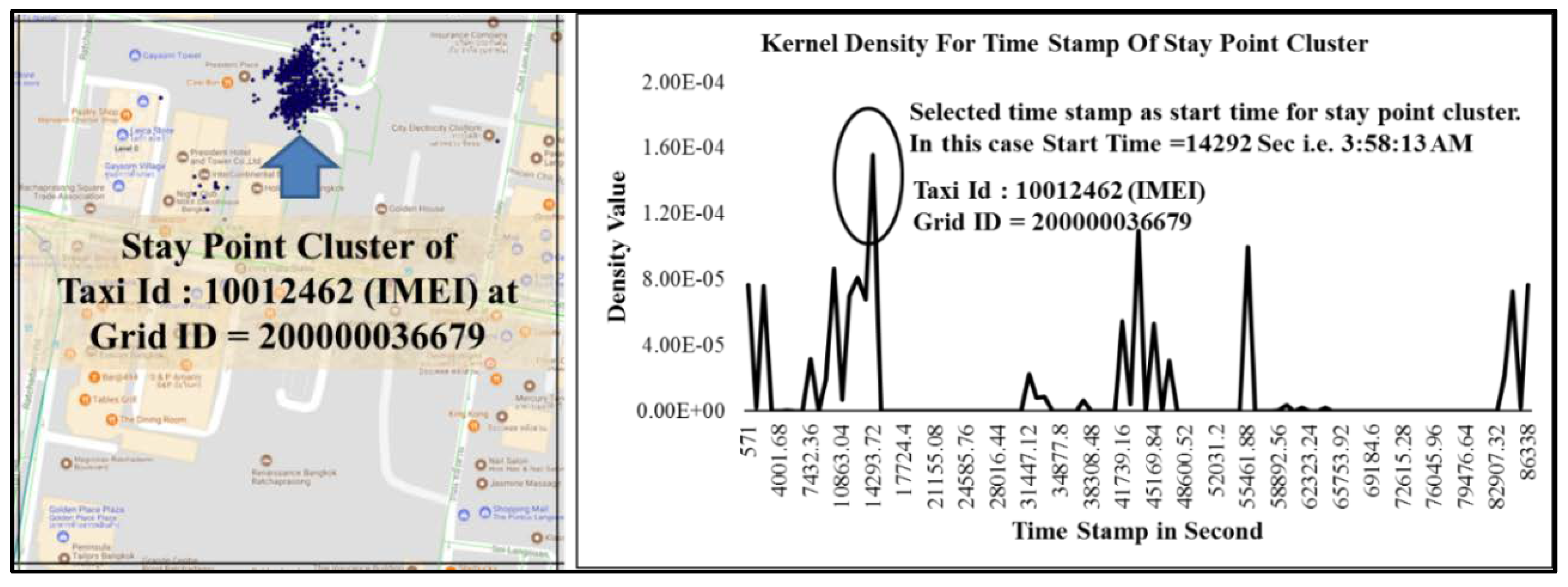
  • Proposed a taxi agent regarding spatial and temporal domain based on a stay point cluster of probe GPS data and a kernel density of its timestamp.
  • Formulated a concept of free taxi movement based on the movement direction of the taxi, which was introduced for searching passengers.
  • Developed an agent-based simulation model which is based on multiple parameters (taxi stay point cluster; trip information (origin and destination); taxi demand information; free taxi movement and network travel time) that were derived from probe GPS taxi data. As such, agent’s parameters were mapped into a grid network and the road network, for which the grid network was used as a base for query/search/retrieval of taxi agent’s parameters, while the actual movement of taxi agents was on the road network, with routing and interpolation.
The motivation of taxi behavior simulation modeling is to optimize taxi service operation, which would be the subject of future study, through an increased number of passenger trips, making drivers wait a less amount of time to get their next passenger, and making more extended passenger trips, as well as determine optimum working time based on the spatial and temporal domain. However, to identifying and evaluating such optimizing parameters, knowing real taxi behavior is a must. The proposed agent-based simulation and modeling recreates the real taxi behavior from which optimizing parameters could be derived, that would improve the taxi service for both driver, regarding monetary profit, as well as for passenger, regarding service level of the taxi.
Also, spatial data, as such, probe GPS taxi data, with its ubiquitous properties, are enormous, and in most cases, deemed confidential. In such cases, obtaining raw spatial data is somewhat complicated. However, simulation and modeling techniques proposed in the study could essentially recreate such spatial data, with secondary data derived, and with properties as similar with the real data. In this regard, such simulation and modeling techniques are not only limited to vehicle behavior, but also could be implemented in simulating human mobility behavior from GPS or call detail record data.

2. Literature Review

In computer modeling, the term “model” describes the abstract or simplified representation of a real world that is already present or planned for the future. The simulation model is typically defined as a mathematical process or an algorithm that depends on various input parameters, which, when processed with mathematical expressions, will result in one or more than one output, encapsulating the behavior and performance of a system in real-world scenarios [11,13].
Taxi service simulation is a dynamic process involving changing demand and supply, as well as urban traffic environment, which suggests stochastic behavior of taxi services that govern the movement, as well as the distribution of taxis [10,14]. Taxi customer bilateral searching and meeting behavior in a network was proposed in [15], which considered stochastic micro-searching behavior of both taxis and customers when they are searching for each other based on customer origin-destination (OD). The model featured location variation in the level of taxi services and stochastic microscopic searching behavior, such that the taxi searched for passenger locally in the network that incorporated Markov chain approach as a route for which transition probability or the link choice probability was specified by the customer pick-up rate within the network. An hourly zone-based origin-destination matrix with the occupied vehicle was developed for evaluating the taxi service behavior, which was then implemented for evaluating time-based taxi demand and supply concerning a given location [7].
A probabilistic based model for time-dependent taxi behavior on a road segment, as well as parking space, was devised for taxi passenger recommendation, in which the probability of picking up a passenger was estimated when the taxi went for a specific parking space [16]. The model was primarily a recommendation system used for suggesting the taxi driver with a location, towards which they would pick up a passenger. Moreover, [17] proposed passenger-finding strategies based on large real-world taxi data which utilized two passenger-finding strategies which were looking or waiting for a passenger that was analyzed using average pick-up number over the given period and location. The model focus was also predicting potential passenger for the event before pick-up and after drop-off only. A time-dependent taxi behaviors model was proposed which incorporated a taxi picking up, dropping off, cruising, and parking system for both taxi drivers and passengers. The model was also primarily a recommendation system that was developed considering the queue length at parking places, along with day type and weather condition. The model provided a number of top parking places along with routes to them, given the current location and time of the taxi driver or a passenger [8].
Time-dependent logit based search models were proposed using global positioning data from an urban taxi, in which profit per unit time was used as the factor characterizing taxi drivers’ search behavior [18]. A cell-based local customer search behavior was implemented for understanding vacant taxi behavior using a cell/grid-based approach which showed customer search decisions were significantly affected by the probability of successfully picking up a customer along the search route [19]. The model was further improved by introducing discrete choice behavior representing taxi search behavior of taxi customers for hailing vacant taxis on the street, proposed by [20], which adopted a multinomial logit approach to model the preference of taxi customers of hailing vacant taxis on streets. Furthermore, the study has been made for a prediction model, which employed learning algorithms to the GPS data. Real-time streaming data was implemented for predicting taxi passenger demand at a given taxi stand [9], in which the model predicted the passenger demand over the taxi stand for a given period in future.
The existing taxi behavior model primarily focuses on finding passenger strategies through demand prediction with a recommendation system, while few studies are present that would provide insight into the effect of an oversupply of taxis in the given area or vice versa [21], the reason for which real taxi behavior modeling is important, as that would replicate the real-world system. The proposed agent-based simulation model in this research primarily focuses on understanding the real taxi behavior by utilizing GPS data from the probe taxi, from which further investigation could be made for an efficient passenger-finding system, managing taxi fleet operations, i.e., optimizing the taxi service operation, as well as understanding the impact of oversupply or undersupply of taxis with respect to existing demand. Agent-based simulation in the field of computational science has proved to become a powerful tool for analyzing complex problems, where random or stochastic behavior, as similar to the taxi behavior, can be presented together with behavioral rules. In this regard, [12] proposed a discrete event simulation model for modeling the behavior of agents operating in a city road network of which agents make their own decisions for making trips. Similarly, [6] further provided a multi-agent-based simulation, which modeled taxi driver’s strategies as a decentralized discrete event, focusing on modeling only the taxi driver’s behavior, which was designed to make an aggregated pattern of taxi movement as similar to the real world.

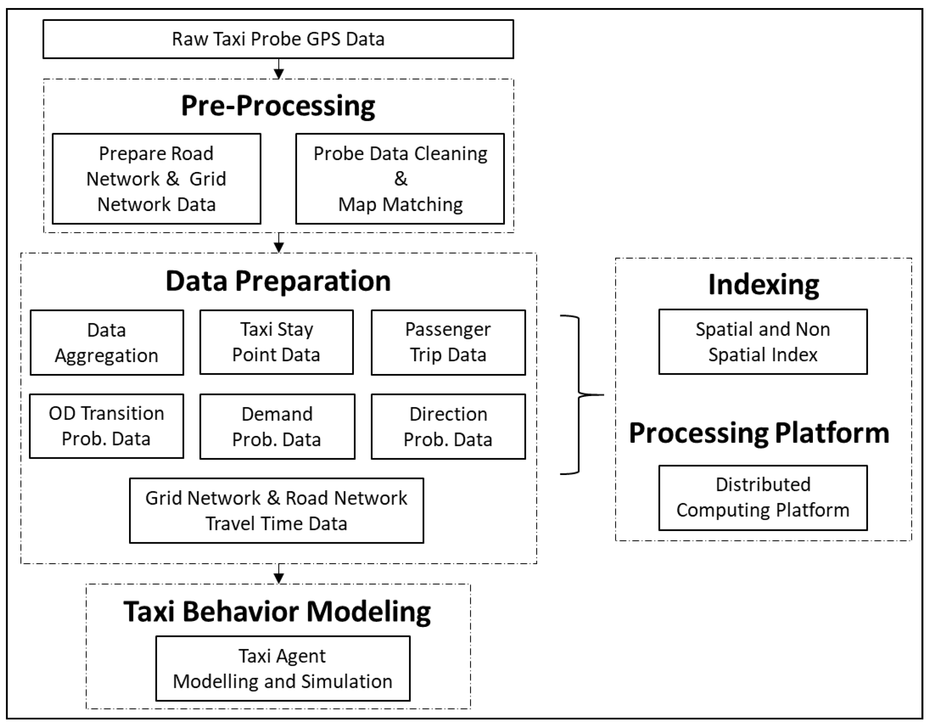
3. System Overview and Preprocessing

The overall system overview is shown in Figure 1, which has preprocessing, data preparation, and taxi behavior modeling as its stages, and indexing and processing platform as its tool to handle the big data. The preprocessing stage consists of preparing for the grid network and road network, with conducting cleaning and map matching of the raw probe GPS data.
In the data preparation stage, multiple secondary datasets from cleaned probe data were extracted, including stay point, passenger trip data, origin-destination probability data, demand probability data, direction probability data, and grid network road network travel time data. In taxi behavior modeling stage, agent-based modeling was implemented, that simulated the taxi behavior of the urban city.
Managing a large volume of data requires an efficient indexing technique that would handle index, search, and retrieval jobs [22]. In this research, both spatial and non-spatial indexing technique was implemented for the simulation purpose. STR tree, which is sort–tile–recursive R tree from Java Topological Suite (JTS), was implemented to index and search spatial data. As for non-spatial data, an index and search engine named Lucene, that works on vector space model algorithms, was implemented for all query, search, and retrieval tasks during the simulating operation [23].
In addition to the large indexing volume of data, the preprocessing of all the data to be utilized for simulation, including cleaning, retrieving trip information, origin-destination, stay point extraction, direction movement extraction, was conducted in Apache Hadoop/Hive large-scale distributed computing system [24]. The total GPS probe data preprocessed from 1 June 2015 to 31 July 2015 was about 2.2 billion data rows which were stored in Hadoop Distributed File System (HDFS). Each data row consisted of a GPS data points with specification as described in Table 1. For spatial data processing, Apache Hive based query HiveQL (Hive Query Language) was developed including Hive UDF (User Defined Function) and Hive UDAF (User Defined Aggregated Function).

3.1. Vehicle Probe Data

In this research, the vehicle is the taxi that is running in and around Bangkok, Thailand, of which data is provided by Toyota Tsusho Nexty Electronics (Thailand) Co., Ltd., Bangkok, Thailand. The probe GPS data was collected from approximately 10,000 taxis with a sampling time of 3 s or 5 s, which was collected from 1 June 2015 to 31 July 2015.
Each of the probe data collected belongs to the spatial trajectory generated by moving taxi in geographical space such that trajectory Ti = {p1, p2, p3, …, pj}, where pj = (xj, yj, tj), such that xj = longitude, yj = latitude, and tj = timestamp. Table 1 shows the data specification and sample data of collected probe data.

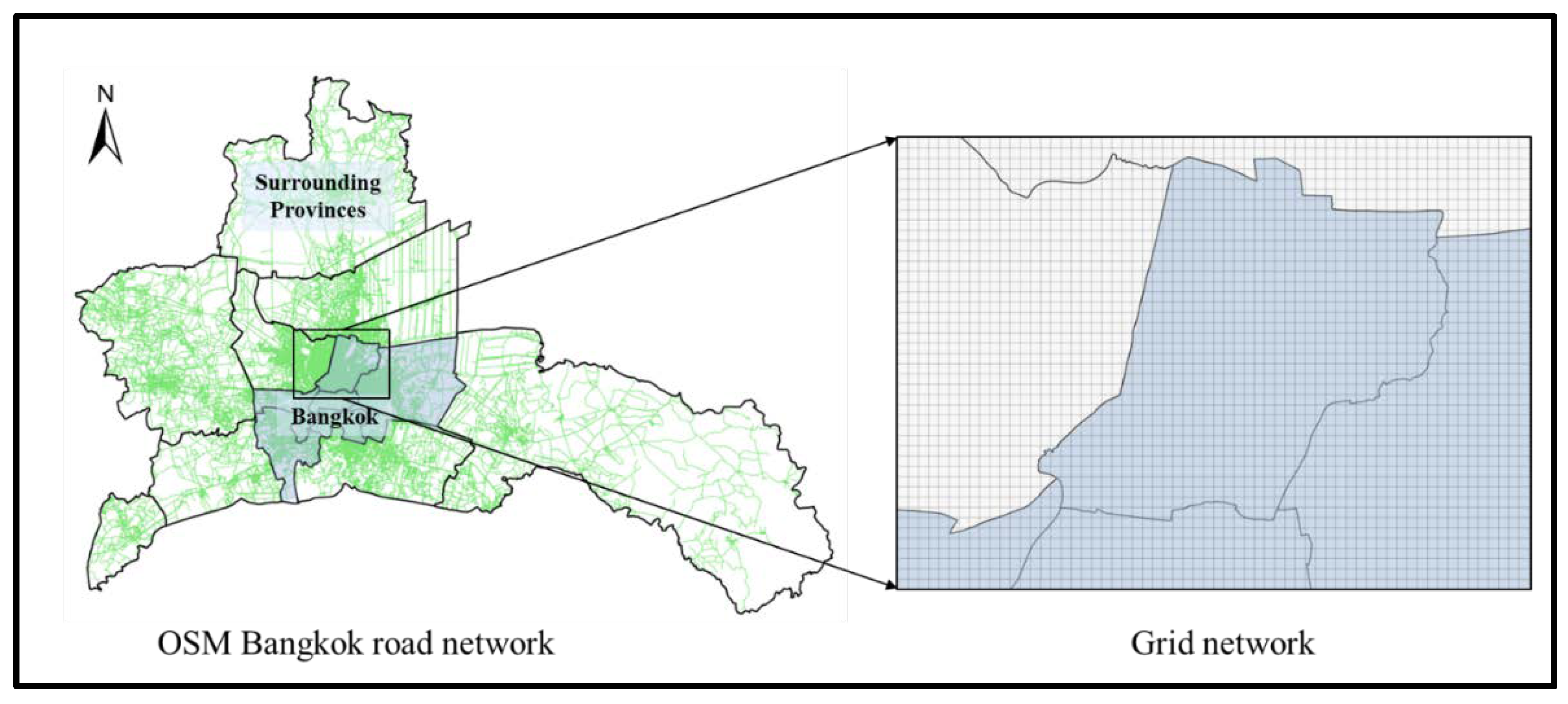
3.2. Prepare Road Network and Grid Network

Open street map data of Thailand was utilized for the road network for which topological error was cleaned [25]. Here, road network was represented by R such that R = {r1, r2, r3, r4, …, rn}, where r1, r2, r3, r4, …, rn is each road segment. The total of 228,416 OSM road network features was extracted for Bangkok and the surrounding provinces. Following the preparation of OSM road network data, taxi probe GPS data were preprocessed to remove erroneous datasets. The cleaned GPS data were then map-matched with probabilistic map-matching process, with open street map road network R [25], that mapped GPS data on the road segment, which was the subject of the previous research work.
The small grid size of 500 × 500 meters was chosen as grid network, in order to preserve spatial patterns and characteristics in the grid [26], however, the optimum grid size selection is still subjective, as larger grid size could be suitable for suburban or rural areas, but not suitable for dense urban area [27]. A grid network of 500 × 500 meters was constructed, covering all of Bangkok region, as well as surrounding provinces. Here, grid network was represented by G such that G = {g1, g2, g3, g4, …, gm}, where g1, g2, g3, g4, …, gm is each grid or cell. The total of 64,620 grid network features was prepared for Bangkok and the surrounding provinces. In addition to the road network map matching, the cleaned GPS data were also mapped to the grid network G. Figure 2 shows the OSM road network and grid network in Bangkok and surrounding provinces.
Grid network was used as it simplified the computation while maintaining both spatial and temporal relevance of the aggregated dataset. Also, use of grid network splits the given spatial region into disjoint areas, which makes it easy to inspect for further qualitative analysis [27]. The road network was used during the preprocessing step of cleaning and map-matching probe taxi data, and then later used routing and interpolation of the simulated taxi agent trajectory, as described in Section 5.

4. Data Preparation

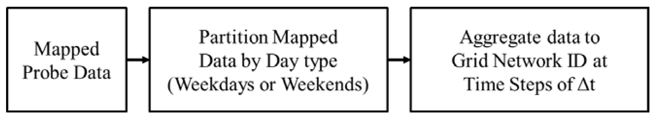
4.1. Data Aggregation

For the grid network mapped data, data were further categorized as weekday and weekend data. Mapped and categorized probe data were then aggregated to each grid network at multiple time steps of 1 h, 15 min, and 5 min. Figure 3 shows grid network G at time steps of Δt.
The flow diagram of a data aggregation process is shown in Figure 4. As mentioned, the probe data were, at first, mapped into the grid network. The mapped data were then partitioned based on weekday and weekend. Finally, an aggregation function was used for aggregating the data for time steps of Δt at road network and grid network for both weekday and weekend data partitioned.

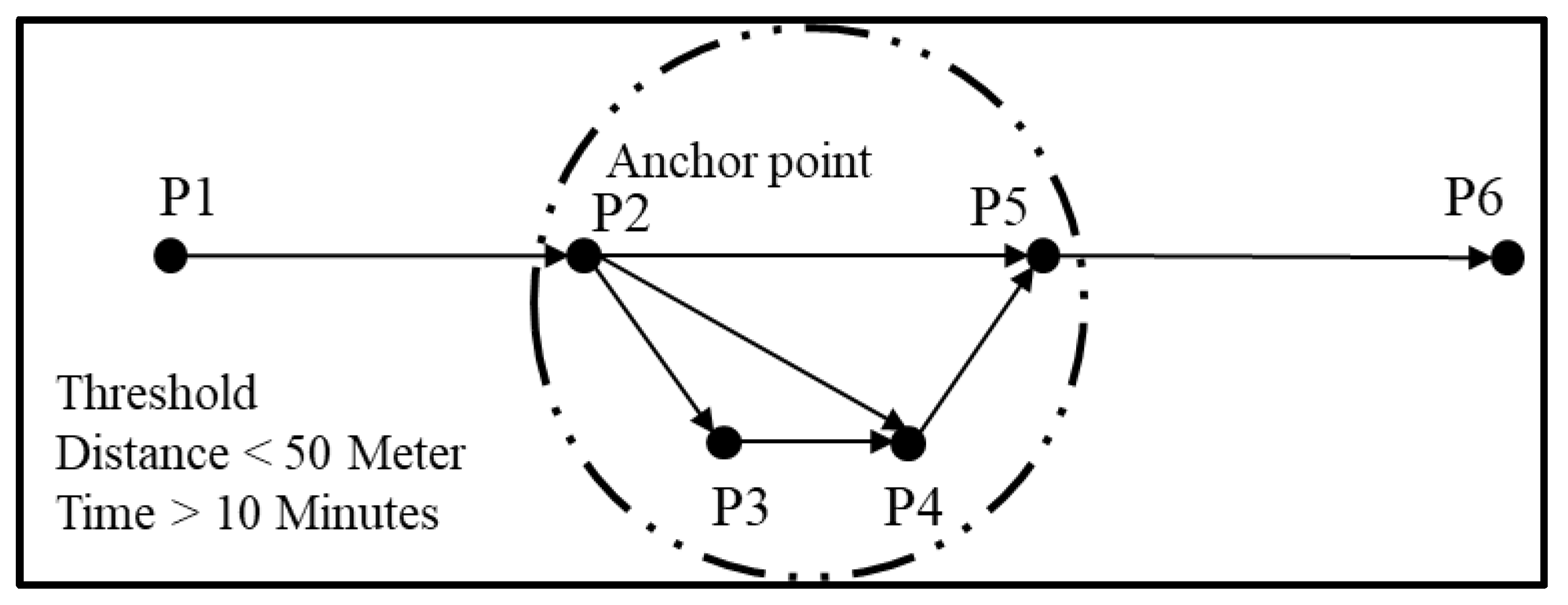
4.2. Stay Point Extraction

Stay point denotes locations where the vehicle (taxi) have stopped or stayed at some location for a certain interval of time, such as a parking place or a gas station, or while looking for a passenger. Taxi stay point cluster location was extracted, which depicts the start location for each taxi during the simulation. The stay point algorithm first checks the distance between the anchor point P a n c h o r P2, as shown in Figure 5, with the successor points P s u c c e s s o r (P3, P4, P5) within the distance threshold D t h r e s h o l d value [28,29]. D t h r e s h o l d was chosen to be 50 meters, which was set empirically. Following this, the time span between anchor point and last successor point P5, which was within the distance threshold, was measured. If the time span measured was greater than the time threshold T t h r e s h o l d value of 10 min, then stay point locations were detected for the given taxi, as shown in Equation (1).
S t a y   p o i n t = { ( P a n c h o r , P s u c c e s s o r ) < D t h r e s h o l d   & ( P a n c h o r , P s u c c e s s o r ) > T t h r e s h o l d
Stay points were extracted for the clustering as to simplify the processing for the clustering algorithm. As mentioned previously, the number of probe GPS data points from probe taxis was about 2.2 billion data rows. Clustering of this vast dataset would take lots of time as well as clusters would be difficult to separate as GPS traces would be dense in particular region. To overcome this difficulty, stay point was extracted that would reduce the computational processing time and would provide meaningful clusters.
A grid G based DBSCAN algorithm was implemented for each taxi stay point identified as proposed in [30,31,32], where the minimum number of points to form clusters (MinPts) and the maximum distance within two points that belongs to the cluster (epsilon ε) were chosen empirically, depending upon the number of clusters required. The MinPts value was chosen as 100 points, and epsilon distance ε was chosen as 50 m. However, both values could be adjusted depending upon the number of clusters required. Improvement on the clustering algorithm could be achieved with HDBSCAN clustering [33] which uses only single parameter, i.e., MinPts for the clustering algorithm. However, as stay points were extracted before clustering, with a threshold distance of 50 m, all those points that were identified as stay points were within 50 m threshold distance. Hence, traditional DBSCAN, with an epsilon distance of 50 m, was used for clustering instead of HDBSCAN. Finally, the centroid of each cluster was computed that represented the stay location for each taxi. For each of the clusters, the start time was computed that represented the starting time for the taxi during simulation, using the kernel density function for the timestamp of each of the points in the clusters. High kernel density value of timestamp was chosen as the start time. The left Figure 6 shows an example for stay point cluster for taxi id “10012462” at grid id “200000036679”. The right Figure 6 shows the kernel density of timestamp all the stay point cluster for taxi id “10012462” at grid id “200000036679”. For this case, the density at timestamp “14,292 s” (3:58:13 a.m.) was the highest, and hence, start time for this taxi was chosen at 3:58:13 a.m. and the cluster centroid as the starting location.

4.3. Taxi Origin and Destination

Taxi origin and destination or OD refer to the location where the taxi picked up and dropped off the passenger or customer [34]. The OD of the taxi was extracted from the taxi trip information, which is tracked through taxi “meter status” of probe data, as described in Table 1. As for the trip itself, only those trips were considered whose origin and destination was within Bangkok and the surrounding provinces, as shown in Figure 2. This also suggested that longer trip information was eliminated and simulation focused more on Bangkok region. Figure 7 shows the passenger trip based on pick-up and drop-off transition.
Meter status transition from 0 to 1 was considered as the start of a passenger trip, and transition from 1 to 0 was considered as the start of the non-passenger trip. Each of the transition locations were mapped onto the grid network G, along with trip distance and trip time computed. A total of 3,081,230 passenger trips and a total of 2,570,432 non-passenger trips were recorded for June and July 2015. Table 2 shows the passenger and non-passenger trip examples for taxi id: 10012462 on weekday.
Based on passenger trip data, an OD matrix was established for a time step of 1 h, for which pick-up location (origin) and drop-off location (destination) pairs were aggregated, based on each grid network G = {g1, g2, g3, g4, …, gm}.
As mentioned previously, there were about 30 million passenger trips recorded for a 2 month period, hence there are about 500,000 OD matrixes derived for each individual day, approximately. The OD matrix of this scale could be easily matched to the closest OSM road network. Doing so, however, generated issues where many OD pairs became sparse, with only one transition between origin and destination road network segment at the given time interval, as shown in Figure 8. Figure 8A shows the case when the OD became sparse, with only one transition between origin road segment and destination road segment, when created using OSM road networks as compared to when created with the grid network, which had 10 transitions between origin grid and destination grid, at the given time interval. Figure 8B shows the pick-up location at the origin with respect to the OSM road network. Similarly, Figure 8C shows the drop-off locations at the destination with respect to the OSM road network. Here, each OD pair corresponding to road network were at different segments, hence creating the sparseness in the OD matrix. Using grid network helped reduce the sparsity problem when creating the OD matrix. In the case when a longer period dataset or larger numbers of taxi data were available, using road network becomes a better option than using the grid network. Other advantages of an OD matrix based in grid is that it could help anonymize the data where data are sensitive, and privacy needs to be protected as well as; such an OD matrix could be applied for understanding interzonal or intercity mobility as well [35]. With the origin-destination matrix for passenger trip, OD transition probability was computed for both weekday and weekend data as shown in Equation (2), which was to be used for passenger trip simulation, as described in Section 5.
g G t , P ( g O D ) = T r i p O D T r i p O
where P ( g O D ) is the OD probability for all grids g that belongs to G at time interval t , such that T r i p O D is the total number of passenger trips between the origin grid O and the destination grid D , and T r i p O is all the passenger trips that originated at grid O at time interval t . The concept behind the use of conditional probability of the OD matrix as shown in Equation (2) was to construct the transition probability matrix between origin and the potential destinations, such that for any given passenger trip generated during simulation, taxis at the origin would move to the destination estimated by the OD transition probability matrix for the given time interval. The OD probability transition matrix, however, could be the subject of periodic update [36] at specific time intervals as agents start to move along the spatiotemporal domain, which could provide the indirect interaction between the agents during the simulation process. Figure 9 shows the passenger trip OD visualization at a time interval of 7 a.m. to 8 a.m., and 18 p.m. to 19 p.m. Each line segment in the OD visualization represented the passenger trip from origin grid O to destination grid D , while the width of the line segment represented the number of trips. The higher the number of trips, the broader was the line segment, and vice versa.

4.4. Taxi Demand

Passenger demand for the given time interval was defined as the total number of passenger pick-ups within the given spatial region. In general, demand is the passenger pick-up count in the spatial and temporal domain [16,19,37,38]. Demand for a taxi was computed with the concept of probability of success or probability of finding passenger, as proposed by [19,39], which was the demand that generated in the grid over the number of vacant taxis in that grid in that given time interval for both weekday and weekend data, as shown in Equation (3).
g G t , P ( d m ) g = O g V g
where P ( d m ) g is the probability of success for all grid g G at time interval t , such that O g and V g are the total number of demands generated and total number of recorded vacant taxis at grid g G and time interval t , respectively. The time interval for demand probability was chosen for every 1 h interval. Figure 10 shows the aggregated demand of taxi in morning hour from 7 a.m. to 8 a.m. and in the evening hour from 18 p.m. to 19 p.m.
The passenger demand for each grid and each time interval varies as shown in Figure 10, which also implies that the probability of success varies accordingly. This indicated that the probability of success was subject to spatial and temporal variation, which could be captured through demand estimation. However, different levels of demand-related information (such as conservative, empirical, informed in real time, and informed about predictions) using data-driven Artificial Intelligence (AI) technologies, and how the information is shared among the driver, could alter and improve the overall behavior and needs to be defined carefully for better demand estimation [40].

4.5. Vacant Taxi Movement

When the taxi has no passenger, the taxi has a total of nine possible cardinal directions to move for searching the passenger, including north (337.5–22.5°), northeast (22.5–67.5°), east (67.5–112.5°), southeast (112.5–157.5°), south (157.5–202.5°), southwest (202.5–247.5°), west (247.5–292.5°), northwest (292.5–337.5°), or stay at the same location. Figure 11 illustrated the nine possible cardinal directions for vacant taxi movement. Based on this assumption, vacant taxi movement was directed for searching of a passenger, with a directional probability which was estimated for both weekday and weekend data, as shown in Equation (4), for each grid at a time interval of every 5 min.
g G t , P ( d ) g = n g N g
where P ( d ) g is the direction probability for vacant taxi movement, moving to direction d , for all grid g G at time interval t , such that n g and N g are the number of vacant taxi points moving to direction d , and the total number of vacant taxi points in grid g G , and time interval of t , respectively. The direction the vacant taxi would choose for searching for passengers was estimated from the highest P ( d ) g obtained for a given grid and time interval.

4.6. Network Travel Time

GPS probe data now enables us to collect the travel time information through the moving vehicle, and has the given convenience to make travel time predictions in a complicated road network, whereby road network travel time can be estimated by estimating the speed between the nodes of the road segment [41,42]. GPS probe data can essentially provide information of a traffic condition of a given period, such as travel time estimation, as well as traffic congestion, which directly relates to the distance travelled by a vehicle in that period [43]. In this paper, the average road network segment speed and average grid network speed was estimated for the time step of every 15 min time interval for both weekday and weekend data, as shown in Equations (5) and (6). The estimated average road network segment speed and average grid network speed was used for estimating taxi travel time during the simulation movement.
r R t , s ¯ r = S p r N p r
g G t , s ¯ g = S p G N p G
where, s ¯ r and s ¯ g are the average speed on the road network segment r R , and grid network g G , respectively at a time interval of t , such that S p r and S p g are the sum of the speed of all the points p with N p r and N p g as the total number of points belonging to its respective network. The use of two different average speeds was because not all road network segments had the probe GPS point associated with it at a given time interval. In such cases, the road network segment average speed could not be computed. Hence, grid network average speed was used instead for the given road network segment associated with it at the given time interval. In this regard, road network travel time was given by Equation (7).
T r : p ^ t = { r d i s t a n c e s ¯ r r d i s t a n c e s ¯ g
where, T r : p ^ t is the road network travel time with r d i s t a n c e as road network segment distance, such that for any point p ^ that appears on road network segment r R and grid network g G at time interval t during simulation, would require T r : p ^ t unit time to cross or complete the road network segment.

5. Methodology

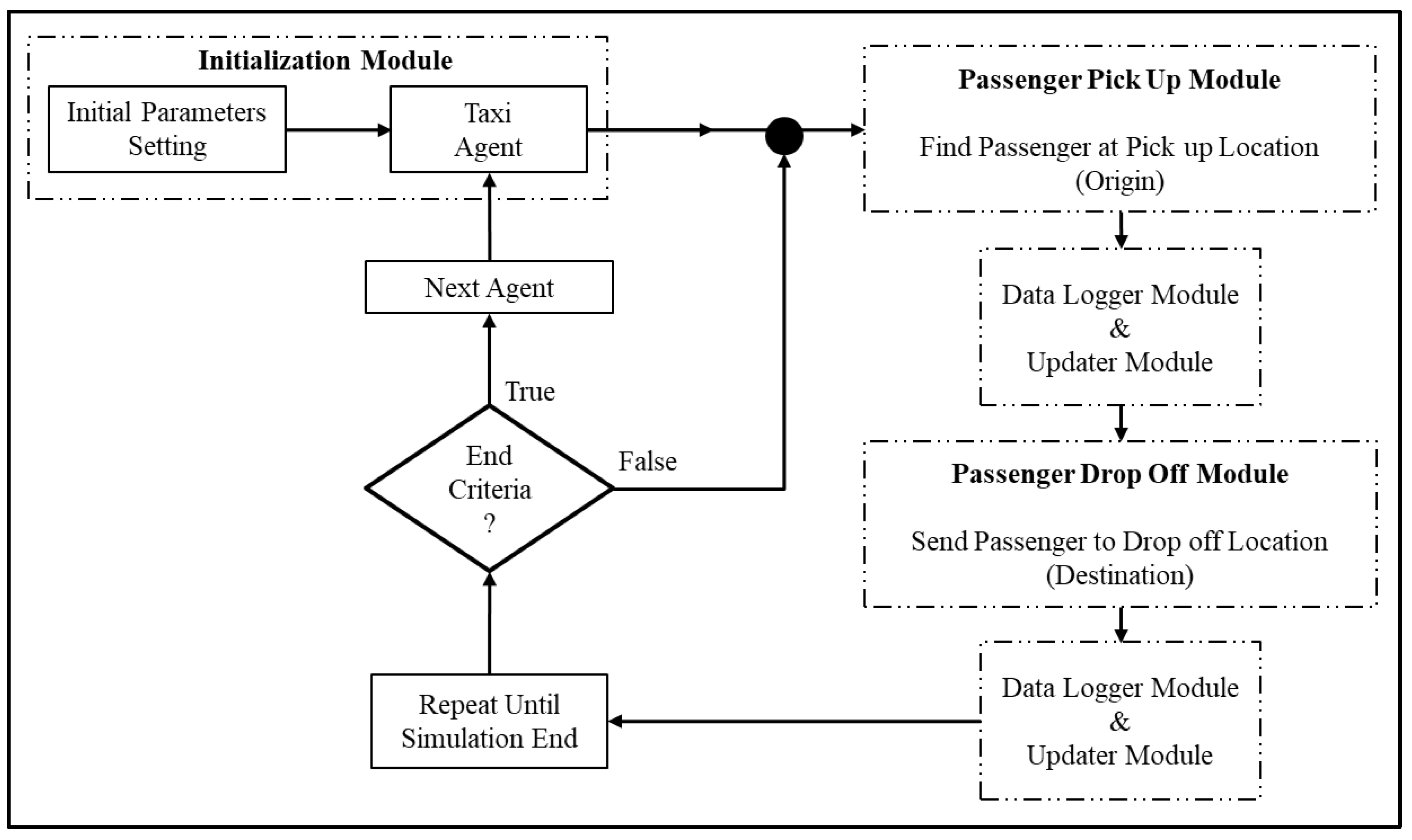
5.1. Agent-Based Model

An agent-based simulation model was designed to simulate the discrete event of real taxi movement as it happens in the real-world situation. The entire model was subdivided into five different submodules which were initialization module, passenger pick-up module, data logger module & updater module, passenger drop-off module, as shown in Figure 12.
In the agent-based simulation model, each taxi was treated as an individual taxi agent, for which they were given a specific behavior rule, based on location and time, for its entire movement. This approach makes modeling flexible, as it makes it easy to add individual variation in the behavior rule, as well as external random influences [44]. The result is an overall characteristic feature of the system from the collective individual entity with rule. Other features that make agent-based simulation promising is the use of modularity, where different events are separated into individual modules.

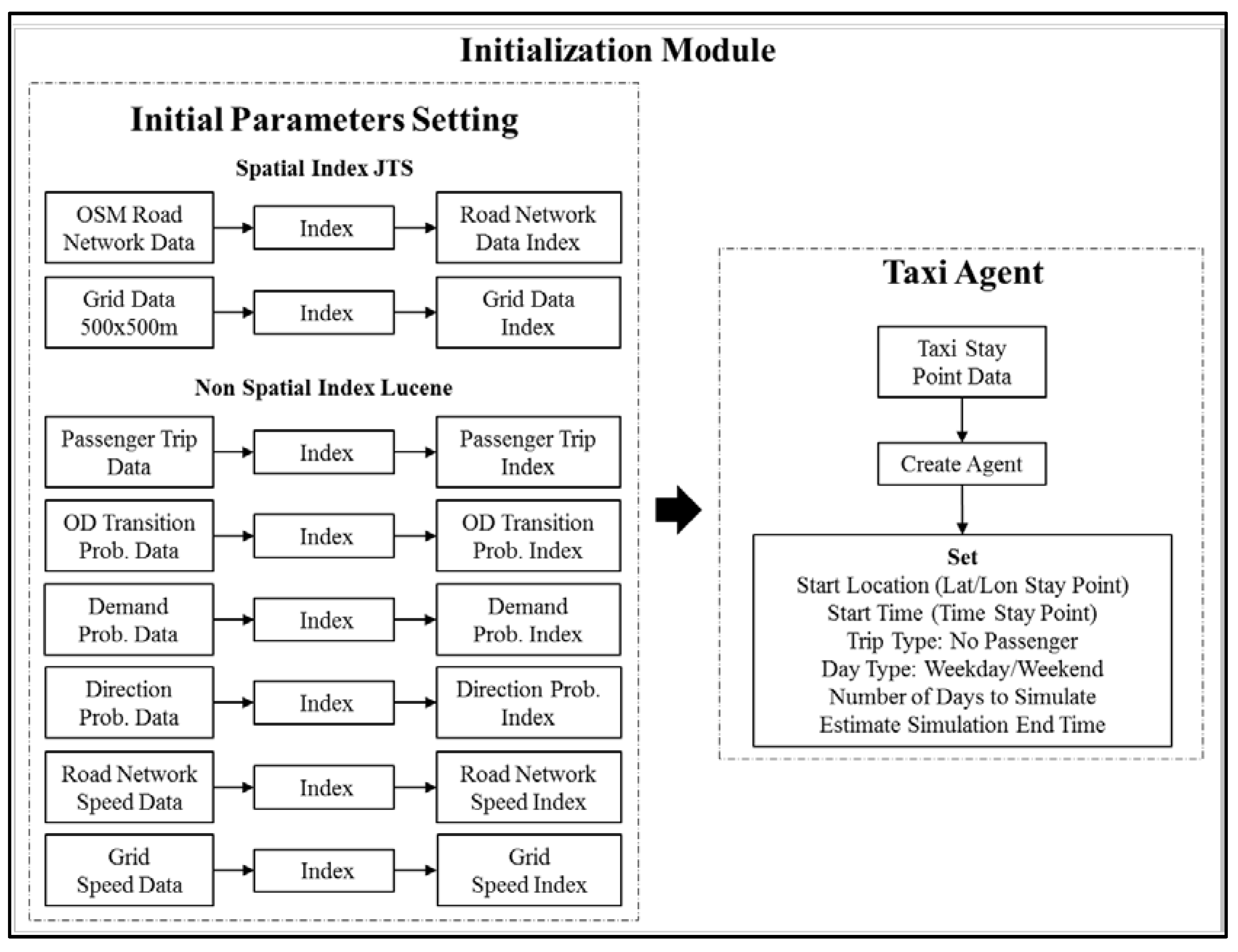
5.2. Initialization Module

In this module, various simulation spatial and non-spatial parameters were indexed. Spatial data parameters included OSM road network and grid network data as described in Section 3.2, whereas non-spatial data parameters included stay point data, passenger trip data, origin-destination probability, demand probability, vacant taxi movement probability (direction probability), OSM road network, and grid network speed data, as described in Section 4. Figure 13 shows the initialization module of the simulation process.

5.3. Taxi Agent

Each of the taxi agents was created based on the taxi stay point cluster extracted from the probe data as described in Section 4.2. For each taxi agent, various parameters were set at the beginning of the simulation, including start location regarding latitude and longitude, start time, trip type, i.e., whether the taxi have a passenger or not, day type, i.e., whether simulation was for weekday or weekend, and some days or hours to run the simulation. Based on taxi agent start time and the number of days or hours for simulation, the end or stop criteria for each taxi agent was determined. As for the starting condition, the assumption was made that the taxi agent will not have any passenger, and hence, after initialization module, the taxi agent would move onto the passenger pick-up module.

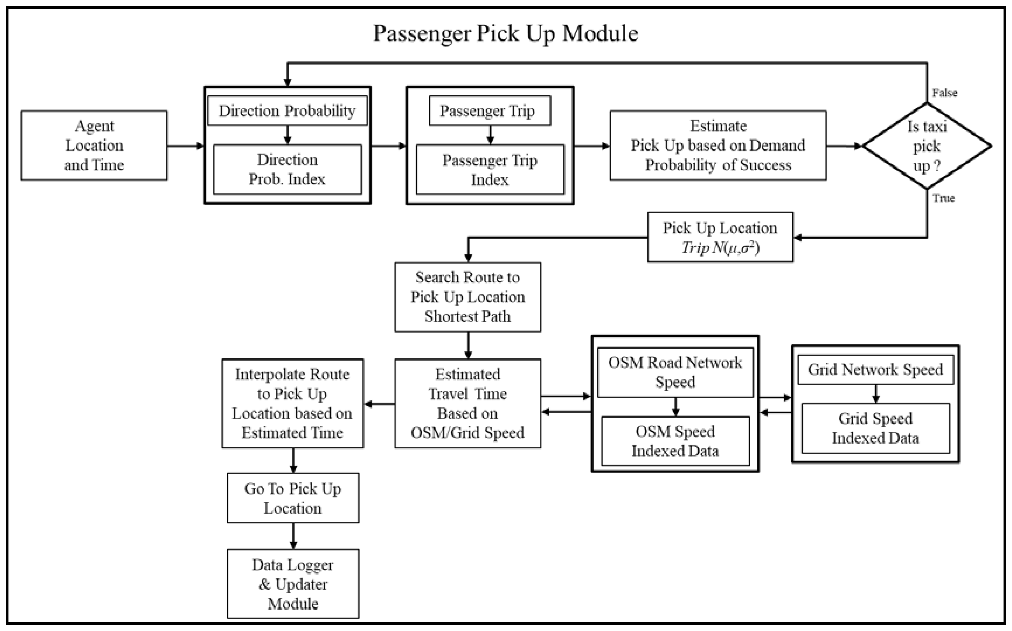
5.4. Passenger Pick-Up Module

In the passenger pick-up module, the taxi agent, based on location and time, would move, searching for a passenger. The searching of the passenger was made based on vacant taxi movement probability or direction probability for the grid that the taxi agent belongs to, and the time interval. Two distinct types of movement could be observed, which were staying in the same grid for searching passenger (taxi queueing event) or move adjoining grid (taxi movement event). For each taxi agent free movement at grid level as described in Section 4.5, an estimation was made as to whether the taxi agent would get a passenger or not, based on demand probability of success, as described in Section 4.4. If there were no pick-up events, then the taxi agent would either stay in the same grid or move to an adjoining grid to look for a passenger. If there was a pick-up event in the grid, then pick-up location was estimated based on the distribution of real passenger trips that had originated in that grid. With pick-up location successfully estimated, the route to the pick-up location was implemented using the Dijkstra algorithm [45] which was based on OSM network. For each road network segment, travel time was estimated and described in Section 4.6. The cumulative travel time of each road segment of the route was then stored as passenger search time. Route interpolation, as described in [46], was then implemented to generate taxi agent points p ^ . to the pick-u location, with the sampling rate of 30 s. The time period was chosen as to maintain the overall trajectory [25] of the taxi agent, along with reducing the data storage load. Data logger module was called in to log all the interpolated points, created during the taxi agent simulation movement, on to the file system. Updater module then resets the parameters for the taxi agent, such as location, as well as time for the succeeding module. Figure 14 shows the detailed passenger pick-up module.

5.5. Passenger Drop-Off Module

Passenger drop-off module subsequently was used for estimating taxi agent drop-off location. Drop-off grid location was estimated based on trip origin-destination probability, as described in Section 4.3, for a given grid as well as a time interval. With drop-off grid estimated, drop-off location was then estimated based on the distribution of real passenger trip that had destinated in that grid. Following, route selection, network travel time estimation, as well as taxi agent route interpolation, was conducted as similar to the passenger pick-up module. Data logger was then called in to log all the interpolated points on to the file system along with updater module to reset parameters for the succeeding module. Figure 15 shows the detailed passenger drop-off module.
For each taxi agent simulation, one iteration cycle was composed of passenger pick-up module, data logger module and updater module, passenger drop-off module, and finally again, data logger module and updater module. Completion of each iteration cycle triggered end criteria condition. If the end criteria as set in initialization module were not met, then the agent would again be moved to passenger pick-up module, and the cycle would continue until the end criteria were met, indicating the end of simulation for a given taxi agent.

5.6. Data Logger and Updater Module

The purpose of the data logger module was to log all the simulated data generated during both passenger pick-up module and passenger drop-off module. Following the data logger module, updater module was called in, as shown in Figure 16. The updater module served mainly two purposes. The first purpose was to update the individual local parameter of an agent, such as agent location and time. The second purpose was to update the global parameters, which included taxi demand probability data, direction probability data, taxi origin destination probability data, and passenger trip data. The global parameter could be updated by merging the simulated data with the real dataset. The new taxi demand probability data, direction probability data, taxi origin destination probability data, and passenger trip data, then could be computed, based on merged simulated and real dataset. The index of the parameters then needs to be updated, which would be used by the agents subsequently during simulation. The update on global parameter provided a mechanism where agent could interact with each other indirectly.

6. Results

The simulation was conducted in two scenarios, i.e., weekday and weekend, each for an entire day, such that overall properties of simulated taxi service behavior within the city was kept intact, as that with the real taxi service, by adjusting various parameters within the simulation process. Various property comparisons, based on distribution, were conducted between the simulated taxi agent data and the real taxi data, that showed the level of similarity between them. The overlapping coefficient, which is defined as a measure of the agreement between two probability distributions [47], was computed to identify the similarity measurement with a scale of 0 to 1. The measured value of 1 indicated a perfect match, while the measured value of 0 indicated no interaction between the distribution. Four different taxi attributes that included trip generated, trip generated per grid, trip time, and trip distance were compared together regarding their distribution, whereas average taxi speed was compared for hourly variation. Finally, occupancy between the simulated and real taxi data was also evaluated.

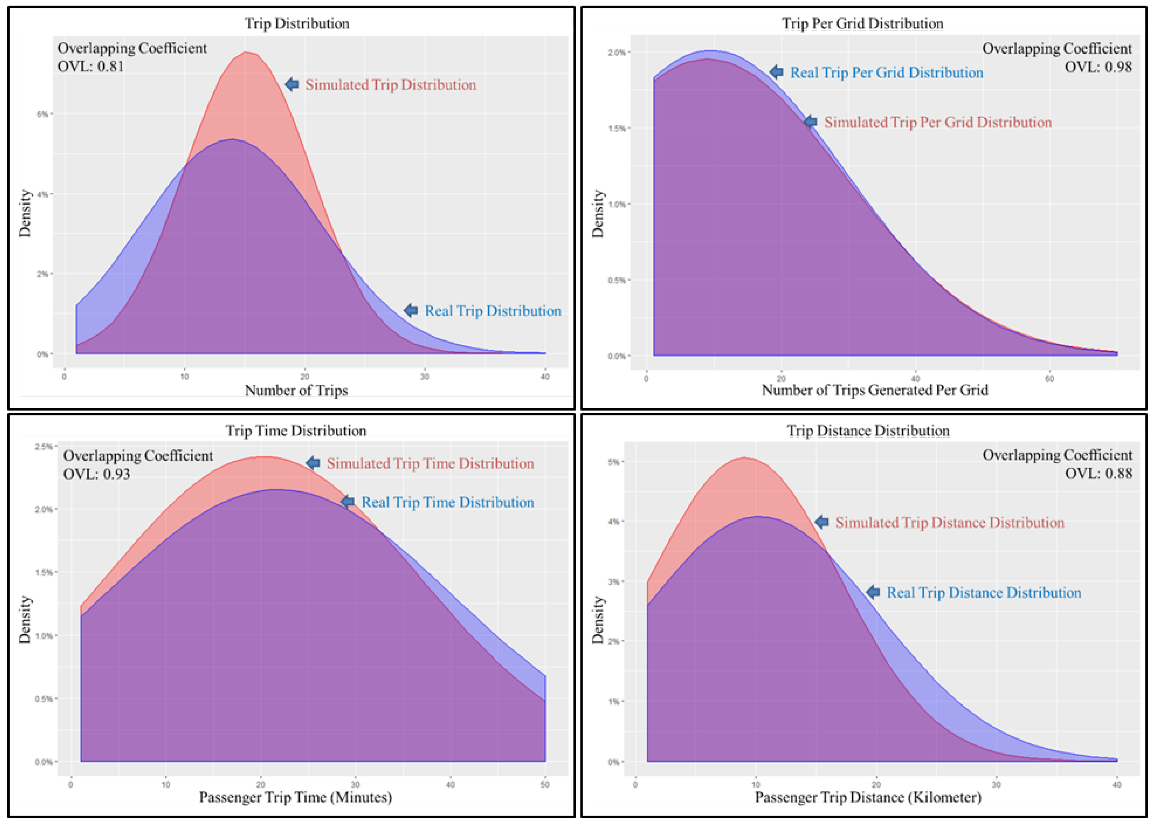
6.1. Distribution Overlapping Coefficient

The weekday’s distribution comparison is shown in Figure 17. Trip distribution comparison between simulated taxi data and real taxi data showed the overlapping coefficient of 0.81, which indicated some trips generated from the simulation were a close match with the real data. Similarly, a number of trips generated per grid distribution showed a very high overlapping coefficient of 0.98, indicating high similarity for the trip generated on the grid level.
As for the trip time distribution, regarding minutes, an overlapping similarity of 0.93 was obtained, which showed significant similarity between simulated trip time and real trip time. Finally, for trip distance, regarding kilometers, a distribution of overlapping similarity of 0.88 was obtained between simulated trip time and real trip time. The significant overlapping similarity for the weekday simulation suggested that the simulated taxi agent emulated the real taxi, keeping overall taxi behavior intact. Table 3 shows distribution properties of the four compared attributes of taxi behavior for the weekday simulation.
The weekend distribution comparison is shown in Figure 18. Trip distribution comparison between simulated taxi data and real taxi data showed the overlapping coefficient of 0.7, which indicated a number of trips generated from the simulation were in accord with the real data. Similarly, a number of trips generated per grid distribution showed a high overlapping coefficient of 0.91, indicating high similarity for trips generated on the grid level.
For trip time distribution, with respect to minutes, the overlapping coefficient of 0.96 was obtained, which showed a significant similarity between simulated trip time and real trip time. Finally, for trip distance distribution, regarding kilometers, an overlapping similarity of 0.86 was obtained between simulated trip time and real trip time. The significant overlapping similarity for the weekend simulation also suggested that the simulated taxi agent emulated the real taxi keeping overall taxi behavior intact. Table 4 shows distribution properties of the four compared attributes of taxi behavior for the weekend simulation.
As described in Section 4.3, only those trips that had origin and destination in Bangkok and surrounding provinces were considered to construct the OD matrix, and subsequently, OD probability. Hence, for both weekday and weekend, in the overlapping coefficient similarity comparison, only those trips within Bangkok and surrounding provinces were considered. Out of all the real passenger trips within Bangkok and surrounding provinces, 97% of the trip had a trip time of less than 2 h, and 98% of the trip had a trip distance less than 100 km. This implies that the simulated result obtained could emulate taxi behaviors for a trip distance within 100 km, and trip time within 2 h.
The simulated data results in parameters i.e., trip count, grid trip generated, passenger trip time (min), and passenger trip distance (km), as compared to the real data result parameters, was marginally lower, as shown in Table 4. However, simulated data result parameters could be maintained by adjusting the demand probability success for which the current threshold value was set empirically to 15%. In addition, the higher value of standard deviation for both simulated weekday and weekend results especially for the grip trip generated and passenger trip time was obtained as the distribution was computed at the grid level for which grip trip generated within the inner city would have obtained more trip as compared to the grid which was located at the outskirts of the city. Similarly, passenger trip time would also vary depending upon the individual trip generated, which resulted in the high standard deviation in simulated result.

6.2. Average Speed Hourly Variation

OSM road network based average speed comparison was conducted for time intervals of 1 h between simulated and real datasets for both weekday and weekend. Figure 19 shows the hourly variation of average speed for the entire region of Bangkok and surrounding provinces. Comparison of an average speed showed an R squared value of 0.96 for the weekday comparison and R squared value of 0.97 for the weekend’s comparison. The high R squared value for both weekday and weekend simulated data suggested simulated taxi agents could keep the real taxi properties intact. As mentioned previously, all query, search, and retrieval tasks were conducted over grid network. However, the routing and route interpolation were conducted over the OSM road network, which is shown in terms of taxi agent trajectory in Figure 20. Similarly, the simulated trajectory for the weekday data at a time interval of every 4 h is shown in Figure 21.

6.3. Taxi Occupancy Evaluation

One of the properties that characterizes taxi service behavior is its occupancy, which is defined as the ratio of taxi driving time with a passenger to total driving time [39]. Figure 22 shows the frequency distribution of taxi occupancy ratio for the simulated taxi agent and real taxi data.
The occupancy ratio analysis showed for simulated taxi agent data occupancy was clustered around 37–41%, whereas for the real taxi data, occupancy ratio was clustered around 48–52%. Though simulated taxi data showed slight underestimation regarding occupancy ratio; the overall distribution was kept similar to the real taxi data.

7. Conclusions

Modeling of taxi service is an important aspect of understanding the behavior of taxi service level in the city. This paper proposes a data driven agent-based simulation model to study simulated taxi behaviors in a large-scale urban area with the taxi probe vehicle data. Analysis of the taxi agent simulation showed a significant similarity with the real taxi data, indicating that the simulated result could keep the real nature of taxi service behavior. The previous study on agent-based modeling for taxi behavior analyses have compared the measured and the modeled travel distance, and travel time with the cost, to validate the model. However, for travel time, results were scattered between the measured and the model data [12], for which two issues regarding road network density and routing were mentioned. In the agent-based modeling presented here, taxi service modeling was categorized based on weekday and weekend. Nevertheless, with the increasing utilization of GPS probe data, modeling of service can be made by adding other entities, such as daily variation, monthly variation, etc. More importantly, such simulation can help understand and predict the effect of having a large number of taxis in the spatial and temporal domain with low demand, and vice versa. Understanding such taxi behavior in the city can significantly help managing and dispatching the fleet of the taxi that can make monetary profit for the drivers.
The limitation of the current agent-based model is that the current agent-based model system utilizes an offline learning method, which possesses constraints in terms of time and resources when required to learn from a high-speed streaming dataset. The offline learning method, despite having many use cases, possess a limitation in regards how it can handle new datasets. In such cases, the model needs to be improved that would help accommodate learning from high-speed steaming data, as proposed in [36], where the OD matrix constantly evolves as time progresses, with the addition of new datasets and removal of the outdated datasets. The model can further be improved in terms of free movement of vacant taxis, with regard to replacing movement directed by direction angle to searching the next road network node at each time interval. Furthermore, current agent-based modeling could describe the taxi behavior with a trip time of 2 h and trip distance of 100 km. Though such trips accounted for about 98% of the total trip, the model could be further improved to encapsulate both short and long trips, regarding both time and distance.

Author Contributions

S.R., A.W. and R.S. conceptualize and designed the system. M.N. and A.W. provided spatial data management framework, technique and methodology. A.W., M.N. and R.S. contributed to the improvement of the overall system and the original manuscript.

Acknowledgments

This research was facilitated and funded by Shibasaki Laboratory (http://shiba.iis.u-tokyo.ac.jp/) of The University of Tokyo. This research was partially supported by Toyota Tsusho Nexty Electronics (Thailand) Co., Ltd., by providing Taxi Probe Data for research purpose. The author would like to thank Hiroshi Kanasugi from The University of Tokyo who provided insight and expertise that greatly assisted the research.

Conflicts of Interest

The authors declare no conflict of interest.

References

  1. Baster, B.; Duda, J.; Maciol, A.; Rebiasz, B. Rule-Based Approach to Human-like Decision Simulating in Agent-Based Modeling and Simulation. In Proceedings of the 2013 17th International Conference on System Theory, Control and Computing (ICSTCC) 2013, Sinaia, Romania, 11–13 October 2013; pp. 739–743. [Google Scholar]
  2. Bonabeau, E. Agent-Based Modeling: Methods and Techniques for Simulating Human Systems. Proc. Natl. Acad. Sci. USA 2002, 99 (Suppl. 3), 7280–7287. [Google Scholar] [CrossRef] [PubMed]
  3. Tu, W.; Li, Q.; Fang, Z.; Shaw, S.-L.; Zhou, B.; Chang, X. Optimizing the Locations of Electric Taxi Charging Stations: A Spatial–temporal Demand Coverage Approach. Transp. Res. Part C Emerg. Technol. 2016, 65, 172–189. [Google Scholar] [CrossRef]
  4. Sadahiro, Y.; Lay, R.; Kobayashi, T. Trajectories of Moving Objects on a Network: Detection of Similarities, Visualization of Relations, and Classification of Trajectories. Trans. GIS 2013, 17, 18–40. [Google Scholar] [CrossRef]
  5. Miwa, T.; Sakai, T.; Morikawa, T. Route Identification and Travel Time Prediction Using Probe-Car Data. Int. J. ITS Res. 2004, 2, 21–28. [Google Scholar]
  6. Cheng, S.F.; Nguyen, T.D. TaxiSim: A Multiagent Simulation Platform for Evaluating Taxi Fleet Operations. In Proceedings of the 2011 IEEE/WIC/ACM International Conferences on Web Intelligence and Intelligent Agent Technology, Lyon, France, 22–27 August 2011; Volume 2, pp. 14–21. [Google Scholar]
  7. Bischoff, J.; Maciejewski, M.; Sohr, A. Analysis of Berlin’s Taxi Services by Exploring GPS Traces. In Proceedings of the 2015 International Conference on Models and Technologies for Intelligent Transportation Systems (MT-ITS), Budapest, Hungary, 3–5 June 2015; pp. 209–215. [Google Scholar]
  8. Yuan, N.J.; Zheng, Y.; Zhang, L.; Xie, X. T-Finder: A Recommender System for Finding Passengers and Vacant Taxis. IEEE Trans. Knowl. Data Eng. 2013, 25, 2390–2403. [Google Scholar] [CrossRef]
  9. Moreira-Matias, L.; Gama, J.; Ferreira, M.; Mendes-Moreira, J.; Damas, L. On Predicting the Taxi-Passenger Demand: A Real-Time Approach. In Progress in Artificial Intelligence; Correia, L., Reis, L.P., Cascalho, J., Eds.; Springer: Berlin/Heidelberg, Germany, 2013; Volume 8154 LNAI, pp. 54–65. [Google Scholar]
  10. Maciejewski, M.; Salanova, J.M.; Bischoff, J.; Estrada, M. Large-Scale Microscopic Simulation of Taxi Services. Berlin and Barcelona Case Studies. J. Ambient Intell. Humaniz. Comput. 2016, 7, 385–393. [Google Scholar] [CrossRef] [Green Version]
  11. Abar, S.; Theodoropoulos, G.K.; Lemarinier, P.; O’Hare, G.M.P. Agent Based Modelling and Simulation Tools: A Review of the State-of-Art Software. Comput. Sci. Rev. 2017, 24, 13–33. [Google Scholar] [CrossRef]
  12. Grau, J.M.S.; Romeu, M.A.E. Agent Based Modelling for Simulating Taxi Services. Procedia Comput. Sci. 2015, 52, 902–907. [Google Scholar] [CrossRef]
  13. Raychaudhuri, S. Introduction to Monte Carlo Simulation. In Proceedings of the 2008 WSC Winter Simulation Conference, Miami, FL, USA, 7–10 December 2008; pp. 91–100. [Google Scholar]
  14. Deng, Z.; Ji, M. Spatiotemporal Structure of Taxi Services in Shanghai: Using Exploratory Spatial Data Analysis. In Proceedings of the 2011 19th International Conference on Geoinformatics, Shanghai, China, 24–26 June 2011; pp. 1–5. [Google Scholar]
  15. Wong, K.I.; Wong, S.C.; Bell, M.G.H.; Yang, H. Modeling the Bilateral Micro-Searching Behavior for Urban Taxi Services Using the Absorbing Markov Chain Approach. J. Adv. Transp. 2005, 39, 81–104. [Google Scholar] [CrossRef]
  16. Yuan, J.; Zheng, Y.; Zhang, L.; Xie, X.; Sun, G. Where to Find My Next Passenger? In Proceedings of the 13th International Conference on Ubiquitous Computing, Beijing, China, 17–21 September 2011; pp. 109–118. [Google Scholar]
  17. Li, B.; Zhang, D.; Sun, L.; Chen, C.; Li, S.; Qi, G.; Yang, Q. Hunting or Waiting? Discovering Passenger-Finding Strategies from a Large-Scale Real-World Taxi Dataset. In Proceedings of the 2011 IEEE International Conference on Pervasive Computing and Communications Workshops (PERCOM Workshops), Seattle, WA, USA, 21–25 March 2011; pp. 63–68. [Google Scholar]
  18. Szeto, W.Y.; Wong, R.C.P.; Wong, S.C.; Yang, H. A Time-Dependent Logit-Based Taxi Customer-Search Model. Int. J. Urban Sci. 2013, 17, 184–198. [Google Scholar] [CrossRef] [Green Version]
  19. Wong, R.C.P.; Szeto, W.Y.; Wong, S.C. A Cell-Based Logit-Opportunity Taxi Customer-Search Model. Transp. Res. Part C Emerg. Technol. 2014, 48, 84–96. [Google Scholar] [CrossRef] [Green Version]
  20. 2Wong, R.C.P.; Szeto, W.Y.; Wong, S.C. Behavior of Taxi Customers in Hailing Vacant Taxis: A Nested Logit Model for Policy Analysis. J. Adv. Transp. 2015, 49, 867–883. [Google Scholar]
  21. 2Wong, R.C.P.; Szeto, W.Y.; Wong, S.C. A Two-Stage Approach to Modeling Vacant Taxi Movements. Transp. Res. Procedia 2015, 7, 254–275. [Google Scholar]
  22. Chakka, V.P.; Everspaugh, A.C.; Patel, J.M. Indexing Large Trajectory Data Sets with SETI. In Proceedings of the CIDR Conference on Innovative Data Systems Research, Asilomar, CA, USA, 5–8 January 2003. [Google Scholar]
  23. Zhang, Y.; Li, J. Research and Improvement of Search Engine Based on Lucene. In Proceedings of the 2009 International Conference on Intelligent Human-Machine Systems and Cybernetics, Hangzhou, China, 26–27 August 2009; pp. 270–273. [Google Scholar]
  24. Witayangkurn, A.; Horanont, T.; Shibasaki, R. The Design of Large Scale Data Management for Spatial Analysis on Mobile Phone Dataset. Asian J. Geoinform. 2013, 13, 17–24. [Google Scholar]
  25. Ranjit, S.; Nagai, M.; Witayangkurn, A.; Shibasaki, R. Sensitivity Analysis of Map Matching Techniques of High Sampling Rate GPS Data Point of Probe Taxi on Dense Open Street Map Road Network of Bangkok in a Large-Scale Data Computing Platform. In Proceedings of the 15th International Conference on Computers in Urban Planning and Urban Management, Adelaide, Australia, 11–14 July 2017. [Google Scholar]
  26. Nam, D.; Hyun, K.; Kim, H.; Ahn, K.; Jayakrishnan, R. Analysis of Grid Cell–Based Taxi Ridership with Large-Scale GPS Data. Transp. Res. Rec. J. Transp. Res. Board 2016, 2544, 131–140. [Google Scholar] [CrossRef]
  27. Castro, P.S.; Zhang, D.; Chen, C.; Li, S.; Pan, G. From Taxi GPS Traces to Social and Community Dynamics: A Survey. ACM Comput. Surv. 2013, 46, 1–34. [Google Scholar] [CrossRef]
  28. Li, Q.; Zheng, Y.; Xie, X.; Chen, Y.; Liu, W.; Ma, W.Y. Mining User Similarity Based on Location History. In Proceedings of the 16th ACM SIGSPATIAL International Conference on Advances in Geographic Information Systems, Irvine, CA, USA, 5–7 November 2008. [Google Scholar]
  29. Zheng, Y.U. Trajectory Data Mining: An Overview. ACM Trans. Intell. Syst. Technol. 2015, 6, 1–41. [Google Scholar] [CrossRef]
  30. Ester, M.; Kriegel, H.; Sander, J.; Xu, X. A Density-Based Algorithm for Discovering Clusters a Density-Based Algorithm for Discovering Clusters in Large Spatial Databases with Noise. In Proceedings of the 2nd International Conference on Knowledge Discovery and Data Mining (KDD-96), Portland, OR, USA, 2–4 August 1996. [Google Scholar]
  31. Gan, J.; Tao, Y. DBSCAN Revisited: Mis-Claim, Un-Fixability, and Approximation. In Proceedings of the 2015 ACM SIGMOD IInternational Conference on Management of Data, Melbourne, Victoria, Australia, 31 May 31–4 June 2015; pp. 519–530. [Google Scholar]
  32. Wong, D.W.S.; Huang, Q. Sensitivity of DBSCAN in Identifying Activity Zones Using Online Footprints. In Proceedings of the Spatial Accuracy 2016, Montpellier, France, 5–8 July 2016; pp. 151–156. [Google Scholar]
  33. Campello, R.J.G.B.; Moulavi, D.; Sander, J. Density-Based Clustering Based on Hierarchical Density Estimates. In Advances in Knowledge Discovery and Data Mining; Springer: London, UK, 2013; pp. 160–172. [Google Scholar]
  34. Gonzales, E.; Yang, C.; Morgul, F.; Ozbay, K. Modeling Taxi Demand with GPS Data from Taxis and Transit; Mineta National Transit Research Consortium: San Jose, CA, USA, 2014. [Google Scholar]
  35. Ge, Q.; Fukuda, D. Updating Origin-Destination Matrices with Aggregated Data of GPS Traces. Transp. Res. Part C Emerg. Technol. 2016, 69, 291–312. [Google Scholar] [CrossRef]
  36. Moreira-Matias, L.; Gama, J.; Ferreira, M.; Mendes-Moreira, J.; Damas, L. Time-Evolving O-D Matrix Estimation Using High-Speed GPS Data Streams. Expert Syst. Appl. 2016, 44, 275–288. [Google Scholar] [CrossRef]
  37. Zhang, D.; He, T.; Lin, S.; Munir, S.; Stankovic, J.A. Taxi-Passenger-Demand Modeling Based on Big Data from a Roving Sensor Network. IEEE Trans. Big Data 2016, 3, 362–374. [Google Scholar] [CrossRef]
  38. Ke, J.; Zheng, H.; Yang, H.; Chen, X.M. Short-Term Forecasting of Passenger Demand under on-Demand Ride Services: A Spatio-Temporal Deep Learning Approach. Transp. Res. Part C Emerg. Technol. 2017, 85, 591–608. [Google Scholar] [CrossRef]
  39. Lv, H.; Fang, F.; Zhao, Y.; Liu, Y.; Luo, Z. A Performance Evaluation Model for Taxi Cruising Path Recommendation System. In Advances in Knowledge Discovery and Data Mining; Kim, J., Shim, K., Cao, L., Lee, J.-G., Lin, X., Moon, Y.-S., Eds.; Springer International Publishing: Cham, Switzerland, 2017; Volume 10235 LNAI, pp. 156–167. [Google Scholar]
  40. Grau, J.M.S.; Moreira-Matias, L.; Saadallah, A.; Tzenos, P.; Aifadopoulou, G.; Chaniotakis, E.; Romeu, M.A.E. Informed versus Non-Informed Taxi Drivers: Agent-Based Simulation Framework for Assessing Their Performance. In Proceedings of the Transportation Research Board 97th Annual Meeting, Washington, DC, USA, 7–11 January 2018. [Google Scholar]
  41. Liu, K.; Yamamoto, T.; Morikawa, T. An Analysis of the Cost Efficiency of Probe Vehicle Data at Different Transmission Frequencies. Int. J. ITS Res. 2006, 4, 21–28. [Google Scholar]
  42. Liu, K.; Yamamoto, T.; Morikawa, T. Comparison of Time/space Polling Schemes for a Probe Vehicle System. In Proceedings of the 14th World Conference on Intelligent Transport Systems, Beijing, China, 9–13 October 2007. [Google Scholar]
  43. Wang, Y.; Zhu, Y.; He, Z.; Yue, Y.; Li, Q. Challenges and Opportunities in Exploiting Large-Scale GPS Probe Data; Technical Report HPL-2011-109; HP Laboratories: Palo Alto, CA, USA, 2011. [Google Scholar]
  44. Helbing, D. Agent-Based Modeling. In Social Self-Organization: Agent-Based Simulations and Experiments to Study Emergent Social Behavior; Helbing, D., Ed.; Springer: Berlin/Heidelberg, Germany, 2012; pp. 25–70. [Google Scholar]
  45. Sekimoto, Y.; Shibasaki, R.; Kanasugi, H.; Usui, T.; Shimazaki, Y. PFlow: Reconstruction of People Flow by Recycling Large-Scale Fragmentary Social Survey Data. IEEE Pervasive Comput. 2011, 10, 27–35. [Google Scholar] [CrossRef]
  46. Kanasugi, H.; Sekimoto, Y.; Kurokawa, M.; Watanabe, T.; Muramatsu, S.; Shibasaki, R. Spatiotemporal Route Estimation Consistent with Human Mobility Using Cellular Network Data. In Proceedings of the 2013 IEEE International Conference on Pervasive Computing and Communications Workshops (PERCOM Workshops), San Diego, CA, USA, 18–22 March 2013; pp. 267–272. [Google Scholar]
  47. Inman, H.F.; Bradley, E.L. The Overlapping Coefficient as a Measure of Agreement Between Probability Distributions and Point Estimation of the Overlap of Two Normal Densities. Commun. Stat. Theory Methods 1989, 18, 3851–3874. [Google Scholar] [CrossRef]
Figure 1. System overview.
Ijgi 07 00177 g001
Figure 2. (Left) Open Street Map (OSM) Bangkok road network; (Right) Grid network.
Ijgi 07 00177 g002
Figure 3. Probe data aggregation in the grid network G for weekday and weekend.
Ijgi 07 00177 g003
Figure 4. Flow diagram of a data aggregation process.
Ijgi 07 00177 g004
Figure 5. Stay point extraction.
Ijgi 07 00177 g005
Figure 6. Left: Stay point cluster; Right: Kernel density function of timestamp.
Ijgi 07 00177 g006
Figure 7. Passenger trip based on pick-up and drop-off transition.
Ijgi 07 00177 g007
Figure 8. (A) OSM road network and grid network OD comparison; (B) Pick-up location at origin with respect to OSM road network; (C) Drop-off location at destination with respect to OSM road network.
Ijgi 07 00177 g008
Figure 9. Passenger trip OD at time interval. Left: 7–8 a.m.; Right: 18–19 p.m.
Ijgi 07 00177 g009
Figure 10. Aggregated taxi demand at time interval. Top: 7–8 a.m.; Bottom: 18–19 p.m.
Ijgi 07 00177 g010aIjgi 07 00177 g010b
Figure 11. Nine cardinal directions for vacant taxi movement.
Ijgi 07 00177 g011
Figure 12. Agent-based simulation model.
Ijgi 07 00177 g012
Figure 13. Initialization module.
Ijgi 07 00177 g013
Figure 14. Passenger pick-up module.
Ijgi 07 00177 g014
Figure 15. Passenger drop-off module.
Ijgi 07 00177 g015
Figure 16. Data logger and updater module.
Ijgi 07 00177 g016
Figure 17. Simulated trip vs real trip regarding distribution (day type = weekday).
Ijgi 07 00177 g017
Figure 18. Simulated trip vs Real trip regarding distribution (Day type = Weekend).
Ijgi 07 00177 g018
Figure 19. Average speed variation concerning hourly time interval.
Ijgi 07 00177 g019
Figure 20. Simulated trajectory of taxi agent for one day. Left: Weekday; Right: Weekend.
Ijgi 07 00177 g020
Figure 21. Simulated taxi agent trajectory visualization for weekday at 4 h time intervals.
Ijgi 07 00177 g021
Figure 22. Taxi occupancy. Left: Simulated taxi agent data; Right: Real taxi data.
Ijgi 07 00177 g022
Table 1. Probe data specification.
Data ParameterDescriptionSample
IMEIInternational mobile equipment identification number.10015646
LatitudeGeographic coordinate of the taxi regarding decimal degree.13.749
Longitude100.553
SpeedThe speed of a moving taxi in km/hr.42
DirectionThe direction of a moving taxi in degree.208
ErrorError status of for each GPS data point.0
EngineEngine status (0/1): 0 indicates the engine is off; 1 indicates the engine is on.1
MeterPassenger occupancy status (0/1): 0 indicate taxi with no passenger; 1 indicates taxi with a passenger.0
TimestampUnix epoch timestamp. Time system which is described as a number of seconds elapsed since 00:00:00 coordinated universal time, 1 January 1970.1388509240
Data sourceIndicates the type of vehicle from which the data are being transmitted.9
Table 2. Passenger and non-passenger trip.
Date: 1 June 2015; Day Type: Weekday
Passenger Trip
IMEIPick-Up GridDrop-Off GridPick-Up TimeDrop-Off TimeTrip Distance (km)Trip Time (min)
100124622000000359202000000366819:04:569:09:572.345.02
100124622000000366802000000409949:22:0115:44:1662.35382.25
Non-Passenger Trip
IMEIDrop-Off GridPick-Up GridDrop-Off TimePick-Up TimeTrip Distance (km)Trip Time (min)
100124622000000366812000000366809:09:579:22:012.9512.07
1001246220000004099420000003708715:44:1616:35:5917.6351.72
Table 3. Weekday simulated trip data vs real trip data comparison.
Weekday
TypeSimulated DataReal DataOverlapping Coefficient
MeanStandard DeviationMeanStandard Deviation
Trip Count15.245.2713.877.440.81
Grid Trip Generated9.0220.429.5719.820.98
Passenger Trip Time (min)20.1816.5021.8118.500.93
Passenger Trip Distance (km)9.097.8710.319.780.88
Table 4. Weekend Simulated Trip Data vs. Real Trip Data comparison.
Weekend
TypeSimulated DataReal DataOverlapping Coefficient
MeanStandard DeviationMeanStandard Deviation
Trip Count13.314.8615.788.580.70
Grid Trip Generated8.1820.6811.5023.810.91
Passenger Trip Time (min)19.1716.1320.3716.700.96
Passenger Trip Distance (km)9.017.9110.7410.020.86

