Land Use/Land Cover Dynamics and Modeling of Urban Land Expansion by the Integration of Cellular Automata and Markov Chain

Abstract

This study explored the past and present land-use/land-cover (LULC) changes and urban expansion pattern for the cities of the Kathmandu valley and their surroundings using Landsat satellite images from 1988 to 2016. For a better analysis, LULC change information was grouped into seven time-periods (1988–1992, 1992–1996, 1996–2000, 2000–2004, 2004–2008, 2008–2013, and 2013–2016). The classification was conducted using the support vector machines (SVM) technique. A hybrid simulation model that combined the Markov-Chain and Cellular Automata (MC-CA) was used to predict the future urban sprawl existing by 2024 and 2032. Research analysis explored the significant expansion in urban cover which was manifested at the cost of cultivated land. The urban area totaled 40.53 km² in 1988, which increased to 144.35 km² in 2016 with an average annual growth rate of 9.15%, an overall increase of 346.85%. Cultivated land was the most affected land-use from this expansion. A total of 91% to 98% of the expanded urban area was sourced from cultivated land alone. Future urban sprawl is likely to continue, which will be outweighed by the loss of cultivated land as in the previous decades. The urban area will be expanded to 200 km² and 238 km² and cultivated land will decline to 587 km² and 555 km² by 2024 and 2032. Currently, urban expansion is occurring towards the west and south directions; however, future urban growth is expected to rise in the southern and eastern part of the study area, dismantling the equilibrium of environmental and anthropogenic avenues. Since the study area is a cultural landscape and UNESCO heritage site, balance must be found not only in developing a city, but also in preserving the natural environment and maintaining cultural artifacts.

1. Introduction

Land-use/land-cover (LULC) classification, generally based on remote sensing images, is one of the major research themes in terms of global environmental change [1]. LULC change is the prompt influence and response of human activities upon nature followed by significant consequences [2,3,4,5]. Anthropogenic factors play a vital role in land-use changes of any area [6,7] and LULC is commonly based on urban growth [8]. Urbanization is defined as a process which incorporates increased population, modernization, and the imperative socioeconomic phenomenon [9,10]. It is a continuous process that is and has become a global trend under the combined influence of anthropogenic activities and biological factors [11]. Accelerated urban expansion not only influences socioeconomic change, but also influences farm land loss [7,12], impacts ecology and the environment [13], and often threatens sustainable urban development [14,15]. Urban expansion is rife in the cities of developing countries and discrete and inconsistent with the local plans and policies. Scientific analysis in these areas is highly essential to better understand the growth patterns and processes. Generally, cities in developing countries surpass the coping capacities, resulting in squatter settlements and shanty townscapes. Therefore, the precise projection of future urban growth and its management based on reliable statistics and a complete understanding of the patterns and urbanization trends is essential [16].

Accurate, consistent, and updated information on the urbanization trend is crucial for the need analysis and policy formulation to ensure a sustainable urban future. Over time, land-use change maps provide essential information for land-use planning [17,18] that can help to understand the drivers and dynamics of land-cover transformation and predict the future economic and environmental influences [3]. GIS and remote sensing are the appropriate tools for land-cover monitoring, urban/regional planning [19,20], and exploring spatiotemporal changes of LULC from a local to a global scale [8]. These are now capable of real time evaluation on mobile devices [20,21].

Spatiotemporal analysis of urban expansion is of paramount significance as detailed information on spatial location, characteristics, and consequences of urban growth are the fundaments for the (i) formulation of urban development plans; (ii) development and modification of the theories of urban morphology; and (iii) defining the boundary between the urban area and environment for some environment models [21,22]. Similarly, amongst the various geospatial and statistical models, urban development models tend to predict the events and actions and their effects in a specific time and space [23,24,25]. Urban growth is intrinsically associated with the change in LULC and leaves its abrupt consequences upon the overall ecology. Hence, understanding urban growth is a fundamental prerequisite for a future change simulation [26].

LULC models consist of multiple methodological approaches, can be static and spatial, and explore the change vs. rates of change [27]. Land-cover change models generally comprise a change demand sub-model, transition potential sub-model, and change allocation sub-model, which determine the amount and spatiotemporal location of LULC change and the changing land-cover type from one to another [3]. Estimating urban growth, analyzing spatiotemporal pattern, and assessing the characteristics and consequences of urbanization have been more possible due to the utilization of urban growth models [17,28]. An urban growth simulation model (UGSM) was developed post 1950s [29] under the assumption that the dual process towards the development of agglomerations and dispersions was well-balanced. These gained a wide range of attention after the 1990s, after the acquisition of computing ability. LULC models are intended to amply support urban development planning and sustainable growth management [30] and are effectively used due to the capability to make effective predictions about actions and their effects in a particular time and space [31].

The Markov chain is a popular model which calculates future change based on the past, and Cellular Automata (CA) detects the spatial location of change [22,32,33]. Integrated CA–Markov is recognized as a more powerful and effective modeling technique for the change simulation [34,35,36] of any area. It is highly applicable to predict the status of an rapidly urbanizing area [35] and identify the conversion from one state to another at each time period [1]. It has been widely utilized for the study of the urbanization of cities in Nepal [20,33] and abroad, (i.e., Wuhan, China [36]; Hua Hin, Thailand [34]; and Saga, Japan [1]; Setúbal and Sesimbra, Portugal [37]; the central part of Germany [32]; London, UK [11]; Ahmedabad, India [38]; the Tehran metropolitan area, Iran [22]; the Santiago metropolitan area, Chile [39]; and the Foshan metropolitan city, China [40]). Although various additional models have been applied to simulate the urbanization process and LULC change including SLEUTH [41], DINAMICA [42], CLUE [43,44], SERGoM [45], and LUCAS [46], the present study selected the integrated CA–MC model to simulate the spatio-temporal dynamics of the study area.

Nepal is a rapidly urbanizing country in Southeast Asia [47], and is expected to become significantly more urbanized by 2050 [48]. Urban population accounted for 2.9% in 1952/54 that increased to 3.6% in 1961, 4% in 1971, and gradually increased to 6.4%, 9.2%, 13.9%, and 17.1% in 1981, 1991, 2001, and 2011, respectively, while urban centers increased from 10 to 58 over time [49]. The Government declared new urban centers in 2015 and urban centers totaled 217; whereas the urban population accounted for 40.49% [50]. By 2017, the country acquired 292 urban centers [51], with more than 50% of the total population inhabiting the urban centers [49]. Despite the pattern being rapid and discrete, the consequence of urbanization favors economic development, modernization, and social advancement of the country, contributing about 33.1% in national domestic product (GDP) [52].

The Kathmandu valley, the capital of the nation, is an economic, sociocultural, political, and educational hub with extant fertile land for agriculture [53]. It is one of the fastest growing urban regions of South Asia [47] and the urbanization of the Kathmandu valley has gained complete momentum since the late 1950s [54]. The accelerated pace of urbanization has explicitly contributed to the substantial change in LULC of the region [25,50,55,56], mainly the exponential increase in urban/built up areas and the sharp decline in cultivated land. Therefore, urban dynamics and LULC trajectories of the valley have been the subject of various scientific researches. Haack and Rafter [53] explored the LULC dimension between 1978 and 2000; Haack and Rafter [57] compared the maps of 1955 and 2000 to detect the change; Thapa and Murayama explored the overall LULC scenario between 1967 and 2000 [25] and simulated the urban scenario of Kathmandu Valley by 2050 [20]. Rimal et al. [50] observed the urban expansion from 1976 to 2015 in relation to the earthquake hazard. Ishtiaque et al. [55] monitored the LULC dynamics of the valley from 1989 to 2016. Pradhan and Parera [58] examined the LULC dynamics and resolved the unsystematic urban sprawl at the expense of prime farm land. All these previous studies have explored the rapid, unplanned, and unmanaged urban sprawl, high population concentration, LULC change and complexities in the valley and the trend is likely to be more intense in the future. Furthermore, previous studies [25,50,55] employed maximum likelihood algorithm for LULC classification including the three districts of Kathmandu valley. The neighboring district, Kabhrepalanchok has similar socioeconomic activities and features of urbanization. It is not only the new destination of possible urban sprawl, but also the core region in terms of cultivated land and forest resources. Hence, the region still contains great opportunities to develop planned and managed urban settlements unlike the Kathmandu valley. However, previous studies have paid less attention to addressing future urban expansion simulation of adjoining areas as well as the expansion direction towards the contiguous district.

As seen in earlier studies from Kathmandu and its fringes, urban planning and management becomes urgent right before the situation irreversibly deteriorates. Hence, there appears to be a strong need to investigate the spatiotemporal dynamics of LULC to support sustainable urban planning. This study aims to identify the LULC change from 1988 to 2016 by using the support vector machines (SVM) procedure; analyze spatiotemporal dynamics of urban expansion and orientation; and simulate the LULC and urban area expansion by the years 2024 and 2032, using Markov Chain and Cellular Automata (MC-CA) models. Specifically, the following two questions are addressed in this study:

(1)

What was the trend of LULC change within the study area in the past (1988–2016), and which LULC classes were mostly affected by urbanization and where?

(2)

What growth and change patterns can be expected in the future?

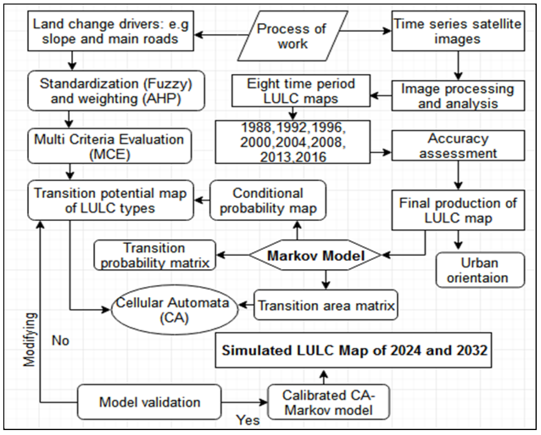
2. Methodology

2.1. Study Area

The study area is located in the central east part of Nepal. Administratively, it incorporates 24 cities of the Kathmandu valley, (Kathmandu: 11 cities, Lalitpur: three cities, and Bhaktapur: four cities) and the Kabhrepalanchok (6 cities) district (CKVAKD) from four districts covering a total area of 1215.23 km². It is geographically enclosed between the northern latitudes of 27°31′40″ and 27°49′10″ and the eastern longitudes of 85°11′18″ and 85°43′44″ (Figure 1). The elevation of the area ranges from 546 to 2825 m above sea level (masl). Population and economic growth are the two major underlying elements that play vital roles in urban land expansion [17,19,33,38,59,60,61,62,63,64] of the region. Economic opportunities in the city’s core areas, population growth in the fringes, and the political situation in the rural areas have mainly contributed to the urbanization of the Kathmandu valley [20,25,65]. Furthermore, rural urban migration, economic centrality, sociopolitical factors, and real estate boom are the drivers of the valley area [55]. According to Central Bureau of Statistics (CBS), 2011, the total population of these four districts was 1,431,699 in 1991, which increased to 2,032,764 in 2001, and 2,900,971 in 2011 [49].

2.2. Data

In this study, freely available maximum cloud-free time-series Landsat images for the years 1988, 1992, 1996, 2000, 2004, 2008, 2013, and 2016 (TM, ETM, and OLI) were obtained from the United State Geological Survey (USGS) website https://earthexplorer.usgs.gov (

Table 1. Dates of the Landsat Time series 5, 7, and 8 images (Landsat 5, hereafter Thematic Mapper (TM); Landsat 7, hereafter Enhanced Thematic Mapper Plus (ETM+); and Landsat 8, hereafter Operational Land Image (OLI).

Year	1988	1992	1996	2000	2004	2008	2013	2016
Months	3 April	23 October	18 October	22 November	15 April	20 November	18 November	12 February
Sensor	TM	TM	TM	ETM	TM	TM	OLI	OLI

) [66]. All the acquired images were post-monsoonal from 23 October to 3 April. In addition, all the images and Shuttle Rader Topographical Mission (SRTM) digital elevation model (DEM) with 30 m resolution were projected in UTM Zone 45N. Furthermore, high spatial resolution images from Google Earth (http://earth.google.com) of multiple dates and topographical maps published by Survey Department, Government of Nepal, 1995 (scale 1:25,000) [67] were collected. The administrative boundary vector data at the district and municipal levels were acquired from the Survey Department of Nepal, and district level population information of 1991, 2001, and 2011 from the Central Bureau of Statistics (CBS) [49]. Major land-cover change information and road networks were gathered using Global Positioning System (GPS) in course of the field visit and field verification campaigns during June 2015 and July 2016.

2.3. Pre-Processing of Images and Design of Image Classification

TM, ETM+, and OLI Landsat images were verified for geometric accuracy and all images were processed in an ENVI environment [33]. These multispectral images were atmospherically and geometrically corrected in course of pre-processing [68,69]. In this study, L1T (terrain corrected) images were converted from digital number (DN) to radiance, and image processing functions were conducted applying the radiometric calibration model. ENVI included radiance calibration, geometric correction, and atmospheric correction. The FLAASH atmospheric correction model was employed using radiance image by applying the appropriate model on the location of the study area. The positional root mean square (RMS) error of geometric rectification was not more than 0.5 pixels. A supervised approach support vector machines (SVM) classifier [18,70] was employed for the classification of LULC and change analysis. Several previous authors have evaluated the performance of SVM algorithms and concluded that it is one of the flexible supervised classifier options with high accuracy [68,70,71,72,73,74]. SVM is a supervised, non-linear, non-parametric classification technique that is widely used in the remote sensing field due to its specific capability to draw conclusions even with limited training samples [75]. Previously, Lee [76] evaluated the SVM algorithms for landslide vulnerability mapping in the Gangwon province of Korea and the results suggested that SVM was quite suitable for a wide range of classification problems, even if the problems were of high dimension and were non-linear separable. Moreover, the approach was applied by Mahmoud et al. [71] to monitor urbanization in Abuja, Nigeria. Schneider [70] evaluated the maximum likelihood classifier (ML), decision tree (DT), and SVM algorithms for monitoring land-cover change in urban and peri-urban areas using Landsat satellite data. This research illustrated that the overall accuracy result, the DT and SVM performed better than the ML classifier. Waske and Benediktsson [77] compared the SVM classification outputs with other algorithms like DT and ML. Based on the results, SVMs achieved the highest overall accuracies of all approaches when classifying the multispectral data. Nevertheless, SVMs formulations are not completely free from drawbacks. The major problem concerns the selection of kernels [76,78]. Despite this limitation, SVMs are still more popular and produce more accurate classification results than the traditional methods [76,78,79]. SVMs can be generally grouped into four kernel functions—namely, linear, polynomial, radial basic function, and sigmoid [78]. The mathematical representations of each kernel are mentioned in the help section of ENVI version 5.3; whereas, the same mathematical representations are presented by Lee et al. [76] using ENVI version 4.4.

In this current study, a communally used radial basis function (RBF) kernel was recognized during image classification [18]. The RBF kernel is frequently used for its advantage in the classification of remotely sensed images to achieve better results than other kernels (polynomial, linear, and sigmoid) [68,80]. The penalty parameter maximum value 100 was assigned and the land-cover classification scheme was adopted as recommended by Anderson et al. [81] and Thapa and Murayama [25]. After the extensive field survey, six main land-use classes were identified: urban/built-up, cultivated land, vegetation cover (dense forest, scattered forest, shrub, and grass), sand area, water body, and open field (

Table 2. Land-cover classification scheme.

LULC Types	Description
Sand Area (SA)	Sand area, river bank, cliffs/small landslide, bare rocks
Water body (WB)	River, lake/pond, canal, reservoir
Open field (OF)	Playground, Park
Vegetation cover (VC)	Evergreen broad leaf forest, deciduous forest, scattered forest, low density sparse forest, degraded forest, Mainly grass field- (dense coverage grass, moderate coverage grass and low coverage grass)
Urban/Built-up (UB)	Commercial areas, urban and rural settlements, industrial areas, government secretariat areas, royal palace construction areas, traffic, airports, public service areas (e.g., school, college, hospital)
Cultivated land (CL)	Wet and dry croplands, orchards

).

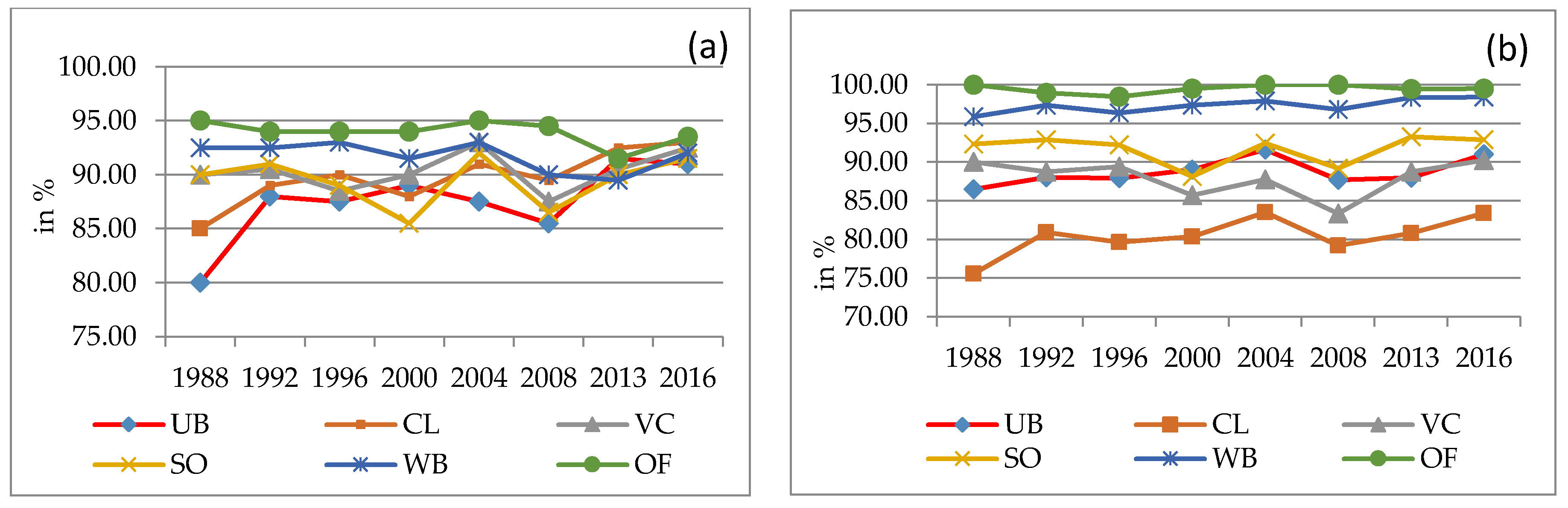
2.4. Accuracy Assessment

In this study, overall accuracy (OA), user’s accuracy (UA), and producer’s accuracies (PA) were observed based on field reference data; topographical maps published by Survey Department, Government of Nepal, 1995 (scale 1:25,000) [67]; and high spatial resolution images of Google Earth (http://earth.google.com) from multiple dates. A total of 1200 (i.e., 200 for each class) stratified random sample points were selected for the validation of classified images for each year.

2.5. Measuring Urban/Built up Area Expansion Rate

To calculate the urban expansion growth rate of the study area, the total transformation of the urban area was taken into consideration [50]. The urban expansion rate refers to the average annual urban area growth in the following years.

$$\mathrm{BER}=(B2-B1)/(T2-T1)$$

(1)

where BER measures the urban expansion rate in (km²/year); B₁, B₂ represents the urban area (km²) in the year; and T₁, T₂ indicates the time.

2.6. Quantification of LULC Based Transition Analysis

The cross function has been applied to create the transition matrix of LULC using TerrSet software developed by Clark Lab (clarklabs.org). The transition matrix consisted of rows and columns of landscape categories at time T₁ and T₂ [50]. In this study, the Land Change Modeler (LCM) system of TerrSet software was applied to create the transition of a LULC map for seven time periods: 1988 and 1992; 1992 and 1996; 1996 and 2000; 2000 and 2004; 2004 and 2008; 2008 and 2013; and 2013 and 2016.

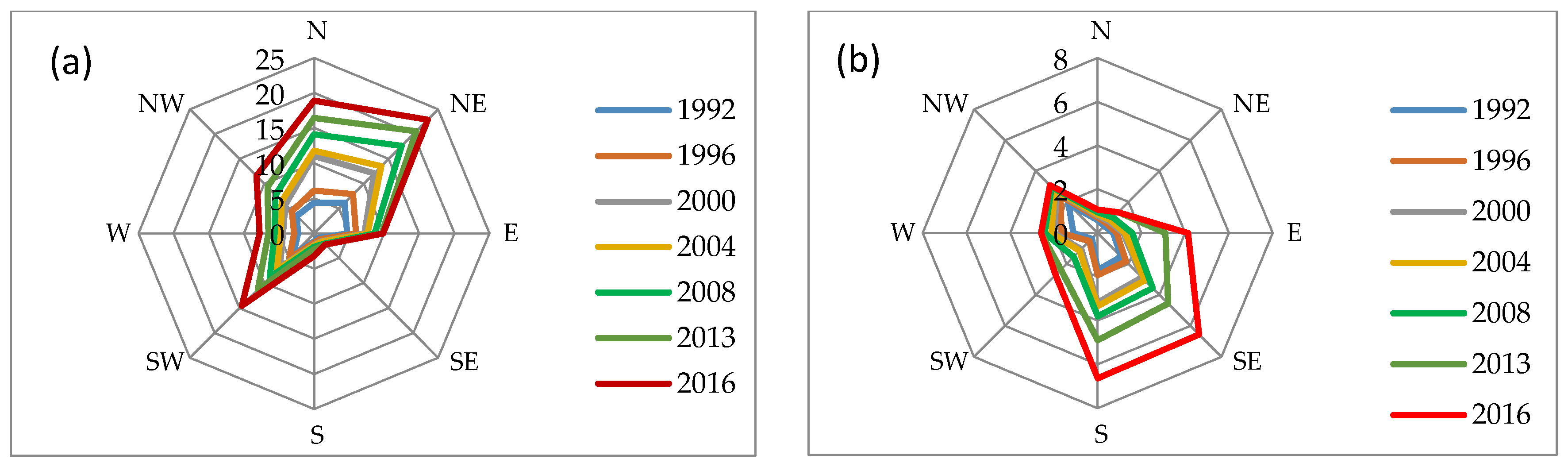
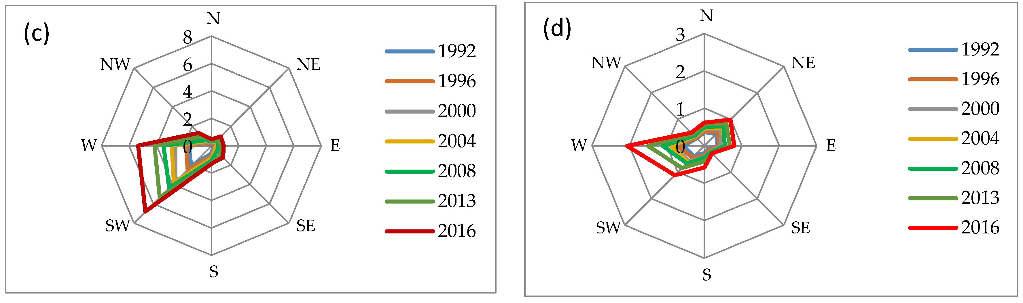
2.7. Urban Expansion and Orientation

Despite its wide range of significance, few studies [82,83] have quantified the landscape structure using landscape metrics and explored the orientation of urban expansion [50,84,85]. Cushman et al. [83] applied the FRAGSTATS software and principal component analysis (PCA) for the evaluation of landscape structure, and cluster analysis was conducted. The same software package FRAGSTATS was employed to detect the gradient of landscape pattern along two directions: W-E and SW-NE [82]. To analyze the spatial changes of urban expansion, Singadurbar of Kathmandu, Lagankhel of Lalitpur, Kamalbinayak of Bhaktapur, and Dhulikhel of Kavrepalanchok districts were assumed (Figure 1) as centers. Identification of the assumed city centers of each district were based on the field visit experience of the authors and classified satellite images from 1988. The outcomes should answer the questions of where and in which direction the changes mostly occurred from the city core [50]. District level urban orientation was observed through the linings created by utilizing ArcGIS 10.1. The waves [84] consisted of eight subdivisions: North, North-East, East, South-East, South, South-West, West, North-West, North (N-NE, NE-E, E-SE, SE-S, S-SW, SW-W, W-NW, and WN-N), each representing 45° from the central point (Figure 1).

2.8. Simulation of LULC Change

CA–Markov is an appropriate technique for modeling LULC change in places where understanding and describing landscape relations are difficult. This model allows the future status of an ecosystem based on its pre-existing status to be predicted. The CA–Markov model has been widely used to effectively understand and measure urban expansion [33] and landscape dynamics [86]. Typically, the implementation process of the CA–Markov model consists of: (1) the preparation of LULC maps with the same time interval (here, 2000, 2008, and 2016); (2) the calculation of transition area matrices based on LULC maps; (3) the generation of transition potential maps using driving factors; (4) evaluating the model’s ability to simulate future changes based on kappa indices; and (5) simulating the LULC maps for the coming years (here, 2024 and 2032).

The transition matrix file was calculated using the Markov model in TerrSet software. A transition area matrix records the number of cells that are expected to change from one land-cover class to another in a given period in the future. In this part, transitional area matrices were generated based on the historical LULC information from 2000–2008, 2008–2016, and 2000–2016 to explore how each land-cover was projected to change. Detailed study framework has been presented in Figure 2.

To produce transition potential maps, multi-criteria evaluation (MCE), analytic hierarchy process (AHP), and fuzzy membership function were applied. The AHP method was applied to determine the weights of driving factors with the use of pairwise evaluations [87]. The AHP method allows weighting of land-cover transition potential on the basis of a set of potential maps (e.g., magnitude of slope), and incorporates growth constraints. This GIS-based AHP is a strong tool because of its high ability to incorporate different types of heterogeneous variables and its simplicity to gain the weights of suitable variables [88,89]. The transition potential maps indicate the ability of a pixel to turn from one state to another or remain unchanged. According to the conditions of each region, different driving factors are used to produce transition potential maps. Here, based on previous studies [18,43,81], the following driving factors were chosen: (a) distance to water bodies; (b) distance to main roads; (c) distance to built-up areas; and (d) slope. Fuzzy membership functions (e.g., linear monotonic increase function) were used to standardize the driver maps into a 0–1 range, where 0 represents unsuitable locations and 1 represents ideal locations. The AHP technique was then run for weighting and specifying priorities regarding the relative importance of the driving factors. The details of the weights and control points are listed in

Table 3. Extracted weights based on analytic hierarchy process (AHP) and fuzzy standardization for urban areas.

Control Points	Functions	Weights	Factors
0–500 m highest suitability	J-shaped	0.28	Distance from main roads
500–5000 m decreasing suitability
>5000 m no suitability
0–100 m no suitability	Linear	0.15	Distance from water bodies
100–7500 m increasing suitability
>7500 m highest suitability
0–100 m highest suitability	Linear	0.38	Distance from built-up areas
100–5000 km decreasing suitability
>5000 km no suitability
0% highest suitability	Sigmoid	0.19	Slope
0–15% decreasing suitability
>15% no suitability

.

Then, Kappa variations were employed to evaluate the model by comparing the LULC map of 2016 with the simulated map of 2016. The standard accuracy of the models, which was not less than 80%, determined that they were potent predictive tools [32,37]. In the present study, Kno, Kstandard, and Klocation were used to validate the model. Descriptions of these Kappa indices are summarized in Keshtkar and Voigt [32]. Finally, the LULC map of 2016 was set as the base map, and the transition area matrices of 2000–2008 and 2008-2016 were used to forecast the LULC maps of 2024 and 2032, respectively.

3. Result and Discussion

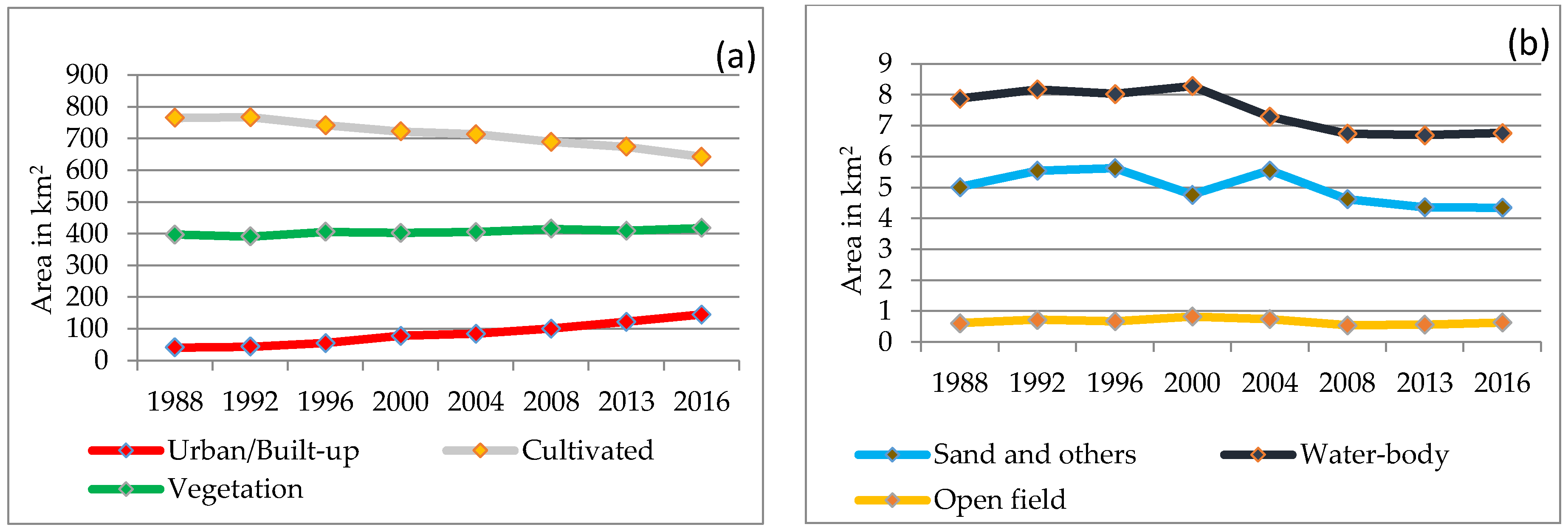
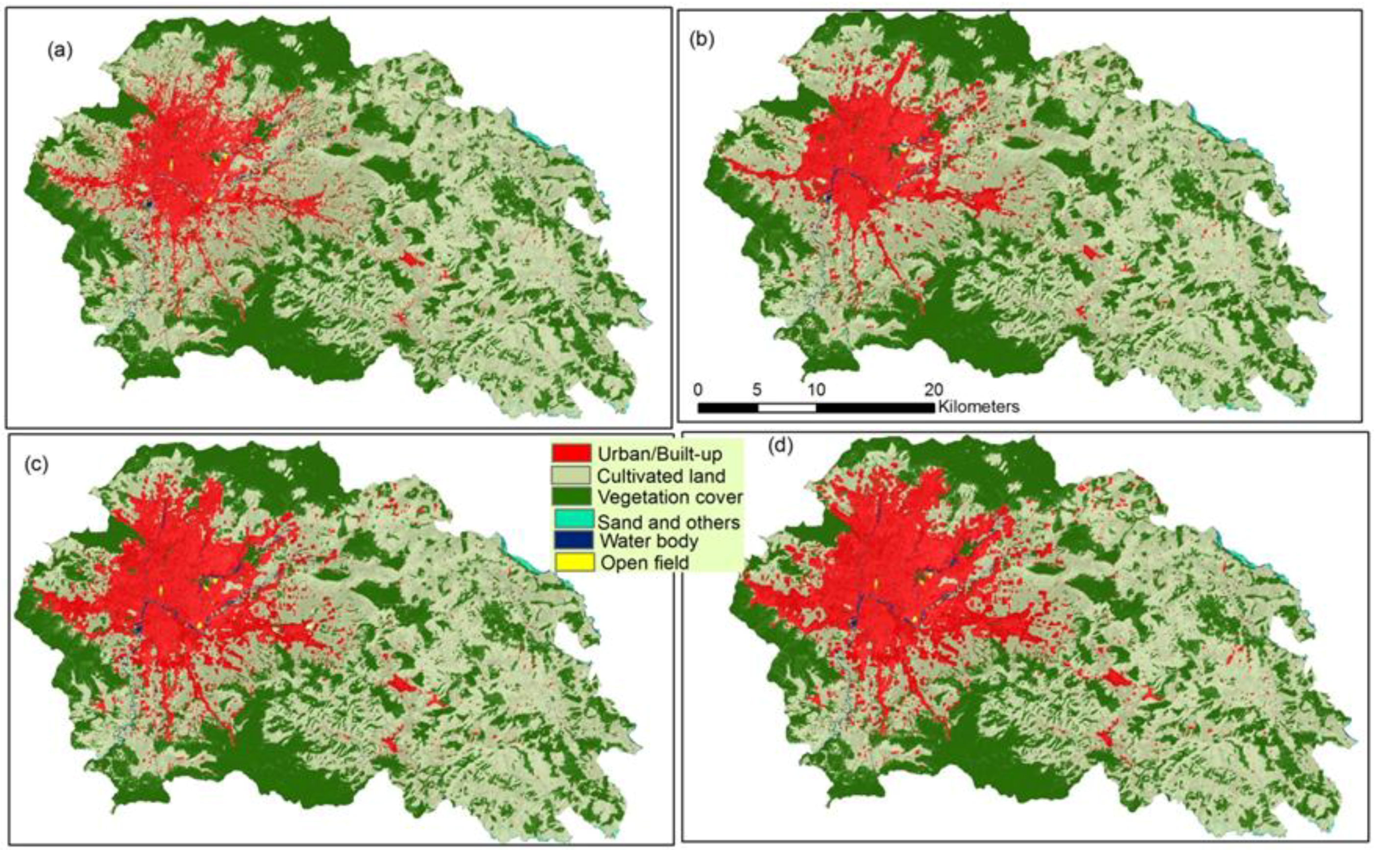
3.1. LULC Change

In this study, the overall classification accuracy (OA) of the LULC maps for 1988 (88.75%), 1992 (90.83%), 1996 (90.33%), 2000 (89.67%), 2004 (91.92%), 2008 (88.92%), 2013 (90.92%), and 2016 (92.25%) were derived. The user’s accuracy (UA) and producer’s accuracy (PA) for the LULC maps of each year are presented in Figure 3a,b, respectively.

Figure 4 shows the spatiotemporal distribution of LULC dynamics from 1988 to 2016. The extent of the land-cover types varied across the years. LULC analysis explored the significant transformations in several land-use classes between 1988 and 2016 (Figure 3,

Table 4. LULC statistics from 1988 to 2016.

LULC	1988		1992		1996		2000		2004		2008		2013		2016
	km2	%	km2	%	km2	%	km2	%	km2	%	km2	%	km2	%	km2	%
UB	40.53	3.33	43.45	3.58	54.59	4.49	77.71	6.39	84.3	6.94	100.35	8.26	121.59	10.01	144.35	11.88
CL	764.87	62.94	766.72	63.09	741.31	61	721.85	59.4	712.78	58.65	688.57	56.66	673.61	55.43	641.96	52.83
VC	396.33	32.61	390.63	32.14	405.01	33.33	401.81	33.06	404.56	33.29	414.41	34.1	408.42	33.61	417.17	34.33
SA	5.02	0.41	5.54	0.46	5.62	0.46	4.75	0.39	5.55	0.46	4.62	0.38	4.36	0.36	4.35	0.36
WB	7.87	0.65	8.17	0.67	8.02	0.66	8.28	0.68	7.29	0.6	6.74	0.55	6.69	0.55	6.76	0.56
OF	0.61	0.1	0.72	0.1	0.67	0.1	0.82	0.1	0.74	0.1	0.1	0.104	0.56	0.1	0.63	0.1
Total	1215	100	1215	100	1215	100	1215	100	1215	100	1215	100	1215	100	1215	100

).

Major changes observed were the significant increase of urban/built-up areas and a sharp decline of cultivated land area. The built-up area increased by 103.82 km² from 40.53 km² (3.33%) in 1988 to 144.35 km² (11.88%) in 2016 with an average annual growth rate of 9.15%. In contrast, cultivated land decreased by 122.91 km² from 764.87 km² (62.94%) in 1988 to 641.96 km² (52.83%) in 2016 (

Table 5. LULC magnitude from 1988 to 2016 (in km²).

LULC	1988–1992	1992–1996	1996–2000	2000–2004	2004–2008	2008–2013	2013–2016	1988–2016
U/B	2.93	11.14	23.11	6.60	16.04	21.24	22.77	103.83
CL	1.85	−25.41	−19.46	−9.07	−24.21	−14.96	−31.65	−122.91
VC	−5.70	14.38	−3.20	2.75	9.85	−5.98	8.75	20.84
SA	0.52	0.09	−0.87	0.80	−0.93	−0.26	−0.01	−0.67
WB	0.30	−0.14	0.26	−0.99	−0.55	−0.06	0.07	−1.11
OF	0.11	−0.05	0.15	−0.08	−0.20	0.02	0.07	0.02

).

Vegetation coverage increased by 20.85 km², from 396.32 km² (32.61%) to 417.17 km² (34.33%) (Table 4, Figure 5a,b). The majority of the urban area was sourced from cultivated land. Specifically, 93.49%, 98.56%, 95.45%, 91.66%, 97.81%, 97.12%, and 98.63% were gained from cultivated land alone during 1988-1992, 1992–1996, 1996–2000, 2000–2004, 2004–2008, 2008–2013, and 2013–2016, respectively.

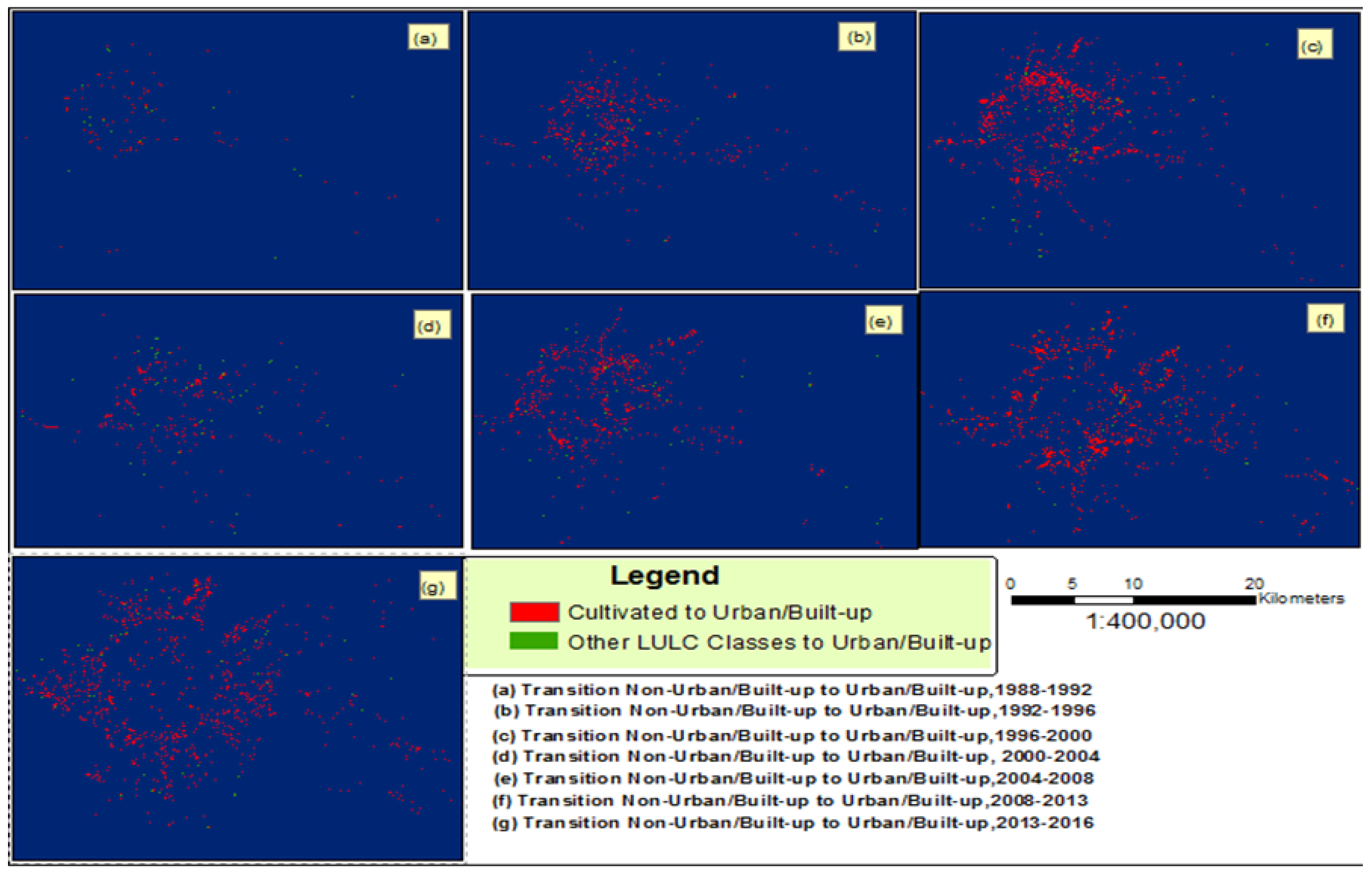
3.2. Spatiotemporal Transition of LULC

Despite the overall expansion in urban/built-up areas, the expansion pattern varied across individual time periods as briefly outlined below:

Period one (1988–1992): The speed of urban expansion was slower before 1992 and accelerated remarkably in the preceding periods due to socioeconomic and political factors. Increase in urban/built-up areas and cultivated land and the decline in vegetation were the major transformations observed. Urban area increased by 2.92 km² from 40.53 km² to 43.45 km² with an annual average growth rate of 1.8%. This was due to the transformation of remaining land-use classes, mainly 2.73 km² of cultivated land area into urban/built-up areas (Figure 6a). Vegetation cover declined by 5.69 km², from 396.32 km² to 390.63 km² due to the conversion of 11.97 km² of vegetation cover into cultivated land. With this, cultivated land increased by 1.85 km², from 764.87 km² to 766.72 km².

Period two (1992–1996): Increase in urban/built-up areas and vegetation cover and decrease of cultivated land were the three important changes witnessed during this period. Urban area increased by 11.14 km² from 43.45 km² to 54.59 km² with an average annual growth rate of 6.41%. Urban parks, forest reserves, and forest resorts maintained the vegetation cover within the Kathmandu valley [55]. The expansion of urban/built-up areas and the sharp decline of cultivated land was mainly because 10.98 km² of cultivated land was converted into urban/built-up areas (Figure 6b). The increase in forest area was closely associated with the community-based forest management biodiversity practice from 1975, the program launched across in Nepal after 1995 intended to conserve and rehabilitate degraded forest resources [90], which has been successful in achieving a significant increase in forest cover and density not only in the study area, but in the hill region of Nepal [91].

Period three (1996–2000): Gradual increase in urban/built-up and continuous decline of cultivated land are the two major transformations observed during this period (Figure 6c). Urban areas increased by 23.11 km², from 54.59 km² to 77.7 km² with an average annual growth rate of 10.58%. The country confronted a decade-long political upheaval from 1996 to 2006, which enforced internal mass migration to the cities [47]. Urban in-migration contributed around 40% of the population growth of the Kathmandu valley in the 1990s. Due to high migration and population growth, the real estate market culminated after 1999 and vigorously continued in the preceding years [55]. This led to intense pressure upon the cultivated land resulting in a decrease of 23.23 km² from 741.31 km² to 718.08 km² over the period.

Period four (2000–2004): The trend of urban increase and decline of cultivated land also continued during this period. Urban areas increased by 6.6 km², from 77.7 km² to 84.3 km² with an average annual growth rate of 2.12%. Of the expanded urban area, 6.05 km² was sourced from cultivated land. Since the political turmoil peaked during this period, the trend of in-migration continued. More than 500,000 refugees were displaced and accommodated inside the valley [92], resulting in the land price increasing by more than 300% since 2003 [55]. The flourishing land market influenced aggressive urban area expansion, and cultivated land declined by 5.3 km², from 718.08 km² to 712.78 km² (Figure 6d).

Period five (2004–2008): Remarkable increase in the urban/built-up areas and vegetation cover, as well as a sharp decline of cultivated land were witnessed during this period. Urban area increased by 16.05 km², from 84.30 km² to 100.35 km² with an annual average growth rate of 4.75%. The continuous shift of people towards the Kathmandu valley as well as city centers from rural areas was also driven by access to public services and economic opportunities [20,25,65]. Despite the alteration of 9.8 km² vegetation cover into cultivated land, it dropped by 24.21 km², from 712.78 km² to 688.57 km². This increase was mainly driven by the conversion of 15.7 km² of cultivated land into urban areas and 20.36 km² into vegetation cover. The Shivpuri Nagarjun wild life reserve area was upgraded to a national park status in 2002. Additionally, strongly managed community forests have played key roles in the protection of the vegetation cover [55] (Figure 6e).

Period six (2008–2013): Continuous expansion of urban/built-up areas and a decline of cultivated land and vegetation cover were investigated during this period (Figure 6f). The urban area increased by 21.24 km², from 100.35 km² to 121.59 km², with an average annual growth rate of 4.23%. Cultivated land declined by 14.96 km², from 688.57 km² to 673.61 km² because 20.63 km² of cultivated land changed into urban areas and 6.47 km² into vegetation cover. The Kathmandu valley is a gateway and central touristic hub with several heritages which receives 90% of the tourists in the country. Hence, the infrastructure to cope with the huge influx of tourists was developed at the expense of cultivated land in the valley [92].

Period seven (2013–2016): Increases in urban/built-up areas and vegetation cover, and a decrease in cultivated land were the major changes observed during this period. Urban areas increased by 22.76 km², from 121.59 km² to 144.35 km² with an average annual growth rate of 6.23%. In contrast, cultivated land declined by 31.65 km², from 673.61 km² to 641.96 km². Vegetation cover increased by 8.75 km², from 408.42 km² to 417.17 km². All these changes were associated with the conversion of 22.45 km² of cultivated land into urban areas and 14.86 km² into vegetation cover (Figure 6g).

3.3. Urban Area Expansion and Orientation

Exploring where urbanization has occurred is important when determining how urbanization may be better managed in the future, and the city center is usually active in socioeconomic activities [61]. In our analysis, the “center” generally referred to the urban center [33,85] and the assumed urban area gradually decreased outwards. Although, the essentiality to explore the orientation and extent of urban expansion exists, few studies have attempted it [50,84]. For the orientation and extent analysis, we assumed Dhulikhel in Kabhrepalanchok, Kamalbinayak in Bhaktapur, Lagankhel in Lalitpur, and Singhadurbar in Kathmandu as the urban centers since they were the socioeconomic hubs where urbanization took place since the initial phase of our study, which was 1988.

According to the study, every direction from the city core has gained a remarkable urban increase, however, expansion and density has gradually decreased outside the assumed centers. The urban area of Kathmandu was limited to 25.43 km² in 1988, which gradually increased to 27.25 km² in 1992, 34.77 km² in 1996, and aggressively increased to 50.6 km² in 2000. The expansion trend continued and reached 55.06 km² in 2004, 66.53 km² in 2008, 78.44 km² in 2013, and 90.97 km² in 2016. The N-NE (Tokha, Budhanilkantha areas), NE-E (Shankarapur and Kageshwori Manohara areas), SW-W (Chandragiri and Kirtipur areas), NW-N (Tarakeshwor area), and E-SE (Baneshwar and Airport area) directions were highly urbanized while the W-NW (Nagarjun area) direction was relatively less urbanized. Regarding the SE-S direction, almost the entire area was urban, and the boundary was adjoined with the densely settled Lagankhel of Lalitpur district. The S-SW (Dakshinkali area) direction was comparatively less urbanized (Figure 7a).

Peripheral areas of the assumed city center, Lagankhel in Lalitpur district have been densely settled for several years. The total urban coverage of the district during 1988 was 7.73 km², which increased to 8.33 km² in 1992 to 28.12 km² in 2016. The SW-W, W-NW, NW-N, N-NE, and NE-E directions were highly urbanized, but were relatively transected as smaller urban clusters during the course of the study. East sprawl was relatively complacent (Figure 7b). The areas at the proximity to the road networks were more urbanized. Higher urban enlargement was reported in the Lubhu, Lamatar, and Chapagaun areas of Lalitpur [50].

Bhaktapur is one of the most important gateways to the Kathmandu valley and consists of a large plain area where urban sprawl is more prevalent. The total urban coverage accounted for 4.8 km² in 1988 that gradually increased to 5.1 km² in 1992, and to 18.27 km² in 2016. The majority of the urban area expanded towards the SW-W (Balkot, Katunje, Sirutar, and Dadhikot areas) and W-NW (Madhyapur Thimi, Duwakot) directions; whereas the N-NE (Chhaling area) and E-SE (Tathali and Chipatol area) directions gained comparatively lower urban expansion (Figure 7c).

Peripheral areas of the assumed center, Dhulikhel in Kabhrepalanchok district have also been densely settled for several years. The total urban coverage of district during 1988 was 2.55 km², which increased to 6.93 km² in 2016. The highest urban expansion occurred in the SW-W and W-NW (Panauti, Dhulikhel, and Banepa areas) directions. Similarly, medium expansion was witnessed towards the E-SE, NE-E, and N-NE (Panchkhal, Mandandeupur, and Namobudda areas), and relatively lower expansion has taken place towards the SE-S, S-SW, and NW-N directions (Dapcha and Balthali areas) (Figure 7d).

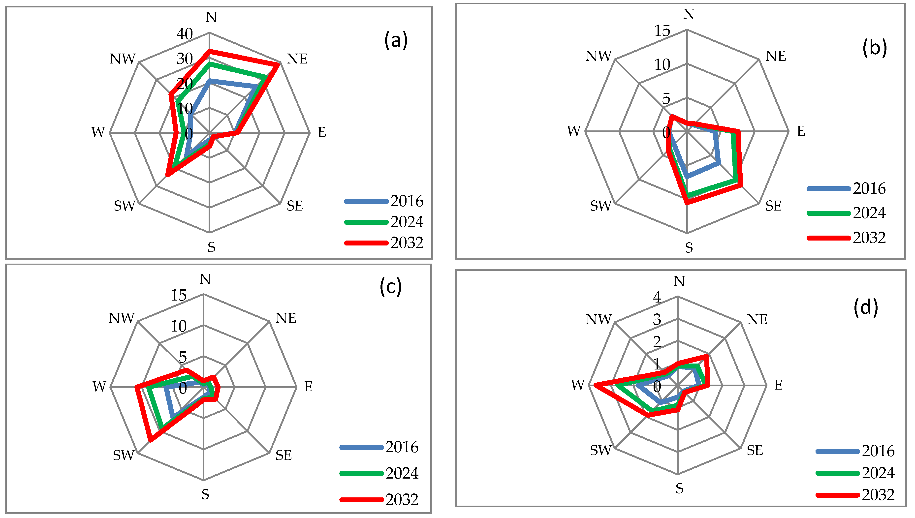
3.4. CA–Markov Model

In this study, the transition probability matrices produced by the Markov model prepared the details on the probability of transition between LULC types during the periods 2000–2008 and 2008–2016 (

Table 6. Transition probability matrix of LULC classes for the periods 2000–2008, 2008–2016, and 2000–2016.

	LULC	UB	CL	VC	SA	WB	OF
2000–2008	UB	0.8949	0.0447	0.0250	0.0203	0.0152	0.0000
	CL	0.0742	0.8445	0.0771	0.0030	0.0006	0.0005
	VC	0.0117	0.1371	0.8774	0.0022	0.0016	0.0001
	SA	0.0768	0.2050	0.0282	0.5903	0.1195	0.0002
	WB	0.0725	0.0644	0.0493	0.0728	0.7409	0.0000
	OF	0.0961	0.2916	0.0926	0.0036	0.0036	0.7226
2008–2016	UB	0.9121	0.0618	0.0205	0.0088	0.0150	0.0018
	CL	0.1087	0.8237	0.0435	0.0021	0.0014	0.0007
	VC	0.0181	0.0850	0.8738	0.0013	0.0013	0.0005
	SA	0.0703	0.2191	0.0378	0.5902	0.0823	0.0002
	WB	0.0474	0.0622	0.0251	0.0808	0.6945	0.0000
	OF	0.1169	0.1674	0.0178	0.0040	0.0059	0.6880
2000–2016	UB	0.8935	0.0380	0.0278	0.0192	0.0192	0.0024
	CL	0.1080	0.8165	0.0622	0.0022	0.0008	0.0004
	VC	0.0296	0.0931	0.8738	0.0017	0.0016	0.0001
	SA	0.0915	0.2404	0.0251	0.6234	0.1096	0.0000
	WB	0.1004	0.1680	0.0360	0.0668	0.7399	0.0000
	OF	0.1125	0.1513	0.0437	0.0049	0.0170	0.7007

Note: UB (Urban /Built-up), CL (Cultivated Land), VC (Vegetation Cover), SC (Sand Area), WB (Water Body), OF (Open Field).

).

Models with accuracies in excess of 80% are typically considered very strong predictive tools [32,37]. In evaluating the overall accuracy, using the value of Kno is better than the Kstandard [93]. The Kno value was 0.91, which verifies the accuracy of this model. The model performed very well in its overall ability to predict LULC map of 2016 (Kstandard = 0.87), and the Klocation value of 0.88 indicates that the model provides a reasonable representation of location. Thus, based on the results, the CA–MC model is a reliable and powerful tool for predicting LULC changes.

These results showed that the probability of future changes of vegetation to cultivated land from 2000 to 2008 was 13.71%. This likelihood of transition decreased reasonably to 8.5% in 2016. Of all the phenomena, built-up areas experienced the largest increase between the first and second projections. After eight years (during 2024), there was an 89.5% chance a current built-up pixel would remain part of the status quo, however, after sixteen years (during 2032), this value would increase to 91.1%. Cultivated areas possessed the highest likelihood of changing into built-up areas for both periods.

According to the analysis, 11.88% of the entire study area was occupied by urban land in 2016 (

Table 7. Distribution of LULC categories (in km²) and percentage of changes for 2016–2032.

	Year			Change in LULC Structure
	2016	2024	2032	Δ%2016–2024	Δ%2024–2032	Δ%2016–2032
UB	144.35	200.16	238.17	27.88	15.96	39.39
CL	641.96	587.28	555.48	−9.31	−5.73	−15.57
VC	417.12	413.62	405.97	−0.85	−1.88	−2.75
SA	4.35	5.52	6.87	21.2	19.65	36.68
WB	6.76	8.04	8.13	15.92	1.11	16.85
OF	0.63	0.61	0.60	−3.28	−1.67	−5.0

), which will increase to 19.6% by 2032. The results also showed that the rapid development of urban land would be accompanied by a sharp decline in agricultural and vegetation lands(Table 7) at the expense of other land use types, but mostly at the cost of cultivated land (loss of 15.6%). However, minor loss has been predicted for vegetation cover, from 417.12 km² (34.3%) to 405.97 km² (33.4%) over the respective years (Figure 8).

The results showed that the rapid development of urban land would be accompanied by a sharp decline in agricultural and vegetation land (Table 7). Consequently, in addition to the gradual decline of cultivated land area, this is closely associated with endangering food security and health, and the integrity of the ecosystem will be heavily affected [94]. Urban development is also associated with an increase in population and personal and public transportation [33,94]. Therefore, we can expect an increase in environmental pollutants in the future; and due to the destruction and degradation of natural purifiers (plants and soil), environmental hazards may appear as strong threats to the residents of this region.

Gradual urban expansion in the four individual districts of the study area was predicted from the simulation analysis. Newer settlements will emerge, and existing settlements will be in-filled. The urban area of Kathmandu occupied 90.97 km² in 2016, which is expected to expand to 124.56 km² by 2024 and 148.47 km² by 2032. Furthermore, the urban area is expected to increase significantly in the N-NE, SW-W, W-NW, and NW-N directions (Figure 9a). The outskirt boundaries of Tarakeshwor, Nagarjun, Chandragiri/Kirtipur areas, and the eastern boundary of Shankarapur and Kageshwori Manohara areas are adjoined to hills where less urban expansion can be assumed in the future. Meanwhile, the urban area of Lalitpur district covered 28.12 km² during 2016, which is expected to grow continuously and reach 38.67 km² by 2024 and 41.84 km² by 2032. Higher urban expansion is predicted to occur in the E-SE, SE-S, and S-SW directions (Figure 9b). The trend of urbanization is expected to be outflanked in the city outskirts and hinterland adjacent to road networks. The urban coverage of Bhaktapur totaled 18.27 km², which is predicted to reach 27.77 km² and 37.18 km² by 2024 and 2032, respectively. The majority of urban expansion will take place in the SW-W and W-NW directions (Figure 9c). During 2016, the urban coverage of Kabhrepalanchok district totaled 6.93 km², which is expected to occupy 9.75 km² and 12.08 km² by 2024 and 2032, respectively. The N-NE, NE-E, S-SW, and SW-W directions will experience relatively higher expansion (Figure 9d).

4. Conclusions

The study investigated the spatial–temporal pattern of LULC change, in particular, the urban expansion dynamics of CKVAKD using maximum cloud-free time-series Landsat images between 1988 and 2016. As SVM tends to result in relatively higher accuracy than the ML classifier [70,77], the current study has utilized the SVM algorithm and is able to achieve an overall accuracy of LULC maps between 85% and 93%. The LULC analysis explored the remarkable increase in urban/built-up areas and forest cover and a significant decline of the cultivated land area. Increase in the urban area was assumed to be closely associated with the rise in infrastructure to accommodate the rising population, which in turn has caused losses of prime farm land. Urban expansion has sparked towards the western part of the study area when compared to the eastern section. Urban sprawl was multifaceted and largely attributed to the proximity and accessibility of road networks. Simulation analysis conducted for the years of 2024 and 2032 using a CA–Markov model predicted that urban area will gradually increase in future years while cultivated and vegetation land will continuously remain under pressure. Unmanaged settlement patterns and the continuous urban development process, leading to land fragmentation and pressure in land resources, continue the urban development process [20]. Such unplanned urban sprawl and its detrimental consequences are likely to result in overall environmental disequilibrium in the valley [53,55].

The study assumed the eastern part of the study area as the potential zone for future urban expansion where the opportunities to develop planned and managed urban settlements still exist. Discouraging the haphazard use of urban land, controlling the encroachment of public land, and preparation of better guidelines in terms of physical infrastructure development is highly essential to secure a sustainable urban future [56]. In addition, the government authorities need to enforce strict urban growth policies in coming days [20]. The urbanization process of the study area was driven by population growth, migration, socioeconomic, and political factors. The continuous urban expansion trend in the preceding decades is likely to result in severe environmental disequilibrium. Thus, careful urban planning is always emphasized.

References

1. Guan, D.; Li, H.; Inohae, T.; Su, W.; Nagaie, T.; Hokao, K. Modeling urban land use change by the integration of cellular automaton and markov model. Ecol. Model. 2011, 222, 3761–3772. [Google Scholar] [CrossRef]
2. Sherbinin, A.D. A Ciesin Thematic Guide to Land Land: Use and Land Use and Land Use and Land—Cover Change (LUCC) cover Change (LUCC); Center for International Earth Science Information Network (CIESIN), Columbia University: Palisades, NY, USA, 2002. [Google Scholar]
3. Eastman, J.R.; van Fossen, M.; Solo’rzano, L.A. Transition Potential Modeling for Land-Cover Change, 1st ed.; ESRI Press: Redlands, CA, USA, 2005. [Google Scholar]
4. Rai, R.; Zhang, Y.; Paudel, B.; Li, S.; Khanal, N. A synthesis of studies on land use and land cover dynamics during 1930–2015 in bangladesh. Sustainability 2017, 9, 1866. [Google Scholar] [CrossRef]
5. Briassoulis, H. Analysis of Land Use Change: Theoretical and Modeling Approaches; Regional Research Institute, West Virginia University: Morgantown, WV, USA, 2000. [Google Scholar]
6. Bal Kumar, K.C. Internal Migration in Nepal, Population Monograph of Nepal; Central Bureau of Statistics: Kathmandu, Nepal, 2003.
7. Seto, K.C.; Fragkias, M.G.B.; Reilly, M.K. A meta-analysis of global urban land expansion. PLoS ONE 2011, 6. [Google Scholar] [CrossRef] [PubMed]
8. Yuan, F.; Sawaya, K.E.; Loeffelholz, B.C.; Bauer, M.E. Land cover classification and change analysis of the twin cities (minnesota) metropolitan area by multitemporal landsat remote sensing. Remote Sens. Environ. 2005, 98, 317–328. [Google Scholar] [CrossRef]
9. Sun, C.; Wu, Z.-F.; Lv, Z.-Q.; Yao, N.; Wei, J.-B. Quantifying different types of urban growth and the change dynamic in guangzhou using multi-temporal remote sensing data. Int. J. Appl. Earth Obs. Geoinform. 2013, 21, 409–417. [Google Scholar] [CrossRef]
10. Zhao, M.; Cheng, W.; Zhou, C.; Li, M.; Huang, K.; Wang, N. Assessing spatiotemporal characteristics of urbanization dynamics in southeast asia using time series of dmsp/ols nighttime light data. Remote Sens. 2018, 10, 47. [Google Scholar] [CrossRef]
11. Lu, Q.; Chang, N.-B.; Joyce, J.; Chen, A.S.; Savic, D.A.; Djordjevic, S.; Fu, G. Exploring the potential climate change impact on urban growth in london by a cellular automata-based markov chain model. Comput. Environ. Urban Syst. 2017, 68, 121–132. [Google Scholar] [CrossRef]
12. Li, X.; Yeh, A.G.-O. Modelling sustainable urban development by the integration of constrained cellular automata and GIS. Int. J. Geogr. Inform. Tion Sci. 2000, 14, 131–152. [Google Scholar] [CrossRef]
13. Wu, K.-Y.; Zhang, H. Land use dynamics, built-up land expansion patterns, and driving forces analysis of the fast-growing hangzhou metropolitan area, eastern China (1978–2008). Appl. Geogr. 2012, 34, 137–145. [Google Scholar] [CrossRef]
14. Dubovyk, O.; Sliuzas, R.; Flacke, J. Spatio-temporal modelling of informal settlement development in sancaktepe district, istanbul, turkey. ISPRS J. Photogramm. Remote Sens. 2011, 66, 235–246. [Google Scholar] [CrossRef]
15. Poelmans, L.; Van Rompaey, A. Detecting and modelling spatial patterns of urban sprawl in highly fragmented areas: A case study in the flanders–brussels region. Landsc. Urban Plan. 2009, 93, 10–19. [Google Scholar] [CrossRef]
16. Cohen, B. Urbanization in developing countries: Current trends, future projections, and key challenges for sustainability. Technol. Soc. 2006, 28, 63–80. [Google Scholar] [CrossRef]
17. Shafizadeh Moghadam, H.; Helbich, M. Spatiotemporal urbanization processes in the megacity of Mumbai, India: A markov chains-cellular automata urban growth model. Appl. Geogr. 2013, 40, 140–149. [Google Scholar] [CrossRef]
18. Rimal, B.; Zhang, L.; Keshtkar, H.; Sun, X.; Rijal, S. Quantifying the spatiotemporal pattern of urban expansion and hazard and risk area identification in the kaski district of nepal. Land 2018, 7, 37. [Google Scholar] [CrossRef]
19. Dewan, A.M.; Yamaguchi, Y. Using remote sensing and GIS to detect and monitor land use and land cover change in dhaka metropolitan of bangladesh during 1960–2005. Environ. Monit. Assess. 2009, 150, 237–249. [Google Scholar] [CrossRef] [PubMed]
20. Thapa, R.B.; Murayama, Y. Scenario based urban growth allocation in Kathmandu valley, nepal. Landsc. Urban Plan. 2012, 105, 140–148. [Google Scholar] [CrossRef]
21. Jiang, B.; Yao, X. Geospatial analysis and modeling of urban structure and dynamics: An overview. In Geospatial Analysis and Modelling of Urban Structure and Dynamics; Jiang, B., Yao, X., Eds.; Springer: Dordrecht, The Netherlands, 2010; pp. 3–11. [Google Scholar]
22. Jokar Arsanjani, J.; Helbich, M.; Kainz, W.; Darvishi Boloorani, A. Integration of logistic regression, markov chain and cellular automata models to simulate urban expansion. Int. J. Appl. Earth Obs. Geoinform. 2013, 21, 265–275. [Google Scholar] [CrossRef]
23. Hopkins, L.D.; Kaza, N.; Pallathucheril, V.G. A Data Model to Represent Plans and Regulations in Urban Simulation Model, 1st ed.; ESRI: Redlands, CA, USA, 2005. [Google Scholar]
24. Campbell, J.B. Introduction to Remote Sensing; The Guilford Press: New York, NY, USA, 1996. [Google Scholar]
25. Thapa, R.B.; Murayama, Y. Examining spatiotemporal urbanization patterns in Kathmandu valley, nepal: Remote sensing and spatial metrics approaches. Remote Sens. 2009, 1, 534–556. [Google Scholar] [CrossRef]
26. Cheng, J.; Masser, I. Urban growth pattern modeling: A case study of wuhan city, pr China. Landsc. Urban Plan. 2003, 62, 199–217. [Google Scholar] [CrossRef]
27. Mas, J.-F.; Kolb, M.; Paegelow, M.; Camacho Olmedo, M.T.; Houet, T. Inductive pattern-based land use/cover change models: A comparison of four software packages. Environ. Model. Softw. 2014, 51, 94–111. [Google Scholar] [CrossRef] [Green Version]
28. Wu, D.; Liu, J.; Wang, S.; Wang, R. Simulating urban expansion by coupling a stochastic cellular automata model and socioeconomic indicators. Stoch. Environ. Res. Risk Assess. 2010, 24, 235–245. [Google Scholar] [CrossRef]
29. Allen, J.; Lu, K. Modeling and prediction of future urban growth in the charleston region of south carolina: A gis-based integrated approach. Ecol. Soc. 2003, 8. [Google Scholar] [CrossRef]
30. Cheng, J. Modelling Spatial and Temporal Urban Growth; Utrecht University: Utrecht, The Netherlands, 2003. [Google Scholar]
31. Batty, M.; Xie, Y. Urban Growth Using Cellular Automata Models, 1st ed.; ESRI Press: Redlands, CA, USA, 2005. [Google Scholar]
32. Keshtkar, H.; Voigt, W. A spatiotemporal analysis of landscape change using an integrated markov chain and cellular automata models. Model. Earth Syst. Environ. 2015, 2. [Google Scholar] [CrossRef]
33. Rimal, B.; Zhang, L.; Keshtkar, H.; Wang, N.; Lin, Y. Monitoring and modeling of spatiotemporal urban expansion and land-use/land-cover change using integrated markov chain cellular automata model. ISPRS Int. J. Geo-Inf. 2017, 6, 1–21. [Google Scholar] [CrossRef]
34. Kityuttachai, K.; Tripathi, N.; Tipdecho, T.; Shrestha, R. Ca-markov analysis of constrained coastal urban growth modeling: Hua hin seaside city, thailand. Sustainability 2013, 5, 1480. [Google Scholar] [CrossRef]
35. García, A.M.; Santé, I.; Boullón, M.; Crecente, R. Calibration of an urban cellular automaton model by using statistical techniques and a genetic algorithm. Application to a small urban settlement of nw spain. Int. J. Geogr. Inf. Sci. 2013, 27, 1593–1611. [Google Scholar] [CrossRef]
36. Ke, X.; Qi, L.; Zeng, C. A partitioned and asynchronous cellular automata model for urban growth simulation. Int. J. Geogr. Inf. Sci. 2016, 30, 637–659. [Google Scholar] [CrossRef]
37. Araya, Y.H.; Cabral, P. Analysis and modeling of urban land cover change in setúbal and sesimbra, portugal. Remote Sens. 2010, 2, 1549–1563. [Google Scholar] [CrossRef]
38. Munshi, T.; Zuidgeest, M.; Brussel, M.; van Maarseveen, M. Logistic regression and cellular automata-based modelling of retail, commercial and residential development in the city of ahmedabad, India. Cities 2014, 39, 68–86. [Google Scholar] [CrossRef]
39. Puertas, O.L.; Henríquez, C.; Meza, F.J. Assessing spatial dynamics of urban growth using an integrated land use model. Application in santiago metropolitan area, 2010–2045. Land Use Policy 2014, 38, 415–425. [Google Scholar] [CrossRef]
40. Han, Y.; Jia, H. Simulating the spatial dynamics of urban growth with an integrated modeling approach: A case study of foshan, China. Ecol. Model. 2017, 353, 107–116. [Google Scholar] [CrossRef]
41. Clarke, K.C. Land use change modeling with sleuth: Improving calibration with a genetic algorithm. In Geomatic Approaches for Modeling Land Change Scenarios; Camacho Olmedo, M.T., Paegelow, M., Mas, J.-F., Escobar, F., Eds.; Springer International Publishing: Cham, Switzerland, 2018; pp. 139–161. [Google Scholar]
42. Rodrigues, H.; Soares-Filho, B. A short presentation of dinamica ego. In Geomatic Approaches for Modeling Land Change Scenarios; Camacho Olmedo, M.T., Paegelow, M., Mas, J.-F., Escobar, F., Eds.; Springer International Publishing: Cham, Switzerland, 2018; pp. 493–498. [Google Scholar]
43. Verburg, P.H.; Veldkamp, A. Projecting land use transitions at forest fringes in the philippines at two spatial scales. Landsc. Ecol. 2004, 19, 77–98. [Google Scholar] [CrossRef]
44. Verburg, P.H.; Crossman, N.; Ellis, E.C.; Heinimann, A.; Hostert, P.; Mertz, O.; Nagendra, H.; Sikor, T.; Erb, K.-H.; Golubiewski, N.; et al. Land system science and sustainable development of the earth system: A global land project perspective. Anthropocene 2015, 12, 29–41. [Google Scholar] [CrossRef] [Green Version]
45. Theobald, D. Landscape patterns of exurban growth in the USA from 1980 to 2020. Ecol. Soc. 2005, 10. [Google Scholar] [CrossRef]
46. Sleeter, B.M.; Wood, N.J.; Soulard, C.E.; Wilson, T.S. Projecting community changes in hazard exposure to support long-term risk reduction: A case study of tsunami hazards in the U.S. Pacific northwest. Int. J. Disaster Risk Reduct. 2017, 22, 10–22. [Google Scholar] [CrossRef]
47. Muzzini, E.; Aparicio, G. Urban Growth and Spatial Transition in Nepal; The World Bank: Washington, DC, USA, 2013. [Google Scholar]
48. UNDESA. World Urbanization Prospects, the 2014 Revision; United Nations, Department of Economic and Social Affairs, Population Division: New York, NY, USA, 2014. [Google Scholar]
49. Central Bureau of Statistics. Population Monograph of Nepal; National Planning Commission Secretariat, CBS: Kathmandu, Nepal, 2014.
50. Rimal, B.; Zhang, L.; Fu, D.; Kunwar, R.; Zhai, Y. Monitoring urban growth and the nepal earthquake 2015 for sustainability of Kathmandu valley, Nepal. Land 2017, 6, 1–23. [Google Scholar] [CrossRef]
51. MoFALD. Local Level Reconstruction Report; Ministry of Federal Affairs and Local Development (MoFALD), Nepal Government: Kathmandu, Nepal, 2017.
52. MoUD. National Urban Development Strategy (Nuds); Government of Nepal: Kathmandu, Nepal, 2015.
53. Haack, B.N.; Rafter, A. Urban growth analysis and modeling in the Kathmandu valley, Nepal. Habitat Int. 2006, 30, 1056–1065. [Google Scholar] [CrossRef]
54. Toffin, G. Urban fringes: Squatter and slum settlement in the Kathmandu valley, Nepal. CNAS J. 2010, 37, 151–168. [Google Scholar]
55. Ishtiaque, A.; Shrestha, M.; Chhetri, N. Rapid urban growth in the Kathmandu valley, Nepal: Monitoring land use land cover dynamics of a himalayan city with landsat imageries. Environments 2017, 4, 72. [Google Scholar] [CrossRef]
56. Chitrakar, R.M.; Baker, D.C.; Guaralda, M. Urban growth and development of contemporary neighbourhood public space in kathmandu valley, Nepal. Habitat Int. 2016, 53, 30–38. [Google Scholar] [CrossRef]
57. Haack, B. A history and analysis of mapping urban expansion in theKathmandu valley, Nepal. Cartogr. J. 2009, 46, 233–241. [Google Scholar] [CrossRef]
58. Pradhan, P.; Perera, R. Urban Growth and Its Impact on the Livelihoods of Kathmandu Valley Nepal. Urban Management Programme, for Asia and the Pacific. Urban Resource Network for Asia and Pacific (URNAP), 2005. Available online: https://pravakar34.files.wordpress.com/2014/04/op63_ump.pdf (accessed on 18 April 2018).
59. Güneralp, B.; Seto, K.C. Futures of global urban expansion: Uncertainties and implications for biodiversity conservation. Environ. Res. Lett. 2013, 8. [Google Scholar] [CrossRef]
60. Tan, M.; Li, X.; Xie, H.; Lu, C. Urban land expansion and arable land loss in China—A case study of Beijing–Tianjin–Hebei region. Land Use Policy 2005, 22, 187–196. [Google Scholar] [CrossRef]
61. Li, X.; Zhou, W.; Ouyang, Z. Forty years of urban expansion in beijing: What is the relative importance of physical, socioeconomic, and neighborhood factors? Appl. Geogr. 2013, 38, 1–10. [Google Scholar] [CrossRef]
62. Geymen, A.; Baz, I. Monitoring urban growth and detecting land-cover changes on the istanbul metropolitan area. Environ. Monit. Assess. 2008, 136, 449–459. [Google Scholar] [CrossRef] [PubMed]
63. Parés-Ramos, I.; Álvarez-Berríos, N.; Aide, T. Mapping urbanization dynamics in major cities of colombia, ecuador, per, and bolivia using night-time satellite imagery. Land 2013, 2, 37–59. [Google Scholar] [CrossRef]
64. Liu, Z.; He, C.; Wu, J. General spatiotemporal patterns of urbanization: An examination of 16 world cities. Sustainability 2016, 8, 41. [Google Scholar] [CrossRef]
65. Thapa, R.B.; Murayama, Y. Drivers of urban growth in the Kathmandu valley, Nepal: Examining the efficacy of the analytic hierarchy process. Appl. Geogr. 2010, 30, 70–83. [Google Scholar] [CrossRef]
66. USGS. Earth Explorer, Landsat Data Archive; USGS: Reston, VA, USA, 2016.
67. MoLRM. Topographical Map; Ministry of Land Ressources and Management Survey Department, Topographic Survey Branch, Ed.; Min Bhawan: Kathmandu, Nepal, 1995.
68. Sothe, C.; Almeida, C.; Liesenberg, V.; Schimalski, M. Evaluating sentinel-2 and landsat-8 data to map sucessional forest stages in a subtropical forest in southern brazil. Remote Sens. 2017, 9, 838. [Google Scholar] [CrossRef]
69. Modica, G.S.F.; Merlino, A.; Fazio, S.D.; Barreca, F.; Laudari, L.; Fichera, C.R. Using landsat 8 imagery in detecting cork oak (quercus suberl.) woodlands: A case study in calabria (italy). J. Agric. Eng. 2016, XLVII, 205–215. [Google Scholar]
70. Schneider, A. Monitoring land cover change in urban and peri-urban areas using dense time stacks of landsat satellite data and a data mining approach. Remote Sens. Environ. 2012, 124, 689–704. [Google Scholar] [CrossRef]
71. Ibrahim Mahmoud, M.; Duker, A.; Conrad, C.; Thiel, M.; Shaba Ahmad, H. Analysis of settlement expansion and urban growth modelling using geoinformation for assessing potential impacts of urbanization on climate in Abuja city, Nigeria. Remote Sens. 2016, 8, 220. [Google Scholar] [CrossRef]
72. Huang, C.; Davis, L.S.; Townshend, J.R.G. An assessment of support vector machines for land cover classification. Int. J. Remote Sens. 2002, 23, 725–749. [Google Scholar] [CrossRef]
73. Mubea, K.; Menz, G. Monitoring land-use change in nakuru (kenya) using multi-sensor satellite data. Adv. Remote Sens. 2012, 1, 74–84. [Google Scholar] [CrossRef]
74. Pal, M.; Mather, P.M. Support vector machines for classification in remote sensing. Int. J. Remote Sens. 2005, 26, 1007–1011. [Google Scholar] [CrossRef]
75. Mountrakis, G.; Im, J.; Ogole, C. Support vector machines in remote sensing: A review. ISPRS J. Photogramm. Remote Sens. 2011, 66, 247–259. [Google Scholar] [CrossRef]
76. Lee, S.; Hong, S.-M.; Jung, H.-S. A support vector machine for landslide susceptibility mapping in Gangwon Province, Korea. Sustainability 2017, 9, 48. [Google Scholar] [CrossRef]
77. Waske, B.; Benediktsson, J.A. Fusion of support vector machines for classification of multisensor data. IEEE Trans. Geosci. Remote Sens. 2007, 45, 3858–3866. [Google Scholar] [CrossRef]
78. Kavzoglu, T.; Colkesen, I. A kernel functions analysis for support vector machines for land cover classification. Int. J. Appl. Earth Obs. Geoinform. 2009, 11, 352–359. [Google Scholar] [CrossRef]
79. Qian, Y.; Zhou, W.; Yan, J.; Li, W.; Han, L. Comparing machine learning classifiers for object-based land cover classification using very high resolution imagery. Remote Sens. 2014, 7, 153–168. [Google Scholar] [CrossRef]
80. Pervez, W.; Uddin, V.; Khan, S.A.; Khan, J.A. Satellite-based land use mapping: Comparative analysis of landsat-8, advanced land imager, and big data hyperion imagery. J. Appl. Remote Sens. 2016, 10. [Google Scholar] [CrossRef]
81. Anderson, J.R.; Hardy, E.E.; Roach, J.T.; Witmer, R.E. A Land Use and Land Cover Classification System for Use with Remote Sensor Data; United States Government Printing Office: Washington, DC, USA, 1976.
82. Fichera, C.R.; Modica, G.; Pollino, M. Land cover classification and change-detection analysis using multi-temporal remote sensed imagery and landscape metrics. Eur. J. Remote Sens. 2012, 45, 1–18. [Google Scholar] [CrossRef]
83. Cushman, S.A.; McGarigal, K.; Neel, M.C. Parsimony in landscape metrics: Strength, universality, and consistency. Ecol. Indic. 2008, 8, 691–703. [Google Scholar] [CrossRef]
84. Zhang, Z.; Li, N.; Wang, X.; Liu, F.; Yang, L. A comparative study of urban expansion in Beijing, Tianjin and Tangshan from the 1970s to 2013. Remote Sens. 2016, 8, 496. [Google Scholar] [CrossRef]
85. Dewan, A.M.; Corner, R.J. Spatiotemporal analysis of urban growth, sprawl and structure. In Dhaka Megacity, Geospatial Perspectives on Urbanization, Environment and Health; Springer: Dordrecht, The Netherlands; Heidelberg, Germany; New York, NY, USA; London, UK, 2013. [Google Scholar]
86. Keshtkar, H.; Voigt, W. Potential impacts of climate and landscape fragmentation changes on plant distributions: Coupling multi-temporal satellite imagery with gis-based cellular automata model. Ecol. Inform. 2016, 32, 145–155. [Google Scholar] [CrossRef]
87. Saaty, T.L. The Analytic Hierarchy Process: Planning, Priority Setting, Resource Allocation; McGraw-Hill: New York, NY, USA, 1980. [Google Scholar]
88. Saaty, T.L.; Shang, J.S. An innovative orders-of-magnitude approach to ahp-based mutli-criteria decision making: Prioritizing divergent intangible humane acts. Eur. J. Oper. Res. 2011, 214, 703–715. [Google Scholar] [CrossRef]
89. Vizzari, M.; Modica, G. Environmental effectiveness of swine sewage management: A multicriteria ahp-based model for a reliable quick assessment. Environ. Manag. 2013, 52, 1023–1039. [Google Scholar] [CrossRef] [PubMed]
90. Bhattarai, B. Community forest and forest management in Nepal. Am. J. Environ. Protect. 2016, 4, 79–91. [Google Scholar]
91. Baral, H.; Putzel, L.; Pottinger, A.J. Forest Landscape Restoration in Hilly and Mountainous Regions: Special Issue; CIFOR: Bogor, Indonesia, 2017. [Google Scholar]
92. Shrestha, B. The Land Development Boom in Kathmandu Valley; International Land Coalition: Rome, Italy, 2011. [Google Scholar]
93. Pontius, G. Quantification error versus location error in comparison of categorical maps. Photogram. Eng. Remote Sens. 2000, 66, 1011–1016. [Google Scholar]
94. Rahman, M. Detection of land use/land cover changes and urban sprawl in al-khobar, saudi arabia: An analysis of multi-temporal remote sensing data. ISPRS Int. J. Geo-Inf. 2016, 5, 15. [Google Scholar] [CrossRef]
Figure 1. Location map of the study area.
Ijgi 07 00154 g001
Figure 2. Framework of the study.
Ijgi 07 00154 g002
Figure 3. Accuracy assessment (a) user’s accuracy; and (b) producer’s accuracy.
Ijgi 07 00154 g003
Figure 4. Land-use/land-cover (LULC) Map from 1988 to 2016.
Ijgi 07 00154 g004
Figure 5. Trend of LULC change (a) Urban built-up, cultivated land, and vegetation cover; (b) sand and others, water body, and open field.
Ijgi 07 00154 g005
Figure 6. Transition map.
Ijgi 07 00154 g006
Figure 7. Urban orientation map-1992-2016 (excluded 1988): (a) Kathmandu; (b) Lalitpur; (c) Bhaktapur; and (d) Kabhrepalanchok.
Ijgi 07 00154 g007aIjgi 07 00154 g007b
Figure 8. LULC maps: (a) actual map, 2016; (b) simulated map, 2016; (c) simulated map, 2024; and (d) simulated map, 2032.
Ijgi 07 00154 g008
Figure 9. Simulation of urban orientation: (a) Kathmandu; (b) Lalitpur; (c) Bhaktapur; and (d) Kabhrepalanchok.
Ijgi 07 00154 g009