Article

Integrating GEOBIA, Machine Learning, and Volunteered Geographic Information to Map Vegetation over Rooftops

Department of Geography, University of Calgary, 2500 University Dr. NW, Calgary, AB T2N1N4, Canada
*
Author to whom correspondence should be addressed.
ISPRS Int. J. Geo-Inf. 2018, 7(12), 462; https://doi.org/10.3390/ijgi7120462
Submission received: 19 September 2018 / Revised: 13 November 2018 / Accepted: 26 November 2018 / Published: 29 November 2018
(This article belongs to the Special Issue GEOBIA in a Changing World)

Abstract

:
The objective of this study is to evaluate operational methods for creating a particular type of urban vegetation map—one focused on vegetation over rooftops (VOR), specifically trees that extend over urban residential buildings. A key constraint was the use of passive remote sensing data only. To achieve this, we (1) conduct a review of the urban remote sensing vegetation classification literature, and we then (2) discuss methods to derive a detailed map of VOR for a study area in Calgary, Alberta, Canada from a late season, high-resolution airborne orthomosaic based on an integration of Geographic Object-Based Image Analysis (GEOBIA), pre-classification filtering of image-objects using Volunteered Geographic Information (VGI), and a machine learning classifier. Pre-classification filtering lowered the computational burden of classification by reducing the number of input objects by 14%. Accuracy assessment results show that, despite the presence of senescing vegetation with low vegetation index values and deep shadows, classification using a small number of image-object spectral attributes as classification features (n = 9) had similar overall accuracy (88.5%) to a much more complex classification (91.8%) comprising a comprehensive set of spectral, texture, and spatial attributes as classification features (n = 86). This research provides an example of the very specific questions answerable about precise urban locations using a combination of high-resolution passive imagery and freely available VGI data. It highlights the benefits of pre-classification filtering and the judicious selection of features from image-object attributes to reduce processing load without sacrificing classification accuracy.

Graphical Abstract

1. Introduction

1.1. Background

The presence of vegetation materially impacts the lives of urban dwellers. Research efforts into the effects of urban vegetation come from diverse fields beyond arboriculture and forestry, such as energy, ecology, and economics [1]. Many unobtrusive beneficial effects of urban trees have been demonstrated, such as reducing sulphur dioxide [2], lowering urban surface temperatures [3], and increasing rainfall interception [4] (see [1,5] for comprehensive reviews). However, not all effects are beneficial, or unobtrusive. For example, Nyberg and Johansson [6] recently illustrated a method for identifying the degree to which a population at risk (e.g., in need of daily care) would be isolated due to road closures by storm-felled trees. Maps of vegetation underpin these types of research projects. Vegetation maps are also important for urban forest management, such as in setting benchmarks for tree planting initiatives [7], monitoring vegetation health over time, and preparing climate change vulnerability assessments and adaptation strategies [8,9]. While urban trees are increasingly impacted by climate change, they are also potential agents for its mitigation; however, where urban trees may prove most important is in their use helping cities adapt for climate change [10].
Often, vegetation maps are also needed as inputs for other studies in the field of urban geography, such as photovoltaic potential estimation [11] and rooftop temperature analysis [12,13]. To accurately predict rooftop kinetic temperatures with a thermal infrared (TIR) sensor, the presence of vegetation must be accurately accounted for in order to create emissivity-corrected kinetic heat maps [14,15]. For example, the MyHEAT commercial program (www.myheat.ca) has created emissivity corrected urban heat-loss maps for over 1.7 million Canadian homes. In support of that program, the goal of this study is to evaluate operational methods to create detailed maps of vegetation over rooftops (VOR)—specifically trees that extend over urban residential buildings—from high-resolution multispectral imagery, which can then be used to further refine rooftop emissivity corrections for high-resolution TIR imagery.
Other applications of these maps include identification of VOR in areas where buildings are susceptible to damage from falling trees (e.g., due to wind storms or heavy, late season snow storms such as the one that struck Calgary, Alberta, Canada in September 2014 resulting in 26 million kilograms of fallen tree debris [16]). This approach can also be generalized and used by the insurance industry to identify and monitor other urban infrastructure at risk of damage or disruption due to falling vegetation, such as light-rail transit tracks, overhead power and telecommunication lines, or roads needed for emergency access/egress.
To create VOR maps, we describe the use of Geographic Object-Based Image Analysis (GEOBIA), pre-classification filtering of image-objects using Volunteered Geographic Information (VGI)—specifically the OpenStreetMap (OSM) database—and a machine learning classifier. Given the complex nature of high-resolution urban scenes and the limited utility of vegetation indices for differentiating senescing vegetation (which exists in our scene) from non-vegetation, we hypothesize that the wide range of attributes able to be generated for GEOBIA image-objects will be important for the successful identification of VOR. We test this hypothesis by comparing the accuracy of a classification of image-objects based on a comprehensive set of spectral, texture, and spatial attributes (n = 86) against a classification based only on a subset of the spectral attributes, specifically the mean digital number (DN) value from each band (n = 9).
To better understand the role of remote sensing in mapping urban vegetation we briefly review the remote sensing literature that has been published since the mid-1980s, with a focus on studies that (1) use multispectral imagery and (2) in which vegetation mapping was a primary goal. The following subsections discuss the common types of vegetation maps produced (Section 1.2) and identify the most common types of classification algorithms applied (Section 1.3).

1.2. Types of Urban Vegetation Maps

Urban vegetation maps are used in a wide variety of fields. Different applications have different requirements and the maps used to meet those requirements can be characterized by their level of detail. The simplest, presence/absence masks, are binary thematic maps that only define a given pixel or region as vegetation or not. Pu and Landry [17] applied thresholds to a Normalized Difference Vegetation Index (NDVI) image and optimized their rule criteria by maximizing accuracy as evaluated against reference data. In a study based on multitemporal, multispectral imagery, Tigges et al. [18] classified pixels as vegetation if, in any of 5 congruent NDVI bands computed from images captured on different dates over a single year, their values met a specified criteria.
Thematic maps are often established using classification schemes that are mutually exclusive, exhaustive, and hierarchical [19]. It is the combination of these three properties that allow land-use and land-cover (LULC) data to be merged into fewer classes [19]. LULC maps focused on urban vegetation partition vegetation in different ways; frequently by height. For example, Myeong et al. [20] discuss the use of local surface height data for separating trees and shrubs from grasses and herbaceous vegetation.
Urban vegetation applications involving biodiversity, habitat, and ecosystem modelling can require high-resolution spatial information and fine-grained thematic information. Consequently, vegetation may be classified by habitat type [21] or, in the case of individual tree-level classification, by genus [18] or species [22]. In a 2014 review of methods for inventorying urban forests at the single tree level, Nielsen et al. [23] reported that field surveys were used in favour of remote sensing approaches in most of their reviewed articles and ultimately recommended the continued use of field studies until remote sensing techniques were further developed.
In addition to user needs, the level of detail in an urban vegetation map typically corresponds to the resolution of the imagery on which it was based. Though we note that dealing with massive volumes of data that result from large, city-wide, coverage with VHR imagery is also a factor that can influence the selection of a classification approach. While large datasets may make processor or memory intensive methods untenable, such large datasets also enable the use of recently developed data- and geo-object-driven classification approaches [24].

1.3. Classification Algorithms

Supervised classification approaches, in which information is known about the ground classes before classification (typically referred to as training data), tend to be more common than unsupervised approaches for urban vegetation mapping. Jensen [25] notes that the ground class reference information is generally obtained through fieldwork, interpretation of maps and imagery, and personal experience. Recent studies have also incorporated other data sources, such as Google Street View [18] and Volunteered Geographic Information (VGI) [26].
A powerful and commonly used classifier for multispectral analysis is the maximum likelihood classifier [27,28]. This classifier is premised upon an assumption of normally distributed data and, in some cases, an a priori knowledge of class proportions [29]. Also common is the k-Nearest Neighbour (kNN) classifier [29], which makes no assumptions about data or class distributions [30]. Other approaches include rule-based classifiers, in which rules are established using domain knowledge [31,32] and Decision Trees (DTs), which can be used to express rules established by a domain expert, or can be learned from labelled reference data using an algorithm such as CART [33]. In this context, DTs are considered a machine learning technique. For example, Zhang and Hu [34] achieved similar overall accuracy using a machine learning DT (86%) and a knowledge-based DT (85%) for classification of tree species based on multispectral imagery. Similarly, random forest is an ensemble technique in which many DTs are trained, and their results combined [33]. Feng et al. [35] describe using a random forest classifier to achieve a highly accurate classification of urban vegetation using ultra high-resolution visible imagery from an unmanned aerial vehicle.
Support Vector Machines (SVMs) are another machine learning classifier that have a number of favourable properties that can be used for urban vegetation mapping [36]. Most importantly, SVMs require relatively small amounts of training data [37], and trained SVM models are recognized as being good at generalizing to unseen data (i.e., are robust against overfitting) [38].
Traditionally, the supervised classification algorithms previously discussed were used to classify the pixels composing remote sensing imagery. However, the increase in spatial resolution of MSS imagery since the 1980s has come with new challenges. With high-resolution urban imagery, high frequency patterns resulting from the complex arrangement of different land-cover types (and their shadows) become visible [39,40,41], often confusing traditional pixel-based classifiers [24]. To overcome this issue, image analyses can be performed on groups of (spatially/spectrally related) pixels rather than individual pixels. This concept led to the development of Geographic Object-Based Image Analysis (GEOBIA) [42]. GEOBIA is a sub-discipline of Geographic Information Science concerned with the development of methods for partitioning images into meaningful groups of pixels, often with a semi/automated segmentation algorithm, and assessing the properties of the resulting groups [42]. Most of the algorithms discussed herein can be used to classify these meaningful groups of pixels, called image-objects, in the same way they are used to classify individual pixels. Specifically, a wide range of GEOBIA-derived attributes can be computed for each image-object, that may be statistical (e.g., based on spectral attributes such as the mean value of the pixels composing each image-object for a given band) or based on the topology of the component pixels (e.g., texture attributes such as the spatial-variability within an image-object, or spatial attributes such as the length of the image-object’s border). Additionally, some software packages allow the spatial context of the image-object attributes to be considered (e.g., the proximity or topology between image-objects). However, in practice, a ubiquitous set of useful attributes is not well defined (as they tend to be scene/application specific); furthermore, the attributes that can be computed often vary between software packages. Even with these caveats, in general, a subset of the newly created image-object attributes becomes the features on which further classification is based.
From this brief literature review we have recognised that there is considerable overlap between techniques applied for urban vegetation mapping and the mapping of forests. In fact, many approaches used for vegetation mapping in urban areas were first used to map forests. Focusing on recent trends, readers are referred to [43,44] for reviews of tree crown detection and delineation methods from passive and active remote sensing imagery, respectively. For further information, including a review of tree species classifications from multispectral, hyperspectral, LiDAR, synthetic aperture radar, and TIR remote sensing imagery, we refer readers to [45]. Active remote sensing (specifically LiDAR that is often fused with multispectral imagery) dominates the high-resolution urban vegetation mapping literature. Relatively little research has been published with a passive-only focus on high-resolution urban vegetation mapping, and in our review, we found no works in which the classification or mapping of vegetation over rooftops (specifically trees that extend over urban residential buildings—not green roofs) was the explicit aim of the work. Consequently, this is the first of its kind, even though (as previously mentioned) there are a number of potential applications.
Vegetation mapping and classification has been a major component of remote sensing since its inception. Increasingly high spatial resolution sensors have allowed considerable work on the complex problem of urban vegetation mapping. This continuing trend has recently enabled researchers to ask specific questions about vegetation at precise spatial locations (e.g., “what species is this tree?”, “does vegetation extend over that rooftop?”). Despite the advances in passive sensor technology, operational-quality results for these demanding problems still typically require the use of expensive-to-collect active sensor data, or in-situ approaches other than remote sensing. We note, that as recently as 2014, field surveys were still being recommended over remote sensing for urban tree inventories at the single tree level [23] suggesting that more work in the field of high resolution urban vegetation mapping is required.
With the goal of operationally creating detailed urban maps of vegetation over rooftops, the next sections report on the study area and data sets used (Section 2.1 and Section 2.2); how we integrated GEOBIA, machine learning, and VGI to achieve this goal (Section 2.3, Section 2.4, Section 2.5, Section 2.6, Section 2.7, Section 2.8, Section 2.9, Section 2.10 and Section 2.11); the study results (Section 3.1 and Section 3.2); and lessons learned from this work (Section 4.1, Section 4.2 and Section 4.3).

2. Data and Methods

2.1. Study Area

The City of Calgary, Alberta, Canada has an extensive urban forest canopy, much of which is mature due to the long history of urban tree management [46]. Common genera include spruce (Picea), poplar (Populus), ash (Fraxinus), elm (Ulmus), chokecherry (Prunus), apple (Malus), oak (Quercus), pine (Pinus), hawthorn (Crataegus), birch (Betula), and maple (Acer) [47]. From this mature city canopy, a 25 km2 study area was initially identified and all communities completely within the area were selected. However, to reduce unnecessary processing, industrial areas, parks, and communities with fewer than 30 residential buildings were excluded. This resulted in a 23.4 km2 study area (Figure 1) composed of 26 communities. Our preference for a site with a high tree canopy density led to a centrally located study area which included some of the oldest communities in the City (annexation dates range from 1907 to 1956 [48]).

2.2. Datasets

The primary remote sensing data source used was a digital airborne orthomosaic composed of the visible (RGB) and near-infrared (NIR) wavelengths (i.e., RGBi). This orthomosaic was acquired over Calgary on 23 September 2012 in the early afternoon (between 1:00 and 3:00 p.m.), at a spatial resolution of 25 cm with a Vexcel UltraCamX from a nominal flying height of 3500 m above ground level. After being resampled with cubic-convolution, data were provided to us (from the University of Calgary Digital Library) at a 0.5 m spatial resolution and 8-bit (per channel) radiometric resolution. Most vegetation in the study area appears green when the orthomosaic is viewed as a true colour image, i.e., with the red, green, and blue (RGB) data bands mapped to the red, green, and blue display components, respectively. However, the Fall acquisition also resulted in the presence of large amounts of senescent vegetation coloured in yellows, oranges, reds, and purples when viewed as a true colour image.
To support reference data labeling, we used imagery from a similar date but with higher spatial resolution. This imagery was acquired 22 September 2012 and was accessed using the historical imagery feature within Google Earth Pro (version 7.3.1). Spatial resolution is not reported by Google Earth Pro and display resampling hampers its easy estimation; however, based on objects visible within the scene, it appears to be at a nominal spatial resolution of 0.2 m.
We also obtained supporting vector data from two sources: (1) OpenStreetMap (OSM)—an online VGI database, and (2) the City of Calgary’s Digital Aerial Survey (DAS) dataset. The OSM data was extracted for the study area on 31 March 2018 using the ArcGIS (version 10.3.1) OSM toolbox. OSM data are attributed using one or more tags, where each tag consists of a key-value pair. Keys generally identify feature types or describe categorical data, and values provide the associated specifics for the key. For example, an element representing a road feature may have the tags “highway = residential” and “maxspeed = 50”.
Building (footprint) polygons were obtained from the City’s DAS dataset. These polygons were manually traced from 1:5000 scale colour aerial photos and have a spatial accuracy of (+/−)15 cm [49]. Image collection for the DAS dataset originally began in 1991 and is updated annually, but in an incremental fashion. As such, while the polygons used in this study were extracted from the 2012 version of the DAS dataset, the origin date for any given polygon is known only to be between 1991 and 2012. We note that only polygons representing single family homes and low-elevation multi-family homes (i.e., duplexes, but not condominiums) were used for the study (n = 14,375).
Prior to analysis, we transformed the datasets to a common projected coordinate reference system using ArcGIS. All data were re-projected to NAD83/3TM (central meridian of 114° W), a common coordinate reference system used for mapping urban areas in Alberta, Canada.

2.3. Overview of Methodology

The main steps in the generation of maps of vegetation over rooftops (VOR) for this study involve: (1) geometric correction of building footprint polygons to obtain rooftop polygons (Section 2.4), (2) creation of image-objects and calculation of associated attributes from the RGBi imagery and several derivatives (Section 2.5, Section 2.6 and Section 2.7), (3) removal of irrelevant image-objects through filtering based on VGI data (Section 2.8), (4) creating training and test data (reference data) by manually labelling randomly selected image-objects based on the RGBi imagery and higher resolution Google Earth Pro imagery (Section 2.9), (5) training models to classify the main image-object dataset (and assessing their accuracy) using the reference data subset (Section 2.10), and (6) combining the rooftop polygons and classified image-objects to obtain a map of VOR (Section 2.11). Figure 2 presents a flow chart detailing this methodology.

2.4. Geometric Correction to Generate Rooftop Polygons

In the Calgary orthomosaic, there is notable relief displacement between the rooftops and the building footprints and the direction and magnitude of the displacement are visually variable over the study area. As the DAS building polygons represent footprints, they had to be geometrically corrected to match the positions of the rooftops in the orthomosaic. We adjusted the polygons rather than the imagery to avoid additional resampling of the orthomosaic.
The geometric correction was performed with the ArcGIS Spatial Adjustment tool using a projective transformation (the class that relates two overlapping images [50]). We selected control points (n = 294) on rooftops of single-family homes and low-elevation multi-family homes to limit the range of building heights used for control points.
The average root-mean-square error of the residuals was 0.55 m (i.e., 1 pixel). The remaining residual error includes effects from variable building heights, any errors in the location or shape of the source polygons, and the uncertainty in accurately locating the corners of building in the 0.5 m spatial resolution imagery. In the following sections, the polygons obtained by geometrically correcting the DAS building footprints to better visually match rooftops in the orthomosaic are referred to as rooftop polygons.

2.5. Image Pre-Processing

We created five new raster images derived from the original RGBi imagery for a total of nine raster bands. The intention was to provide alternate representations of the data in which differentiation between vegetation (including senescing vegetation) and rooftops would be improved, relative to the RGBi bands alone.
The first of the new images was a Modified Soil-Adjusted Vegetation Index (MSAVI), which we included for its ability to distinguish between vegetation and non-vegetation (i.e., rooftops). The MSAVI is based on the Soil-Adjusted Vegetation Index (SAVI) which incorporates a correction factor to account for soil brightness [51]. Soil adjustments are simply corrections for background brightness, regardless of the material (e.g., soil, rock, non-photosynthetic vegetation, etc.). The optimal value for the SAVI adjustment factor was found to vary with the amount of vegetation present and this lead to the development of the MSAVI in which the correction factor is self-adjusting [52]. There are two versions of the index: MSAVI1, which uses an empirical expression to define the soil adjustment factor, and MSAVI2, in which the soil adjustment factor is derived inductively [52]. We selected MSAVI2, as it is simpler to compute than the empirically derived version:
M S A V I 2 = 2 ρ N I R + 1 ( 2 ρ N I R + 1 ) 2 8 ( ρ N I R ρ r e d ) 2 ,
where ρ N I R is the reflectance in the NIR band and ρ r e d is the reflectance in the red band [52].
ENVI (version 5.3.1) was used for all MSAVI2 calculations. First, we performed a relative atmospheric correction on the red and NIR bands of the RGBi imagery with the Internal Average Relative Reflectance Correction tool. The bands were then linearly scaled to the range 0–1 using the largest value across both bands. We computed the index using the Band Math tool and linearly scaled result to the range of byte data (0–255) for consistency with the other data bands.
Inspired by the intent of the Tasseled Cap yellowness index, i.e., the third Tasseled Cap component for the Landsat MSS [53]—despite it ultimately be used as a haze diagnostic rather than senescence indicator [54]—we computed the four principal components (PC) of the RGBi imagery with the idea that one or more of the PC bands may benefit the differentiation of senescing vegetation from non-vegetation classes.
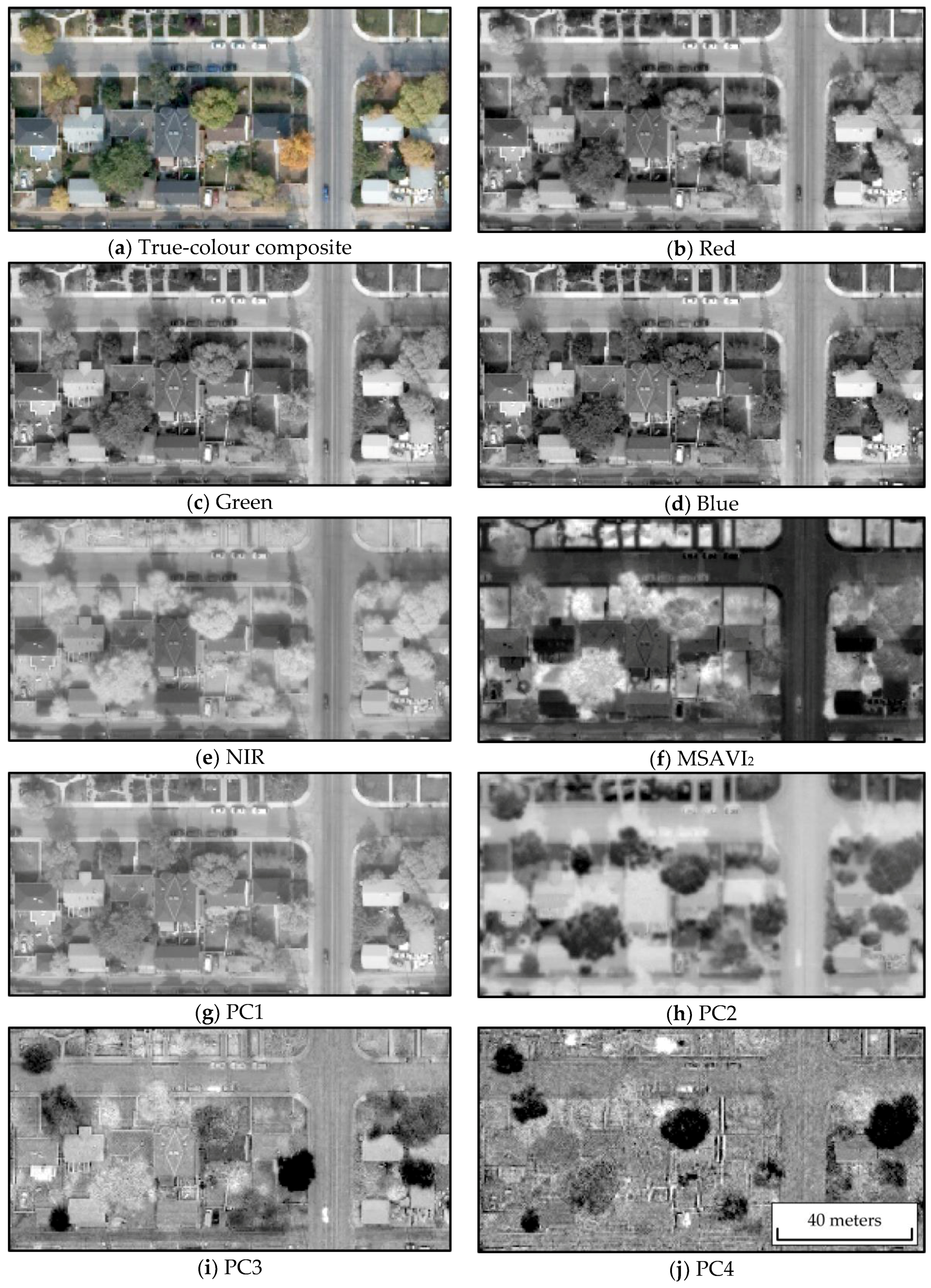
The first principal component (PC1) contained most of the variability in the input dataset with decreasing amounts accounted for by each subsequent component. Specifically, PC1 accounted for most of the variance in the RGBi imagery at 82.9%. PC2 accounted for 16.0% and PC3 and PC4 account for less than 1% each. Typically, the higher PC images are very ‘noisy’; however, in this case PC3 and PC4 visually revealed valuable roof/vegetation information. Table 1 presents the total and cumulative variances as well as the factor loadings, which describe the contributions of each input band to each output principal component. PC1 contains approximately equal amounts of information from the visible bands and a small amount from the NIR band. PC2 primarily contains information from the NIR band, PC3 primarily contains information from the red and blue bands, and PC4 primarily contains information from the green band. Figure 3 presents examples of the RGBi and derived bands for a portion of the study area.

2.6. Segmentation

Prior to segmentation in ENVI FX, we applied a 3 × 3 median filter (edge-preserving) to all nine input raster datasets (RGBi, MSAVI2, PC1–PC4). The intent of this filtering was to reduce the number of small image-objects in the segmentation results, while maintaining the edges of larger discrete image-objects (i.e., rooftop objects).
ENVI FX performs a segmentation operation in two steps: (1) segmentation and (2) merging, each of which can use one or more bands as input. We note that operationally, segmentation is based on a watershed algorithm that operates on a single band to group pixels into an initial set of segments [55]. However, to use multiple input bands from which a single watershed image is created, ENVI FX implements two options: (1) the Edge Method results in a gradient image (via the Sobel edge detector) that is best suited for segmentation of discrete objects; and (2) the Intensity Method computes an across-band average that is better suited for segmentation of continuous fields [55]. After the watershed segmentation, the merging process combines adjacent segments based on a measure of their spectral similarity and shared border length [56]. Merging is an iterative process and produces a set of image-objects that are visually more meaningful than the input set of segments. ENVI FX provides two options for computing the measure of spectral similarity and shared border length (Full Lambda Schedule and Fast Lambda) that implement similar distance functions [56].
Based on visual assessments of trial segmentations, we determined that the MSAVI2, PC2, and PC3 bands were the most suitable inputs for both segmentation and merging. Specifically, we used the Edge Method for segmenting and the Full Lambda Schedule method for merging. In this case, the relevant hyperparameter values were heuristically optimized based on visual assessment (Scale Level = 91 and Merge Level = 36).
Some studies have used vector data directly in the segmentation process [57]. In this case the OSM data for Calgary was too coarse to be useful. It is, however, expected that recent developments in very deep convolutional neural networks will lead to a great increase in the fine scale features present in OSM. See [58] for a recent example of building footprint generation at a very large scale (i.e., the entire contiguous United States) with deep convolutional neural networks.

2.7. Attribute Calculation

ENVI FX can generate 8 attributes based on the DN values of each image-object in each input band and an additional 14 attributes based on the shape of each image-object (Table 2). To fully evaluate this functionality, we computed all attributes for each of the 9 bands resulting in a total of 86 attributes for each image-object. In the following sections, the term “features” refers to the subset of image-object attributes used for classification.

2.8. Pre-Classification Filtering

We used OSM data as ancillary data to exclude image-objects that could be confidently defined as irrelevant classes (i.e., any classes not required to produce the VOR map). For example, any image-objects located away from residential buildings could theoretically be excluded. In practice, we excluded image-objects that (1) represent roads (based on the observation that residential buildings have a minimum, non-zero setback from roads) and (2) fall within an area with a LULC class unlikely to contain residential buildings (e.g., school grounds). The specific OSM element types used are presented with the results in Section 3.1. Generally, filtering was achieved by using ArcGIS to establish a selection of image-objects, using one or more applications of the Select by Location and Select by Attribute tools, then removing the selected image-objects from the dataset.

2.9. Sampling and Response Design

We used image-objects as the primitive units for both classifier training and accuracy assessment. Simple random sampling was used to select 0.25% of the total number of image-objects for use as reference data, as recommended by Thanh Noi and Kappas [61]. The reference image-objects were manually labelled according to our classification scheme. Our scheme was informed by a review of the reference data samples and was established to meet the three criteria noted by Congalton and Green [19], namely that it be (i) mutually exclusive, (ii) exhaustive, and (iii) hierarchical. The properties of being mutually exclusive and having hierarchy are important to allow the classes to be merged into a simple vegetation mask. Consequently, we created nine detailed classes that can be merged into two simplified classes to generate a final veg/non-veg mask (Table 3).
For many of the image-objects, the RGBi and MSAVI2 imagery was sufficient for a confident evaluation of the appropriate class label. For more challenging image-objects, we also considered the higher resolution Google Earth Pro imagery. We note that in VHR imagery of urban areas, shadows become unique objects. As such, there are three detailed vegetation classes: (i) healthy vegetation, (ii) senescing vegetation, and (iii) shadowed vegetation. Also, due to the complex and heterogeneous nature of this detailed urban scene, we note that some rare scene-objects in the reference data were only seen a couple of times. For example, the following scene-objects were represented in the sampled reference image-objects: tennis court surface (n = 1), yellow school buses (n = 1), and construction materials/building under construction (n = 6). In such cases, these image-objects were appropriately labelled as bright impervious surfaces or dark impervious surfaces. Some of the (randomly selected) reference image-objects also represented multiple land cover classes (i.e., mixed-objects). Where mixed-objects were the result of under-segmentation, they were labelled with the majority class. Mixed-objects that represented a mixture of land cover classes but appeared uniform were also observed (e.g., sparse vegetation overhanging a paved road). In these cases, classification was based on an estimate of the dominant class.

2.10. Classification and Accuracy Assessment

For the classification of the image-objects into the nine detailed vegetation and non-vegetation classes, we randomly split the reference data into two portions: a training portion used for model selection and a testing portion used for accuracy assessment. The split was stratified to maintain class proportions in both groups. The sample sizes of the training and testing groups are listed in Section 3. In this study, classification consisted of two steps: (1) model selection, which involved iteratively training many classifiers with different hyperparameters to identify the most suitable hyperparameter values (i.e., hyperparameter tuning), and (2) prediction, which used the selected model to predict class labels for unknown image-objects. Classifier training is performed many times but requires much less computation than prediction because it considers only a (relatively) small training sample of the total number of image-objects. Prediction is more computationally expensive, as it is performed on every image-object; however, it is only done once.
ENVI’s built-in classification tools combine classifier training and prediction into a single step. This makes ENVI inefficient for model selection as each classifier training iteration would also include an unnecessary prediction step. To overcome this limitation, we used Scikit-learn (0.19.1) [62], an open source machine learning library for Python, as it allows training and prediction to be performed separately. Scikit-learn includes implementations of various algorithms for supervised classification (including SVM), unsupervised classification (i.e., clustering), and regression.
SVM models usually map feature vectors to higher dimensional feature space, by means of a kernel function, before computing the optimal hyperplane that separates the classes [63]. Radial Basis Function (RBF) and linear kernels are common. An SVM model with an RBF kernel has two hyperparameters: C , which controls the cost of misclassification in the model, and γ, which controls the width of the kernel (i.e., the spread of the underlying gaussian function). As the linear kernel is just a specific case of the RBF kernel (i.e., where γ ) [64], we did not consider a linear kernel separately. Therefore, following [65], we tuned the model hyperparameters using a simple exhaustive grid search of exponentially increasing values (C = 2−1, 20, …, 29 and γ = 2−6, 2−5, …, 23) and 5-fold cross-validation. The selected hyperparameters were the pair that yielded the highest overall average cross-validation accuracy (based on the training portion of the reference data).
To allow our hypothesis (that a wide range of attributes is important for the successful identification of VOR) to be tested, we evaluate the performance of one model, trained on a comprehensive set of 86 attributes, against a second model, trained on a set of 9 attributes derived only from image-object spectral means. Model selection was performed independently for each model (hereafter referred to as M86 and M9—see Section 3.2.1 for details), then we predicted the detailed classes for the remaining image-objects, finally comparing their classification results.
To understand classification accuracies in the context of VOR, we assessed the predicted classes of test image-objects that overlapped the rooftop polygons. Image-objects were included in the assessment if they intersected rooftop polygons by an area of at least 0.25 m2 (i.e., equivalent to the area of 1 pixel). In addition to this over-rooftop assessment we conducted a full-scene assessment that considered all test image-objects. This additional assessment allowed characterization of over-rooftop accuracy in the context of the accuracy of the entire scene.
For each model, we generated confusion matrices for both the detailed and simplified classes and computed standard accuracy measures and their variances (i.e., overall accuracy, producer’s accuracies, and user’s accuracies). Accuracy assessment calculations were performed using the online thematic Map Accuracy Tools by Salk et al. [66] (see Section 3.2).
To test our hypothesis, we compared the classes predicted for the test image objects by M86 and M9 (considering the simplified classes). We note that the samples were not independent because we used the same single set of test data to evaluate each model. Accordingly, we used McNemar’s test [67] of marginal homogeneity, which is suitable for use with correlated samples. With McNemar’s test, the null hypothesis is that the accuracies are equivalent. The McNemar statistic, Z 2 , has (for large samples) a chi-squared distribution with one degree of freedom and is computed as follows [67,68]:
Z 2 = ( f 12 f 21 ) 2 f 12 + f 21 ,
where f i j is the number of samples correct in set i and incorrect in set j .

2.11. Map Preparation

To obtain the final VOR map, we used ArcGIS to dissolve the boundaries between adjoining vegetation polygons and intersected the results with the geometrically corrected rooftop polygons (Section 2.4). The resulting map and its LULC accuracies were qualitatively assessed and reported in Section 3.2.

3. Results

3.1. Segmentation, Pre-Classification Filtering, and Reference Data Selection

Segmentation, using the Edge Method and the Full Lambda Schedule (see Section 2.6), yielded 624,684 image-objects in our 23.4 km2 study area. We subsequently filtered these image-objects to exclude roads and those falling within LULC areas not expected to contain residential buildings.
To select road image-objects for removal, we identified nine tags that collectively describe the majority of OSM polyline elements that represent roads (listed in Table 4). We then selected all image-objects intersecting these OSM polyline elements. Due to the presence (in some areas) of vegetation overhanging roads, vegetation image-objects were also present in the selection. It was important to remove vegetation from this selection to avoid filtering out any image-objects that may be vegetation over rooftops. Based on heuristic evaluation, we deselected image-objects with mean DN values in PC2 or PC3 less than 120. We found that these criteria were highly successful for removing vegetation image-objects, though many road image-objects were also removed from the selection.
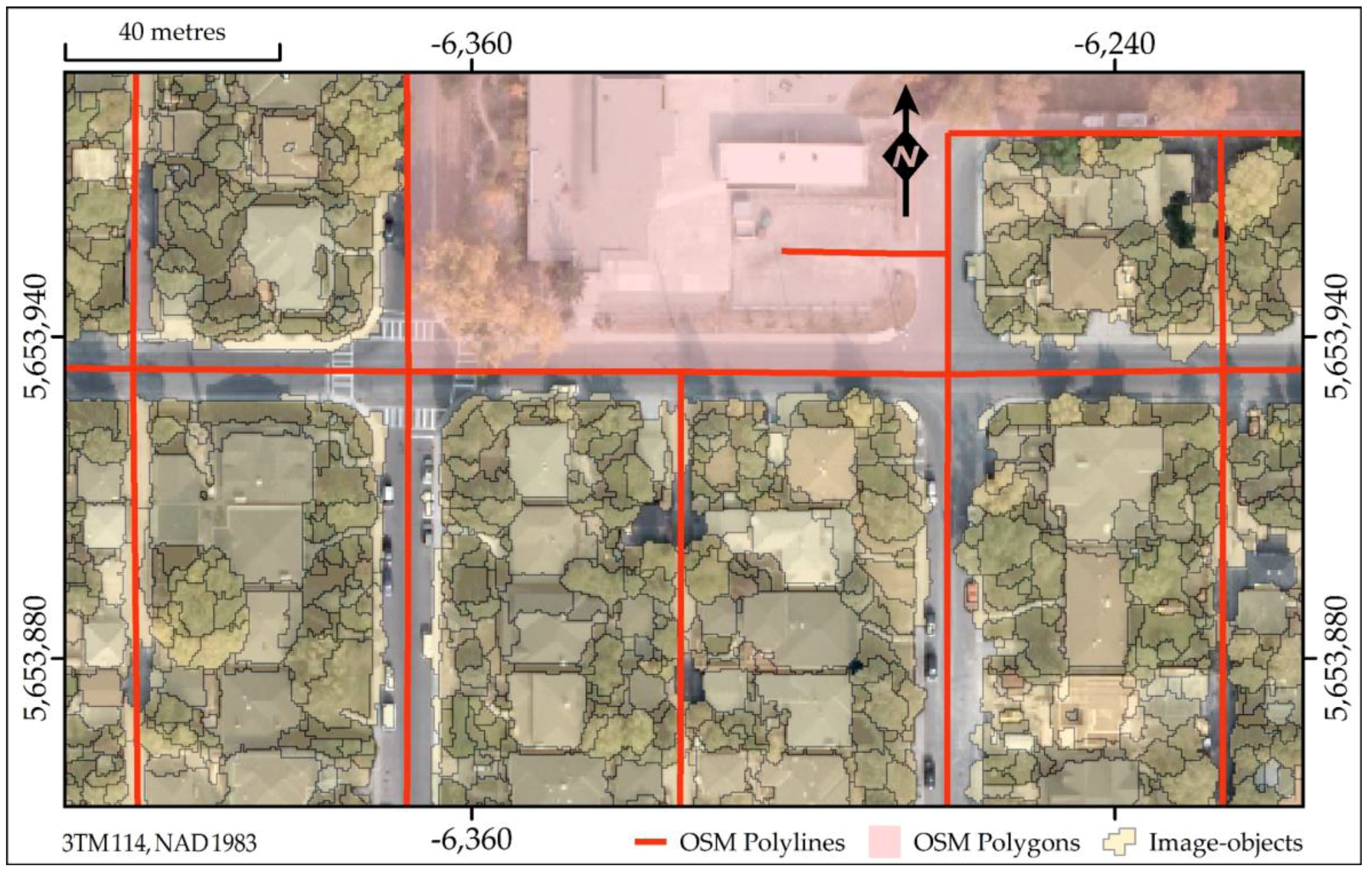
Next, we identified 18 tags describing OSM polygon elements not likely to contain residential buildings (listed in Table 4). We then selected image-objects intersecting these OSM polygon elements and excluded them from the dataset. After pre-classification filtering, our study area contained 537,508 image-objects, representing a 14% reduction. The average size of the filtered image-objects is 106 pixels (26.5 m2) with a standard deviation of 346 pixels (86.5 m2). Figure 4 shows a portion of the study area after pre-classification filtering.
With simple random sampling, we selected 0.25% of the filtered image-objects to be reference data (n = 1344). After manually labelling the reference data, they were randomly split into training and test portions using a 50/50 ratio (stratified to retain the same proportional class distribution as shown in Table 5).

3.2. Model Selection, Classification Accuracy, and Hypothesis Testing

3.2.1. Model Selection

We selected two sets of classification features to compare: (i) all 86 available attributes computed for each image-object and (ii) for each of the 9 bands, only the mean of the DN values within each image-object. A separate SVM model selection was performed for each of the two sets of features, designated M86 (all attributes as features; n = 86) and M9 (mean DN values as features; n = 9). Model selection was performed using the training image-objects. Radial Basis Function (RBF) kernels were used for both models. For both models we found the optimum C to be 28. The optimum γ was 2−5 for M86 and 2−4 for M9.
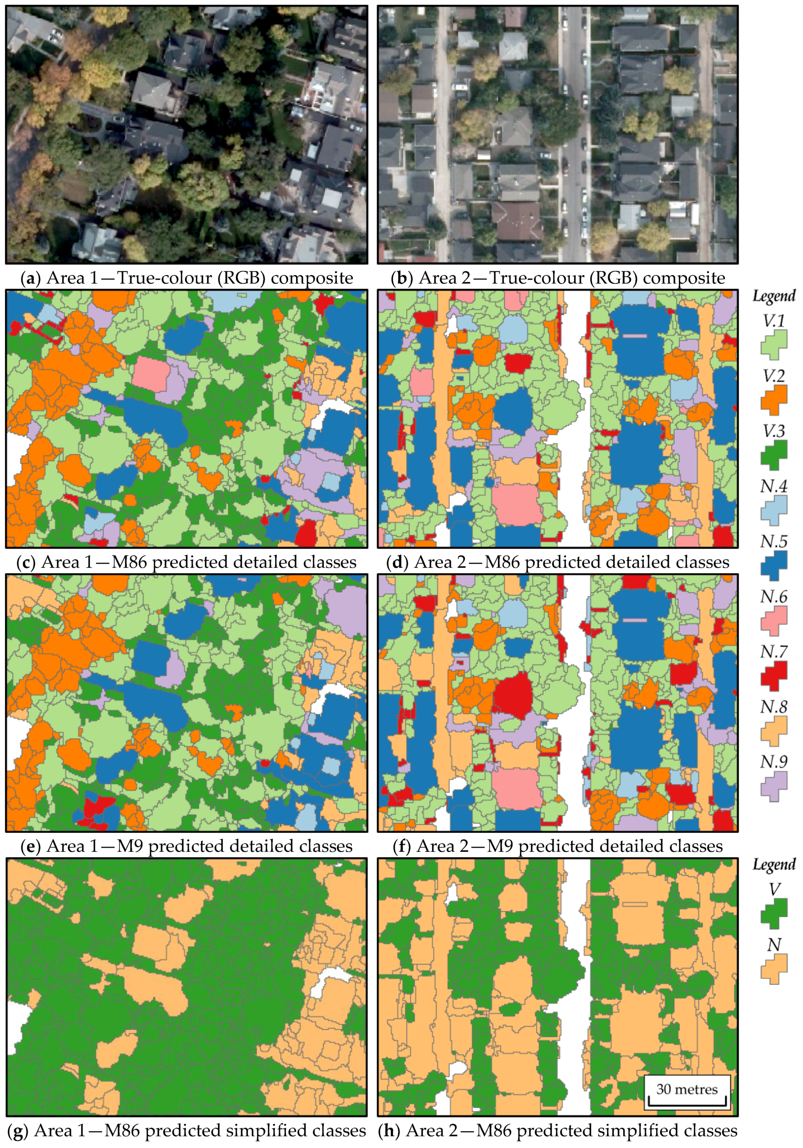
Figure 5 shows two sample areas with examples of detailed classes predicted by M86 and M9 as well as the simplified classes for M86. White regions represent polygons that were not classified by the model, either because they were excluded during pre-classification filtering or because they were reference polygons. The results from M86 and M9 clearly had similar structure; however, they differed from each other in small ways and both included classification errors.
The classification accuracy assessments and the McNemar test were based on evaluation of predicted classes for the test portion of the reference data (n = 672 for the full-scene assessment and n = 122 for the over-rooftop assessment). Confusion matrices were computed for the detailed classes (Table 6 and Table 7) and the simplified classes (Table 8 and Table 9) and provide a detailed accounting of misclassifications. Due to the smaller number of applicable test image-objects, the over-rooftop assessment was only performed on the simplified classes.

3.2.2. Detailed and Simplified Class Accuracies

Predictions from both models showed confusion between the detailed vegetation classes (healthy, senescing, and shadowed)—primarily between healthy (V.1) and senescing (V.2) vegetation. Healthy vegetation had higher producer’s accuracy (81% for both M86 and M9) than senescing vegetation (61% for M86 and 68% for M9). Healthy vegetation also had higher user’s accuracy (83% for M86 and 87% for M9) than senescing vegetation (69% for both M86 and M9). There was also considerable confusion between concrete (N.7) and other bright impervious surfaces (N.8). Similarly, there was notable confusion between the non-rooftop impervious surfaces (N.7, N.8, and N.9) and the vegetation classes (V.1, V.2, and V.3); however, little misclassification occurred between the vegetation and rooftop classes (N.4, N.5, and N.6). Accordingly, the accuracy metrics were generally better for both M86 and M9 after merging into the simplified vegetation (V) and non-vegetation (N) classes. In nearly every case, the producer’s and user’s accuracy were higher for the simplified classes than the detailed classes. Accuracy variances also decreased, particularly for the non-vegetation classes.

3.2.3. Over-Rooftop and Full-Scene Accuracies

A comparison of the overall, producer’s, and user’s accuracies from the over-rooftop assessment and full-scene assessment did not reveal any trend (though accuracy variances were larger for the over-rooftop assessment). The over-rooftop producer’s and user’s accuracies were from 7% lower to 13% higher than the full-scene accuracies. For the M86 model, the producer’s accuracy for vegetation and the user’s accuracy for non-vegetation were higher in the over-rooftop assessment, while for the M9 model, only user’s accuracy for non-vegetation was higher. The M86 overall accuracy was 0.9% higher for the over-rooftop assessment and the M9 overall accuracy was 1.7% lower.

3.2.4. Hypothesis Testing

The correspondence between correctly/incorrectly predicted labels by the M86 and M9 models was tested using the McNemar test. We found that the accuracy of the predictions by the M86 and M9 models did not differ significantly. This was true for both the over-rooftop assessment ( Z 2 = 1.14; p-value = 0.29) and the full-scene assessment ( Z 2 = 0.49; p-value = 0.48). As such, we were unable to reject the null hypothesis that a wide range of attributes is important for the successful identification of VOR.

3.2.5. VOR Qualitative Assessment

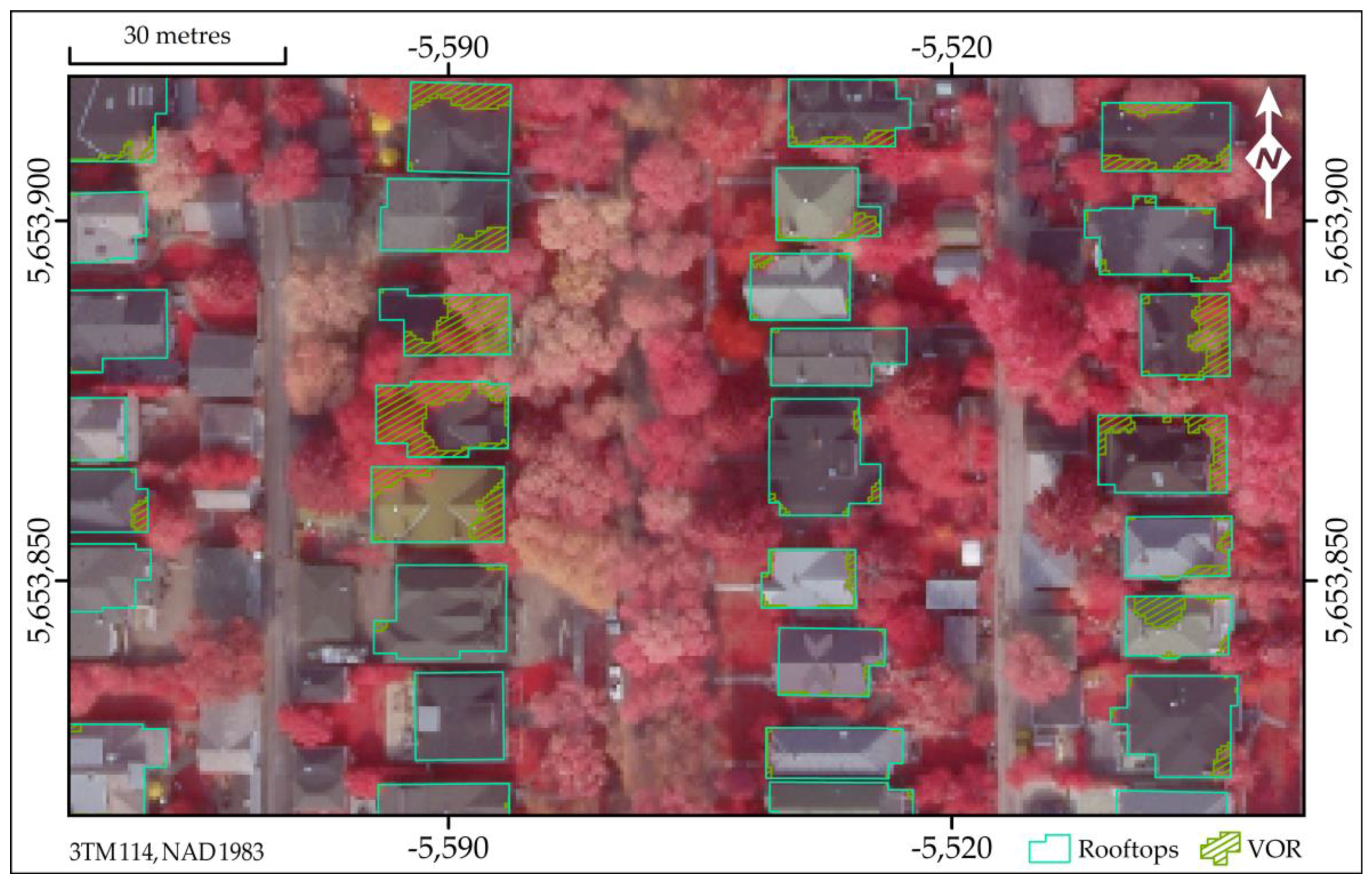
Figure 6 presents a sample of the VOR map shown over a false colour composite (RGB = NIR, red, green). Upon visual assessment, the VOR map appears to successfully mask most of the vegetation over residential rooftops in the study area. Errors of commission appear more common than errors of omission. One example of a commission error, of which multiple instances were observed, is that of dark grey rooftops (N.5) are often classified as deeply shadowed vegetation (V.3). This was observed both for whole rooftops and partial rooftops, such as areas in the shadow of another part of the roof.
Another observation is related to the area along the mask boundaries. In Figure 6, vegetation appears to extend out from under the solid mask, which, at first, puts the positional accuracy of the mask boundaries in question. However, examination of the top panel of Figure 6 reveals vegetation along the inside of the boundary that is darker than the vegetation further from the edge, implying that, like the pixels on the other side of the mask, these pixels represent a combination of the reflectance from the vegetation and the rooftop.

4. Discussion

4.1. Accuracy Assessment

We followed the recommendations of Radoux and Bogaert [69] for the object-based accuracy assessment of wall-to-wall maps, which included calculating overall, producer’s, and user’s accuracies. The accuracy of the classification was based on reference image-objects that were labelled using the source RGBi imagery (0.5 m) supplemented with a higher resolution RGB image (0.2 m), a practice that, while faster and allowing many more image-objects to be used for training and testing, may have been less accurate than labelling based on field visits. As noted by Stehman [70], labelling errors in the reference data reduce the quality of the accuracy assessment.
Based on McNemar’s test of marginal homogeneity, the prediction accuracy of the models was not significantly different. However, the aim of the VOR maps is to ensure vegetation is excluded when determining rooftop emissivity corrections for high-resolution TIR imagery. This means that there is a need to be confident that, if a location is identified as not vegetation on the map, vegetation is indeed not present at the associated position on the ground. As such, it is the user’s accuracies that are the most relevant.
The M9 model consistently had the same or better user’s accuracies for the detailed non-vegetation classes than the M86 model. They were, however, both generally poor, with none of the detailed classes being greater than 50%. This was due in part to confusion between the various non-vegetation classes. The user’s accuracies for the non-vegetation classes improved to 82% (full-scene) and 95% (over-rooftops) when aggregated to the simplified classes. The user’s accuracy for the detailed vegetation classes were generally much higher than the non-vegetation classes and changed less on aggregation into the simplified classes.
Also of note is that the classification accuracy for the full-scene was generally similar to that for the subset of image-objects extending over rooftops. This suggests that considering vegetation over rooftops as a special type of urban vegetation is not necessary for classification purposes (other than the fact that ‘over rooftops’ represents a spatial subset of the full-scene).
An enhanced segmentation validation may be considered for future projects, though it would require a more detailed set of reference data (e.g., independent reference polygons not selected from the segmented image-objects). With such a set of independent reference data, accuracy assessment methods designed for object extraction [71] could be used. An additional limitation of the accuracy assessment is the lack of a field assessment of classification and segmentation accuracy due to funding limitations and the high cost of field validation data. Additionally, future projects will incorporate rooftop delineation methods directly from the remotely sensed data to eliminate the need for an external building polygon dataset.

4.2. Feature Selection and Pre-Classification Filtering

We hypothesized that the additional image-object-specific features available when performing a GEOBIA classification (e.g., ENVI’s texture and spatial attributes) would be important for the successful identification of vegetation over rooftops (VOR). However, the lack of a statistically significant difference between the accuracy of the predicted classes by M86 and M9 indicate that the wide range of additional features beyond spectral means were not necessary for a successful image classification and preparation of an VOR map. This may be explained in part because the specific size and shape of individual image-objects implicitly contain useful spatial information that is spectrally integrated within the mean DN values of each object. As Marceau et al. [72] noted, 90% of the spectral variability of Grey Level Co-occurrence Texture measures was defined by the kernel size. In this case, as previously noted by Hay et al. [73] image-object boundaries represent unique object-specific texture kernels, that contain relevant spatial and spectral information.
Shadows can pose considerable issues for segmentation and classification of trees in high resolution imagery [34]. An issue of interest for this study results from the fact that the degree of light transmittance to the shaded land cover depends on the nature of the occluding object. Buildings, (solid) fences, and other artificial structures will generally absorb or reflect all the light in the wavelengths of available data bands. In contrast, trees will tend to transmit some NIR light and much less visible light, and the degree of transmittance will depend on a number of factors such as the canopy thickness [74]. This means that, for shaded areas of a given land cover type, computed vegetation indices will have different values based on the cause of the shadow, which becomes increasingly complex at very high spatial resolutions. Our imagery also contains senescing vegetation further limiting the utility of common multispectral vegetation indices. However, the high accuracy of the final merged vegetation mask indicates that these issues were sufficiently mitigated.
Pre-classification filtering with the VGI data allowed for a reduction in the number of image-objects to be classified. While no detrimental effect on the classification accuracy was observed from the removal of these image-objects, further study is required to confirm that the classification accuracy was not impacted and to identify additional criteria that may be suitable for pre-classification filtering.

4.3. Fuzzy Vegetation and Heterogeneous Classes

In the context of remote sensing, trees are fuzzy objects [75]. As a result, the boundary defined by the transition between areas of VOR and areas of rooftop is gradual. Despite this fact, the segmentation algorithm appears to have found a reasonable compromise in establishing the hard boundary that represents this transition. For example, the bottom panel of Figure 6 shows that vegetation, mostly appearing red in the false colour composite (RGB = NIR, red, green), appears to extend a few pixels out from beneath the vegetation mask in some areas. However, considering the case where the mask is inverted, we notice that the vegetation tends to appear less dense for the first few pixels inside the mask (i.e., a portion of the rooftop shows through the vegetation). This visual balance indicates that the hard boundaries of the vegetation mask are reasonable. However, moving forward, a specific buffer analysis one pixel wide on either side of the vegetation/rooftop mask boundary combined with a dynamic threshold based on each buffer’s contents [76] is anticipated to further mitigate this issue, though doing so is beyond the scope of this paper.
Reasonably well-defined boundaries between VOR and rooftop areas also highlight the importance of using suitable bands, not only for the classification, but for the initial segmentation. We note that the use of PC2, which discriminated between green vegetation and rooftops (see Panel (h) in Figure 3) and PC3, which discriminated between senescing vegetation and rooftops (see Panel (i) in Figure 3), allowed the segmentation algorithm to establish reasonable boundaries between both healthy and senescing vegetation and rooftops.

5. Conclusions

The availability of very high spatial resolution imagery and appropriate algorithms for its classification has allowed researchers to ask specific very questions about urban vegetation, and do so with high spatial precision. This study examined the specific question of mapping vegetation (trees) that extends out over rooftops in urban areas using passive high resolution airborne imagery. We showed that a combination of a GEOBIA (Geographic Object-Based Image Analysis) classification approach, pre-classification data filtering, and a machine learning classifier were able to generate accurate vegetation masks from very high-resolution RGBi imagery adequate for VOR mapping, despite a complex high-resolution urban environment with deep shadows and senescing vegetation.
In contrast to our initial hypothesis, we found that classification of image-objects using M86, comprising a wide range of spectral, texture, and spatial attributes, did not yield a significantly higher overall classification accuracy (91.8%) than classification using M9, which was based on a smaller number of only spectral attributes (88.5%); a finding which we attribute to spatial information being inherently integrated with the spectral response of well-defined image-objects. The user’s accuracies of the image-object classification are important measures of the suitability of the models for future use in refining rooftop emissivity corrections for high-resolution TIR (thermal infrared) imagery. Our method resulted in balanced user’s accuracies of 89% for vegetation and 88% for non-vegetation based on the simpler M9 model.
We used high-resolution airborne RGBi imagery as the primary input for generating the VOR map, as RGBi imagery is among the most common remote sensing data available from municipalities. We supplemented this with freely available VGI (Volunteered Geographic Information) data from OpenStreetMap. Pre-classification filtering with these VGI data allowed for a 14% reduction in the number of image-objects to be classified without apparent impact on the resulting VOR maps. Data reduction through filtering remains an important consideration for classification as the increasing resolution of imagery results in ever larger volumes of data to process.
The use of bands that maximize the separability between the different types of vegetation and rooftops in the segmentation steps resulted in well positioned boundaries between VOR areas and rooftops in the final map, despite the gradual nature of the transition between VOR and rooftops. As another component of this study, we reviewed the role of remote sensing in urban vegetation mapping and summarized the types of urban vegetation maps generated from these data sources as well as the classification algorithms used to create such maps.

Author Contributions

D.C.G. conceived the study, performed the investigation, and wrote the manuscript. G.J.H. provided supervision, data and reviewed and edited the manuscript.

Funding

This research was based on initial funding received by G.J. Hay as part of a University of Calgary Research Sub-grant of the Alberta Grant on Energy System Analysis pertaining to Program Element 4, entitled ‘Modeling and Analysis of Energy System Components’.

Acknowledgments

OpenStreetMap data © OpenStreetMap contributors and available from www.openstreetmap.org under the Open Database License, “ODbL” 1.0. Figure 1 base data obtained from Open Calgary (data.calgary.ca) and Natural Earth (www.naturalearthdata.com). Figure 5 colour palette from Color Brewer 2.0 (http://colorbrewer2.org).

Conflicts of Interest

The authors declare no conflict of interest.

Abbreviations

DASDigital Aerial Survey
DNDigital Number
DTDecision Tree
GEOBIAGeographic Object-Based Image Analysis
kNNk-Nearest Neighbour
LiDARLight Detection and Ranging
LULCLand-Use and Land-Cover
MSAVIModified Soil-Adjusted Vegetation Index
MSSMultispectral Scanner
NDVINormalized Difference Vegetation Index
NIRNear-Infrared
OSMOpenStreetMap
PCPrincipal Component
RBFRadial Basis Function
RGBRed, Green, and Blue
RGBiRed, Green, Blue, and near-infrared
SAVISoil-Adjusted Vegetation Index
SVMSupport Vector Machine
TIRThermal Infrared
VGIVolunteered Geographic Information
VHRVery High Resolution
VORVegetation Over Rooftops

References

  1. Roy, S.; Byrne, J.; Pickering, C. A systematic quantitative review of urban tree benefits, costs, and assessment methods across cities in different climatic zones. Urban For. Urban Green. 2012, 11, 351–363. [Google Scholar] [CrossRef]
  2. Nowak, D.J.; Crane, D.E.; Stevens, J.C. Air pollution removal by urban trees and shrubs in the United States. Urban For. Urban Green. 2006, 4, 115–123. [Google Scholar] [CrossRef] [Green Version]
  3. Armson, D.; Ennos, A.R.; Stringer, P. The effect of tree shade and grass on surface and globe temperatures in an urban area. Urban For. Urban Green. 2012, 11, 245–255. [Google Scholar] [CrossRef]
  4. Livesley, S.J.; Baudinette, B.; Glover, D. Rainfall interception and stem flow by eucalypt street trees–The impacts of canopy density and bark type. Urban For. Urban Green. 2014, 13, 192–197. [Google Scholar] [CrossRef]
  5. Song, X.P.; Tan, P.Y.; Edwards, P.; Richards, D. The economic benefits and costs of trees in urban forest stewardship: A systematic review. Urban For. Urban Green. 2018, 29, 162–170. [Google Scholar] [CrossRef]
  6. Nyberg, R.; Johansson, M. Indicators of road network vulnerability to storm-felled trees. Nat. Hazards 2013, 69, 185–199. [Google Scholar] [CrossRef]
  7. Jacbos, B.; Mikhailovich, N.; Delaney, C. Benchmarking Australia’s Urban Tree Canopy: An i-Tree Assessment; Final Report; University of Technology Sydney: Sydney, Australia, 2014. [Google Scholar]
  8. Ordóñez, C.; Duinker, P.N. Assessing the vulnerability of urban forests to climate change. Environ. Rev. 2014, 22, 311–321. [Google Scholar] [CrossRef]
  9. Brandt, L.; Lewis, A.D.; Fahey, R.; Scott, L.; Darling, L.; Swanston, C. A framework for adapting urban forests to climate change. Environ. Sci. Policy 2016, 66, 393–402. [Google Scholar] [CrossRef]
  10. Gill, S.E.; Handley, J.F.; Ennos, A.R.; Pauleit, S. Adapting cities for climate change: The role of the green infrastructure. Built. Environ. 2007, 33, 115–133. [Google Scholar] [CrossRef]
  11. Fogl, M.; Moudrý, V. Influence of vegetation canopies on solar potential in urban environments. Appl. Geogr. 2016, 66, 73–80. [Google Scholar] [CrossRef]
  12. Hemachandran, B. Developing HEAT Scores with h-Res Thermal Imagery to Support Urban Energy Efficiency. Master’s Thesis, University of Calgary, Calgary, AB, Canada, 2013, unpublished. [Google Scholar]
  13. Zhao, Q.; Myint, S.W.; Wentz, E.A.; Fan, C. Rooftop surface temperature analysis in an urban residential environment. Remote Sens. 2015, 7, 12135–12159. [Google Scholar] [CrossRef]
  14. Hay, G.J.; Kyle, C.; Hemachandran, B.; Chen, G.; Rahman, M.M.; Fung, T.S.; Arvai, J.L. Geospatial technologies to improve urban energy efficiency. Remote Sens. 2011, 3, 1380–1405. [Google Scholar] [CrossRef]
  15. Nichol, J. An emissivity modulation method for spatial enhancement of thermal satellite images in urban heat island analysis. Photogramm. Eng. Remote Sens. 2009, 75, 547–556. [Google Scholar] [CrossRef]
  16. The City of Calgary. 2014 September Snow Storm & Tree Debris Clean up. Available online: http://www.calgary.ca/CSPS/Parks/Documents/History/Conserving-Calgarys-Historic-Streets-Plan.pdf (accessed on 10 November 2018). (Archived by WebCite® at http://www.webcitation.org/73qB7uKFG).
  17. Pu, R.; Landry, S. A comparative analysis of high spatial resolution IKONOS and WorldView-2 imagery for mapping urban tree species. Remote Sens. Environ. 2012, 124, 516–533. [Google Scholar] [CrossRef]
  18. Tigges, J.; Lakes, T.; Hostert, P. Urban vegetation classification: Benefits of multitemporal RapidEye satellite data. Remote Sens. Environ. 2013, 136, 66–75. [Google Scholar] [CrossRef]
  19. Congalton, R.G.; Green, K. Assessing the Accuracy of Remotely Sensed Data: Principles and Practices, 2nd ed.; CRC Press: Boca Raton, FL, USA, 2009; ISBN 978-1-4200-5512-2. [Google Scholar]
  20. Myeong, S.; Nowak, D.J.; Hopkins, P.F.; Brock, R.H. Urban cover mapping using digital, high-spatial resolution aerial imagery. Urban Ecosyst. 2001, 5, 243–256. [Google Scholar] [CrossRef]
  21. Mathieu, R.; Aryal, J.; Chong, A.K. Object-based classification of IKONOS imagery for mapping large-scale vegetation communities in urban areas. Sensors 2007, 7, 2860–2880. [Google Scholar] [CrossRef] [PubMed]
  22. Agarwal, S.; Vailshery, L.; Jaganmohan, M.; Nagendra, H. Mapping urban tree species using very high resolution satellite imagery: Comparing pixel-based and object-based approaches. ISPRS Int. J. Geo-Inf. 2013, 2, 220–236. [Google Scholar] [CrossRef]
  23. Nielsen, A.B.; Östberg, J.; Delshammar, T. Review of urban tree inventory methods used to collect data at single-tree level. Arboric. Urban For. 2014, 40, 96–111. [Google Scholar]
  24. Blaschke, T.; Hay, G.J.; Weng, Q.; Resch, B. Collective sensing: Integrating geospatial technologies to understand urban systems—An overview. Remote Sens. 2011, 3, 1743–1776. [Google Scholar] [CrossRef]
  25. Jensen, J.R. Introductory Digital Image Processing: A Remote Sensing Perspective; Always Learning; Pearson Education: London, UK, 2016; ISBN 9780134058160. [Google Scholar]
  26. Abdulkarim, B.; Kamberov, R.; Hay, G.J. Supporting urban energy efficiency with volunteered roof information and the Google Maps API. Remote Sens. 2014, 6, 9691–9711. [Google Scholar] [CrossRef]
  27. Zhang, X.; Feng, X.; Jiang, H. Object-oriented method for urban vegetation mapping using IKONOS imagery. Int. J. Remote Sens. 2010, 31, 177–196. [Google Scholar] [CrossRef]
  28. Yang, T.L. Mapping vegetation in an urban area with stratified classification and multiple endmember spectral mixture analysis. Remote Sens. Environ. 2013, 133, 251–264. [Google Scholar] [CrossRef]
  29. Wen, D.; Huang, X.; Liu, H.; Liao, W.; Zhang, L. Semantic classification of urban trees using very high resolution satellite imagery. IEEE J. Sel. Top. Appl. Earth Obs. Remote Sens. 2017, 10, 1413–1424. [Google Scholar] [CrossRef]
  30. Jensen, J.R.; Im, J.; Hardin, P.; Jensen, R.R. Image Classification. In The SAGE Handbook of Remote Sensing; SAGE Publications, Ltd.: London, UK, 2009; pp. 269–281. ISBN 9780857021052. [Google Scholar]
  31. Moskal, L.M.; Styers, D.M.; Halabisky, M. Monitoring urban tree cover using object-based image analysis and public domain remotely sensed data. Remote Sens. 2011, 3, 2243–2262. [Google Scholar] [CrossRef]
  32. Walker, J.S.; Briggs, J.M. An object-oriented approach to urban forest mapping in Phoenix. Photogramm. Eng. Remote Sens. 2007, 73, 577–583. [Google Scholar] [CrossRef]
  33. Belgiu, M.; Drăguţ, L. Random forest in remote sensing: A review of applications and future directions. ISPRS J. Photogramm. Remote Sens. 2016, 114, 24–31. [Google Scholar] [CrossRef]
  34. Zhang, K.; Hu, B. Individual urban tree species classification using very high spatial resolution airborne multi-spectral imagery using longitudinal profiles. Remote Sens. 2012, 4, 1741–1757. [Google Scholar] [CrossRef]
  35. Feng, Q.; Liu, J.; Gong, J. UAV remote sensing for urban vegetation mapping using random forest and texture analysis. Remote Sens. 2015, 7, 1074–1094. [Google Scholar] [CrossRef]
  36. Iovan, C.; Boldo, D.; Cord, M. Detection, characterization, and modeling vegetation in urban areas from high-resolution aerial imagery. IEEE J. Sel. Top. Appl. Earth Obs. Remote Sens. 2008, 1, 206–213. [Google Scholar] [CrossRef]
  37. Chen, G.; Hay, G.J. A support vector regression approach to estimate forest biophysical parameters at the object level using airborne LiDAR transects and QuickBird data. Photogramm. Eng. Remote Sens. 2011, 77, 733–741. [Google Scholar] [CrossRef]
  38. Mountrakis, G.; Im, J.; Ogole, C. Support vector machines in remote sensing: A review. ISPRS J. Photogramm. Remote Sens. 2011, 66, 247–259. [Google Scholar] [CrossRef]
  39. Welch, R. Spatial resolution requirements for urban studies. Int. J. Remote Sens. 1982, 3, 139–146. [Google Scholar] [CrossRef]
  40. Jensen, J.; Cowen, D. Remote sensing of urban/suburban infrastructure and socio-economic attributes. Photogramm. Eng. Remote Sens. 1999, 65, 611–622. [Google Scholar]
  41. Myint, S.W.; Gober, P.; Brazel, A.; Grossman-Clarke, S.; Weng, Q. Per-pixel vs. object-based classification of urban land cover extraction using high spatial resolution imagery. Remote Sens. Environ. 2011, 115, 1145–1161. [Google Scholar] [CrossRef]
  42. Hay, G.J.; Castilla, G. Geographic Object-Based Image Analysis (GEOBIA): A new name for a new discipline. In Object-Based Image Analysis: Spatial Concepts for Knowledge-Driven Remote Sensing Applications; Blaschke, T., Lang, S., Hay, G.J., Eds.; Lecture Notes in Geoinformation and Cartography; Springer: Berlin/Heidelberg, Germany, 2008; pp. 75–89. ISBN 978-3-540-77058-9. [Google Scholar]
  43. Ke, Y.; Quackenbush, L.J. A review of methods for automatic individual tree-crown detection and delineation from passive remote sensing. Int. J. Remote Sens. 2011, 32, 4725–4747. [Google Scholar] [CrossRef]
  44. Zhen, Z.; Quackenbush, L.J.; Zhang, L. Trends in automatic individual tree crown detection and delineation—Evolution of LiDAR data. Remote Sens. 2016, 8, 333. [Google Scholar] [CrossRef]
  45. Fassnacht, F.E.; Latifi, H.; Stereńczak, K.; Modzelewska, A.; Lefsky, M.; Waser, L.T.; Straub, C.; Ghosh, A. Review of studies on tree species classification from remotely sensed data. Remote Sens. Environ. 2016, 186, 64–87. [Google Scholar] [CrossRef]
  46. The City of Calgary. Conserving Calgary’s Historic Streets: A Conservation Plan for 27 of Calgary’s Historic Streetscapes. Available online: http://www.calgary.ca/CSPS/Parks/Documents/History/Conserving-Calgarys-Historic-Streets-Plan.pdf (accessed on 13 September 2018).
  47. The City of Calgary. Urban Forest Management. Available online: https://maps.calgary.ca/TreeSchedule/ (accessed on 13 September 2018).
  48. The City of Calgary. History of Annexation. Available online: http://www.calgary.ca/PDA/pd/Documents/pdf/history-of-annexation.pdf (accessed on 13 September 2018).
  49. The City of Calgary. Digital Aerial Survey. Available online: http://www.calgary.ca/CS/IIS/Pages/Mapping-products/Digital-Aerial-Survey.aspx (accessed on 13 September 2018). (Archived by WebCite® at http://www.webcitation.org/71yZ8TSDM).
  50. Holtkamp, D.J.; Goshtasby, A.A. Precision registration and mosaicking of multicamera images. IEEE Trans. Geosci. Remote Sens. 2009, 47, 3446–3455. [Google Scholar] [CrossRef]
  51. Huete, A.R. A soil-adjusted vegetation index (SAVI). Remote Sens. Environ. 1988, 25, 295–309. [Google Scholar] [CrossRef]
  52. Qi, J.; Chehbouni, A.; Huete, A.R.; Kerr, Y.H.; Sorooshian, S. A modified adjusted vegetation index. Remote Sens. Environ. 1994, 48, 119–126. [Google Scholar] [CrossRef]
  53. Kauth, R.J.; Thomas, G.S. The tasselled cap—A graphic description of the spectral-temporal development of agricultural crops as seen by Landsat. In Proceedings of the Symposium on Machine Processing of Remotely Sensed Data, West Lafayette, IN, USA, 29 June–1 July 1976; pp. 41–51. [Google Scholar]
  54. Crist, E.P.; Cicone, R.C. A physically-based transformation of thematic mapper data—The TM tasseled cap. IEEE Trans. Geosci. Remote Sens 1984, GE-22, 256–263. [Google Scholar] [CrossRef]
  55. Harris Geospatial Solutions Inc. Segmentation Algorithms Background. Available online: http://www.harrisgeospatial.com/docs/BackgroundSegmentationAlgorithm.html (accessed on 13 September 2018). (Archived by WebCite® at http://www.webcitation.org/71yX3GhvP).
  56. Harris Geospatial Solutions Inc. Merge Algorithms Background. Available online: http://www.harrisgeospatial.com/docs/BackgroundMergeAlgorithms.html (accessed on 13 September 2018). (Archived by WebCite® at http://www.webcitation.org/71yXkbNa0).
  57. Smith, G.M.; Morton, R.D. Real world objects in GEOBIA through the exploitation of existing digital cartography and image segmentation. Photogramm. Eng. Remote Sens. 2010, 76, 163–171. [Google Scholar] [CrossRef]
  58. Yang, H.L.; Yuan, J.; Lunga, D.; Laverdiere, M.; Rose, A.; Bhaduri, B. Building extraction at scale using convolutional neural network: Mapping of the united states. IEEE J. Sel. Top. Appl. Earth Obs. Remote Sens. 2018, 99, 1–15. [Google Scholar] [CrossRef]
  59. Harris Geospatial Solutions Inc. List of Attributes. Available online: http://www.harrisgeospatial.com/docs/AttributeList.html (accessed on 13 September 2018). (Archived by WebCite® at http://www.webcitation.org/71yXmokmR).
  60. Harris Geospatial Solutions Inc. Texture Metrics Background. Available online: http://www.harrisgeospatial.com/docs/backgroundtexturemetrics.html (accessed on 13 September 2018). (Archived by WebCite® at http://www.webcitation.org/71yXqA6AW).
  61. Thanh Noi, P.; Kappas, M. Comparison of random forest, k-nearest neighbor, and support vector machine classifiers for land cover classification using Sentinel-2 imagery. Sensors. 2018, 18, 18. [Google Scholar] [CrossRef] [PubMed]
  62. Pedregosa, F.; Varoquaux, G.; Gramfort, A.; Michel, V.; Thirion, B.; Grisel, O.; Blondel, M.; Prettenhofer, P.; Weiss, R.; Dubourg, V.; et al. Scikit-learn: Machine learning in Python. J. Mach. Learn. Res. 2011, 12, 2825–2830. [Google Scholar]
  63. Vapnik, V.N.; Chapelle, O. Bounds on error expectation for support vector machines. Neural Comput. 2000, 12, 2013–2036. [Google Scholar] [CrossRef] [PubMed]
  64. Keerthi, S.S.; Lin, C.-J. Asymptotic behaviors of support vector machines with gaussian kernel. Neural Comput. 2003, 15, 1667–1689. [Google Scholar] [CrossRef] [PubMed]
  65. Hsu, C.-W.; Chang, C.-C.; Lin, C.-J. A Practical Guide to Support Vector Classification; National Taiwan University: Taipei, Taiwan, 2003–2016; Available online: https://www.csie.ntu.edu.tw/~cjlin/papers/guide/guide.pdf (accessed on 13 September 2018).
  66. Salk, C.; Fritz, S.; See, L.; Dresel, C.; McCallum, I. An exploration of some pitfalls of thematic map assessment using the new map tools resource. Remote Sens. 2018, 10, 376. [Google Scholar] [CrossRef]
  67. McNemar, Q. Note on the sampling error of the difference between correlated proportions or percentages. Psychometrika 1947, 12, 153–157. [Google Scholar] [CrossRef] [PubMed]
  68. Agresti, A.; Min, Y. Effects and non-effects of paired identical observations in comparing proportions with binary matched-pairs data. Stat. Med. 2004, 23, 65–75. [Google Scholar] [CrossRef] [PubMed]
  69. Radoux, J.; Bogaert, P. Good practices for object-based accuracy assessment. Remote Sens. 2017, 9, 646. [Google Scholar] [CrossRef]
  70. Stehman, S. V Statistical rigor and practical utility in thematic map accuracy assessment. ISPRS J. Photogramm. Remote Sens. 2001, 67, 727–734. [Google Scholar]
  71. Cai, L.; Shi, W.; Miao, Z.; Hao, M. Accuracy assessment measures for object extraction from remote sensing images. Remote Sens. 2018, 10, 303. [Google Scholar] [CrossRef]
  72. Marceau, D.J.; Howarth, P.J.; Dubois, J.M.; Gratton, D.J. Evaluation of the grey-level co-occurrence matrix method for land-cover classification using SPOT imagery. IEEE Trans. Geosci. Remote Sens. 1990, 28, 513–519. [Google Scholar] [CrossRef]
  73. Hay, G.J.; Niemann, K.O.; McLean, G.F. An object-specific image-texture analysis of H-resolution forest imagery. Remote Sens. Environ. 1996, 55, 108–122. [Google Scholar] [CrossRef]
  74. Berard, G.M.; Cloutis, E.A.; Mann, P. Leaf reflectance and transmission properties (350–2500 nm): Implications for vegetation indices. J. Near Infrared Spectrosc. 2017, 25, 138–144. [Google Scholar] [CrossRef]
  75. Ardila, J.P.; Bijker, W.; Tolpekin, V.A.; Stein, A. Quantification of crown changes and change uncertainty of trees in an urban environment. ISPRS J. Photogramm. Remote Sens. 2012, 74, 41–55. [Google Scholar] [CrossRef]
  76. Shorter, N.; Kasparis, T. Automatic vegetation identification and building detection from a single nadir aerial image. Remote Sens. 2009, 1, 731–757. [Google Scholar] [CrossRef]
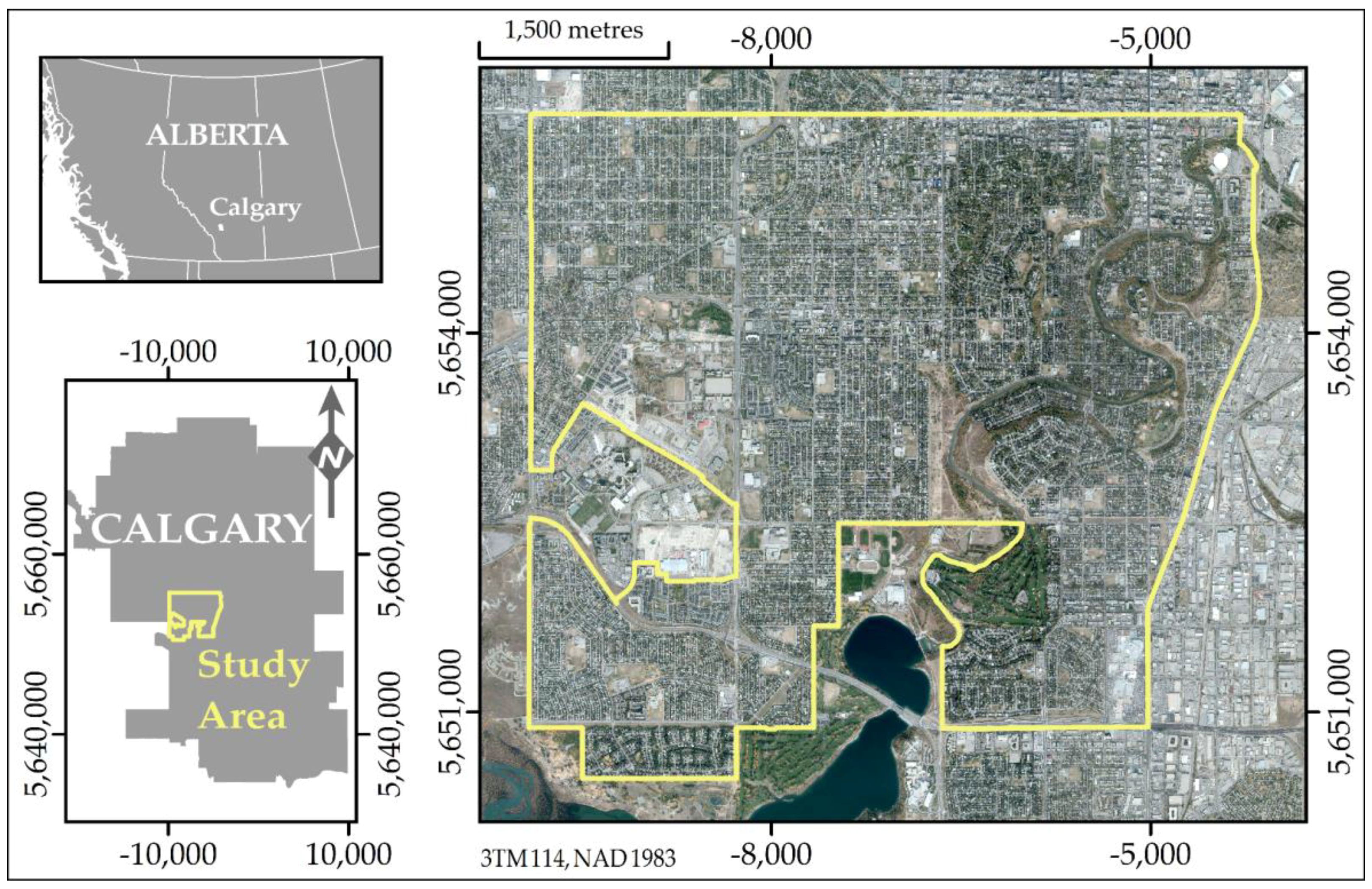
Figure 1. Study area (yellow) located in the City of Calgary, Alberta, Canada, overlaid on a true-colour composite of a four band (RGBi) orthoimage.
Ijgi 07 00462 g001
Figure 2. Flow chart showing the study methodology with details available in the corresponding section numbers (Section 2.4, Section 2.5, Section 2.6, Section 2.7, Section 2.8, Section 2.9, Section 2.10 and Section 2.11). An overview of the methodology is presented in Section 2.3.
Ijgi 07 00462 g002
Figure 3. Sub-section of study area showing rooftops and vegetation in (a) true-colour composite, (be) red, green, blue, and NIR bands, (f) MSAVI2 band, and (gj) PC1-PC4 bands. Visual assessment reveals that a combination of bands MSAVI2, PC2, and PC3 is suitable for differentiating vegetation from rooftops.
Ijgi 07 00462 g003
Figure 4. OpenStreetMap (OSM) data and image-objects (after pre-classification filtering) shown overlaid on a true-color image. Also shown are OSM polylines representing roads (red) and an OSM polygon representing a school ground (pink). Some image-objects intersecting road polylines were not filtered as they have the potential to represent vegetation over rooftops.
Ijgi 07 00462 g004
Figure 5. Classified image-objects for two example areas: Area 1 (left) and Area 2 (right). (a,b) show true-colour ortho-composites. (c,d) show detailed model M86 classes. (e,f) show detailed model M9 classes. (g,h) show simplified M86 classes. V = Vegetation (veg.) and N = Non-veg. V.1 = Healthy veg.; V.2 = Senescing veg.; V.3 = Shadowed veg.; N.4 = Light grey rooftops; N.5 = Dark grey rooftops; N.6 = Red and brown rooftops; N.7 = Concrete; N.8 = Other impervious bright; and N.9 = Other impervious dark. White areas are training, testing, or excluded polygons.
Ijgi 07 00462 g005
Figure 6. Example of vegetation over rooftop (VOR) map based on the M86 model results, with VOR shown as green hatched polygons. Polygons are shown over a false colour composite (RGB = NIR, red, green).
Ijgi 07 00462 g006
Table 1. Individual and cumulative variance accounted for by the principal components of the RGBi imagery, and the RGBi factor loadings for each principal component.
ComponentVarianceBand Contributions (Factor Loadings)
TotalCumulativeRedGreenBlueNIR
PC182.9%82.9%32%27%30%10%
PC216.0%98.9%0%2%12%86%
PC30.9%99.8%61%2%34%3%
PC40.2%100.0%6%69%24%1%
Table 2. Attributes computed by ENVI FX for image-objects.
AttributeType 1Description/Equation 3,4
MeanSpectralMean of values
MaximumSpectralMaximum of values
MinimumSpectralMinimum of values
Standard deviationSpectralStandard deviation of values
RangeTexture 2Average of kernel range values
MeanTexture 2Average of kernel mean values
VarianceTexture 2Average of kernel variance values
EntropyTexture 2Average of kernel entropy values, where
E n t r o p y = i = 0 N g P ( i ) ln P ( i ) (2)
AreaSpatialTotal area within object less area within any holes
LengthSpatialLength of object perimeter and perimeters of any holes
CompactnessSpatial C o m p a c t n e s s = 4 a r e a π o u t e r   c o n t o u r   l e n g t h (3)
ConvexitySpatial C o n v e x i t y = l e n g t h   o f   c o n v e x   h u l l L e n g t h (4)
SoliditySpatial S o l i d i t y = A r e a a r e a   o f   c o n v e x   h u l l (5)
RoundnessSpatial R o u n d n e s s = 4 A r e a π M a j o r   l e n g t h 2 (6)
Form factorSpatial F o r m   f a c t o r = 4 π A r e a t o t a l   p e r i m e t e r 2 (7)
ElongationSpatial E l o n g a t i o n = M a j o r   l e n g t h M i n o r   l e n g t h (8)
Rectangular fitSpatial R e c t a n g u l a r   f i t = A r e a M a j o r   l e n g t h M i n o r   l e n g t h (9)
Main directionSpatialAngle subtended by major axis and x-axis (degrees)
Major lengthSpatialMajor axis length for an oriented bounding box
Minor lengthSpatialMinor axis length for an oriented bounding box
HolesSpatialNumber of holes
Hole solid ratioSpatial H o l e   s o l i d   r a t i o = A r e a o u t e r   c o n t o u r   a r e a (10)
1 ENVI FX groups image-object attributes into three categories: spectral, texture, and spatial. Spectral and texture attributes are computed for each band for each image-object. Spatial attributes are computed only once for each image-object. 2 Each texture attribute is computed in two steps: (1) for each pixel in the image-object the attribute is computed with a centered kernel and (2) the resulting values are averaged. Based on visual assessment, we used an 11 × 11 kernel for texture calculations. 3 Attribute descriptions and equations reproduced from ENVI documentation [59]. 4 N g is the number of unique grey values in the kernel and P ( i ) is the probability of the i th pixel value [60].
Table 3. The classification scheme used is hierarchical with nine detailed classes that can be merged into two simplified classes. At each level, the classes are mutually exclusive and exhaustive. Each class label is assigned a short identifier for clarity, which is shown in parentheses before the class name.
Detailed ClassesSimplified Classes
(V.1) Healthy vegetation(V) Vegetation
(V.2) Senescing vegetation
(V.3) Shadowed vegetation
(N.4) Light grey rooftops(N) Non-vegetation
(N.5) Dark grey rooftops
(N.6) Red and brown rooftops
(N.7) Concrete
(N.8) Other impervious bright
(N.9) Other impervious dark
Table 4. Tags (key = value pairs) for OpenStreetMap (OSM) polyline elements that correspond to city roads and OSM polygon elements unlikely to contain rooftops or vegetation over rooftops (VOR).
Tags for Representing RoadsTags Representing Areas Absent of Rooftops/VOR
KeyValueKeyValueKeyValue
highway =motorwayleisure =parknatural =wood
motorway_link golf_course water
secondary sports_centre scrub
secondary_link pitchlanduse =retail
tertiaryshop =mall recreation_ground
tertiary_linkamenity =parking industrial
service school military
residential clinic cemetery
unclassified 1waterway =riverbank brownfield
1 Visual inspection revealed that the “highway = unclassified” elements were mostly roads.
Table 5. Quantities of training image-objects and test image-objects by class (with related numbers of pixels). These reference data were obtained by simple random sampling of the image-objects rather than point-based sampling to avoid introducing sampling bias (as image-objects are of variable size). Reference data was randomly split into training and test portions (50% each), stratified by class. A subset of the test data was then extracted for evaluation of vegetation overhanging rooftops.
Detailed Class LabelTotal No. of Reference Objects
(# Pixels)
No. of Training Objects
(# Pixels)
No. of Test Objects
(# Pixels)
No. of Over-Rooftop Test Objects
(# Pixels)
(V.1) Healthy vegetation557
(43,709)
278
(20,737)
279
(22,972)
43
(3819)
(V.2) Senescing vegetation237
(23,327)
119
(12,212)
118
(11,115)
14
(1500)
(V.3) Shadowed vegetation97
(8451)
49
(4516)
48
(3935)
7
(762)
(N.4) Light grey rooftops54
(15,213)
27
(6794)
27
(8419)
15
(5063)
(N.5) Dark grey rooftops51
(21,031)
26
(9768)
25
(11,263)
13
(6705)
(N.6) Red and brown rooftops25
(3384)
12
(1417)
13
(1967)
5
(1067)
(N.7) Concrete121
(7943)
60
(4110)
61
(3833)
11
(811)
(N.8) Other impervious bright128
(16,277)
64
(8433)
64
(7844)
8
(1077)
(N.9) Other impervious dark74
(5713)
37
(2935)
37
(2778)
6
(619)
Total1344
(145,048)
672
(74,126)
672
(70,922)
122
(21,423)
Table 6. Confusion matrix and derived accuracy measures for model M86’s predictions of detailed classes for the test data. V.# refer to vegetation classes and N.# refer to non-vegetation classes.
M86—Detailed:Reference Class Labels—Full-Scene
Predicted Class LabelsV.1V.2V.3N.4N.5N.6N.7N.8N.9
(V.1) Healthy vegetation232334010117
(V.2) Senescing vegetation26820000055
(V.3) Shadowed vegetation7041000000
(N.4) Light grey rooftops 0001210851
(N.5) Dark grey rooftops 1200121117
(N.6) Red and brown rooftops 220024111
(N.7) Concrete 45014030152
(N.8) Other impervious bright 7509046303
(N.9) Other impervious dark 6520432213
Producer’s Accuracy81%61%87%55%50%33%61%50%33%
Producer’s Accuracy Variance4%7%9%18%17%24%12%11%13%
User’s Accuracy83%69%85%44%48%31%49%47%35%
User’s Accuracy Variance4%8%10%19%20%26%13%12%16%
Overall Accuracy67.9%
Overall Accuracy Variance3.3%
Table 7. Confusion matrix and derived accuracy measures for model M9’s predictions of detailed classes for the test data. V.# refer to vegetation classes and N.# refer to non-vegetation classes.
M9—Detailed:Reference Class Labels—Full-Scene
Predicted Class LabelsV.1V.2V.3N.4N.5N.6N.7N.8N.9
(V.1) Healthy vegetation243213000606
(V.2) Senescing vegetation27820000234
(V.3) Shadowed vegetation3045000000
(N.4) Light grey rooftops 1001200671
(N.5) Dark grey rooftops 4000100137
(N.6) Red and brown rooftops 110004061
(N.7) Concrete 54043029151
(N.8) Other impervious bright 411011126281
(N.9) Other impervious dark 11210422312
Producer’s Accuracy81%68%92%44%56%50%56%43%36%
Producer’s Accuracy Variance4%7%7%16%21%32%12%10%14%
User’s Accuracy87%69%94%44%40%31%48%44%32%
User’s Accuracy Variance4%8%7%19%20%26%13%12%15%
Overall Accuracy69.2%
Overall Accuracy Variance3.1%
Table 8. Confusion matrices and derived accuracy measures for model M86’s predictions of test data classes (after simplification). Full-scene values are presented on the left while the values on the right include only those polygons overhanging rooftops.
M86—Simplified:Reference Class Labels
Full-SceneOver Rooftops Only
Predicted Class LabelsVNVN
(V) Vegetation42520577
(N) Non-vegetation41186355
Producer’s Accuracy91%90%95%89%
Producer’s Accuracy Variance2%4%5%7%
User’s Accuracy96%82%89%95%
User’s Accuracy Variance2%5%8%6%
Overall Accuracy90.9%91.8%
Overall Accuracy Variance2.1%4.9%
Table 9. Confusion matrices and derived accuracy measures for model M9’s predictions of test data classes (after simplification). Full-scene values are presented on the left while the values on the right include only those polygons overhanging rooftops.
M9—Simplified:Reference Class Labels
Full-SceneOver Rooftops Only
Predicted Class LabelsVNVN
(V) Vegetation42421577
(N) Non-vegetation45182751
Producer’s Accuracy90%90%89%88%
Producer’s Accuracy Variance2%4%7%8%
User’s Accuracy95%80%89%88%
User’s Accuracy Variance2%5%8%8%
Overall Accuracy90.2%88.5%
Overall Accuracy Variance2.2%5.7%