1. Introduction
Exploration of unknown environments using robots, such as unmanned ground vehicles (UGVs) and unmanned aerial vehicles (UAVs), is a problem of acquiring local knowledge to proceed along investigating and discovering novel places in the exploring environment [
1,
2]. Exploration is divided into two types, namely directed and undirected exploration [
3]. Directed exploration considers the gained knowledge or previous history to facilitate future exploration. On the other hand, the undirected exploration algorithms do not consider the gained knowledge along the trajectory. Completeness and effectiveness are two key tasks for typical exploration [
1]. Thus, the robot requires discovering as much of the environment as possible to perform completeness, while simultaneously achieves this completeness with minimum efforts, for instance time and power consumption. Various applications such as search and rescue operations [
4] and reconnaissance [
5] require exploration to accomplish their missions.
Micro aerial vehicles (MAVs) are categorized as miniature UAVs. Their small size makes them superior to their peers in discovering narrow places. On the other hand, they are also characterized by short flight time due to the payload restriction. MAVs have been acknowledged as an influential technology for indoor search and rescue operations, providing real-time mapping of the environment, locating victims, and determining the hard-to-access areas after a natural disaster. The time constraint is also a crucial factor in most search and rescue operations. Using larger batteries to extend the flight time is constrained by the payload limitation. Such limitation might affect the exploration of the indoor missions’ environments and limit its accessibility. Consequently, working in such environments requires effective exploration by generating efficient paths to maximize the coverage area in short time [
1,
6]. The problem of the path planning (i.e., trajectory generation) is a problem of finding a proper trajectory to a definite destination, according to the limitations of the environment and the vehicle as well [
7,
8]. Thus, this problem is considered to be an optimization problem. The vehicle has to generate a real-time path from the current position to the goal position with particular optimization criteria such as shortest path [
9]. Furthermore, the generated path must be free of the collision [
9].
Many algorithms and methods, such as Dijkstra [
10,
11], A-star (A*) [
12,
13], artificial potential field (APF) [
14], rapidly-exploring random tree (RRT) [
15,
16], and bidirectional RRT [
17,
18], have been developed for path planning problem which focuses on finding the optimum route to the destination. Such techniques, however, do not consider efficiency regarding the exploration of the area, such as maximizing the visited area. They have different optimization criteria for the trajectory generation, such as lowest executed time, shortest path, least power consumption and lowest time complexity.
Dijkstra’s algorithm is a shortest path algorithm based on a weighted graph and it aims to find the least cost path between two nodes in a graph, namely source and goal nodes. The A* algorithm is an extension of the Dijkstra’s algorithm. However, the A* algorithm is based on a heuristic approach. Thus, the A* algorithm differs from the Dijkstra’s algorithm in the description of the node cost indices. The APF method depends on creating a potential field that consists of attraction and repulsion forces to/from the goal and obstacles, respectively. Hence, the vehicle moves under the influence of both forces from the source to the position of the goal. RRT addresses the path planning problem based on a sampling-based algorithm. The RRT algorithm also finds a path between the start and the destination nodes, but it may not be the optimal path due to the random behavior. The bidirectional RRT is proposed to enhance the time consumption of the RRT algorithm by generating two trees at both start and destination nodes instead of one tree at the start node only.
Due to dynamism of such environments, several algorithms were developed to regenerate at real-time a new path to avoid the moving objects, such as dynamic artificial potential field method (DAPF) [
19], extended RRT algorithm (ERRT) [
20], Dynamic RRT algorithm (DRRT) [
21], reconfigurable random forest algorithm (RRF) [
22], and multipartite RRT (MP-RRT) [
23]. The DAPF method is divided into predictor and planner parts. The moving obstacles are indexed, and its motion is predicted using the predictor part. The attractive and repulsive forces are defined by the planner according to the vehicle’s position, goal, and finally the position of the static and dynamic obstacles. The ERRT algorithm maintains all the intermediate nodes after successful path generation in a waypoint cache. After that, the algorithm uses these nodes to bias the random selection of the nodes during a new planning iteration. The DRRT algorithm is similar to ERRT algorithm in which the algorithm preserves the previous successful path. However, the DRRT algorithm uses the previous branches that are connected to the source node and not the previous intermediate nodes. The RRF algorithm constructs a forest of disconnected RRTs in advance. During the implementation, the algorithm removes invalid nodes due to a sudden change in the environment. Then, the algorithm connects to one of the previously constructed RRT in the forest until reaches the goal. The MP-RRT algorithm combines the strengths of ERRT and DRRT algorithms. The MP-RRT algorithm biases the sampling distribution across previously successful nodes and selects previously used branches.
Working in unknown dynamic environments requires effective exploration and information gathering. Therefore, developing an active exploration technique which is capable of accomplishing real-time monitoring of sudden changes in the estimated map by reevaluating the destination and trajectory is of immense importance. Besides, the exploration technique should be efficient by maximizing the visited area to increase the effectiveness of the search and rescue operations. Ultimately, recording the implemented trajectory of the vehicle also assists in time-saving as the vehicle depends on this trajectory during the exit process.
This paper is organized as follows:
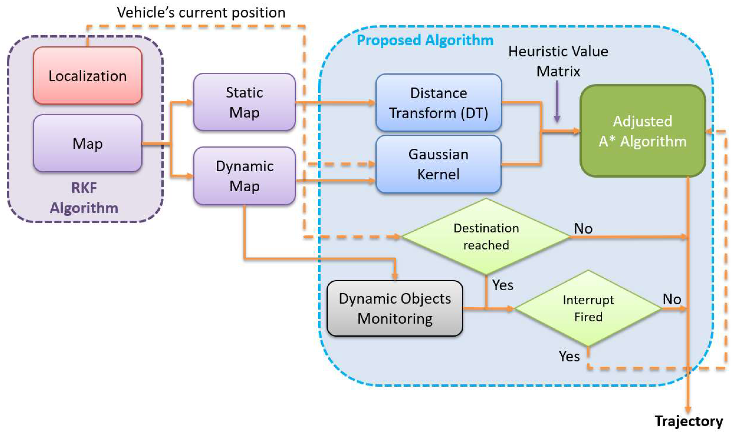
Section 2 illustrates an overview structure of the proposed method. The representation of the static and dynamic map objects is explained in
Section 3.
Section 4 demonstrates optimized real-time trajectory generation. Dynamic objects monitoring is illustrated in
Section 5. The experimental results are presented in
Section 6. Finally, the conclusion is provided in
Section 7.
6. Experimental Results
To evaluate the efficiency of the proposed path generation method, the proposed method is compared with A*, APF, RRT, and bidirectional RRT using simulated and real datasets in static and dynamic environments.
Table 1 shows the environment status and type for each experimental dataset. All the comparisons have been performed using the same computing platform (MATLAB) on a Dell Inspiron 7000 series, Intel core i7-7500U 2.7 GHz, 16 GB RAM, 64-bit operating system.
The adjusted A* algorithm generates a path within a square window, the dimension of the window is equal to the maximum detection range of the utilized laser scanner rangefinder, 6 m. Since the size of individual grid cell is 5 cm, and each grid cell represents a node. Therefore, the search domain is created from 240 × 240 nodes (i.e., grid cells).
For Dataset I,
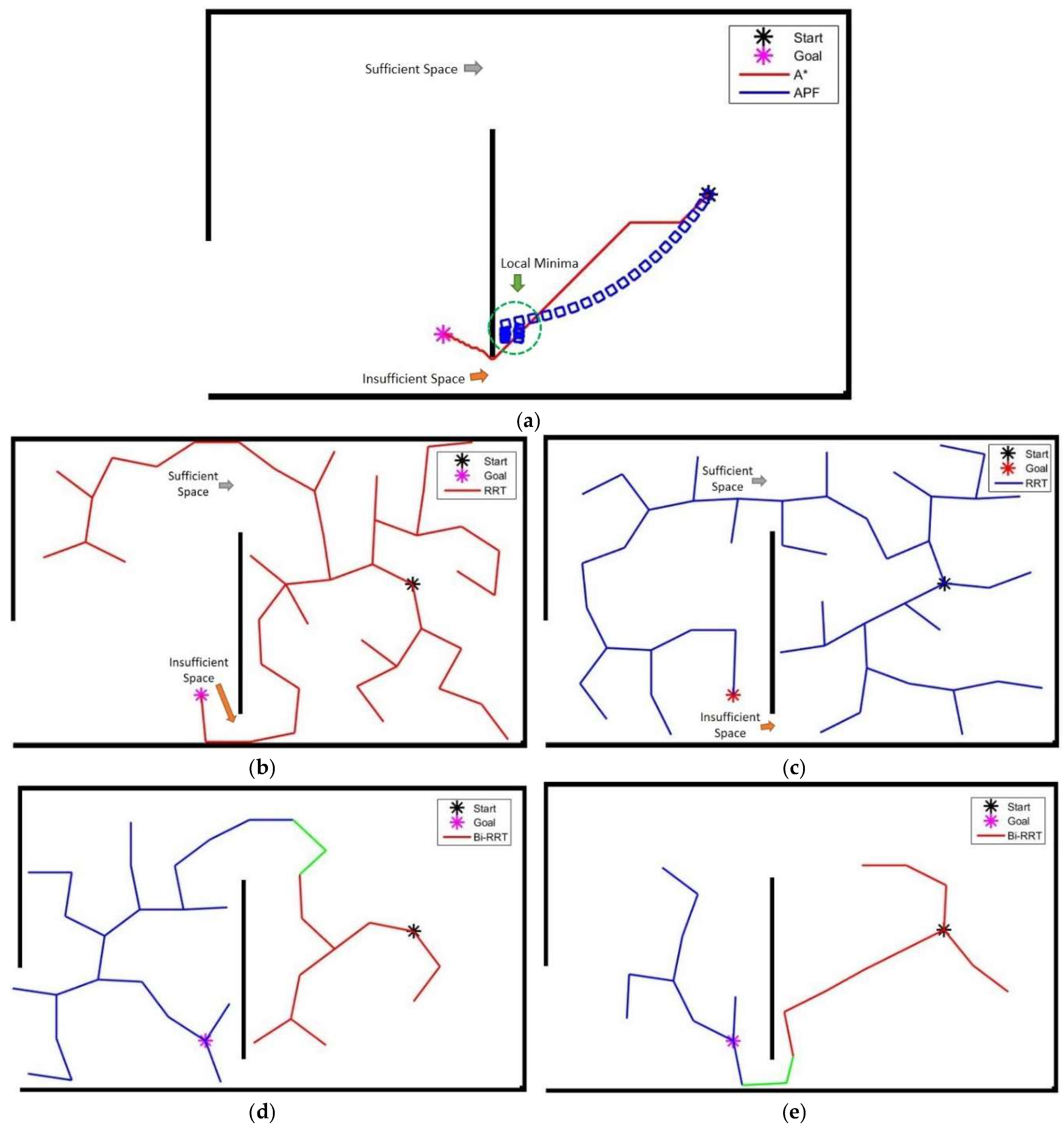
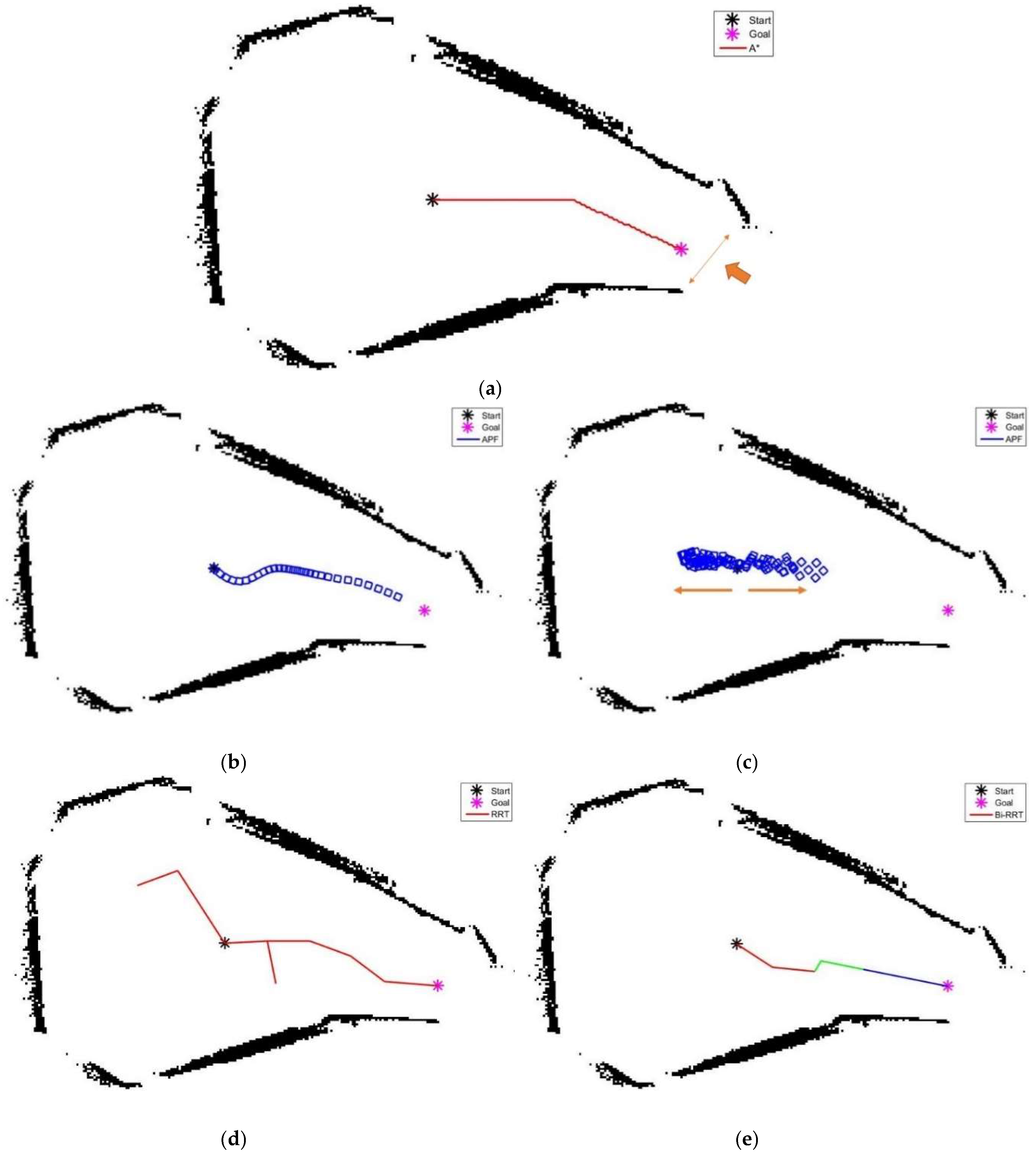
Figure 11 illustrates the simulation results of generating paths using A* algorithm, APF method, RRT algorithm and bidirectional RRT algorithm, respectively. The black and magenta asterisks represent the positions of the source and goal points, respectively. In
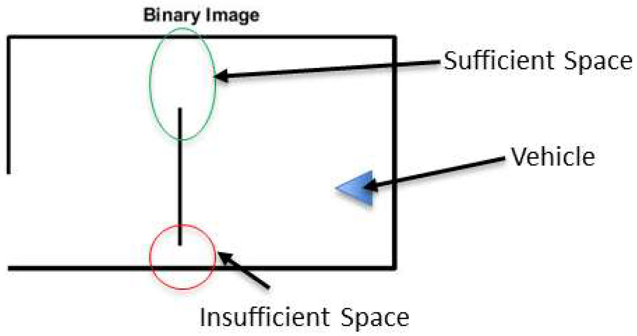
Figure 11a, the generated path using A* algorithm is represented by the red line, while the generated path using APF method is represented by the blue squares. The generated path of the A* algorithm passes through the insufficient space, as shown by the orange arrow, due to shortest path behavior of the algorithm. Furthermore, the generated path is chosen close to the static object, which exposes risk to the vehicle. The APF method fails to provide a solution because the method is trapped in local minima, as shown by the green circle. The processing time of the A* algorithm is 466 ms. The processing time of the APF method is not available because the method is trapped.
Figure 11b,c shows the generated paths using different iterations of RRT algorithm. The red and blue lines represent the generated paths in different iterations. It is clear that each iteration of the algorithm generates a new path due to the random nature of the algorithm. The generated path goes across the insufficient space, as shown in
Figure 11b, while the generated path goes across the sufficient space, as shown in
Figure 11c. Thus, the algorithm does not guarantee that the generated path passes through the sufficient space to reach the goal point. The processing times of the iterations are 3573 and 4205 ms.
Figure 11d,e demonstrates the generated paths using different iterations of bidirectional RRT algorithm. The red and blue lines represent the two generated trees from each seed (i.e., source and goal points). The green line represents the connection between the two trees. The algorithm also does not guarantee that the generated path passes through the sufficient space. The processing times of the iterations are 3312 and 2179 ms.
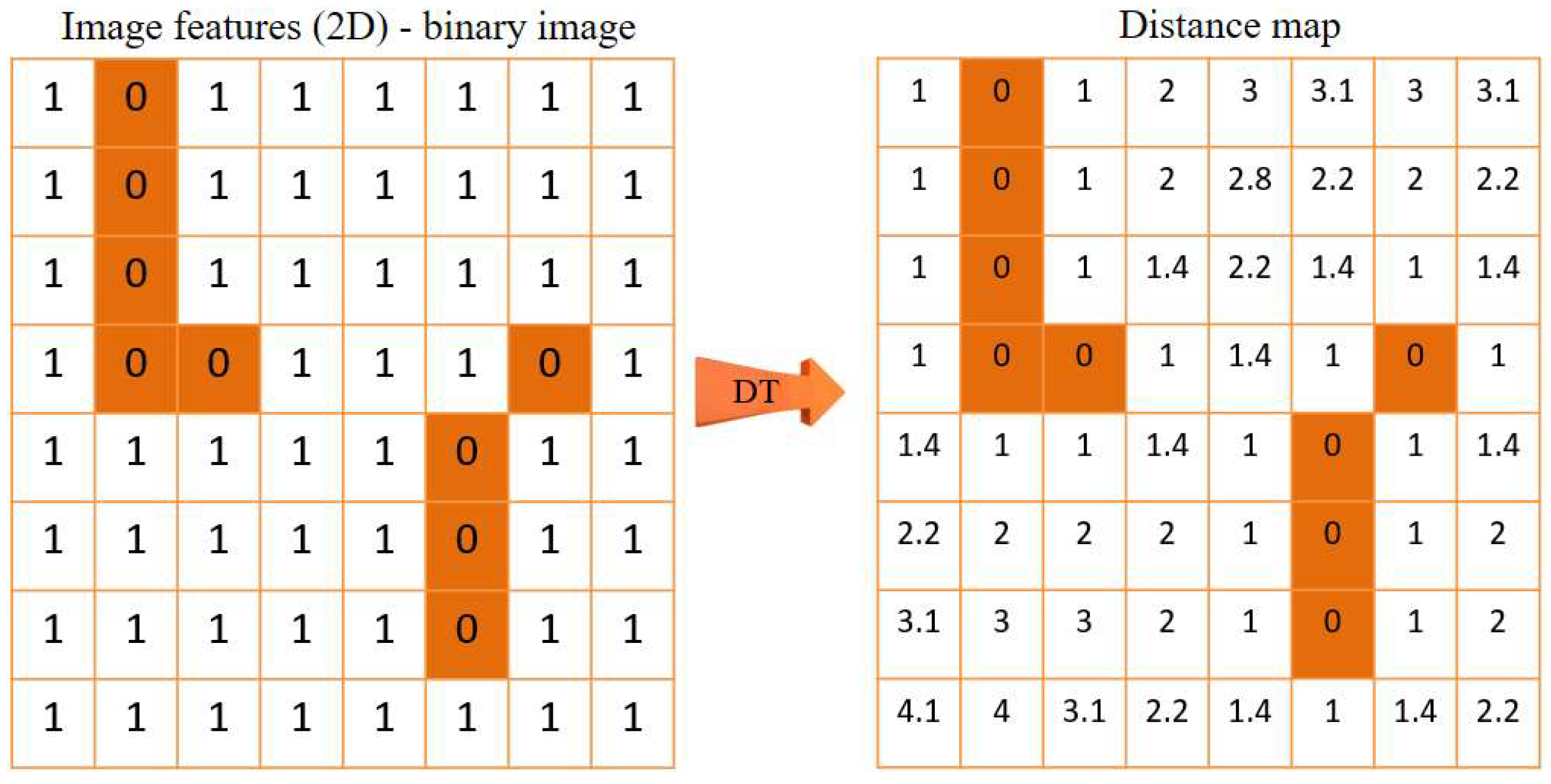
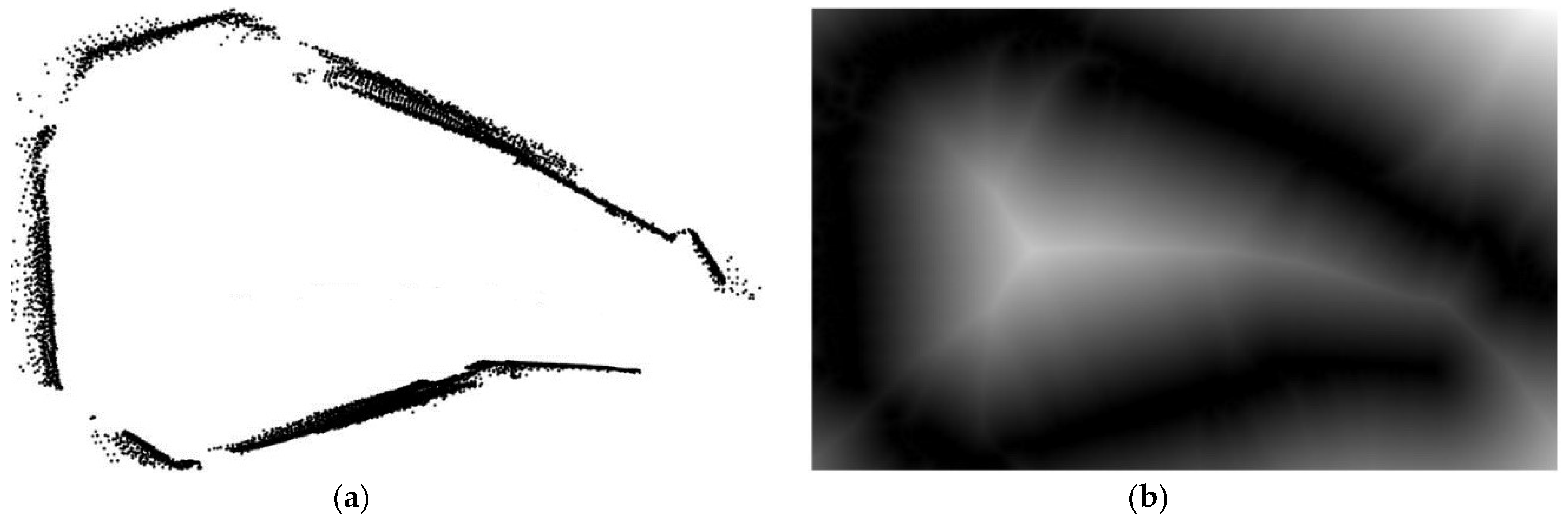
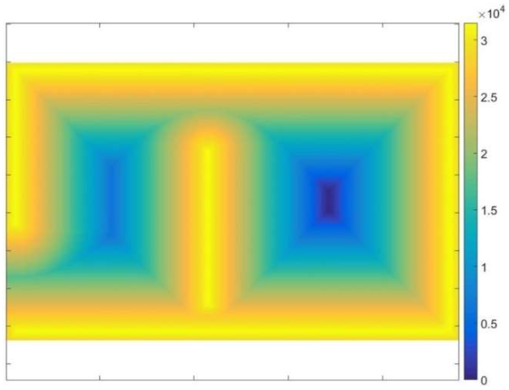
Figure 12 demonstrates the cost map of the static representation using the proposed method which is computed from the static objects only using the DT method. The static obstacles are represented by the brightest color which represents the highest cost, whereas the cost gradually decreases for the extension of the obstacles. On the other hand, the lowest cost is represented by the darkest color which represents the least available risky areas. This cost map is fed into the adjusted A* algorithm as a heuristic value.
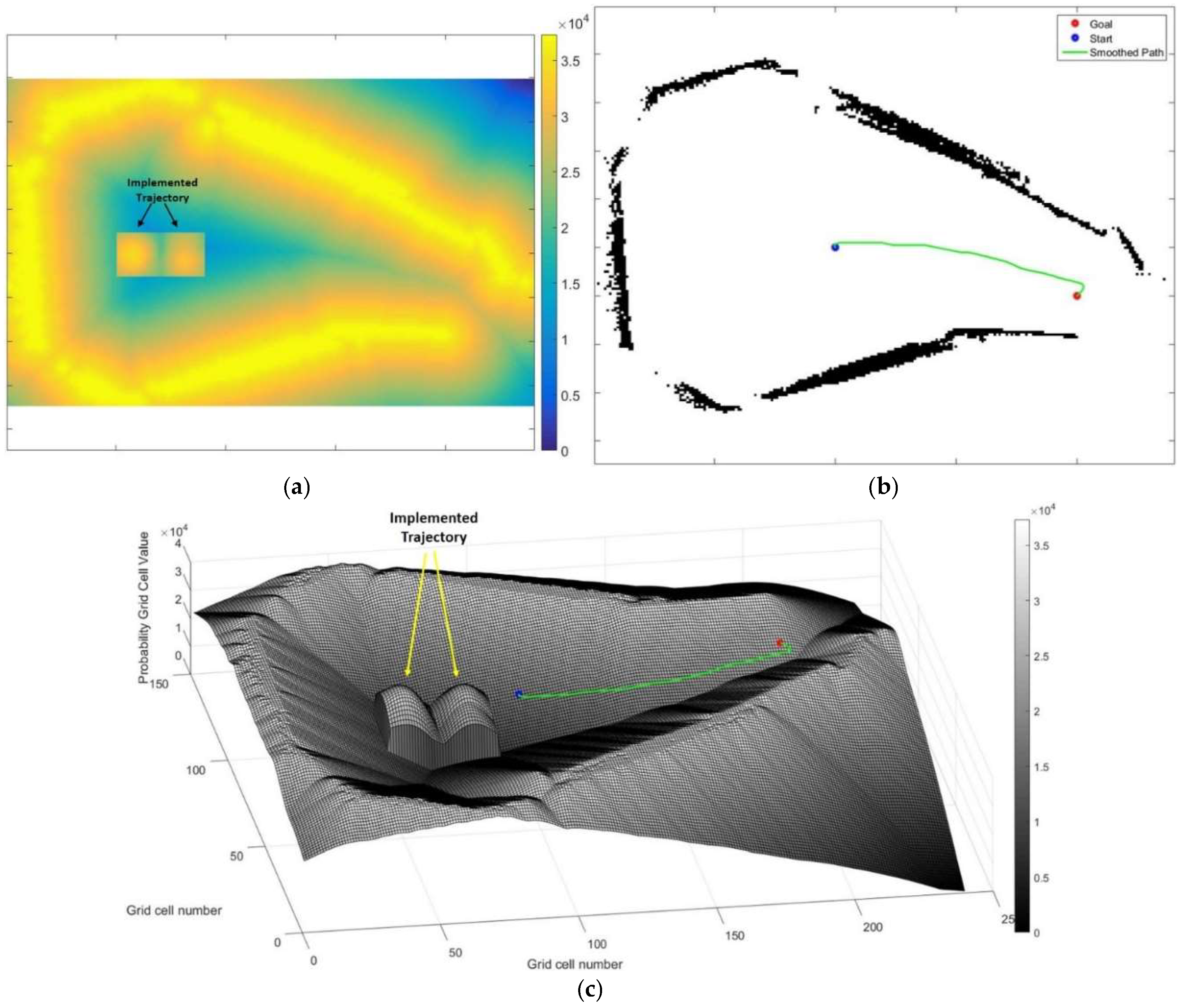
Figure 13 shows the generated trajectory within the extension of the static objects. The source point is represented by the blue asterisk, while the goal point is represented by the red asterisk. The generated path is represented by the green line. Obviously, the insufficient space is completely blocked by performing the obstacle extension process. Thus, the insufficient space will not be a candidate path for the vehicle. Moreover, the generated path adheres to the darkest color/least cost areas in the map to efficiently decrease the flight risk of the vehicle.
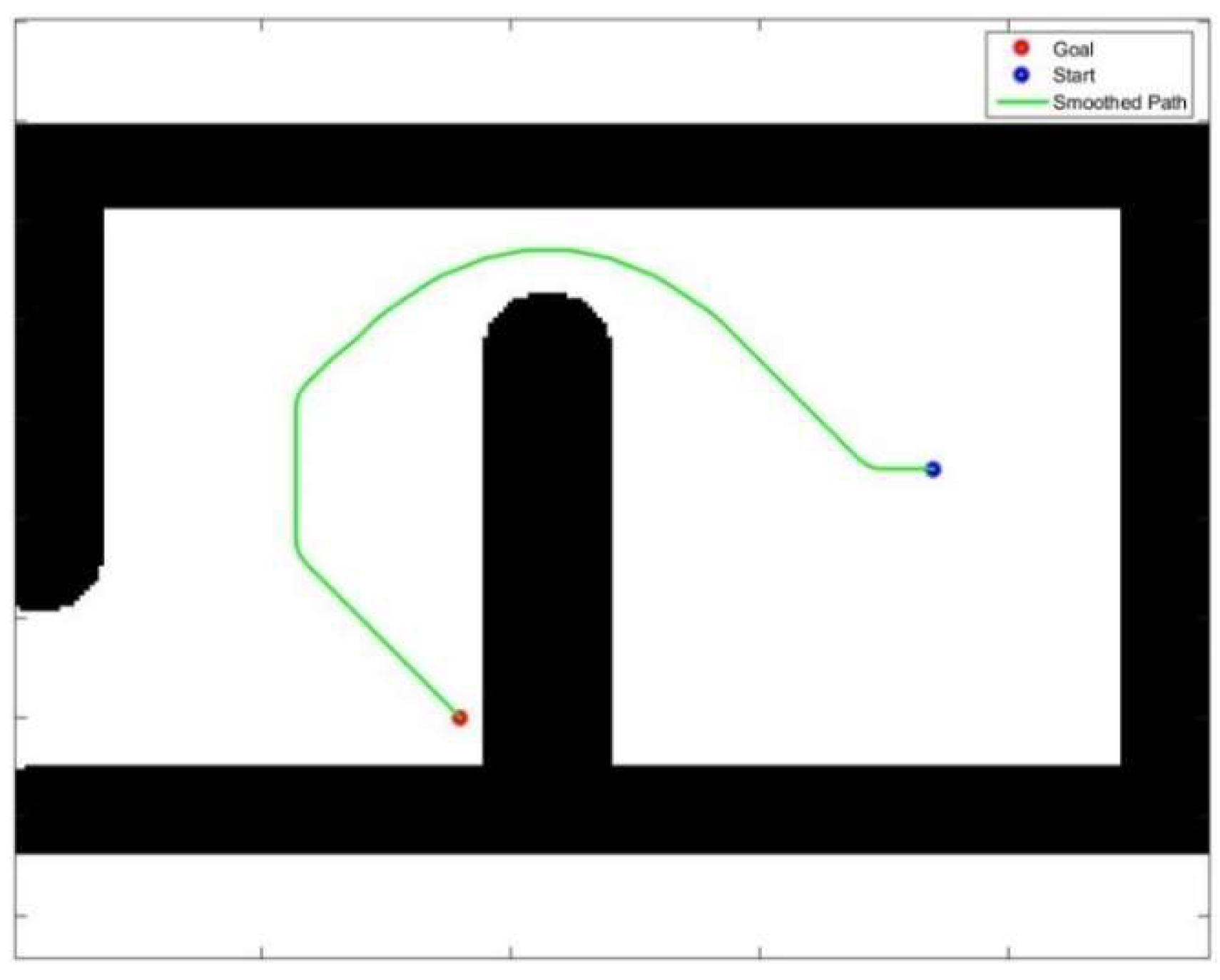
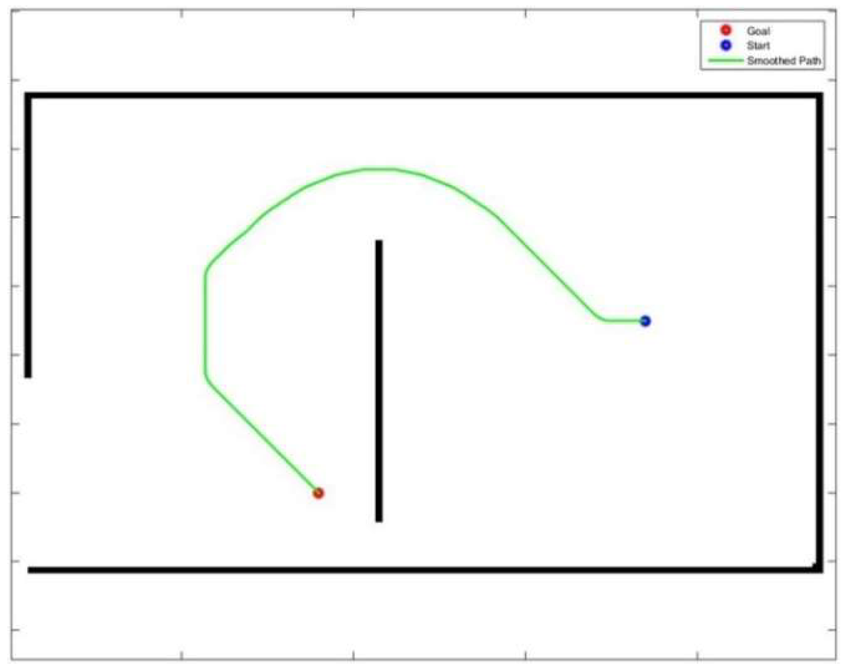
Figure 14 demonstrates the 2D representation of the generated path. The blue asterisk represents the position of the starting point, while the red asterisk represents the position of the goal point. The smoothed path is represented by the green line. Since the only factor affecting the path generation is the static environment, the generated path is attempted to be in the middle of the obstacles to minimize the risk of the generated path. The processing time of the proposed algorithm is 550 ms. The processing time has also been tested on a light weight board (UDOO X86) and the computed time is 610 ms. This embedded system consists of a single board computer which is based on Quad Core 64-bit new-generation X86 processors made by Intel
®®. This board meets the deployment requirements on small size UAVs [
29].
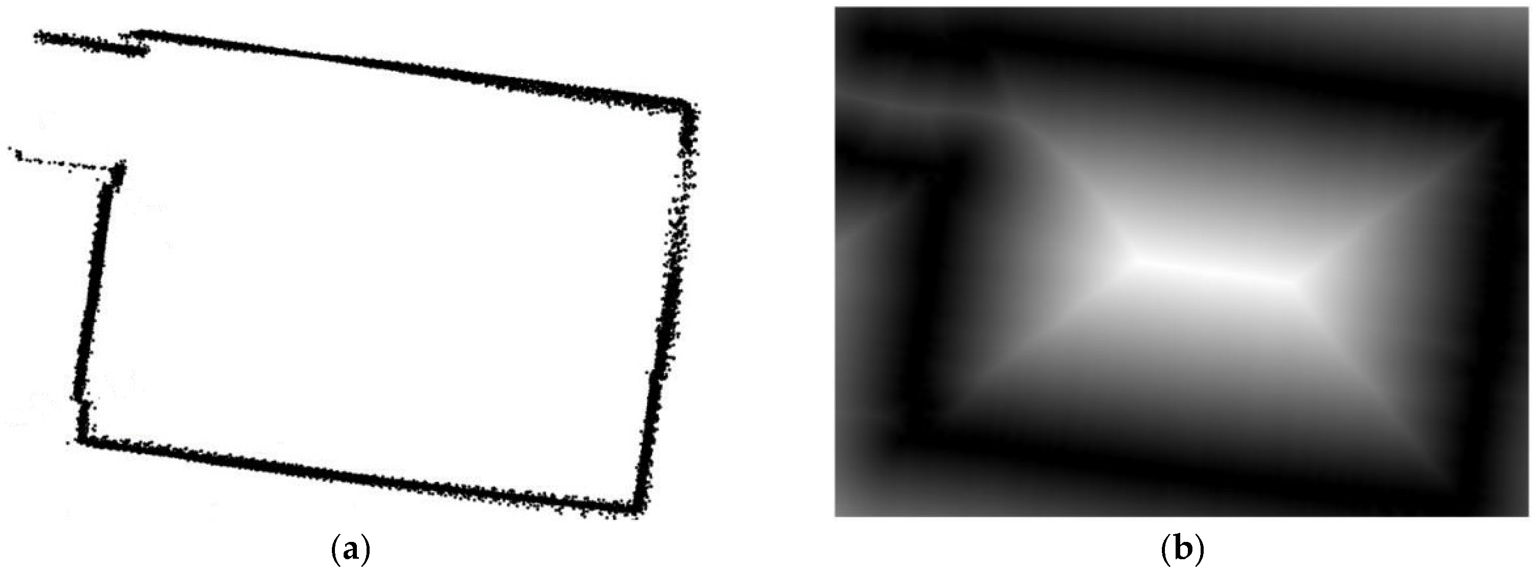
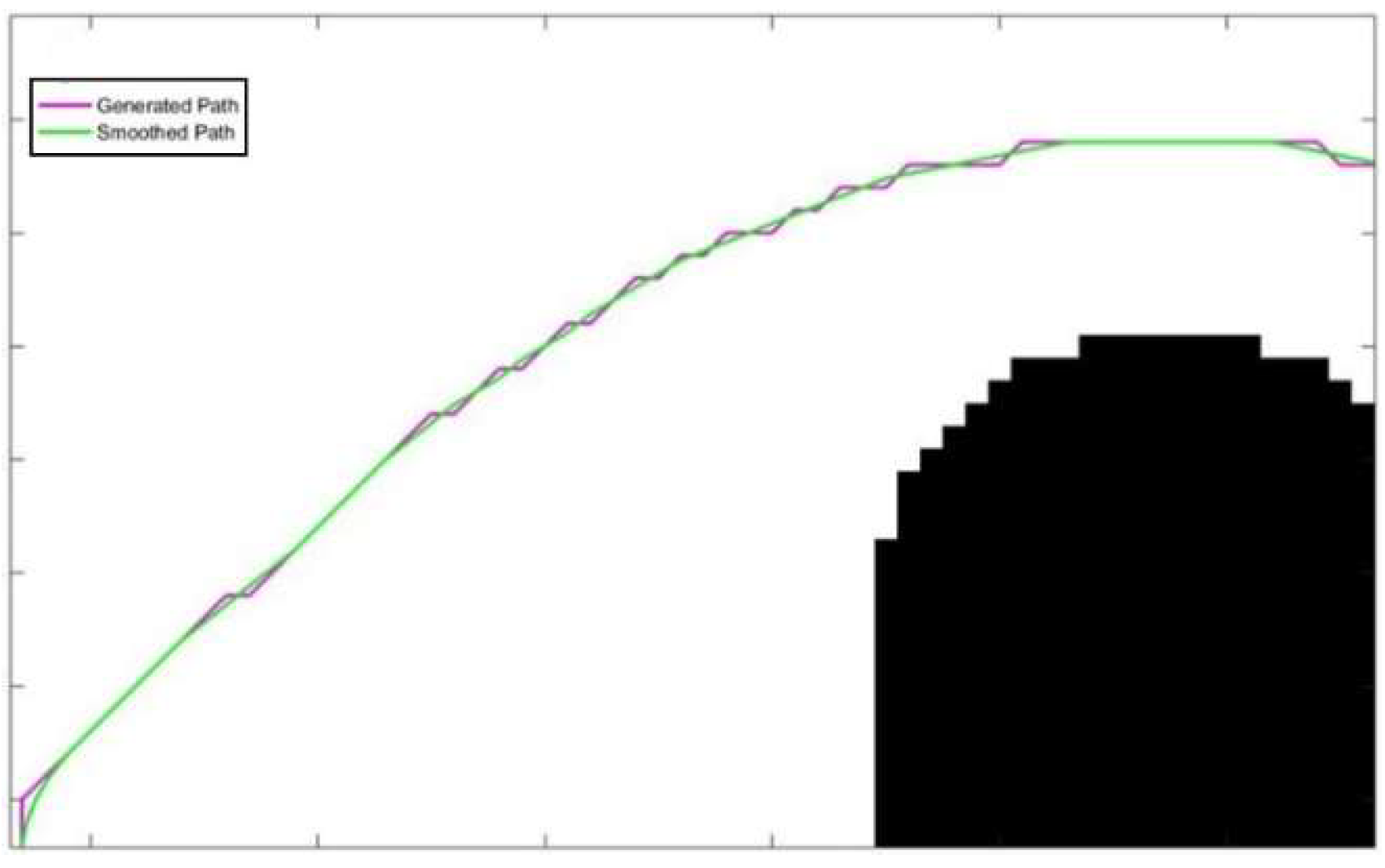
Figure 15 shows the generated path before and after smoothing process and it also represents a zoomed area of part of
Figure 14. The magenta line represents the generated path before the smoothing process. The green line represents the smoothing path. The generated path before the smoothing process is crimped. This behavior is because the constructed map is built using an occupancy grid. Subsequently, the generated path transfers from one cell to another without prejudice to the optimization goal (i.e., minimize the risk). The crimp behavior affects the smoothness of the flight which includes, but is not limited to, endurance time and battery consumption.
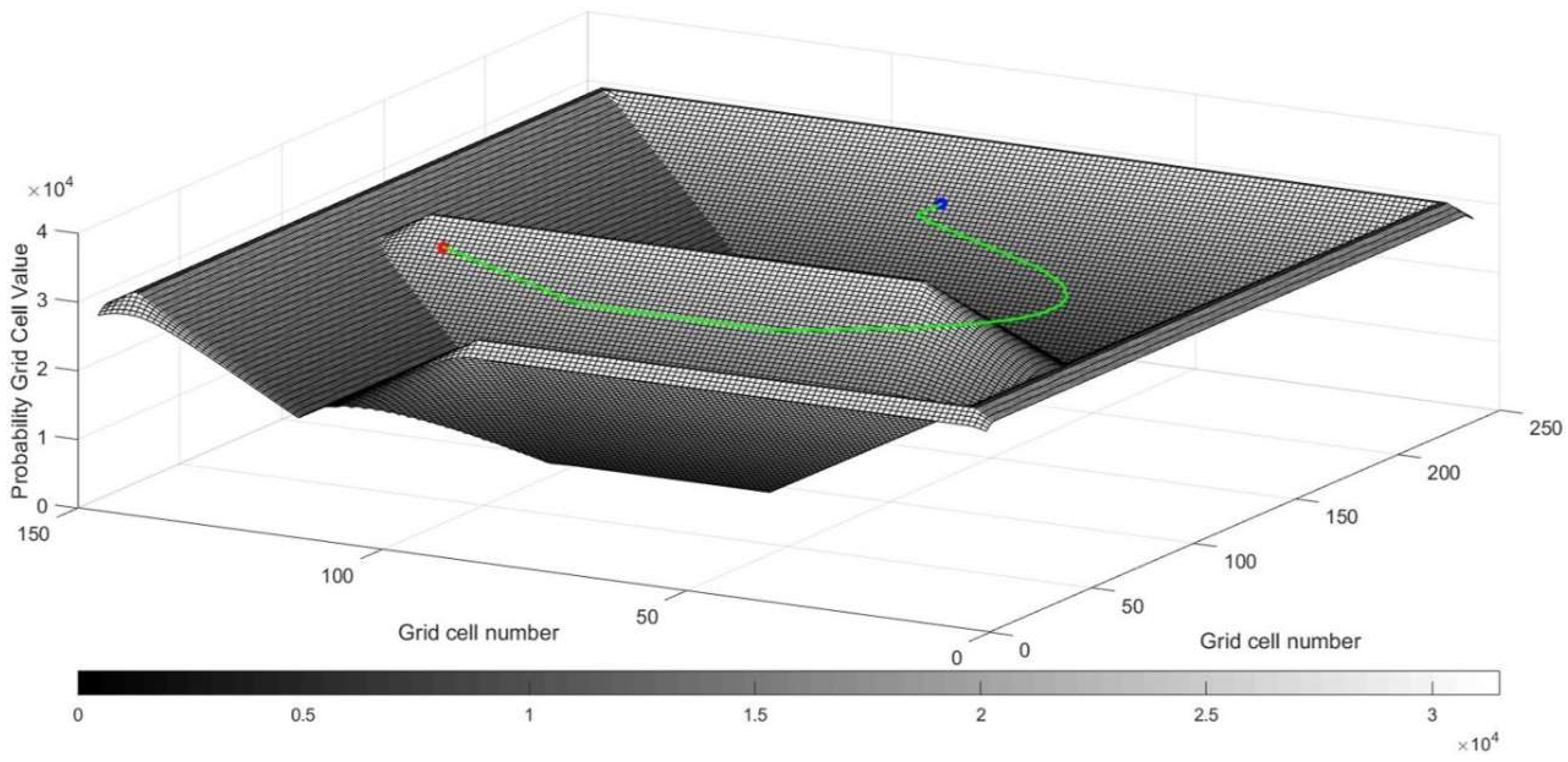
Figure 16 depicts the 3D representation of the generated path. The blue asterisk represents the starting position, while the red asterisk represents the goal position. The smoothed path is represented by the green line. As described above, the static obstacles are represented using the DT method. Thus, the maximum height is the maximum cost, and it represents the obstacle grid cells, which decreases in magnitude to represent the extension of the obstacles until reaches approximately the middle distance in-between the obstacles. It is clear that the generated trajectory is created inside the valley in-between the extended obstacles to prepare a safe path for the MAV.
For Dataset II,
Figure 17 illustrates the generated path using A* algorithm, APF method, RRT algorithm, and bidirectional RRT, respectively. The black and magenta asterisks represent the positions of the source and goal points, respectively. In
Figure 17a, the generated path is represented by the red line. The destination point is located between two close static objects as represented by the orange arrows. Since the current situation does not cause hurdles to the A* algorithm, an appropriate path is generated between the two close static obstacles. The processing time of the algorithm is 690 ms. Since the potential field is created depending on the attractive and the repulsive forces, the APF method is sensitive to their magnitudes. The current situation affects the result of the generated path according to the magnitudes of the attractive and repulsive forces. When the attractive force is much higher than the repulsive force, an appropriate path is generated, as shown in
Figure 17b. The processing time of the algorithm is 1826 ms. However, when the repulsive force is approximately equal to the attractive force, the APF method fails to generate a path, a back and forth behavior, as represented by the orange arrows, is observed. This is because, whenever the APF method tries to reach the trapped destination, between the two close obstacles, the repulsive forces of the two obstacles repel the generated path, as shown in
Figure 17c, which indicates the sensitivity of the APF algorithm to the successful tuning of the attraction and repulsion forces parameters.
Figure 17d,e shows the generated path using the RRT and bidirectional RRT algorithms, respectively. The generated path is represented by the red line as shown in
Figure 17d, while the red and blue lines are used to represent the generated path, as shown in
Figure 17e, and the green line is used as a conjunction between the bidirectional trees. Typically, the random behavior of both algorithms affects the result of the generated path, as it is changed every time the algorithm is conducted. The processing time of RRT and bidirectional RRT are 1229 and 854 ms, respectively.
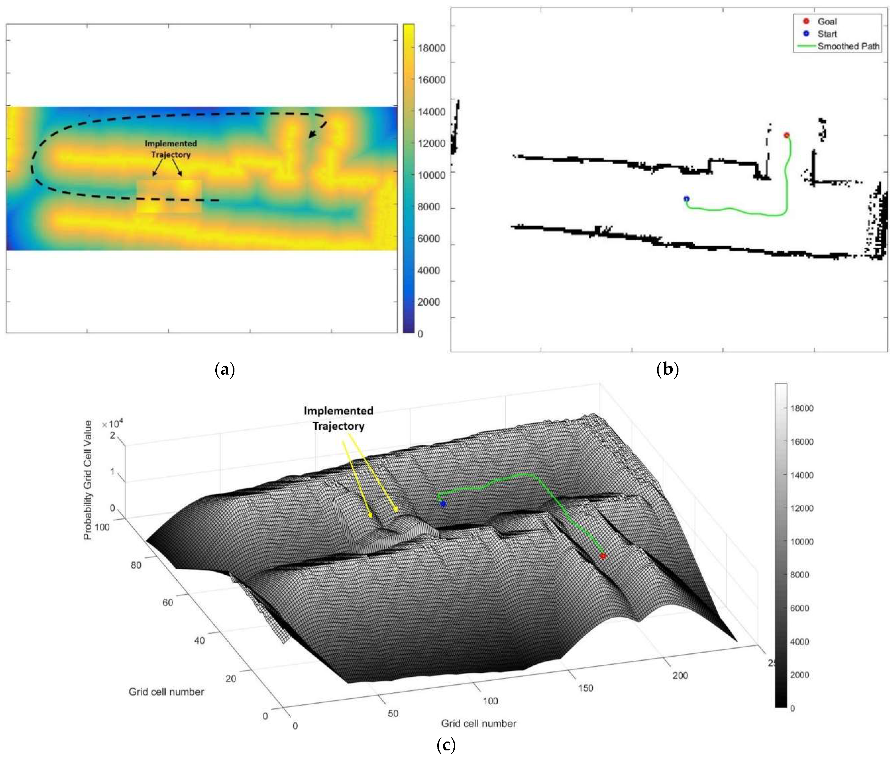
Figure 18 demonstrates the generated path using the proposed method in a static environment.
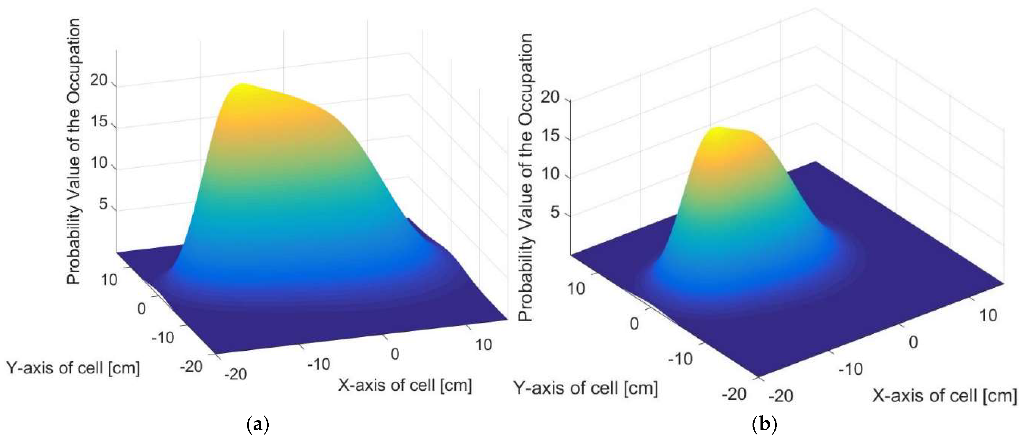
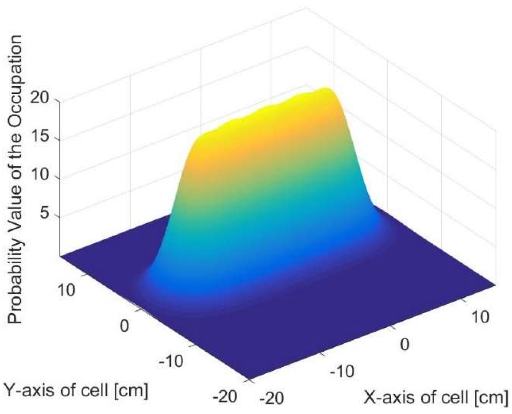
Figure 18a shows the cost map of the static representation. The brightest color represents the static obstacles (i.e., highest cost), whereas the cost gradually decreases for the extension of the obstacles. On the other hand, the darkest color represents the lowest cost which represents the least available risky areas. The previously executed trajectory is represented by the two bright squares as shown by the black arrows. The implemented trajectory is computed using the Gaussian kernel as mentioned earlier.
Figure 18b demonstrates the 2D representation of the generated path. The blue asterisk represents the starting position, while the red asterisk represents the goal position. The smoothed path is represented by the green line. Since the only factor affecting the path generation is the static environment, the generated path is attempted to be in the middle of the obstacles to minimize the risk of the generated path. The processing time of the algorithm is 399 ms.
Figure 18c depicts the 3D representation of the generated path. The blue asterisk represents the starting position, while the red asterisk represents the goal position. The smoothed path is represented by the green line. As described above, the static obstacles are represented using the DT method. Thus, the maximum height is the maximum cost, and it represents the obstacle grid cells, which decreases in magnitude to represent the extension of the obstacles until reaches approximately the area in-between the obstacles. It is clear that the generated trajectory is created inside the valley in-between the extended obstacles to prepare a safe path for the MAV. The protuberance, as indicated by the yellow arrows, represents the previously executed trajectory. These protuberances prevent the vehicle to revisit the same place twice to maximize the visited area.
Dataset III is characterized by the presence of dynamic objects that add more complexity to the environment.
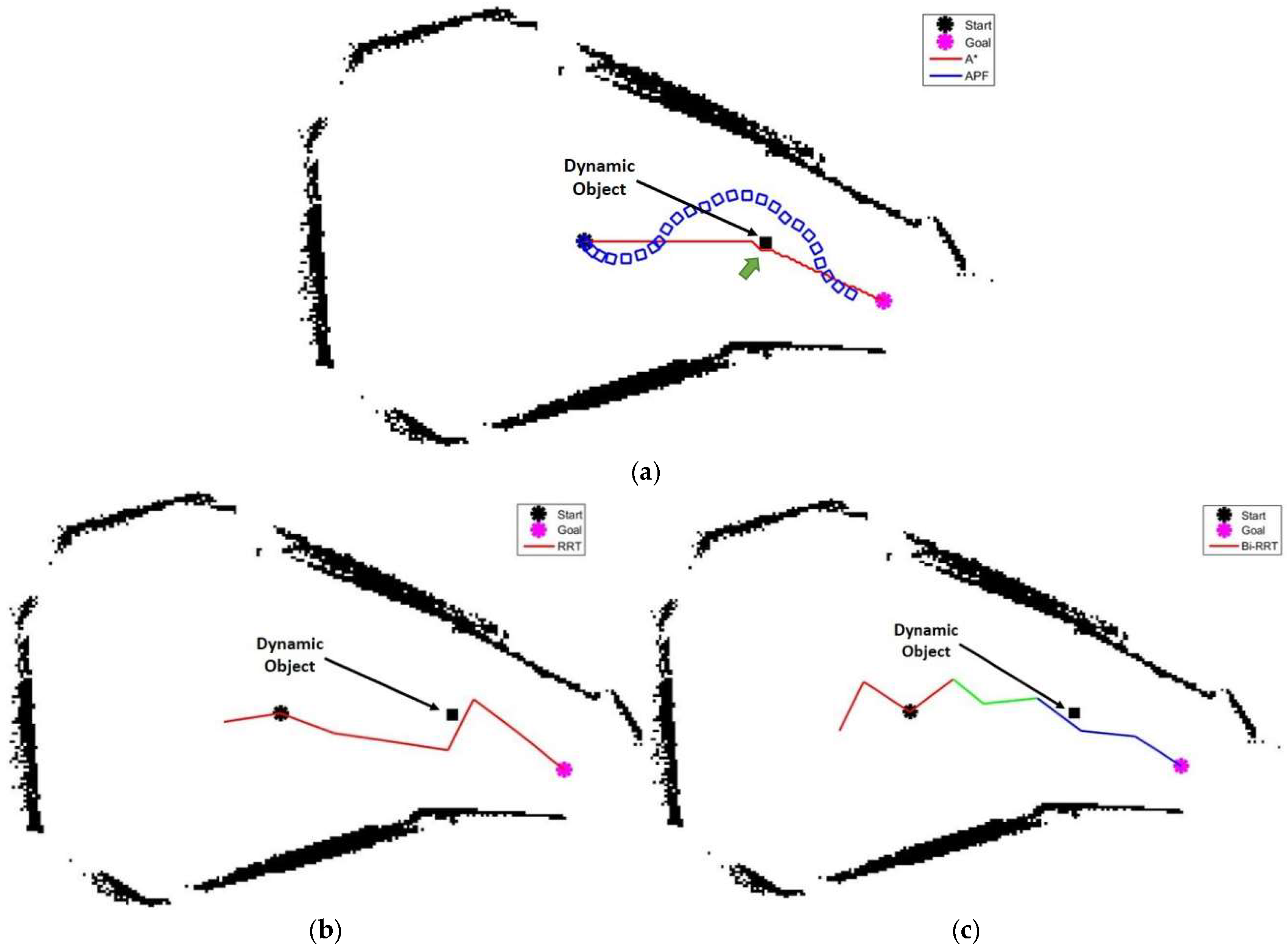
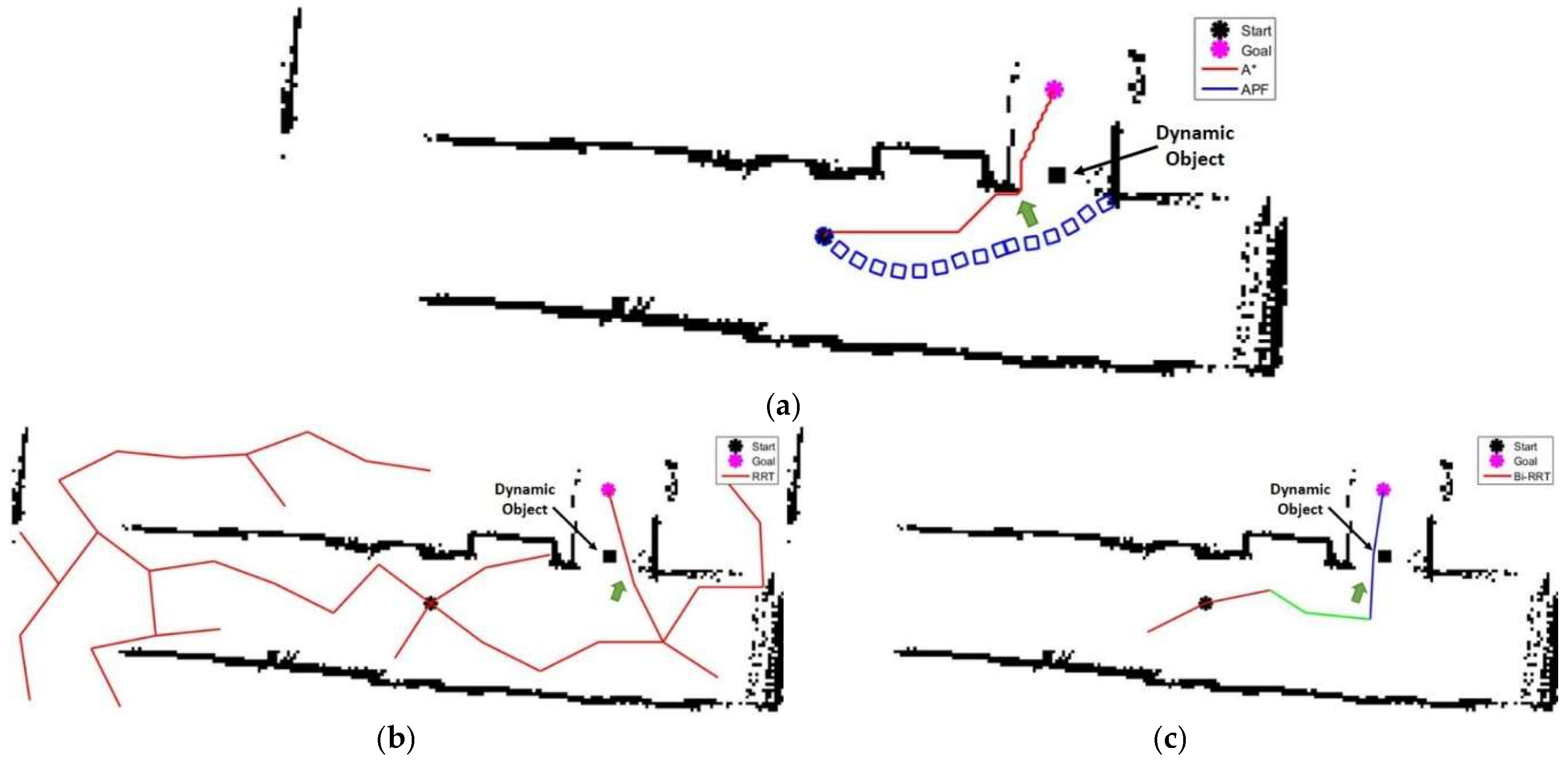
Figure 19 depicts the generated path using A* algorithm, APF method, RRT algorithm, and bidirectional RRT algorithm, respectively. The blue and magenta asterisks represent the positions of the source and goal points, respectively. The dynamic object is represented by the black square. In
Figure 19a, the generated path using A* algorithm is represented by the red line, while the generated path using APF method is represented by the blue squares. The A* algorithm deals with the dynamic object as a static object in the moment of generating the path. However, the algorithm cannot detect the movement of the dynamic object in the successive epochs unless the algorithm is re-run every epoch. Thus, extra computations have to be executed to achieve all the iterations. Even though the dynamic object stops at the time of generating the path, the shortest path behavior forces the generated path to be close to the dynamic object as shown by the green arrow. This obviously creates a risky situation for the vehicle. On the other hand, the APF method is influenced by the potential field that is produced from the attractive and repulsive forces from the goal and obstacles, respectively. Consequently, the potential field is frequently changing due to the effect of the moving object in the environment. Moreover, the APF method lacks the monitoring of the dynamic objects. Therefore, the traditional APF method fails to provide a solution in the dynamic environments [
19]. However, the trajectory is plotted as if the dynamic object stops at the time of generating the path. The processing time of the A* algorithm and the APF method are 684 and 2108 ms, respectively.
Figure 19b,c shows the generated path using the RRT and bidirectional RRT algorithms, respectively. The generated path is represented by the red line as shown in
Figure 19b, while the red and blue lines are used to represent the generated path, as shown in
Figure 19c, and the green line is used as conjunction between the bidirectional trees. The generated random path in the sample space at time (t) may be either occupied with a dynamic object soon (t + n), where n is a positive integer, or blocked by a dynamic object in the near future as well, as the dynamic object is changing its allocation every time. Consequently, a collision will occur between the vehicle and the dynamic object. The processing time of the RRT and bidirectional algorithms are 1085 and 935 ms, respectively.
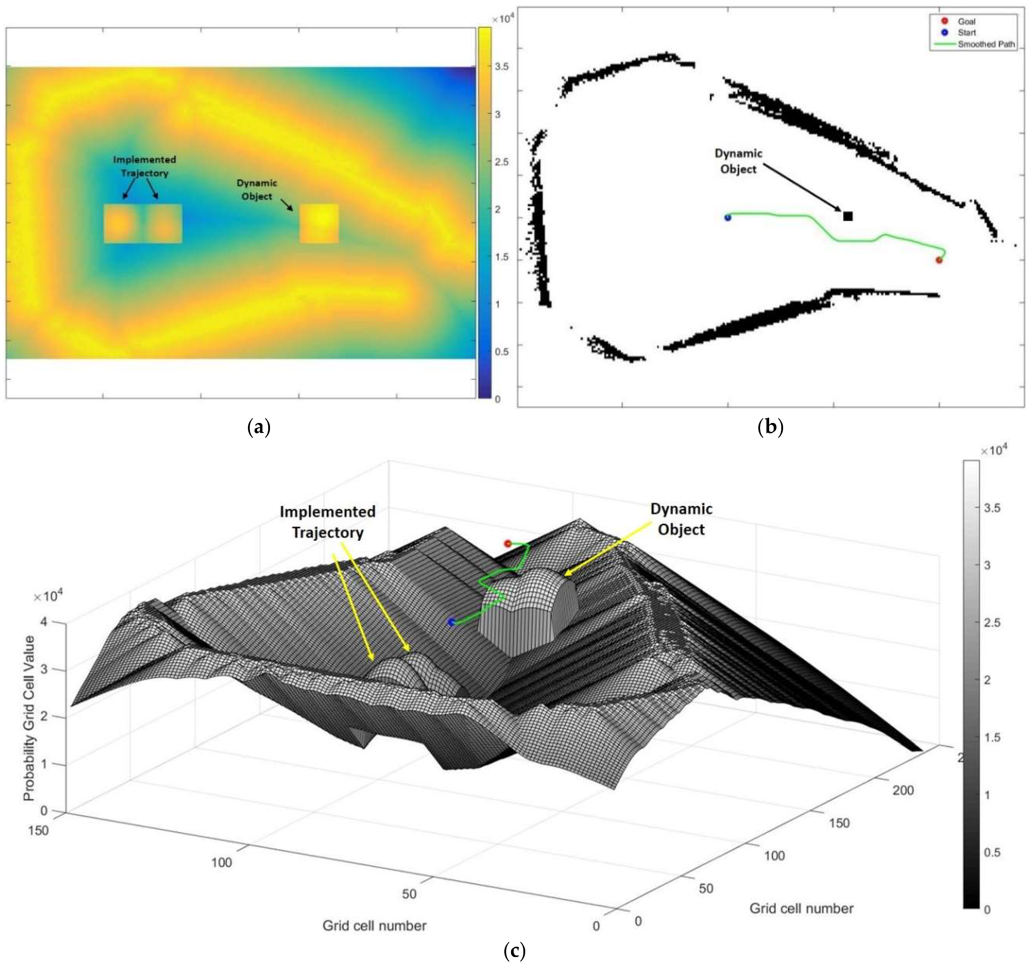
Figure 20 demonstrates the generated path using the proposed method in a dynamic environment.
Figure 20a shows the cost map of the static and dynamic representations, which is computed from the static and dynamic objects using the distance transform method and Gaussian kernel, respectively. The brightest color represents the highest cost which is the static, implemented trajectory and dynamic object. The previously executed trajectory is represented by the two successive bright squares. The previously executed trajectory is represented using the Gaussian kernel. The dynamic object is represented by the bright square which is computed using the Gaussian kernel as well. On the other hand, the darkest color represents the lowest cost which represents the least available risky areas. This cost map is fed into the adjusted A* algorithm as a heuristic matrix.
Figure 20 demonstrates the 2D representation of the generated path. The blue asterisk represents the starting position, while the red asterisk represents the goal position. The smoothed path is represented by the green line. The black square represents a dynamic object. By comparing the static and dynamic results of the proposed method, it is clear that the generated path deviates to avoid the dynamic object and minimize the risk of the generated path. The amount of the deviation varies according to the static and dynamic costs. For crowded environments, the cost of the dynamic objects is approximately high with respect to the static cost, but for uncongested environments, the cost of the dynamic objects is approximately low with respect to the static cost. The processing time of the algorithm is 374 ms.
Figure 20c demonstrates the 3D representation of the generated path. The blue asterisk represents the starting position, while the red asterisk represents the goal position. The smoothed path is represented by the green line. The consecutive protuberances represent the previously executed trajectory, while the single protuberance represents the dynamic object. The performed deviation depends on the total computed costs from the static and dynamic objects in the current scene. It is clear that the generated path endeavors to avoid the dynamic object and simultaneously avoids proximity to the static object according to their costs.
For Dataset IV,
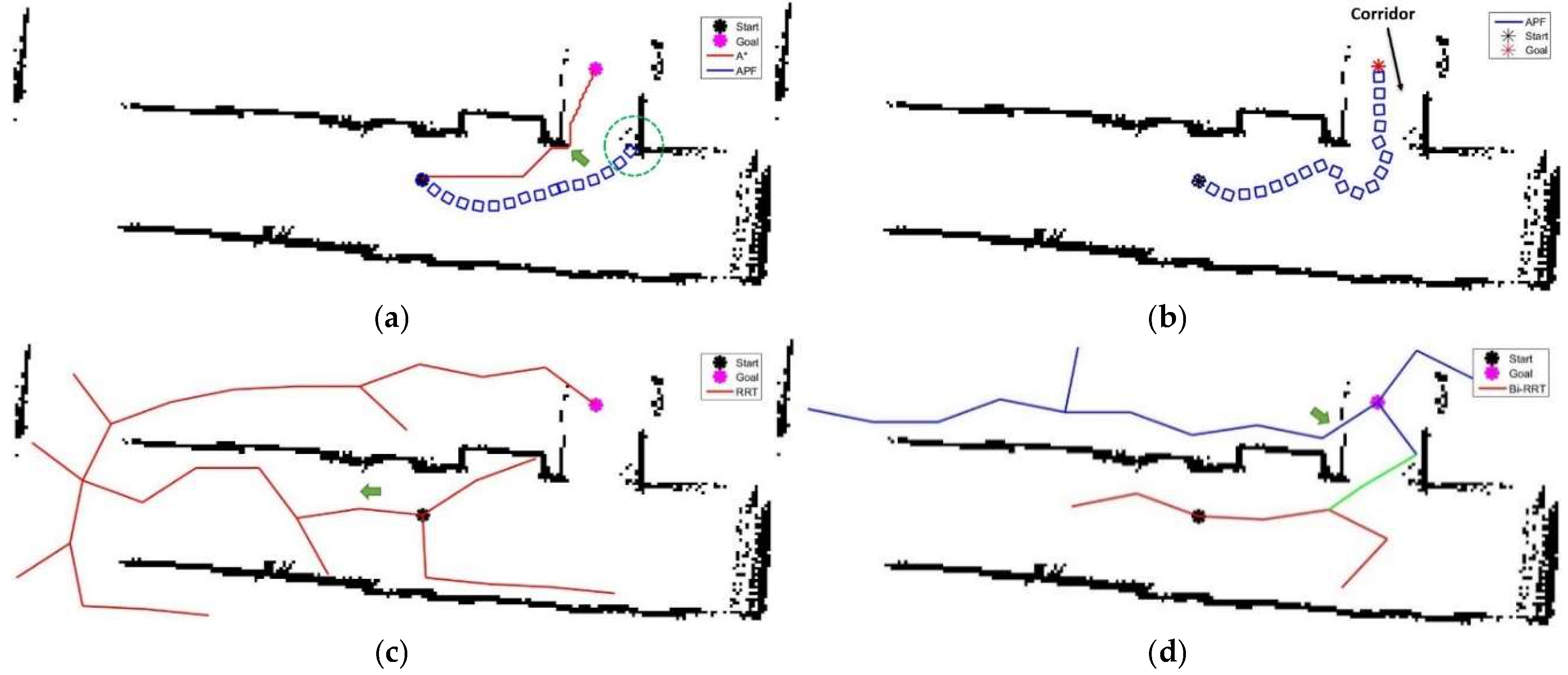
Figure 21 illustrates the generated paths using A* algorithm, APF method, RRT algorithm, and bidirectional RRT algorithm. The black and magenta asterisks represent the positions of the source and goal points, respectively. In
Figure 21a, the generated path using A* algorithm is represented by the red line, while the generated path using APF method is represented by the blue squares. The generated path of the A* algorithm is not far from the static obstacle, as shown by the green arrow, due to shortest path behavior of the algorithm. This closeness increases the risk of the vehicle. Due to the attraction and repulsion forces of the goal and obstacles, respectively, as well as the dynamic of the vehicle, the generated path of the APF method fails to reach the goal as the vehicle collides with the static object, as shown by the green circle. The processing time of the A* algorithm is 131 ms, while the processing time of the APF method is not available due to the collision.
Figure 21b shows the generated path of different iteration using APF method. The source and goal points are represented by the black and red asterisks, respectively. The generated path is plotted by the blue squares. Since the APF method is sensitive to the attraction and repulsion forces, as well as the corridor width, which is approximately 120 cm. The attractive force is tuned to be much greater than the repulsion force. As a result, a generated path is created from the source point to the goal point. The processing time is 2172 ms.
Figure 21c,d shows the generated path using the RRT and bidirectional RRT algorithms, respectively. The generated path is represented by the red line, as shown in
Figure 21c, while the red and blue lines are used to represent the generated path, as shown in
Figure 21d, and the green line is used as a conjunction between the bidirectional trees. In addition to the diversity of the results in each iteration due to the random behavior of both algorithms, both algorithms can build new intermediate nodes far away from the goal point that consumes time. The RRT algorithm generates the path in the opposite direction of the movement, as shown by the green arrow. Thus, the RRT algorithm can revisit the same place twice. The bidirectional RRT creates intermediate nodes through small gaps due to the miss occupation in the static obstacles, as presented by the green arrow. The processing times of the RRT and bidirectional RRT are 2839 and 1320 ms, respectively.
Figure 22 demonstrates the generated path using the proposed method in a static environment.
Figure 22a shows the cost map of the static representation. The brightest color represents the static obstacles (i.e., highest cost), whereas the cost gradually decreases for the extension of the obstacles. On the other hand, the darkest color represents the lowest cost which represents the least available risky areas. The previously executed trajectory is represented by the two bright squares, as shown by the black arrows. Due to the presence of the high cost of the previously executed trajectory, the MAV cannot go back to reach the goal point, as shown by the dashed arrow, to maximize the visited area.
Figure 22b demonstrates the 2D representation of the generated path. The blue asterisk represents the starting position, while the red asterisk represents the goal position. The smoothed path is represented by the green line. Obviously, the generated path is attempted to be in the middle of the obstacles as usual under different scenarios to minimize the risk of the generated path. The processing time of the algorithm is 286 ms.
Figure 22c depicts the 3D representation of the generated path. The blue circle represents the starting position, while the red circle represents the goal position. The smoothed path is represented by the green line. As described above, the implemented trajectory is represented using the Gaussian kernels. Thus, the protuberance represents the occurrence of the implemented trajectory as shown by the yellow arrows. Thus, the vehicle is driven to explore new places to maximize the visited area.
For Dataset V, a dynamic scenario is created in which a dynamic object moves inside a narrow corridor where the MAV cannot safely pass.
Figure 23 depicts the generated path using A* algorithm, APF method, RRT algorithm, and bidirectional RRT algorithm. The black and magenta asterisks represent the positions of the source and goal points, respectively. In
Figure 23a, the generated path using A* algorithm is represented by the red line, while the generated path using APF method is represented by the blue squares. Despite the existence of a dynamic object in the entrance of the corridor, the A* algorithm generates a path through the corridor to reach the goal point. Furthermore, the generated path is near to the static object, as shown by the green arrow. This obviously creates a risky situation for the vehicle. On the other hand, the APF method fails to reach the goal point, and a collision occurs due to the repulsive forces that are generated from the static and dynamic objects. The processing time of the A* algorithm is 136 ms, while the processing time of the APF method is not available due to the collision.
Figure 23b shows the generated path using the RRT algorithm. The generated path is represented by the red line. The generated path is also passed across the corridor beside the dynamic object, as shown by the green arrow, to reach the goal point. This also creates a risky situation for the MAV. The processing time of the RRT algorithm is 2323 ms.
Figure 23c shows the generated path using the bidirectional RRT algorithm. The red and blue lines are used to represent the generated path and the green line is used as a conjunction between the bidirectional trees. The algorithm generates the path through the corridor and closes to the dynamic object. The vehicle is exposed to the same risky situation. The processing time of the bidirectional RRT algorithm is 436 ms.
On the other hand, the proposed method does not generate a path to the destination, due to the movement of the dynamic object in the entrance of the corridor, to minimize the risk on the vehicle. Hence, the proposed method either keeps the vehicle for a certain period until the dynamic object moves or generates a new path to a new destination if feasible. Ultimately,
Table 2 illustrates a comparison between the proposed method among other methods/algorithms. It is clear that the proposed method generates a path and safely reaches the goal in all the experiments except the last experiment as aforementioned. Furthermore, the proposed method is characterized by the largest average distance to the nearest obstacle with the least average processing time.
7. Conclusions
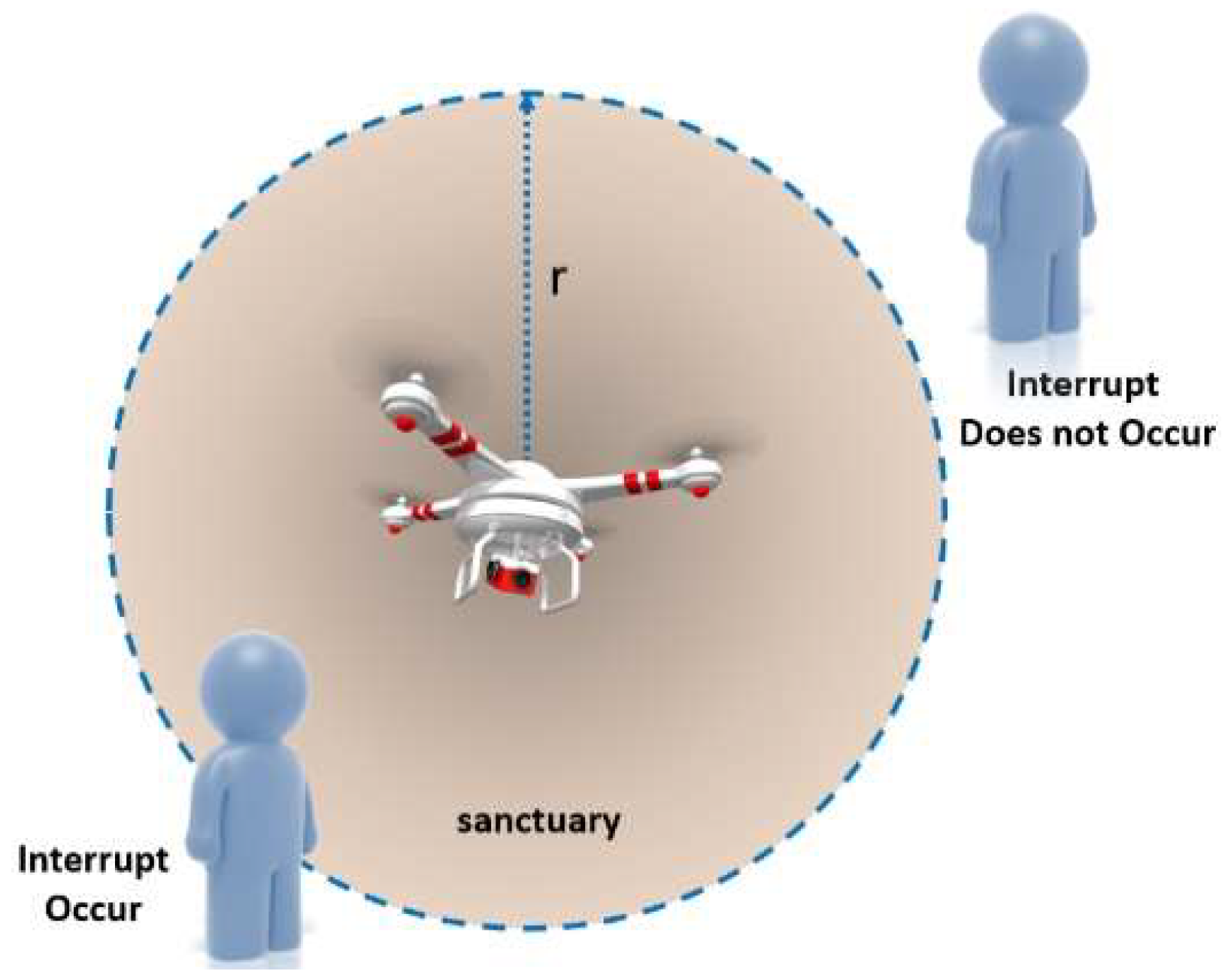
In robotics, path planning is a problem of finding a proper trajectory from the current position to a definite destination, according to the limitations of the environment and the vehicle. The environment could be unknown and/or dynamic, while the limitations of the vehicle can be for instance the vehicle’s size and maximum velocity of the vehicle. The objective of path planning problem varies based on the application requirements such as finding the shortest path or the fastest path. The time constraint is a critical factor in most path planning problems, especially search and rescue operations. Hence, maximizing the visited area during such operations is a fundamental task. Furthermore, minimizing the risk on the generated path is also an important task. Therefore, an efficient exploration method is proposed to maximize the visited area of unknown static/dynamic environment and simultaneously minimize the risk of the generated path. The proposed method builds the cost function of the static objects using the distance transform method, while uses the Gaussian kernel for the representation of the dynamic objects. Furthermore, the previously executed trajectory is represented by Gaussian kernels as a cost function. Thus, the proposed method generates the path that achieves the minimum summation of the cost functions. Additionally, the proposed method can reevaluate the destination and the trajectory for sudden situations because an interruption is fired once an interception of a dynamic object occurs inside the sanctuary area around the vehicle. Ultimately, the previously executed trajectory is recorded for the entire mission, and the proposed method uses this trajectory during the exit process for time saving. For validation and evaluation, the efficiency of the proposed method is compared with various algorithms and methods, such as A* algorithm, APF method, RRT algorithm, and bidirectional RRT, under different scenarios. The proposed method exhibits efficiency in avoiding both static and dynamic obstacles. The average distance to the nearest obstacle of the A* algorithm, APF, RRT, bidirectional RRT, and the proposed method is 12, 53, 44.3, 45.4, and 64 cm, respectively. The proposed method maximizes the visited area as it never goes to same place twice. Furthermore, the average processing time of the A* algorithm, APF, RRT, bidirectional RRT, and the proposed method is 421.4, 2035.3, 2542.3, 1506.0, and 402.2 ms, respectively. The proposed results indicate the eligibility of the proposed method for real-time applications.


