Mapping the Changes in Urban Greenness Based on Localized Spatial Association Analysis under Temporal Context Using MODIS Data

Abstract

Vegetation plays an irreplaceable role for urban ecosystem services. Urban greenness represents all vegetation cover in and around cities. Understanding spatiotemporal patterns of the changes in urban greenness (CUG) provides fundamental clues for urban planning. The impact on CUG can be roughly categorized as being climate-induced and human-induced. Methods for mapping human-induced CUG (H-CUG) are rare. In this paper, a new framework, known as Localized Spatial Association Analysis under Temporal Context (LSAA-TC), was proposed to explore H-CUG. Localized spatial association analysis (LSAA) was performed first to extract local spatial outliers (LSOs), or locations that differ significantly in urban greenness from those located in the neighborhood. LSOs were then analyzed under the temporal context to map their intertemporal variations known as spatiotemporal outliers. We applied LSAA-TC to mapping H-CUG in the Wuhan Metropolitan Area, China during 2000–2015 using the vegetation index from Moderate-resolution Imaging Spectroradiometer (MODIS) 13Q1 as the proxy for urban greenness. The computed H-CUG demonstrated apparent spatiotemporal patterns. The result is consistent with the fact that the traditional downtown area presents the lowest H-CUG, while it is found that the peripheral area in the circular belt within 14–20 km from the urban center demonstrates the most significant H-CUG. We conclude that LSAA-TC can be a widely applicable framework to understand H-CUG patterns and is a promising tool for informative urban planning.

1. Introduction

Urbanization is undergoing rapid increases across the world, especially in some developing countries like China [1,2]. Although urbanized areas cover only a small portion of the earth’s surface, they provide more advantageous conditions through better education, convenient healthcare, more job opportunities, and improved urban infrastructure than rural areas [3,4]. Urbanization is typically associated with an improved living infrastructure, such as convenient transportation networks and more commercial centers, as well as a synchronized process of spatial growth and scattering of built-up areas that used to be for agricultural purposes [5,6]. As a result, the positive result from urbanization enables more inhabitants to enjoy the convenient life through living in cities. At the same time, urbanization has also incurred many significant negative changes, resulting in degraded urban ecosystem services in some aspects, such as loss of vegetated land, and has created heat islands, traffic jams, and air pollution [7,8]. Particularly, the continuously shrinking green vegetation space in urban and suburban areas has been a critical issue for sustainable urban development and public health in many cities [7]. It was reported that nine out of thirteen cities in England had exhibited declined extent in urban vegetation cover during 2000–2008 [9]. Significant vegetation losses were also observed in some big cities, such as Shanghai and Tianjin in China, over the last few decades [10]. The changes in urban vegetation space, typically associated with urban expansion, critically need to be investigated to provide their inhabitants with more sustainable urban ecosystem services [8,11,12].

Vegetation supports sustainable urban development [7,13]. As the principal component in the garden city concept (GCC), vegetation was found to have a consistent cooling effect on the canopy layer temperature in some tropical cities [14]. Due to the migration of population from remote rural areas to cities, the impact of human activities on urban land use is expected to intensify [9,15]. The human activities, as well as the uncontrolled land exploitation, have been recognized as the main threat for the vulnerability of urban ecosystem services [16]. Urban population growth not only accounts for urban sprawl but also leads to the degradation of vegetation [15,16]. The close relationship between human activities, land cover changes, and the ecosystem services in urbanized areas has been confirmed previously [17]. The vegetated areas (e.g., farmland, forest, or grassland) are often targeted as the frontier for land exploitation in the process of urban expansion. Due to this fact, the spatiotemporal changes in urban greenness can, to some extent, indicate urban land cover changes and possibly the level of interactions between land cover and human activities [18]. Urban greenness is an overall representation of all vegetation covers within and around cities, e.g., street plantation, lawns, parks, gardens, crops, wetlands, grasslands, and forests [19]. Those vegetation elements are listed as the “ecological infrastructure” for delivering ecosystem services in urbanized areas. Exploring the spatiotemporal patterns in the variations of urban greenness can shed some important insights on the changes of urban ecosystem services.

A number of approaches are proposed to map vegetation space in urban areas [13,20,21,22]. An on-site survey serves as the traditional means of measuring and monitoring vegetation distribution and abundance, but it is time-consuming and labor-intensive. Instead, remote sensing technology now seems to have become the dominant way, considering its cost-effectiveness and high efficiency [20,23]. Remotely sensed imagery acquired by various platforms (ground-based, airborne, or satellite) has been extensively applied in vegetation mapping [24]. The greenness density, indicated by vegetation indices (VIs), can be inversed from remote sensing images to quantify vegetation abundance [25,26]. So far, numerous VIs have been proposed and applied to map the spatial extent of vegetation cover and vegetation abundance [27]. Among the VIs, the normalized difference vegetation index (NDVI) is probably the most popular one, which can be found by computing the spectral reflectance of wavelengths at red and near infrared from remotely acquired images [28]. A huge collection of VI datasets has been processed and archived for studying vegetation dynamics in different regions of the world. Some VI products have global coverage, e.g., AVHRR (Advanced Very-High Resolution Radiometer), MODIS (Moderate-resolution Imaging Spectroradiometer), and Systeme Probatoire d’Observation de la Terre Vegetation (SPOT-VGT) product [21,29], which greatly facilitate mapping the spatiotemporal dynamics of vegetation greenness due to their wide spatial coverage, high temporal-resolution, and long-term historical data archives [30,31]. To quantify the change of vegetation cover in the spatial extent, land cover conversion matrix (LCCM) analysis is often adopted [32]. In LCCM, land cover types are first mapped by classifying remotely sensed imagery acquired at different times and then the changes in vegetation cover are computed by comparing the spatial distributions of the land cover types at each time. However, the changes in urban greenness are not only associated with the land cover conversions (e.g., the conversion of vegetation cover to or from other land cover types), but also takes the form of the change in vegetation cover fraction (vegetation abundance) where land cover types remain unchanged [22]. To better understanding the role of vegetation in an urban ecosystem, both cases, i.e., the changes of vegetation cover in the spatial extent and vegetation abundance, should be accounted for.

The changes in urban greenness can generally be driven by climate fluctuations and human activities [33]. Climate changes (e.g., in precipitation or temperature) usually incur variations of vegetation cover over a vast area, known as large-scale impact. Compared to the impact from climatic factors, intensive human activities in urban areas were found to trigger landscape fragmentation [34,35]. Therefore, the impact on vegetation cover from human activities is likely to impose itself over a small extent if examined within a short period of time, which easily results in fragmented urban landscapes, and is referred to as local-scale impact. While the impact on vegetation cover from abnormal climatic factors (e.g., shortage of precipitation) is hard to account for, it is realistic to count on active human interference to alleviate possible negative impact on vegetation from human activities through urban planning. Thus, it is practically more meaningful to understand the human-induced changes in urban greenness. To the best of our knowledge, methods for mapping the changes in urban greenness while considering the local-scale impact are rare. To discriminate the roles on vegetation degradation from climatic and human-induced factors, Evans and Geerken [36] proposed a statistical method called residual trend analysis (RESTREND), which was based on the residuals of regression between NDVI and annual precipitation. However, RESTREND is only applicable to arid or semi-arid regions with very limited precipitation, making it unsuitable for many urbanized areas [37]. Subtraction analysis in vegetation index (SAVI), which directly compares the difference in the vegetation index at two times, can evaluate the fluctuations of vegetation abundance (density) over time on a pixel-by-pixel basis; however, SAVI does not differentiate the roles played from human activities and climate changes. Thus, it is necessary to find new approaches to determine the temporal changes in urban greenness and understand such changes from either climate-induced or human-induced impact.

Vegetation can reduce net greenhouse gas emission, soil erosion, filter particulate matters, and improve health and life quality [21]. Vegetation abundance and distribution are primary determinants of urban environmental conditions [38]. The changes in urban greenness (CUG) has been used as a proxy of the success of urban planning in the creation or conservation of elements that can provide ecosystem services to citizens [39]. Local-scale impact on CUG, or alternatively human-induced CUG (H-CUG), is especially important and practically meaningful to be understood for urban planning. This study aims to propose a new analysis framework known as Localized Spatial Association Analysis under Temporal Context (LSAA-TC), detail the modeling process, and outline the computing implementation. As a case study, LSAA-TC was applied to explore the spatiotemporal patterns of H-CUG in Wuhan Metropolitan Area, China and reported our findings. As Wuhan is a megacity that has experienced a significant population increase, urban expansion, and rapid infrastructure development in recent years, investigating its H-CUG would be valuable to understand the interactions of different components in the urban ecosystem.

2. Study Area, Data Sources, and Methodology

2.1. Study Area

Wuhan is the provincial capital city located in the east of Hubei province (Figure 1). It is the only megacity in central China and one of the 17 cities included in the global sustainable development plan issued by the United Nations Development Program and the United Nations Environment Program [40]. Geographically, Wuhan metropolitan area comprises a downtown and six suburbs covering a total area of 8495 km². There are a few satellite cities, such as Ezhou and Hanchuan, which are economically linked with Wuhan. Two main rivers, Yangtze River and Han River, flow through the city and intersect each other in the downtown area whose geometric center is defined as the urban center (Figure 1c). In recent years, the local transportation system has developed rapidly. Besides the well-developed ground transportation system, several subways have been constructed and are operational. Surrounded by many seaways, expressways, and railways, the city is practically one of the transportation hubs of China [41,42]. The well-developed urban infrastructure of the city has attracted a significant number of residents, including many students that graduated from universities, to settle down here after migrating from the nearby satellite cities as well as other cities across the country. As a result, it has become one of the most densely populated (more than 10 million residents in 2015) and fastest growing areas in the Yangtze Economic Zone and central China.

Wuhan is characterized by its four typical seasons, with summer (including July, August, and September) being the most humid and hot season where vegetation reaches the peak growing status. The landscape is primarily composed of plains (39.3%), water (26.1%), and mountains (18.2%), and the majority of plains except for the urbanized areas are used for agriculture [43]. Land cover types consist of urban land, farmland, water, forest, and bare land [40]. Although vegetation cover takes the form of farmland and forest, street plantation, lawns, parks, gardens, wetlands, and plants around the water bodies in cities make a significant contribution to the overall urban greenness. Nonetheless, those forms of the vegetation cover may scatter over different space and thus mapping vegetation cover using coarse resolution of remote sensing imagery represents only the overall greenness that is the result from the heterogeneity characteristic of urban landscapes in the study region [43].

Our interest was to explore the changes in urban greenness associated with the urbanization process, therefore a radius of 50 km centered at the urban center, referred to as the region of interest (ROI), including the downtown area, part of the suburban districts, and part of a few satellite cities around the megacity, was selected as the study region (Figure 1c). The city has witnessed a significant urban land expansion [44]. The vegetative areas are the most direct frontier that interacts with land exploitation. Therefore, the changes of vegetation space in the city has gained more consideration from the local government and urban planners than ever before [42]. Figure 1d illustrates the comparison of the annual maximum normalized difference vegetation index (NDVI) between the years 2005 and 2015, revealing significant changes in the urban greenness during the period.

2.2. Data Sources

The MODIS NDVI product (MOD13Q1, ver. 6), with 16-day maximum value composites (MVC) with a 250 m resolution, were used as the primary dataset. In total, 32 tiles (MODIS Grid #h27v05) covering the study area and two temporal periods DOY 209 and DOY 225 in each year (peak vegetation growing status) during the years 2000–2015 were downloaded from NASA’s Land Processes Distributed Active Archive located at the United States Geological Survey (USGS) Earth Resources Observation and Science (EROS) Center. All the tiles were re-projected by the MODIS Reprojection Tools (MRT) to Lambert Conformal Conic and World Geodetic Survey 1984 data. The pixel quality and reliability layers were used to exclude the poor-quality pixels for all the tiles [31,45]. The image tiles with the two periods in each year were further combined to produce a 32-day MVC layer that represented maximum annual NDVI values. The MVC layers, recording the spatiotemporal data of the urban greenness, were clipped by the ROI (Figure 1c).

The MODIS v5.1 Land Cover Type (LCT) product is one of the most recently available global land cover products [31]. The MODIS v5.1 LCT (MCD12Q1 v5.1) provides global land cover maps with a spatial resolution at 500 m using five types of classification systems and Land Cover Type 1 (from International Geosphere-Biosphere Program), which contains 17 land cover classes [46], was used to evaluate the relationship between the land cover changes and the urban greenness changes. The MCD12Q1 LCT product, downloaded from the EROS center, represents the distribution of land cover types in an annual step during the years 2001–2013 (only data for those years are available). The 13 MCD12Q1 tiles (#h27v05) were re-projected by the MRT to the same projection system as that of the MVC layers and clipped by the ROI. Because the area primarily consisted of urban land, farmland, water, forest, and bare land [40], the 17 land cover types in the clipped tiles were reclassified into three types, namely water (W, class #0 in MODIS LCT), urban and built-up (U, class #13 in MODIS LCT), and others (O, all others except class #0 and #13 in MODIS LCT) to create new LCT layers (for each year in 2001–2013, Figure 1e). Of the 15 LCT classes that are reclassified as O, two of them, snow and ice (#15) and savannas (#9), are practically not present in the study region and the rest are all vegetation related.

2.3. Methodology

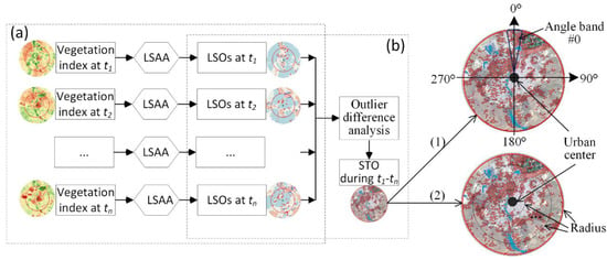
2.3.1. Modeling Framework

We propose a framework of Localized Spatial Association Analysis under Temporal Context, or LSAA-TC, to model the human-induced CUG (H-CUG). Though its application was demonstrated for the Wuhan metropolitan area, LSAA-TC can be similarly applied to any region. Without loss of generality, let A be an attribute domain and A_i,j,k a numerical value of an object O_i,j,k, or referred to as a spatiotemporal space unit, in a 3-D space with dimension size of n × p × q, which is divided into a temporal dimension T(n) and a spatial dimension S(p, q), where T can be broken down into n consecutive but non-overlapping time spans T_i, namely T = {T_i, i = 1, 2, …, n, n ≥ 2}, and S represents a set of locational elements s_j,k (1 ≤ j ≤ p, 1 ≤ k ≤ q) indicating the locations of the n × p × q O_i,j,k elements in a two-dimensional space. Given a specific temporal point t_i in T_i, namely t_i ∈ T_i and t₁ < t₂ < … < t_n (i = 1, 2, …, n), O_i,j,k is labeled as a local spatial outlier (LSO) at time t_i, if A_i,j,k is significantly different (higher or lower) from the values of its neighboring elements defined by a spatial neighborhood size d in S, where H-L will be assigned to O_i,j,k if A_i,j,k is significantly higher than the values of its neighboring elements or L-H assigned to O_i,j,k if A_i,j,k is significantly lower than its neighbors; otherwise, O_i,j,k is labeled as non-outlier. LSOs can be conveniently computed by localized spatial association analysis (LSAA) such as Anselin’s Moran I. A typical method for labeling O_i,j,k using Moran’s scatterplot is outlined by Anselin [47,48]. An LSO layer records all the locations that are labeled as LSO at a temporal point t_i in the 3-D space.

For a given location s_j,k (1 ≤ j ≤ p, 1 ≤ k ≤ q), there are n O_i,j,k objects, each corresponding to time t_i, labeled as either outlier (H-L or L-H) or non-outlier. A spatiotemporal outlier (STO) is defined for location s_j,k if the n O_i,j,k objects (i = 1, 2, …, n, n ≥ 2) located at s_j,k show different LSO patterns (outlier or non-outlier). An STO denotes a point feature in the spatial dimension S(p, q) where significant change in terms of the value of the target variable is observed at least once for the n consecutive periods. The 3-D space filled with a total number of n × p × q (O_i,j,k) objects is input into a process for outlier difference analysis which outputs a point feature layer representing the s_j,k (1 ≤ j ≤ p, 1 ≤ k ≤ q) that are labeled as STO, depending on the LSO patterns of the n O_i,j,k located at s_j,k. When vegetation greenness (e.g., vegetation index derived from remote sensing images) is set as the target variable of interest, the output STOs will indicate the location with an occurrence of significant change in urban greenness. In addition, since LSAA is performed at a local scale, the result indicates the impact on the vegetation abundance from local-scale factors (typically from human activities).

LSAA-TC is a common framework that can be used to map H-CUG. For the particular case studied, the 16 stacked MVC layers defined the temporal dimension for the 3-D space. Two steps were involved in the STO computation from the MVC dataset. First, each of the 16 MVC layers was analyzed using LSAA (e.g., the local Moran’s I, Figure 2a) to extract an LSO layer. In this step, the neighborhood size must be decided [49]. As there is no rule of thumb to determine the optimal size for the neighborhood, queen or rook contiguity is often used in assessing urban ecological quality through a remote sensing dataset [50,51]. Considering the scale of human activities in the city, the size was extended by one more pixel, namely neighborhood distance d = 2, which resulted in 25 elements (5 × 5 pixels) included in each neighborhood, with the distance matrix further row-standardized to give a computational advantage [48]. In the next step, the outliers located at the n periods from the previous one were processed by the outlier difference analysis to find the STO layers (Figure 2b). Depending on the number of periods taken in the computation, both long-term and short-term STOs could be mapped. If all the LSO layers (n = 16 for the case study) from LSAA are analyzed for their outlier differences, a single STO layer, referred to as long-term STO layer, is produced; a long-term STO layer records the locations where significant change in the target variable value (namely, NDVI) is observed during the whole period. If only a subset of the LSO layers, e.g., layers corresponding to any two consecutive times, are analyzed for the outlier differences, then a short-term STO layer is computed for that temporal window (during the time span). Thus, multiple short-term STO layers can be produced depending on the division setting of the whole period. Multiple short-term STO layers, computed by comparing the patterns of the local spatial outlier between any consecutive periods, can provide information of the temporal variance of STOs over a long study period. In the case study, an annual step was decided for deriving the short-term STO layers to reveal the temporal (annual) variations in the H-CUG.

2.3.2. Mapping Spatiotemporal Variations of H-CUG

To map the spatiotemporal patterns of H-CUG, the STO layers (including long-term and short-term) were analyzed from two aspects, including anisotropic characteristics and distance from the urban center (Figure 2c). First, to reveal the possible variations in the anisotropic characteristics, the study region was split into 36 bands and each band represented a 10° cone-shaped sector (angle band hereafter), with the origin set at the urban center (see the right top figure in Figure 2). The first angle band (#0) faced exactly at north (0°) with a 5° band width at each side. Similarly, the second angle band (#1) pointed at 10° relative to the north direction (clockwise) with a 5° band for both sides. Secondly, to reveal the variations related to the distance from the urban center, the ROI was divided into various radius belts with the urban center as the origin. Except the most inner one, which was 0–2 km in radius, all the other belts were equally divided with 1 km in distance to the next (see the right bottom figure in Figure 2; note that not all belts are shown). STO points for both long-term and short-term were analyzed for all the angle bands and the radius belts, respectively.

For each areal unit (i.e., the area given by any angle band or radius belt), the percentage of area that experiences significant urban greenness change (P-A-C), or the density of STO points, could be calculated. Given the spatial resolution (SR) of the multi-temporal imagery dataset from which the STO points are derived, P-A-C is defined,

P-A-C = n × SR²/TA × 100(%),

(1)

where TA is the total area of a considered areal unit, n is the number of STO points within TA, SR is the spatial resolution of the imagery from which the STO points are computed, and SR² and TA have the same unit. Given a spatiotemporal space defined by an areal unit and a time span, P-A-C reflects the level of H-CUG within the space.

2.3.3. Analyzing the Relationship between H-CUG and Land Cover Changes

The short-term STO layers were compared to the land cover changes (LCCs) layers for an identical temporal period. In total, 12 LCC layers were computed through a pixel-by-pixel comparison between any two consecutive years during 2001–2013 from the 13 LCT layers. Considering that the target variable corresponds to the peak vegetation greenness in each year, we expected that LCCs and type conversion among the three LCTs, namely, urban (U), water (W), and others (O), should somehow correlate with the STO events. Direct pixel-by-pixel comparison of LCCs and STOs was not realistic because the spatial resolutions for the two datasets were mismatched (250 m for STO vs 500 m for LCC). Instead, a circle-based co-occurrence resampling method was designed to check the STO-LCC correlation. Specifically, 2500 (50 × 50) points were decided within the bounding envelope of the ROI, with equal distance (2 km) between each neighboring points. Then, the created points were buffered to make non-overlapped circles (radius = 1 km). The circles located within water areas in all the 13 LCT layers and outside ROI were excluded. In the end, 1859 circles were kept, which were used to define the co-occurrence of STO and LCC points if they were in the same circle. The confusion matrix summarizing the co-occurring events of STO and LCC events located within each circle, either true (T) or false (F), was reported.

3. Computing Implementation

The computing implementation of the proposed LSAA-TC framework was composed of two key modules, localized spatial association analysis (LSAA) to extract local spatial outliers (LSOs) for each period and computation of spatiotemporal outliers (STOs) from the LSO data under the temporal context. Automatic modeling and implementation with little human interference can greatly improve the adaptability of the proposed approach. In this case study, a yearly time division was decided as the temporal step. To begin the computation, the start year and the end year were specified. Depending on the input years (start year and end year), a long-term STO layer (2000–2015) and 15 short-term STO layers (annually, 2000–2001, 2001–2002, …, 2014–2015) were computed. ArcGIS model builder (https://www.esri.com) was used to present the tool (model) that automated the extraction of the LSO patterns (outliers or non-outliers).

To extract LSOs for a particular time, several processes were linked in the model (Figure 3). To start, the model loops through the years (or periods, with step set as 1; see the process A in Figure 3) and then the target MVC layer was decided automatically in an iterative manner. Two preconditions, one was the current selected year and the other was the MVC dataset, were affiliated with the MVC layer selection process (process B in Figure 3) which output the selected MVC raster layer for the selected time (year). In order to perform the analysis by taking advantage of Local Moran’s I computation, the selected MVC layer was converted to a vector format (a point layer) through the process C. This point layer was fed into the LSAA (labeled with D, the cluster and outlier analysis) which, in addition to outputting the index value (local Moran’s I) and the corresponding z-score and p-value (probability field), reported LSO patterns (through the field COType). In the end, the spatial outliers were kept, through the process E, to create an LSO layer recording all spatial outliers (H-L or L-H) for the selected year. The process was iterated until all LSO layers for all the years were made ready.

Based on the LSO layers, computing the short-term and long-term STO layers starts with the selection of the input of start time and end time. The following code shows the computing algorithm for the short-term STO layer, with an annual (yearly) temporal step (

Table 1. Short-term (at yearly step) STO layer.

Input: a selected year (input_year) and two LSO layers for the consecutive years (input_year, input_year-1) Output: an STO layer, STOinput_year, with points showing locations of significant change in the target variable (NDVI in this case) during the period from input_year-1 to input_year Algorithm: Create an empty STO layer (STOinput_year) p1: Loop through all georeferenced outlier points (OPi,input_year-1, at location i) in LSOinput_year-1   If the OPi,input_year-1 and OPi,input_year in LSOinput_year do not have an identical spatial outlier label, an STO point at location i is created and appended to STOinput_year End loop p2: Loop through all georeferenced outlier points (OPi,input_year, at location i) in LSOinput_year   If an OPi,input_year and OPi,input_year-1 in LSOinput_year-1 do not have an identical spatial outlier label, an STO point at location i is created and appended to STOinput_year if there is no STO point already created previously End loop

).

The above procedures (p1 and p2) created STO points for each short-term STO layer (STO_{input_year}), representing locations where the LSO patterns (outlier or non-outlier) for the two consecutive years were different. Given that the current study have 16 LSO layers, 15 short-term STO layers were created. Following a similar principle, the long-term STO layer could be computed; alternatively, the long-term STO layer could be computed through a spatial union of all the short-term STO layers. The model and all the computing algorithms were implemented on the ArcGIS platform based on the model builder and Python scripts (https://www.esri.com).

4. Results

4.1. H-CUG Patterns with Respect to Distance from the Urban Center

The spatiotemporal patterns of P-A-C distribution examined from the perspective of the distance to the urban center at an annual step (2000–2015) are illustrated in Figure 4, where the x-axis indicates the distance from the urban center (see Figure 1) and y-axis denotes the division of the temporal span. The result indicates that, for radius belts close to the urban center, very weak H-CUG was detected for most of the years. The result is understandable since a majority of the area in the central urbanized area (downtown area) was categorized as built-up, leaving a very limited space for vegetation cover to convert to or from regardless of possible high intensities of human activities. Conversely, high P-A-C was observed in the range around 5–25 km for most of the years, particularly in the suburban areas between 14 and 20 km, indicating significant changes in urban greenness induced from local-scale impact. It is known that the city experienced significant changes in land cover, particularly urbanization, in the joining part between the urbanized region and the rural areas [6], which may explain why the dominant area showing H-CUG was observed in the suburban regions. When examined from the temporal perspective (y-axis), considerable spatiotemporal variation was observed in the P-A-C distributions. For example, H-CUG showed a highest value in belt 4 (the belt between 3 and 4 km to the urban center) during 2013–2015. Furthermore, the study found that the areas with relatively high P-A-C tended to expand outside from the urban center during the period, starting from the radius belts between 14 and 17 km at the early time to the belts between 17 and 20 km at the end (the red parallelogram in Figure 4). The sensitive H-CUG belts concurred with the urbanization frontier, known as the urban sprawl boundary, which was reported by other studies [40,43]. Remote areas with the radius distance after the urbanization frontier (mostly countryside) were mainly dominated by relatively lower P-A-C, caused by reduced impact on vegetation cover from human activities.

The overall or long-term (LT, during 2000–2015) impact on the urban greenness from human activities was reflected by the change in the P-A-C gradient along the x-axis or the distance from the urban center, as shown at the top bar in Figure 4. The traditional downtown area (roughly 0–4 km from the urban center) generally presented the lowest P-A-C value, and the highest P-A-C values were observed in the radius belts located within 14–20 km (with high H-CUG), which was identical to the short-term P-A-C results.

4.2. H-CUG Patterns with Respect to Orientation

The spatiotemporal P-A-C patterns with respect to the orientation (angle division) are presented in Figure 5. Among the 36 orientation bands (band #0, #1, …, and #35), those centered at #4, #8, #13 and #20–22 exhibited the highest P-A-C values, indicating clearly the anisotropy of the H-CUG distribution. In addition, high P-A-C values showed the temporal variations. For example, the majority of grids with the highest P-A-C values were present in the year of 2003–2004 and 2012–2015. The results suggest heterogeneous patterns observed for the H-CUG in terms of the orientation, which might be related to possible constraints on land use exploitation that the urban infrastructure (and other factors) placed for some activities of human beings [44]. The long-term (LT) P-A-C distribution patterns confirmed the characteristics of the anisotropy in H-CUG, with the highest values located at bands #4, #8, and #22 (dark pink grid at the top side in Figure 5).

The temporal dynamics of H-CUG over the whole region was investigated. The result showed a significant variation in the H-CUG over the years (the green bar at the right side, Figure 5). The P-A-C with values higher than 5% was observed during the years 2002–2004 and after 2008, particularly in the period 2002–2003, 2003–2004 and 2011–2012. The result demonstrates varied levels of H-CUG over the years.

4.3. Relationship between STO and Land Cover Changes

The relationship between STO points and the land cover changes (LCCs, based on the conversion matrix of land cover types between any two consecutive years through MODIS MCD 12Q1) during 2001–2013 is presented based on the circle-based co-occurrence resampling approach. Statistics of the co-occurrence between STO points and land cover changes is summarized in the confusion matrix table from which the kappa value was computed (with examples given for the periods 2002–2003 and 2008–2009, in Figure 6). The result indicates that the kappa value for most of the years was over 0.20, suggesting that STO points and the locations corresponding to land cover changes were fairly associated. Thus, the land cover changes and STO events may provide mutual explanation to some extent, but there are also some other factors not included.

5. Discussions

5.1. Advantage and Rationality of LSAA-TC

The current study demonstrates the work of exploring the spatiotemporal patterns of H-CUG through a modeling framework named Localized Spatial Association Analysis under Temporal Context (LSAA-TC). With the outputs of STOs and P-A-C, LSAA-TC maps the distribution of the changes in urban greenness induced from local-scale impacts, primarily from human activities. Vegetation cover is important for improving climate conditions and building a comfortable habitat for human beings in urbanized areas [19,52]. Rapid urbanization in many parts of the world during the last few decades has led to significant changes in vegetation space, due to the shrinkage of vegetation space as more vegetation cover converted into other land use types (e.g., built-up) [9]. Therefore, understanding the changes in vegetation distribution and abundance, particularly due to human activities, can help design sound land-use policies promoting harmonious human–natural environment relationship. A few approaches have been proposed to map vegetation cover changes. For example, through subtraction analysis in vegetation index (SAVI) over a certain period, the health of a vegetation cover can be reflected by the difference between the start and end of the period. However, SAVI is a pixel-based approach that is unable to separate the impact on vegetation cover from local-scale factors (mainly human activities) and from large scale factors (regional influences such as climatic changes) [53]. Moreover, the direct comparison of the pixel values (e.g., NDVI) between the periods through SAVI method may suffer critical uncertainty due to the inconsistency in the sensitivity of the sensor during image acquisition at different times. LSAA-TC applies localized spatial association analysis (LSAA) and the mapped H-CUG result is insensitive to possible inconsistency in the sensor sensitivity at different times.

The assumption underlying LSAA-TC is that the climatic factors (e.g., the fluctuations in rainfall and temperature) affect the vegetation cover over a large extent (large scale) while the impact on urban greenness from local-scale factors, typically human activities (e.g., land exploitation), tends to cause a fragmentation of vegetation cover (landscape heterogeneity) within a short period (e.g., a few months or within a year). The fragmentation of landscapes due to human activities has been long recognized [54]. Human activities can cause environmental changes and fragment habitats via the conversion of land use types [55]. Paul and Nagendra [56] found that a high proportion of vegetation fragmentation in the city core was triggered by human activities (e.g., infrastructural expansion). To characterize landscape fragmentation, Fan and Myint [57] state that the utility of local-scale association indices derived directly from satellite imagery is superior to generating and employing detailed land cover classification maps. Even though the local-scale spatial pattern analysis (e.g., LSAA) is essentially a static method that only captures LSO patterns (outlier or non-outlier) at a single temporal point, it carries no information for unveiling the changes in the variable of interest (e.g., urban greenness). To map H-CUG, the proposed LSAA-TC attempts to compare the changes of local-scale distribution patterns in urban greenness under the temporal context. The computed STO density, or P-A-C, reveals locations where H-CUG happened. Furthermore, the analytical processes could be automated so that mapping H-CUG is convenient to implement.

Though the assumption for LSAA-TC may hold for the majority of cases, it can still be challenged by the fact that vegetation could also be affected by microclimatic factors [58], or conversely, large-scale restoration programs [59]. Nevertheless, as long as the microclimatic factors are stable over a period of years, their impact on vegetation will not be detected in the result of the H-CUG. Further, areas that experienced large-scale restoration can be easily located and dug out before the analysis. Thus, the results from the computed H-CUG could illustrate the changes in urban greenness due to local-scale impact, and may serve as an indicator of intensity level that human activities impose on vegetation cover.

5.2. Urban Greenness, Land Cover, and STO

Land cover changes and human activities are closely correlated in urban ecosystems [17]. Land cover is composed of vegetation and non-vegetated types. Building a land cover conversion matrix (LCCM) at the start and end of a time period is a useful way to quantify the changes in vegetation cover over the period, since vegetation cover could be transformed to or from non-vegetated cover types. However, numerous limitations of land cover classification indicate that the utilization of classified thematic maps in landscape pattern analysis is questionable and may even lead to large errors in subsequent analyses [57]. Moreover, the LCCM method alone is insufficient in quantifying urban greenness changes. For example, tree removal or transplantation might not update land cover types, but is likely to induce significant change in vegetation density (reflected by the vegetation index) [60], leading to the detection of an STO event but not the conversion of land cover types. LSAA-TC extracts local spatial outliers and computes spatiotemporal outliers directly from satellite imagery. The spatiotemporal patterns of H-CUG are revealed by the STO layers.

The current study indicates that the relationship between the STO points and land cover changes (LCCs) was somehow correlated but not strong enough for their mutual explanation, namely, LCCs could only partially explain the STOs and vice versa (see Figure 6). The underlying reason may be manifold. Some factors could incur STO points but do not necessarily lead to the conversion of land cover types. Similarly, land cover type conversion (e.g., from grassland to farmland) may not necessarily mean significant changes in urban greenness and thus STO points cannot be inferred. Based on the relationship between LCCs and STOs, it is appropriate to conclude that LSAA-TC is useful for detecting changes in urban greenness at a local scale but not suitable for mapping the conversion in land cover types. Conversely, mapping the conversions of land cover types alone is insufficient to understand the changes in urban greenness.

5.3. Scale Consideration in LSAA-TC

The importance of scale in LSAA-TC can be examined from two aspects. First, the created STOs are the overall representation of the changes in urban greenness associated with the mixed effect from the fraction of vegetated land cover and other land cover types, known as endmembers [19]. Urban land cover is often highly fragmented as the result of the long-term interactions from natural and anthropogenic factors, which leads to a high within-class variance or mixed-pixel problem for many mapped land cover units [19,61,62]. Xian et al. [63] stated that a single pixel in remote sensing imagery in urban areas is often mixed and composed of several land-cover/land-use types. Such a mixing property in pixels is even more common for imagery with a coarse resolution. Thus, an STO point represents the location/pixel experiencing significant changes of the overall vegetation abundance contributed by various land cover types. Second, the resultant STOs can be affected by the spatial scale of the remote sensing data adopted in the analysis. Depending on the economic development of the study region, the term local scale, as opposed to large scale, may vary from a few meters to a few kilometers. One challenge facing the application of LSAA-TC is the decision for the resolution of the input image product. In general, the impact on land cover from human activities in small cities may be present at a smaller extent than that in large cities, because the urbanization progress, and thus the scale of the changes of urban greenness, varies among cities at the same temporal span (e.g., at an annual step). In a metropolitan city like Wuhan city, the MODIS 13Q1 data with spatial resolution at 250 m might be appropriate to map H-CUG, considering its development level of the city in the recent decade or two. The current study applied an annually temporal step/period to compute the STOs. This decision was based on the adopted spatial resolution (namely, 250 m of MODIS MCD12Q1 dataset) and consideration of the vegetation growing cycle (i.e., annual cycle). However, for small cities, the applied remotely-sensed dataset should be at a finer spatial scale and/or a shorter temporal scale for successful detection of the STO points. Additionally, the neighborhood size is also an important parameter to consider in the local spatial association analysis. The neighborhood size can be estimated based on the global spatial autocorrelation analysis of the vegetation index, which determines a distance range within which spatial correlation may exist. Depending on characteristics of the urban landscape fragmentation, such a range may vary over space and time [56,57]. For the current study, a small local space equivalent to a 5 × 5 (1.25 km × 1.25 km) window proved to be the neighborhood that presented the strongest correlation in terms of urban vegetation for most of the years, thus it might be appropriate for the local spatial association analysis.

A single spatial scale may not be sufficient to detect H-CUG, typically in scenarios where there is a critical inconsistency between the actual scale of the urban greenness changes and the scale of the dataset (imagery resolution) adopted in the analysis. For example, large-scale changes in urban greenness might be missed out if LSAA-TC is performed at a spatial scale that is too small compared to the actual changing extent; conversely, small-scale changes could be too weak to be detected if a large-scale dataset (too coarse imagery) is adopted. The issue of the scale difference imposes a common difficulty for estimating the impact on urban greenness from human-induced factors. To adequately detect the STO points, multi-scale analysis should be applied in future study. The benefit of multi-scale mapping is that each scale is sensitive to H-CUG at a particular spatial resolution and all the STO points detected from various scales can be combined to show the overall H-CUG. However, satellite imagery with high spatial/temporal resolutions must be available for multi-scale H-CUG mapping, which is not always satisfied in satellite imagery applications [22].

5.4. Possible Explanations for STO

Vegetation changes can be attributed to climate variations and human activities [33]. Given the two-step analytical processes involved in LSAA-TC, it is reasonable to conclude that the patterns shown in the STOs denote the impact on urban greenness mainly from human activities. In the case study, the long-term STO events, as shown in Figure 7, illustrates the uneven mode of STO patterns in three belts (circles with the origin at the urban center). For the innermost area (within the belt located between radius 0–5 km, labeled as R₁), there were very limited STO points. Then the belt with further distance from the urban center (between R₁ and R₂, or radius 5–22 km) presented much denser STO points, suggesting a higher probability of H-CUG in this region. This finding is basically consistent with other studies stating that the connecting area between urbanized and rural regions undertook the most frequent land exploitation [42,43,62]. The third belt, beyond the radius R₂, was again characterized by relatively low STO points because the rural area was less affected by human activities.

The changes in water bodies and rivers due to human activities explained most STO points (see the ellipses labeled as S1, S2, and S3 in Figure 7), while other features, including the distribution of transportation (roads and railways) and suburban centers, did not explain many changes in the urban greenness. The significant changes in urban greenness close to water bodies and rivers probably resulted from the vast construction of buildings (real estate development and storage warehouse) close to the river banks or water body borders for a better living environment. It was reported that the urban sprawl and alteration of surface land to agricultural or urban functions have brought about critical shrinkage of surface water area in the city. For example, it was found that the dominant change around the Shahu Lake, one of the principal inner lakes of the city, was lake and vegetation shrinkage [40]. In addition, inter-annual soil moisture change in areas close to water bodies was most significant in different years, which may contribute to the significant intertemporal changes in urban greenness. Transportation infrastructure was reported to have associated with the urbanization process [44,64]; however, the changes in urban greenness seem not to be directly related to the transportation systems. Still, though the suburban centers are important for local residents, their impact on the urban greenness seems to be not as strong as expected. There are other factors that may impose a significant impact on land use and land cover, which was reflected in the distribution of the H-CUG. One of the factors is from land use policies and urban planning, which legally define the freedom level for land use conversion and conversion directions by delimitating red and green patches (areal patches) [42]. For example, the district Dongxihu (roughly the area of the eclipse labeled S4, Figure 7) was designed as a key development region [62], providing more space for free land use conversions by the local government, and therefore high STO density was observed. Furthermore, many other factors may present spatial heterogeneity in terms of the impact on H-CUG. Given more data variables related to urbanization, such as distributions of commercial centers or residential areas, the contribution from those variables may be included to explain the H-CUG patterns based on some advanced spatial models.

5.5. Uncertainties in the Model

Uncertainty is an inherent characteristic of geodata, which could be related to various aspects [65]. Certain uncertainties in the current study need to be addressed. There are several aspects that may introduce uncertainties in the modeled results for H-CUG. First, the MODIS image dataset, MODIS 13Q1, was used to extract the LSO patterns from vegetation cover. Though the image product itself has undergone a series of data preprocessing steps, including geometric and radiometric calibrations, to improve its quality, some uncertainties are possibly still introduced [66]. For example, although the maximum value composite approach (MVC) takes the maximum digital number (DN) from a set of scenes collected at different times, the ultimate result still may suffer from a quality issue. Furthermore, the MODIS imagery (MOD13Q1, including the scenes of DOY 209 and DOY 225) is also known for its coarse spatial resolution, which may present a mixed-pixel issue in the local-scale impact analysis. Thus, the extracted LSO patterns might contain a noisy result. We expect that higher quality remote sensing dataset will improve the analyzed result. In addition it is possible to apply finer scale greenness mapping in the future, as discussed previously, to minimize the impact from the mixed-pixel issue. Second, as discussed previously, the adopted spatiotemporal scales could be inconsistent with the actual detectible spatiotemporal resolutions in the urban greenness changes, which may result in H-CUG not being captured. We suggest that multiple-scale H-CUG maps be extracted and combined together if multi-scale datasets are available.

6. Conclusions

Our study demonstrated that the proposed LSAA-TC could be a promising tool for mapping the spatiotemporal patterns of H-CUG. Computationally, LSAA-TC is consisted in two steps and takes input of multi-temporal vegetation index products inversed from remote sensing images. The first step of LSAA-TC applies localized spatial association analysis (LSAA) to extract local spatial outliers (LSOs). In this step, LSAA performs a clustering analysis such that areas showing outlier concentrations for a target variable of interest could be outputted. The next step examines the multi-temporal LSOs under the temporal context and derives the spatiotemporal outliers (STOs) corresponding to locations experienced significant H-CUG. Urban vegetation plays a key role in urban ecosystem services. The findings of H-CUG patterns from LSAA-TC can shed some helpful insight for understanding the human-induced changes in urban vegetation and provide useful information for urban planning. Furthermore, spatiotemporal variations in H-CUG can be conveniently computed based on LSAA-TC. The case study in Wuhan metropolitan area clearly revealed such variations. For example, the most prominent H-CUG appeared in the rural–urban joint areas and along the borders of the water bodies; thus particular attention should be paid to those areas in land use planning. The work concludes that LSAA-TC is a widely applicable and easy-to-implement framework for mapping the H-CUG patterns, and it is valuable for assisting urban planning. The future study shall concentrate on validating LSAA-TC on more cities at varied development stages and investigate the scale effect on mapping H-CUG based on multi-scale datasets.

References

1. Cohen, B. Urbanization in developing countries: Current trends, future projections, and key challenges for sustainability. Technol. Soc. 2006, 28, 63–80. [Google Scholar] [CrossRef]
2. Guan, X.; Wei, H.; Lu, S.; Dai, Q.; Su, H. Assessment on the urbanization strategy in China: Achievements, challenges and reflections. Habitat Int. 2018, 71, 97–109. [Google Scholar] [CrossRef]
3. Han, H.; Hawken, S. Introduction: Innovation and identity in next-generation smart cities. City Cult. Soc. 2018, 12, 1–4. [Google Scholar] [CrossRef]
4. Itoh, R. Dynamic control of rural-urban migration. J. Urban Econ. 2009, 66, 196–202. [Google Scholar] [CrossRef]
5. Li, H.; Wu, Y.; Huang, X.; Sloan, M.; Skitmore, M. Spatial-temporal evolution and classification of marginalization of cultivated land in the process of urbanization. Habitat Int. 2017, 61, 1–8. [Google Scholar] [CrossRef]
6. Zeng, C.; Liu, Y.; Stein, A.; Jiao, L. Characterization and spatial modeling of urban sprawl in the Wuhan Metropolitan Area, China. Int. J. Appl. Earth Obs. 2005, 34, 10–24. [Google Scholar] [CrossRef]
7. Crum, S.M.; Shiflett, S.A.; Jenerette, G.D. The influence of vegetation, mesoclimate and meteorology on urban atmospheric microclimates across a coastal to desert climate gradient. J. Environ. Manag. 2017, 200, 295–303. [Google Scholar] [CrossRef] [PubMed]
8. Klingberg, J.; Broberg, M.; Strandberg, B.; Thorsson, P.; Pleijel, H. Influence of urban vegetation on air pollution and noise exposure—A case study in Gothenburg, Sweden. Sci. Total Environ. 2017, 599–600, 1728–1739. [Google Scholar] [CrossRef] [PubMed]
9. Dallimer, M.; Tang, Z.; Bibby, P.R.; Brindley, P.; Gaston, K.J.; Davies, Z.G. Temporal changes in greenspace in a highly urbanized region. Biol. Lett. 2011, 7, 763–766. [Google Scholar] [CrossRef] [PubMed] [Green Version]
10. Lu, Y.; Coops, N.C.; Hermosilla, T. Estimating urban vegetation fraction across 25 cities in pan-Pacific using Landsat time series data. ISPRS J. Photogramm. Remote Sens. 2017, 126, 11–23. [Google Scholar] [CrossRef]
11. Pullanikkatil, D.; Palamuleni, L.; Ruhiiga, T. Land use/land cover change and implications for ecosystems services in the Likangala River Catchment, Malawi. Phys. Chem. Earth 2016, 93, 96–103. [Google Scholar] [CrossRef]
12. Tao, Y.; Wang, H.; Ou, W.; Guo, J. A land-cover-based approach to assessing ecosystem services supply and demand dynamics in the rapidly urbanizing Yangtze River Delta region. Land Use Policy 2018, 72, 250–258. [Google Scholar] [CrossRef]
13. Chen, Y.; Shi, P.; Li, X.; Chen, J.; Li, J. A combined approach for estimating vegetation cover in urban/suburban environments from remotely sensed data. Comput. Geosci. 2006, 32, 1299–1309. [Google Scholar]
14. Morris, K.; Chan, A.; Ooi, M.; Oozeer, M.; Abakr, Y.; Morris, K. Effect of vegetation and waterbody on the garden city concept: An evaluation study using a newly developed city, Putrajaya, Malaysia. Comput. Environ. Urban Syst. 2016, 58, 39–51. [Google Scholar] [CrossRef]
15. Naeem, S.; Cao, C.; Waqar, M.M.; Wei, C.; Acharya, B.K. Vegetation role in controlling the ecoenvironmental conditions for sustainable urban environments: A comparison of Beijing and Islamabad. J. Appl. Remote Sens. 2018, 12, 016013. [Google Scholar] [CrossRef]
16. Li, S.; Sun, Z.; Tan, M.; Li, X. Effects of rural–urban migration on vegetation greenness in fragile areas: A case study of Inner Mongolia in China. J. Geogr. Sci. 2016, 26, 313–324. [Google Scholar] [CrossRef] [Green Version]
17. Wang, Z.; Yang, S.; Wang, S.; Shen, Y. Monitoring evolving urban cluster systems using DMSP/OLS nighttime light data: A case study of the Yangtze River Delta region, China. J. Appl. Remote Sens. 2017, 11, 046029. [Google Scholar] [CrossRef]
18. Emmanuel, R. Urban vegetational change as an indicator of demographic trends in cities: The case of Detroit. Environ. Plan. B Plan. Des. 1997, 24, 415–426. [Google Scholar] [CrossRef]
19. Gan, M.; Deng, J.; Zheng, X.; Hong, Y.; Wang, K. Monitoring Urban Greenness Dynamics Using Multiple Endmember Spectral Mixture Analysis. PLoS ONE 2014, 9, e112202. [Google Scholar] [CrossRef] [PubMed]
20. Anchang, J.; Ananga, E.; Pu, R. An efficient unsupervised index based approach for mapping urban vegetation from IKONOS imagery. Int. J. Appl. Earth Obs. 2016, 50, 211–220. [Google Scholar] [CrossRef]
21. Shi, D.; Yang, X. Mapping vegetation and land cover in a large urban area using a multiple classifier system. Int. J. Remote Sens. 2017, 38, 4700–4721. [Google Scholar] [CrossRef]
22. Tan, M. An Intensity Gradient/Vegetation Fractional Coverage Approach to Mapping Urban Areas From DMSP/OLS Nighttime Light Data. IEEE J. Sel. Top. Appl. Earth Observ. Remote Sens. 2016, 10, 95–103. [Google Scholar] [CrossRef]
23. Grubesic, T.H.; Wallace, D.; Chamberlain, A.W.; Nelson, J.R. Using unmanned aerial systems (UAS) for remotely sensing physical disorder in neighborhoods. Landsc. Urban Plan. 2018, 169, 148–159. [Google Scholar] [CrossRef]
24. Xie, Y.; Sha, Z.; Yu, M. Remote sensing imagery in vegetation mapping: A review. J. Plant Ecol. 2008, 1, 9–23. [Google Scholar] [CrossRef]
25. Oldeland, J.; Dorigo, W.; Lieckfeld, L.; Lucieer, A.; Jürgens, N. Combining vegetation indices, constrained ordination and fuzzy classification for mapping semi-natural vegetation units from hyperspectral imagery. Remote Sens. Environ. 2010, 114, 1155–1166. [Google Scholar] [CrossRef]
26. Wang, Z.; Wang, T.; Darvishzadeh, R.; Skidmore, A.K.; Jones, S.; Suarez, L.; Woodgate, W.; Heiden, U.; Heurich, M.; Hearne, J. Vegetation indices for mapping canopy foliar nitrogen in a mixed temperate forest. Remote Sens. 2016, 8, 491. [Google Scholar] [CrossRef]
27. Igamberdiev, R.M.; Bill, R.; Schubert, H.; Lennartz, B. Analysis of cross-seasonal spectral response from kettle holes: Application of remote sensing techniques for chlorophyll estimation. Remote Sens. 2012, 4, 3481–3500. [Google Scholar] [CrossRef]
28. Defries, R.S.; Townshend, J.R. Ndvi-Derived Land Cover Classifications At a Global Scale. Int. J. Remote Sens. 1994, 15, 3567–3586. [Google Scholar] [CrossRef]
29. Fan, X.; Liu, Y. A global study of NDVI difference among moderate-resolution satellite sensors. ISPRS J. Photogramm. Remote Sens. 2016, 121, 177–191. [Google Scholar] [CrossRef]
30. Li, Y.; Chen, S.; Yan, Y.; Yu, C. Effects of urbanization on vegetation degradation in the Yangtze River Delta of China: Assessment based on SPOT-VGT NDVI. J. Urban Plan. Dev. 2014, 141, 1–11. [Google Scholar] [CrossRef]
31. Zhang, H.K.; Roy, D.P. Using the 500 m MODIS land cover product to derive a consistent continental scale 30 m Landsat land cover classification. Remote Sens. Environ. 2017, 197, 15–34. [Google Scholar] [CrossRef]
32. Fenta, A.A.; Yasuda, H.; Haregeweyn, N.; Belay, A.S.; Hadush, Z.; Gebremedhin, M.A.; Mekonnen, G. The dynamics of urban expansion and land use/land cover changes using remote sensing and spatial metrics: The case of Mekelle city of northern Ethiopia. Int. J. Remote Sens. 2017, 38, 4107–4129. [Google Scholar] [CrossRef]
33. Solins, J.P.; Thorne, J.H.; Cadenasso, M.L. Riparian canopy expansion in an urban landscape: Multiple drivers of vegetation change along headwater streams near Sacramento, California. Landsc. Urban Plan. 2018, 172, 37–46. [Google Scholar] [CrossRef]
34. Markovchicknicholls, L.; Regan, H.M.; Deutschman, D.H.; Widyanata, A.; Martin, B.; Noreke, L.; Hunt, T.A. Relationships between human disturbance and wildlife land use in urban habitat fragments. Conserv. Biol. 2008, 22, 99–109. [Google Scholar] [CrossRef] [PubMed]
35. Van der Walt, L.; Cilliers, S.S.; Kellner, K.; Du Toit, M.J.; Tongway, D. To what extent does urbanisation affect fragmented grassland functioning? J. Environ. Manage. 2015, 151, 517–530. [Google Scholar] [CrossRef] [PubMed]
36. Evans, J.; Geerken, R. Discrimination between Climate and Human Induced Dryland Degradation. J. Arid Environ. 2004, 57, 535–554. [Google Scholar] [CrossRef]
37. Li, A.; Wu, J.; Huang, J. Distinguishing between human-induced and climate-driven vegetation changes: A critical application of RESTREND in inner Mongolia. Landsc. Ecol. 2012, 27, 969–982. [Google Scholar] [CrossRef]
38. Small, C.; Lu, J.W.T. Estimation and vicarious validation of urban vegetation abundance by spectral mixture analysis. Remote Sens. Environ. 2006, 100, 441–456. [Google Scholar] [CrossRef]
39. De la Barrera, F.; Henriquez, C. Vegetation cover change in growing urban agglomerations in Chile. Ecol. Indic. 2017, 81, 265–273. [Google Scholar] [CrossRef]
40. He, Q.; Tan, R.; Gao, Y.; Zhang, M.; Xie, P.; Liu, Y. Modeling urban growth boundary based on the evaluation of the extension potential: A case study of Wuhan city in China. Habitat Int. 2018, 72, 57–65. [Google Scholar] [CrossRef]
41. Cheng, J.; Masser, I. Urban growth pattern modelling: A case study of Wuhan city, PR China. Landsc. Urban Plan. 2003, 62, 199–217. [Google Scholar] [CrossRef]
42. Zeng, C.; Zhang, A.; Xu, S. Urbanization and administrative restructuring: A case study on the Wuhan urban agglomeration. Habitat Int. 2016, 55, 46–57. [Google Scholar] [CrossRef] [Green Version]
43. Hu, S.; Tong, L.; Frazier, A.; Liu, Y. Urban boundary extraction and sprawl analysis using Landsat images: A case study in Wuhan, China. Habitat Int. 2015, 47, 183–195. [Google Scholar] [CrossRef] [Green Version]
44. Tan, R.; Liu, Y.; Liu, Y.; He, Q.; Ming, L.; Tang, S. Urban growth and its determinants across the Wuhan urban agglomeration, central China. Habitat Int. 2014, 44, 268–281. [Google Scholar] [CrossRef]
45. Qin, Y.; Xiao, X.; Dong, J.; Zhou, Y.; Wang, J.; Doughty, R.; Chen, Y.; Zou, Z.; Moore, B. Annual dynamics of forest areas in South America during 2007–2010 at 50-m spatial resolution. Remote Sens. Environ. 2017, 201, 73–87. [Google Scholar] [CrossRef]
46. Zeng, T.; Zhang, Z.; Zhao, X.; Wang, X.; Zuo, L. Evaluation of the 2010 MODIS Collection 5.1 Land Cover Type Product over China. Remote Sens. 2015, 7, 1981–2006. [Google Scholar] [CrossRef] [Green Version]
47. Anselin, L. Local Indicators of Spatial Association—LISA. Geogr. Anal. 1995, 27, 93–115. [Google Scholar] [CrossRef]
48. Fischer, M.; Scholten, H.; Unwin, D. Spatial Analytical Perspectives on GIS, 3rd ed.; Taylor and Francis: London, UK, 1996; pp. 111–125. [Google Scholar]
49. Bone, C.; Wulder, M.; White, J.; Robertson, C.; Nelson, T. A GIS-Based Risk Rating of Forest Insect Outbreaks Using Aerial Overview Surveys and the Local Moran’s I Statistic. Appl. Geogr. 2013, 40, 161–170. [Google Scholar] [CrossRef]
50. Hu, X.; Xu, H. A new remote sensing index for assessing the spatial heterogeneity in urban ecological quality: A case from Fuzhou City, China. Ecol. Indic. 2018, 89, 11–21. [Google Scholar] [CrossRef]
51. Murray, A.; Grubesic, T.; Wei, R. Spatially significant cluster detection. Spat. Stat. 2014, 10, 103–116. [Google Scholar] [CrossRef]
52. Dennis, M.; Barlow, D.; Cavan, G.; Cook, P.; Gilchrist, A.; Handley, J.; James, P.; Thompson, J.; Tzoulas, K.; Wheater, C.P.; Lindley, S. Mapping Urban Green Infrastructure: A Novel Landscape-Based Approach to Incorporating Land Use and Land Cover in the Mapping of Human-Dominated Systems. Land 2018, 7, 17. [Google Scholar] [CrossRef]
53. Mancino, G.; Nolè, A.; Ripullone, F.; Ferrara, A. Landsat TM imagery and NDVI differencing to detect vegetation change: Assessing natural forest expansion in Basilicata, southern Italy. IForest 2014, 7, 75–84. [Google Scholar] [CrossRef]
54. Pueyo, Y.; Alados, C.; Barrantes, O. Determinants of Land Degradation and Fragmentation in Semiarid Vegetation at Landscape Scale. Biodivers. Conserv. 2006, 15, 939–956. [Google Scholar] [CrossRef]
55. Tilman, D.; Lehman, C. Human-caused environmental change: Impacts on plant diversity and evolution. Proc. Natl. Acad. Sci. USA 2001, 98, 5433–5440. [Google Scholar] [CrossRef] [PubMed] [Green Version]
56. Paul, S.; Nagendra, H. Vegetation change and fragmentation in the mega city of Delhi: Mapping 25 years of change. Appl. Geogr. 2015, 58, 153–166. [Google Scholar] [CrossRef]
57. Fan, C.; Myint, S. A comparison of spatial autocorrelation indices and landscape metrics in measuring urban landscape fragmentation. Landsc. Urban Plan. 2014, 121, 117–128. [Google Scholar] [CrossRef]
58. Lehmann, I.; Mathey, J.; Rößler, S.; Bräuer, A.; Goldberg, V. Urban vegetation structure types as a methodological approach for identifying ecosystem services—Application to the analysis of micro-climatic effects. Ecol. Indic. 2014, 42, 58–72. [Google Scholar] [CrossRef]
59. Fu, W.; Lu, Y.; Harris, P.; Comber, A.; Wu, L. Peri-urbanization may vary with vegetation restoration: A large scale regional analysis. Urban For. Urban Green. 2018, 29, 77–87. [Google Scholar] [CrossRef]
60. Bottalico, F.; Chirici, G.; Giannetti, F.; De Marco, A.; Nocentini, S.; Paoletti, E.; Salbitano, F.; Sanesi, G.; Serenelli, C.; Travaglini, D. Air Pollution Removal by Green Infrastructures and Urban Forests in the City of Florence. Agric. Agric. Sci. Procedia 2016, 8, 243–251. [Google Scholar] [CrossRef]
61. Rosentreter, J.; Hagensieker, R.; Okujeni, A.; Roscher, R.; Wagner, P.D.; Waske, B. Subpixel Mapping of Urban Areas Using EnMAP Data and Multioutput Support Vector Regression. IEEE J. Sel. Top. Appl. Earth Obs. Remote Sens. 2017, 10, 1938–1948. [Google Scholar] [CrossRef]
62. Chen, Z.; Zhang, A.; Song, M.; Zhang, Z. Measuring external costs of rural–urban land conversion: An empirical study in Wuhan, China. Acta Ecol. Sin. 2016, 36, 30–35. [Google Scholar] [CrossRef]
63. Xian, G.; Yang, L.; Klaver, J.M. Urban Land-Cover Change Detection through Sub-Pixel Imperviousness Mapping Using Remotely Sensed Data. Photogramm. Eng. Remote Sens. 2003, 69, 1003–1010. [Google Scholar]
64. Guan, X.; Lin, X.; Shilin, H.U.; Shasha, L.U. Relationship between transportation system and urban spatial expansion in Wuhan Urban Agglomeration. Prog. Geogr. 2014, 33, 702–712. [Google Scholar]
65. Kinkeldey, C.; Schiewe, J.; Gerstmann, H.; Götze, C.; Kit, O.; Lüdeke, M.; Taubenböck, H.; Wurm, M. Evaluating the use of uncertainty visualization for exploratory analysis of land cover change: A qualitative expert user study. Comput. Geosci. 2015, 84, 46–53. [Google Scholar] [CrossRef] [Green Version]
66. Zheng, Z.; Zhu, W. Uncertainty of remote sensing data in monitoring vegetation phenology: A comparison of MODIS C5 and C6 vegetation index products on the Tibetan Plateau. Remote Sens. 2017, 9, 1288. [Google Scholar] [CrossRef]
Figure 1. Location of Wuhan metropolitan area and the region of interest (ROI) defined as the circle with a radius of 50 km originating from the urban center. (a) The location of Hubei province, (b) the boundary of the province, (c) Wuhan city boundary and the ROI, (d) comparison of the NDVI map for the years 2005 and 2015, and (e) three-class land cover types (LCT) showing water (W), urban land (U), and the others (O).
Ijgi 07 00407 g001
Figure 2. Conceptual framework of Localized Spatial Association Analysis under Temporal Context: (a) local spatial outlier (LSO) layer extracted for n temporal periods through localized spatial association analysis (LSAA), (b) spatiotemporal outliers (STOs) computed from LSO layers through an outlier difference analysis, and (c) the spatial variations of the STOs (short-term and long-term) through (1) the 36 direction divisions (only the first band#0 illustrated, the right top figure), and (2) 44 radius divisions (only three radius divisions are given as examples, see the right bottom figure). In this case study, an STO layer was called short-term if n = 2 (for any two consecutive years) or long-term if n = 16 (for the whole period, namely, during 2000–2015).
Ijgi 07 00407 g002
Figure 3. Workflow of the built model for the computing local spatial outliers based on the processed MVC layers computed from the remote sensing dataset MOD13Q1.
Ijgi 07 00407 g003
Figure 4. Grids showing the distribution of percentage of area with significant urban greenness Change (P-A-C), presented for radius belts having various distance from the urban center at different temporal times, where the x-axis shows the radius division and the y-axis shows the temporal span. Long-term (LT) P-A-C (full time span, during 2000–2015) is shown in the grids (in red) at the top side. The parallelogram illustrates the aggregated spatiotemporal region having relatively high P-A-C values. Note that each grid in the figure may represent different area, as their distance to the urban center varies.
Ijgi 07 00407 g004
Figure 5. Grids showing the distribution of percentage of area urban greenness change (P-A-C) defined by the angle bands (totally 36 divisions, originating from the urban center) and temporal spans, where the x-axis shows the angle bands (#0, #1, …, and #35) and the y-axis shows the temporal divisions (2000–2001, 2001–2002, …, 2014–2015). The relatively high P-A-C bands are delineated by the red rectangles. Long-term (LT) P-A-C (the full time span, during 2000–2015) is shown in red grids for each angle band at the top side. The green grids at the right side shows the short-term P-A-C for the entire ROI (without angle/radius division). Note that each grid in the figure may have different area, as their distance to the urban center varies.
Ijgi 07 00407 g005
Figure 6. Confusion matrix for testing the co-occurrence between spatiotemporal outliers (STOs) and land cover changes (LCCs), through a circle-based co-occurrence resampling method: (a) all the resampling circles, (b) the distribution of STOs and LCCs in each period (2000–2001, 2001–2002, …, and 2012–2013, with examples during 2002–2003 and 2008–2009 given), and (c) the confusion matrix of the co-occurrence between LCC and STO events after overlaying (a) and (b), with examples given for periods 2002–2003 and 2008–2009, and the kappa curve for all the periods.
Ijgi 07 00407 g006
Figure 7. Variations of the long-term STO event distribution examined through three circular radii originating from the urban center. The densely populated STOs were mainly located in the belt between R1 and R2. Examples of four delineated patches having densely populated STOs are shown (labels S1, S2, and S3, which are close to water bodies/river, and S4 which is a rapid economic development area thanks to the result from special land plan policies).
Ijgi 07 00407 g007