Comparison of Landscape Metrics for Three Different Level Land Cover/Land Use Maps

 ,
, 
Abstract
1. Introduction
2. Study Area and Data
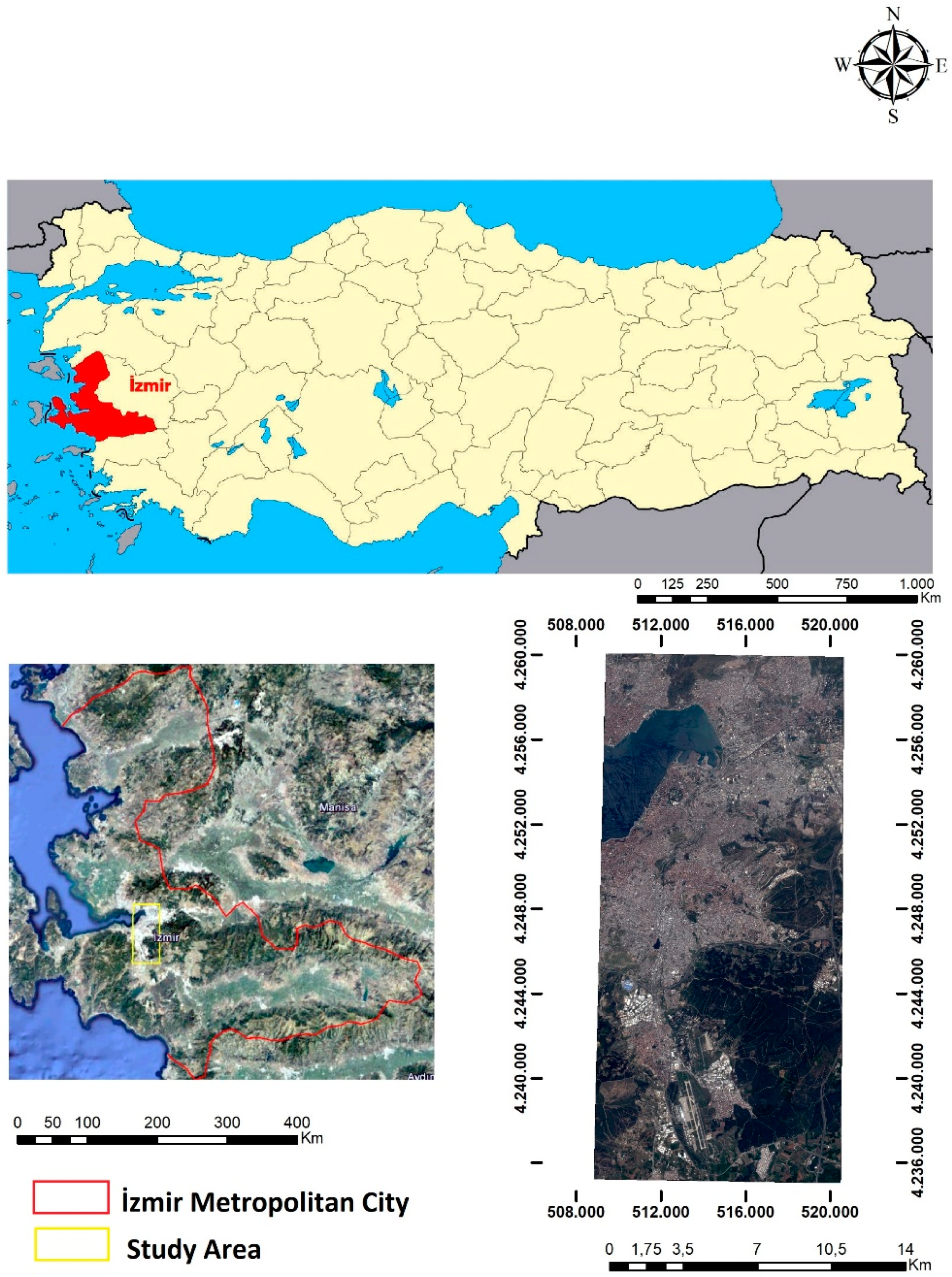
2.1. Study Area
2.2. Data
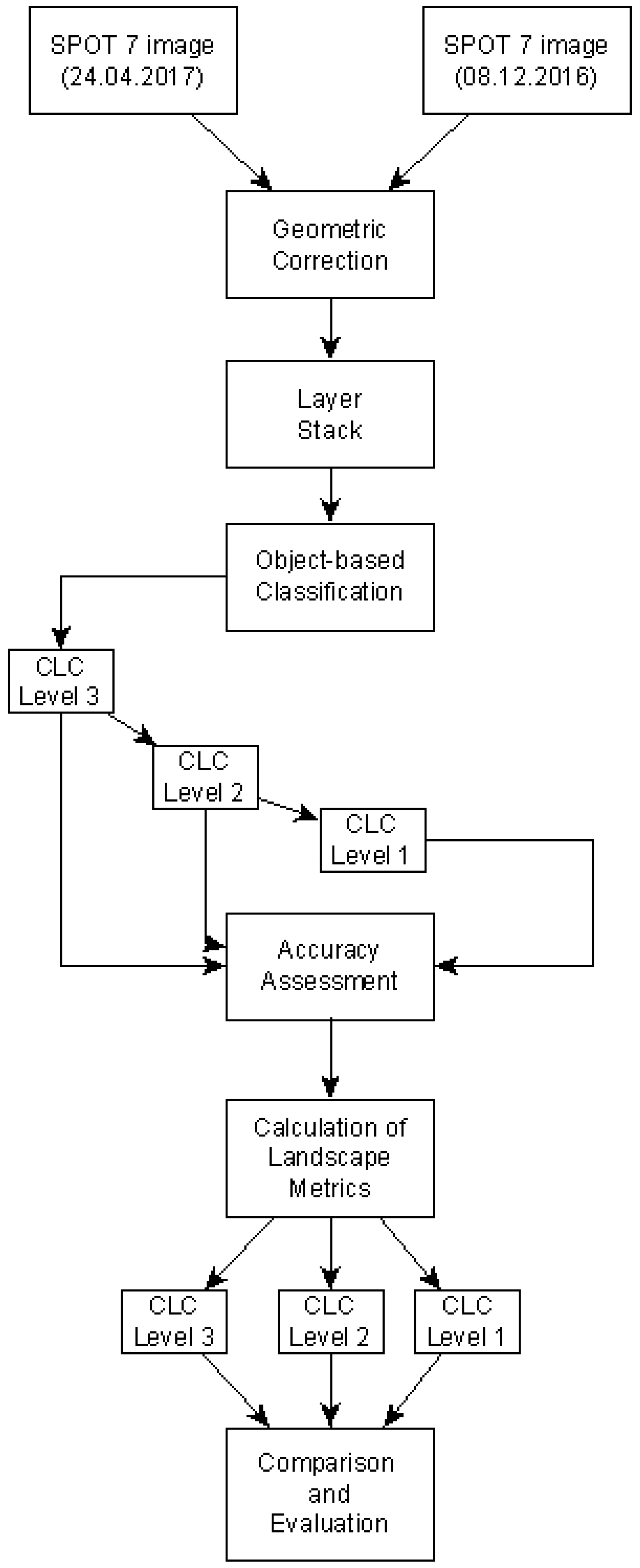
3. Methods
3.1. Pre-Processing
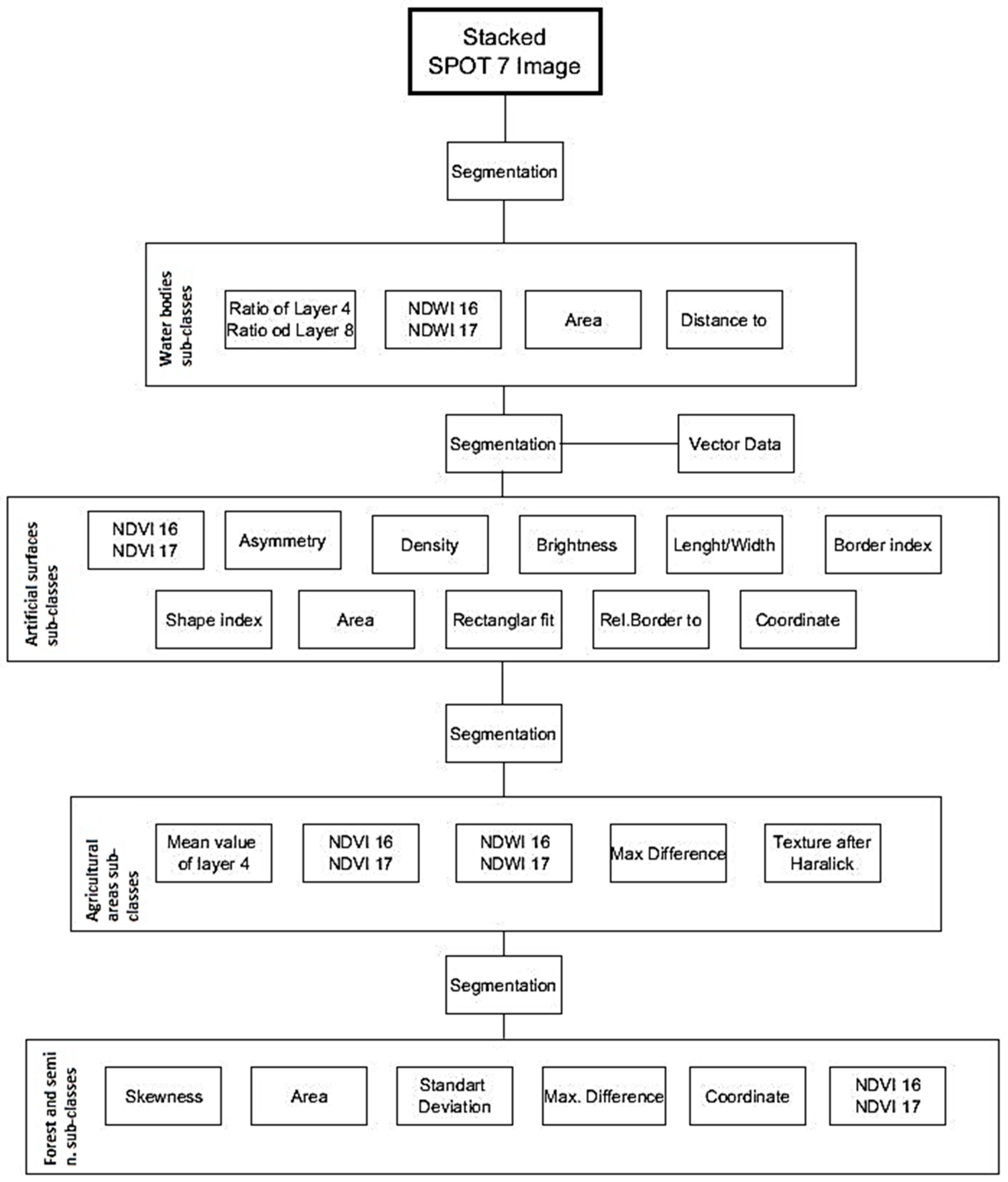
3.2. Classification
3.3. Landscape Metrics
4. Results and Discussion
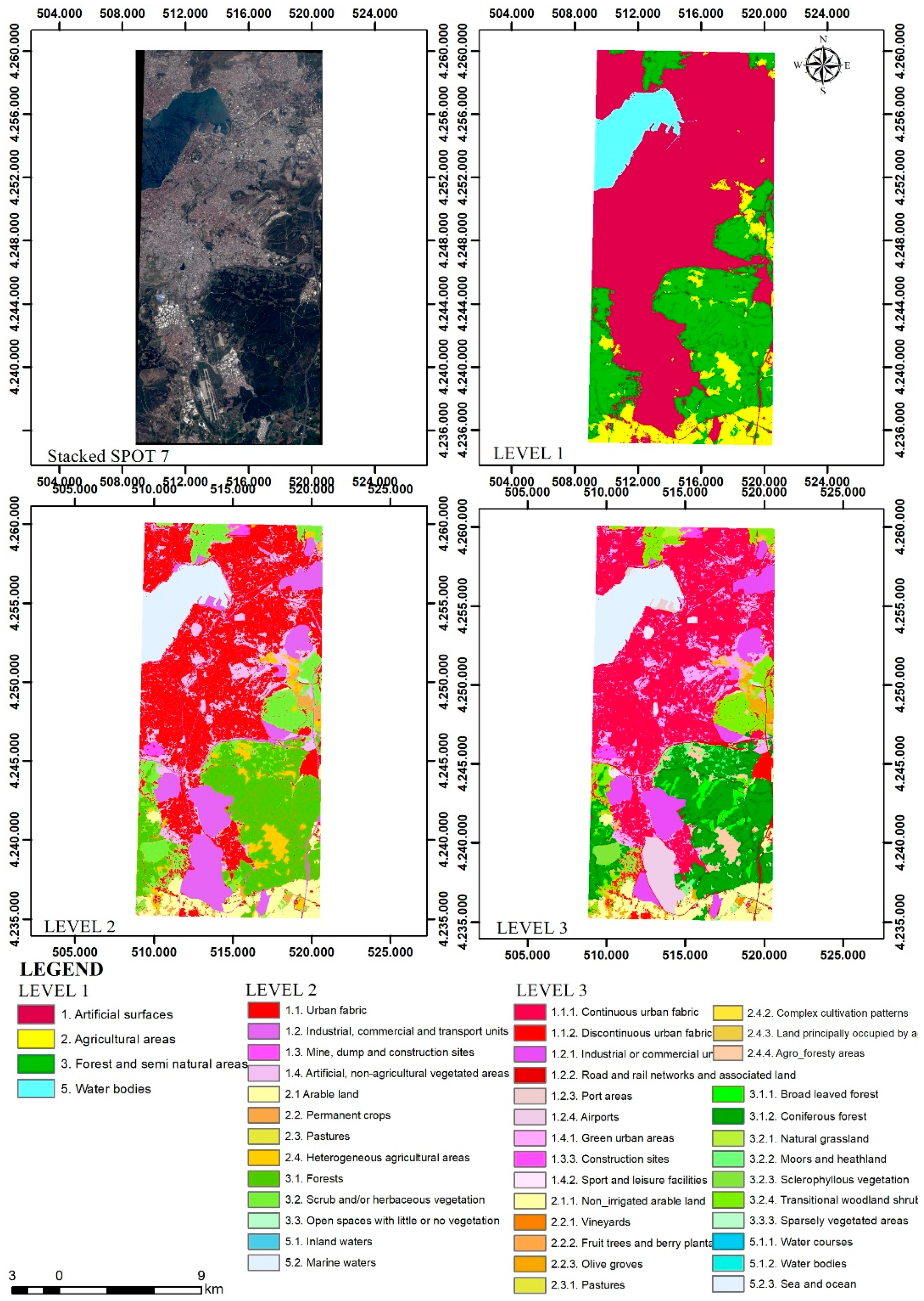
4.1. LC/LU Maps
4.2. Accuracy Assessment
4.3. Landscape Metrics
5. Conclusions
Author Contributions
Funding
Acknowledgments
Conflicts of Interest
References
- Carlson, T.N.; Arthur, S.T. The impact of land use—Land cover changes due to urbanization on surface microclimate and hydrology: A satellite perspective. Glob. Planet. Chang. 2000, 25, 49–65. [Google Scholar] [CrossRef]
- Pauleit, S.; Duhme, F. Assessing the environmental performance of land cover types for urban planning. Landsc. Urban Plan. 2000, 52, 1–20. [Google Scholar] [CrossRef]
- Pauleit, S.; Ennos, R.; Golding, Y. Modeling the environmental impacts of urban land use and land cover change—A study in Merseyside, UK. Landsc. Urban Plan. 2005, 71, 295–310. [Google Scholar] [CrossRef]
- Giri, C.P. Remote Sensing of Land Use and Land Cover Principles and Applications, 1st ed.; CRC Press: Boca Raton, FL, USA, 2012; ISBN 978-1-420-07075-0. [Google Scholar]
- Alp, G. Güncel Arazi Örtüsü/Kullanım Haritalarının Doğrudan Ve Dolaylı Yaklaşımlar Ile Üretilmesi. Master’s Thesis, Istanbul Technical University, Istanbul, Turkey, 2015. [Google Scholar]
- Topaloglu, R.H.; Sertel, E.; Musaoglu, N. Assessment of classification accuracies of Sentinel-2 and Landsat-8 data for land cover/use mapping. In Proceedings of the XXIII ISPRS Congress International Archives of the Photogrammetry, Remote Sensing & Spatial Information Sciences, Prague, Czech Republic, 12–19 July 2016. [Google Scholar]
- Goodin, D.G.; Anibas, K.L.; Bezymennyi, M. Mapping land cover and land use from object-based classification: An example from a complex agricultural landscape. Int. J. Remote Sens. 2015, 36, 4702–4723. [Google Scholar] [CrossRef]
- Vizzari, M.; Hilal, M.; Sigura, M.; Antognelli, S.; Joly, D. Urban-rural-natural gradient analysis with CORINE data: An application to the metropolitan France. Landsc. Urban Plan. 2018, 171, 18–29. [Google Scholar] [CrossRef]
- Kosztra, B.; Büttner, G.; Hazeu, G.; Arnold, S. Updated CLC Illustrated Nomenclature Guidelines. Final Report by European Environmental Agency. Available online: https://land.copernicus.eu/ (accessed on 28 March 2018).
- Brown, N.; Gerard, F.; Fuller, R. Mapping of land use classes within the CORINE land cover map of Great Britain. Cartogr. J. 2002, 39, 5–14. [Google Scholar] [CrossRef]
- Toure, S.; Stow, D.A.; Shih, H.; Weeks, J.; Lopéz-Carr, D. Land cover/land use change analysis using multi-spatial resolution data and object-based image analysis. Remote Sens. Environ. 2018, 210, 259–268. [Google Scholar] [CrossRef]
- Alganci, U.; Sertel, E.; Kaya, S. Determination of the olive trees with object based classification of Pleiades satellite image. Int. J. Environ. Geoinform. 2018, 5, 132–139. [Google Scholar] [CrossRef]
- Sertel, E.; Akay, S.S. High resolution mapping of urban areas using SPOT-5 images and ancillary data. Int. J. Environ. Geoinform. 2015, 2, 63–76. [Google Scholar] [CrossRef]
- Alganci, U.; Sertel, E.; Ozdogan, M.; Ormeci, C. Parcel-level identification of crop types using different classification algorithms and multi-resolution imagery in Southeastern Turkey. Photogramm. Eng. Remote Sens. 2013, 79, 1053–1065. [Google Scholar] [CrossRef]
- Weng, Q. Remote sensing of impervious surfaces in the urban areas: Requirements, methods, and trends. Remote Sens. Environ. 2012, 117, 34–49. [Google Scholar] [CrossRef]
- Blaschke, T. Object based image analysis for remote sensing. ISPRS J. Photogramm. Remote Sens. 2010, 65, 2–16. [Google Scholar] [CrossRef]
- Varga, O.G.; Szabó, S.; Túri, Z. Efficiency assessments of GEOBIA in land cover analysis, NE Hungary. Bull. Environ. Sci. Res. 2014, 3, 1–9. [Google Scholar]
- Myint, S.W.; Gober, P.; Brazel, A.; Grossman-Clarke, S.; Weng, Q. Per-pixel vs. object-based classification of urban land cover extraction using high spatial resolution imagery. Remote Sens. Environ. 2011, 115, 1145–1161. [Google Scholar] [CrossRef]
- Wentz, E.; Zhao, Q. Assessing validation methods for building identification and extraction. In Proceedings of the Joint Urban Remote Sensing Event (JURSE), Lausanne, Switzerland, 30 March–1 April 2015. [Google Scholar]
- Ormeci, C.; Alganci, U.; Sertel, E. Identification of crop areas Using SPOT–5 data. In Proceedings of the FIG Congress, Sydney, Australia, 11–16 April 2010. [Google Scholar]
- Blaschke, T.; Hay, G.J.; Kelly, M.; Lang, S.; Hofmann, P.; Addink, E.; Feitosa, R.Q.; van der Meer, F.; van der Werff, H.; van Coillie, F.; et al. Geographic object-based image analysis—Towards a new paradigm. ISPRS J. Photogramm. Remote Sens. 2014, 87, 180–191. [Google Scholar] [CrossRef] [PubMed]
- Lillesand, T.M.; Kiefer, R.W.; Chipman, J.W. Remote Sensing and Image Interpretation, 7th ed.; John Wiley & Sons: New York, NY, USA, 2008; ISBN 978-1-118-34328-9. [Google Scholar]
- Sertel, E.; Alganci, U. Comparison of pixel and object-based classification for burned area mapping using SPOT-6 images. Geomat. Nat. Hazards Risk 2016, 7, 1198–1206. [Google Scholar] [CrossRef]
- Zhou, W. An object-based approach for urban land cover classification: Integrating LIDAR height and intensity data. IEEE Geosci. Remote Sens. Lett. 2013, 10, 928–931. [Google Scholar] [CrossRef]
- Li, X.; Myint, S.W.; Zhang, Y.; Galletti, C.; Zhang, X.; Turner, B.L. Object-based land-cover classification for metropolitan Phoenix, Arizona, using aerial photography. Int. J. Appl. Earth Obs. Geoinf. 2014, 33, 321–330. [Google Scholar] [CrossRef]
- McGarigal, K. Landscape pattern metrics. In Encyclopedia of Environmetrics, 2nd ed.; El-Shaarawi, A.H., Piegorsch, W.W., Eds.; Wiley: Chichester, UK, 2012; Volume 6, ISBN 978-0-470-05733-9. [Google Scholar]
- Uuemaa, E.; Mander, Ü.; Marja, R. Trends in the use of landscape spatial metrics as landscape indicators: A review. Ecol. Indic. 2013, 28, 100–106. [Google Scholar] [CrossRef]
- Forman, R.; Godron, M. Landscape Ecology; John Wiley and Sons: New York, NY, USA, 1986; ISBN 0471870374. [Google Scholar]
- Forman, R.T.T. Land Mosaics: The Ecology of Landscapes and Regions, 1st ed.; Cambridge University Press: Cambridge, UK, 1995; ISBN 978-0-521-479980-6 (PB). [Google Scholar]
- Jaeger, J.A.G. Landscape division, splitting index, and effective mesh size: New measures of landscape fragmentation. Landsc. Ecol. 2000, 15, 115–130. [Google Scholar] [CrossRef]
- Turner, M.G.; Gardner, R.H.; O’Neill, R.V. Landscape Ecology in Theory and Practice: Pattern and Process; Springer: New York, NY, USA, 2001; ISBN 978-0387951225. [Google Scholar]
- Leitão, H.C.G.; Stolfi, J. A multiscale method for the reassembly of two-dimensional fragmented objects. IEEE Trans. Pattern Anal. Mach. Intell. 2002, 24, 1239–1251. [Google Scholar] [CrossRef]
- Frazier, A.E. Landscape metrics: Past progress and future directions. Curr. Landsc. Ecol. Rep. 2017, 2, 63–72. [Google Scholar] [CrossRef]
- Kedron, P.J.; Frazier, A.E.; Ovando-Montejo, G.A.; Wang, J. Surface metrics for landscape ecology: A comparison of landscape models across ecoregions and scales. Landsc. Ecol. 2018, 1–16. [Google Scholar] [CrossRef]
- McGarigal, K.; Cushman, S.A.; Neel, M.C.; Ene, E. FRAGSTATS: Spatial Pattern Analysis Program for Categorical Maps. Computer Software Program Produced by the Authors at the University of Massachusetts, Amherst, USA. 2002. Available online: http://www.umass.edu/landeco/research/fragstats/fragstats.html (accessed on 16 April 2018).
- Cushman, S.A.; McGarigal, K.; McKelvey, K.S.; Vojta, C.D.; Regan, C.M. Chapter 6. Landscape Analysis for Habitat Monitoring. In A Technical Guide for Monitoring Wildlife Habitat; U.S. Department of Agriculture, Forest Service: Washington, DC, USA, 2013. Available online: https://www.fs.usda.gov/treesearch/pubs/45223 (accessed on 24 April 2018).
- McGarigal, K.; Tagil, S.; Cushman, S.A. Surface metrics: An alternative to patch metrics for the quantification of landscape structure. Landsc. Ecol. 2009, 24, 433–450. [Google Scholar] [CrossRef]
- Plexida, S.G.; Sfougaris, A.I.; Ispikoudis, I.P.; Papanastasis, V.P. Selecting landscape metrics as indicators of spatial heterogeneity—A comparison among Greek landscapes. Int. J. Appl. Earth Obs. Geoinf. 2014, 26, 26–35. [Google Scholar] [CrossRef]
- Turkish Statistical Institute (TUIK). Available online: www.tuik.gov.tr (accessed on 2 April 2018).
- AIRBUS Defence and Space. Available online: https://www.intelligence-airbusds.com/en/147-spot-6-7-satellite-imagery (accessed on 10 April 2018).
- Definiens. Definiens© Developer 8 Reference Book; Definiens AG: Munich, Germany, 2009. [Google Scholar]
- Belgiu, M.; Drauţ, L.; Strobl, J. Quantitative evaluation of variations in rule-based classifications of land cover in urban neighborhoods using WorldView-2 imagery. ISPRS J. Photogramm. Remote Sens. 2014, 87, 205–215. [Google Scholar] [CrossRef] [PubMed]
- Hecht, R.; Kunze, C.; Hahmann, S. Measuring completeness of building footprints in OpenStreetMap over space and time. ISPRS Int. J. Geo-Inf. 2013, 2, 1066–1091. [Google Scholar] [CrossRef]
- eCognition. Trimble eCognition© Developer 9.3 for Windows Operating System Reference Book; Trimble: Germany GmbH: Munich, Germany, 2017. [Google Scholar]
- Mcfeeters, S.K. The use of the Normalized Difference Water Index (NDWI) in the delineation of open water features. Int. J. Remote Sens. 1996, 17, 1425–1432. [Google Scholar] [CrossRef]
- Turner, M.G.; O’Neill, R.V.; Gardner, R.H.; Milne, B.T. Effects of changing spatial scale on the analysis of landscape pattern. Landsc. Ecol. 1989, 3, 153–162. [Google Scholar] [CrossRef]
- Cushman, S.A.; McGarigal, K.; Neel, M.C. Parsimony in landscape metrics: Strength, universality, and consistency. Ecol. Indic. 2008, 8, 691–703. [Google Scholar] [CrossRef]
- Wu, J. Effects of changing scale on landscape pattern analysis: Scaling relations. Landsc. Ecol. 2004, 19, 125–138. [Google Scholar] [CrossRef]
- Brady, M.; Kellermann, K. Methodology for Assessing the Regional Environmental Impacts of Decoupling: A Focus on Landscape Values; SLI-Working Paper; Swedish Institute for Food and Agricultural Economics: Lund, Sweden, 2005; Volume 2. [Google Scholar]
- Tischendorf, L. Can landscape indices predict ecological processes consistently? Landsc. Ecol. 2001, 16, 235–254. [Google Scholar] [CrossRef]
- Szabó, S.; Csorba, P.; Szilassi, P. Tools for landscape ecological planning-scale, and aggregation sensitivity of the contagion type landscape metric indices. Carpathian J. Earth Environ. Sci. 2012, 7, 127–136. [Google Scholar]
- Papadimitriou, F. Modelling spatial landscape complexity using the Levenshtein Algorithm. Ecol. Inform. 2009, 4, 48–55. [Google Scholar] [CrossRef]
- McGarigal, K.; Marks, B.J. FRAGSTATS: Spatial Pattern Analysis Program for Quantifying Landscape Structure; General Technical Report; U.S. Department of Agriculture, Forest Service, Pacific Northwest Research Station: Portland, OR, USA, 1995.
- Dramstad, W.E. Spatial metrics—Useful indicators for society or mainly fun tools for landscape ecologists? Norsk Geografisk Tidsskrift 2009, 63, 246–254. [Google Scholar] [CrossRef]


| Layers | SPOT 7 Image Bands |
|---|---|
| Layer 1 | Red band of 2017 |
| Layer 2 | Green band of 2017 |
| Layer 3 | Blue band of 2017 |
| Layer 4 | Near-Infrared band of 2017 |
| Layer 5 | Red band of 2016 |
| Layer 6 | Green band of 2016 |
| Layer 7 | Blue band of 2016 |
| Layer 8 | Near-Infrared band of 2016 |
| Class Name | Scale | Shape | Compactness |
|---|---|---|---|
| Sea and Ocean | 1500 | 0.6 | 0.6 |
| Water Bodies | 500 | 0.6 | 0.5 |
| Water Courses | 85 | 0.7 | 0.8 |
| Artificial Surfaces sub-classes | 250, 85, 200 | 0.9, 0.8, 0.3 | 0.5, 0.6, 0.5 |
| Agricultural Areas sub-classes | 100, 85 | 0.7, 0.5 | 0.5, 0.5 |
| Forest and Semi-natural Areas sub-classes | 1000, 500, 100 | 0.3, 0.4, 0.6 | 0.6, 0.6, 0.5 |
| Thematic Layer | Purpose |
|---|---|
| OpenStreetMap Road Data | Segmentation/Classification of Road and rail networks and associated land |
| Wikimapia Open Source Data | Segmentation/Classification of all Agricultural Areas sub-classes (in Level-3) |
| Features/Indices | Explanations |
|---|---|
| NDVI 2017 | Normalized difference vegetation index; NDVI = (Layer 4 − Layer 1)/(Layer 4 + Layer 1) |
| NDVI2016 | Normalized difference vegetation index; NDVI = (Layer 8 − Layer 5)/(Layer 8 + Layer 5) |
| NDWI2017 | Normalized difference water index; NDWI = (Layer 2 − Layer 4)/(Layer 2 + Layer 4) |
| NDWI2016 | Normalized difference water index; NDWI = (Layer 6 − Layer 8)/(Layer 6 + Layer 8) |
| Ratio of layer 4 | The amount that Layer 4 contributes to the total brightness |
| Ratio of layer 8 | The amount that Layer 8 contributes to the total brightness |
| Mean value of layer 4 | Mean intensity values in the NIR 2017 band |
| Mean value of layer 8 | Mean intensity values in the NIR 2016 band |
| Brightness | Mean of the brightness values in an image |
| Maximum difference | Calculates the mean difference between the feature value of an image object and its neighbors of a selected class |
| Standard deviation of layer 4 | The standard deviation of the NIR 2017 band derived from intensity values of all pixels in this channel |
| Skewness of layer 4 | The distribution of layer 4 intensity values of all pixels that form an image object |
| Shape index | Measure of overall shape complexity |
| Border index | Describes how jagged an image object is; the more jagged, the higher its border index |
| Asymmetry | Compares an image object with an approximated ellipse around the given image object |
| Rectangular fit | Describes how well an image object fits into a rectangle of similar size and proportions |
| Density | The distribution in space of the pixels of an image object |
| Area | The total number of pixels in the object |
| Length/Width | The length-to-width ratio of the main line of an object |
| Coordinate (X, Y Center) | X-position and Y-position of the center of an image object. The calculation is based on the center of gravity (geometric center) of the image object in the internal map. |
| Related border to | Determines the relative border length an object shares with neighbor objects of a certain class |
| Distance to | The distance (in pixels) of the image object’s center concerned to the closest image object’s center assigned to a defined class |
| Texture after Haralick | Texture features are used to evaluate the texture of image objects. Texture after Haralick features are calculated from gray level co-occurrence matrix. |
| Metric | Description |
|---|---|
| Percentage of Landscape (PLAND) | The percentage of the landscape comprised of a particular patch type |
| Number of Patches (NP) | Number of patches of corresponding patch type (class) |
| Patch Density (PD) | Number of patches of corresponding patch type (class) per unit area |
| Largest Patch Index (LPI) | The area (m2) of the largest patch in the landscape divided by total landscape area (m2) |
| Total Edge (TE) | The sum of the lengths (m) of all edge segments in the landscape |
| Edge Density (ED) | The sum of the lengths (m) of all edge segments in the landscape, divided by the total landscape area (m2) |
| Landscape Shape Index (LSI) | A standardized measure of patch compactness that adjusts for the size of the patch |
| Area-Weighted Mean Shape Index (SHAPE_AM) | Weighting patches according to their size, on contrary to LSI in which the total length of edge is compared to a landscape with a standard shape (square) of the same size and without any internal edge |
| Total Core Area (TCA) | The sum of the core areas of each patch (m2) |
| Euclidean Nearest Neighbor Distance Area-Weighted Mean (ENN_AM) | Shortest straight-line distance (m) between a focal patch and its nearest neighbor of the same class |
| Splitting Index (SPLIT) | The number of patches obtained with subdividing the landscape into equal-sized patches based on the effective mesh size |
| Aggregation Index (AI) | The ratio of the observed number of like adjacencies to the maximum possible number of like adjacencies given the proportion of the landscape comprised of each patch type, given as a percentage |
| Class Code | Class Name | Producer’s Accuracy (%) | User’s Accuracy (%) |
|---|---|---|---|
| 1.1.1 | Continuous urban fabric | 91.67 | 100.00 |
| 1.1.2 | Discontinuous urban fabric | 87.50 | 100.00 |
| 1.2.1 | Industrial or commercial units | 90.00 | 81.82 |
| 1.2.2 | Road and rail networks and associated land | 90.00 | 90.00 |
| 1.2.3 | Port areas | 100.00 | 100.00 |
| 1.2.4 | Airports | 100.00 | 100.00 |
| 1.3.3 | Construction sites | 60.00 | 75.00 |
| 1.4.1 | Green urban areas | 77.78 | 77.78 |
| 1.4.2 | Sport and leisure facilities | 100.00 | 100.00 |
| 2.1.1 | Non-irrigated arable land | 77.78 | 63.64 |
| 2.2.1 | Vineyards | 100.00 | 71.43 |
| 2.2.2 | Fruit trees and berry plantations | 50.00 | 100.00 |
| 2.2.3 | Olive groves | 100.00 | 88.89 |
| 2.4.2 | Complex cultivation patterns | 80.00 | 57.14 |
| 2.4.3 | Land principally occupied by agriculture | 62.50 | 100.00 |
| 2.4.4 | Agro-forestry areas | 77.78 | 87.50 |
| 3.1.1 | Broad-leaved forest | 100.00 | 75.00 |
| 3.1.2 | Coniferous forest | 73.33 | 84.62 |
| 3.2.1 | Natural grassland | 100.00 | 50.00 |
| 3.2.2 | Moors and heathland | 66.67 | 100.00 |
| 3.2.3 | Sclerophyllous vegetation | 77.78 | 87.50 |
| 3.2.4 | Transitional woodland shrub | 77.78 | 87.50 |
| 5.1.1 | Water courses | 100.00 | 100.00 |
| 5.1.2 | Water bodies | 100.00 | 100.00 |
| 5.2.3 | Sea and ocean | 100.00 | 100.00 |
| Class Code | Class Name | Producer’s Accuracy (%) | User’s Accuracy (%) |
|---|---|---|---|
| 1.1 | Urban fabric | 90.63 | 100.00 |
| 1.2 | Industrial, commercial and transport units | 96.67 | 90.63 |
| 1.3 | Mine, dump and construction sites | 60.00 | 75.00 |
| 1.4 | Artificial, non-agricultural vegetated areas | 85.71 | 85.71 |
| 2.1 | Arable land | 80.00 | 80.00 |
| 2.2 | Permanent crops | 82.35 | 93.33 |
| 2.4 | Heterogeneous agricultural areas | 77.27 | 77.27 |
| 3.1 | Forests | 95.83 | 92.00 |
| 3.2 | Shrub and/or herbaceous vegetation associations | 86.21 | 80.65 |
| 5.1 | Inland waters | 100.00 | 100.00 |
| 5.2 | Marine waters | 100.00 | 100.00 |
| Class Code | Class Name | Producer’s Accuracy (%) | User’s Accuracy (%) |
|---|---|---|---|
| 1 | Artificial surfaces | 95.06 | 98.72 |
| 2 | Agricultural areas | 91.67 | 89.80 |
| 3 | Forest and semi-natural areas | 90.57 | 87.27 |
| 5 | Water bodies | 100.00 | 100.00 |
| Class Code | Class Name | Landscape Metrics | |||||||||||
|---|---|---|---|---|---|---|---|---|---|---|---|---|---|
| PLAND | NP | PD | LPI | TE | ED | LSI | SHAPE_AM | TCA | ENN_AM | SPLIT | AI | ||
| 1.1.1 | Continuous urban fabric | 32.20 | 25,183.00 | 84.95 | 0.27 | 9,054,195.00 | 305.44 | 231.70 | 2.25 | 195.75 | 3.60 | 27,522.07 | 96.46 |
| 1.1.2 | Discontinuous urban fabric | 1.28 | 640.00 | 2.16 | 0.50 | 326,466.00 | 11.01 | 41.95 | 2.98 | 121.82 | 28.81 | 39,296.07 | 96.84 |
| 1.2.1 | Industrial or commercial units | 6.27 | 51.00 | 0.17 | 1.94 | 84,885.00 | 2.86 | 4.92 | 1.53 | 1561.90 | 723.14 | 1471.41 | 99.86 |
| 1.2.2 | Road and rail networks and associated land | 4.69 | 1358.00 | 4.58 | 3.95 | 8,950,512.00 | 301.94 | 600.10 | 515.82 | 21.32 | 6.23 | 638.43 | 75.89 |
| 1.2.3 | Port areas | 0.29 | 3.00 | 0.01 | 0.23 | 15,060.00 | 0.51 | 4.04 | 2.81 | 41.79 | 1991.98 | 178,093.85 | 99.51 |
| 1.2.4 | Airports | 2.56 | 1.00 | 0.00 | 2.56 | 17,238.00 | 0.58 | 1.56 | 1.56 | 691.38 | - | 1528.61 | 99.97 |
| 1.3.3 | Construction sites | 8.19 | 1623.00 | 5.48 | 0.30 | 1,909,116.00 | 64.40 | 96.88 | 3.83 | 278.50 | 15.23 | 21,613.86 | 97.08 |
| 1.4.1 | Green urban areas | 0.54 | 8.00 | 0.03 | 0.29 | 35,193.00 | 1.19 | 6.93 | 4.70 | 81.95 | 7362.11 | 67,896.71 | 99.30 |
| 1.4.2 | Sport and leisure facilities | 0.43 | 4.00 | 0.01 | 0.15 | 11,457.00 | 0.39 | 2.54 | 1.29 | 84.79 | 3020.44 | 201,152.89 | 99.80 |
| 2.1.1 | Non-irrigated arable land | 4.79 | 138.00 | 0.47 | 1.28 | 288,921.00 | 9.75 | 19.17 | 5.17 | 748.22 | 64.93 | 3563.10 | 99.28 |
| 2.2.1 | Vineyards | 0.10 | 15.00 | 0.05 | 0.05 | 12,297.00 | 0.41 | 5.59 | 2.10 | 7.52 | 332.31 | 3,414,936.14 | 98.74 |
| 2.2.2 | Fruit trees and berry plantations | 0.12 | 35.00 | 0.12 | 0.02 | 21,129.00 | 0.71 | 8.88 | 2.58 | 1.95 | 1171.44 | 6,866,804.18 | 98.01 |
| 2.2.3 | Olive groves | 1.01 | 50.00 | 0.17 | 0.29 | 125,280.00 | 4.23 | 18.11 | 4.08 | 58.96 | 242.77 | 86,627.64 | 98.51 |
| 2.3.1 | Pastures | 0.01 | 10.00 | 0.03 | 0.00 | 2112.00 | 0.07 | 3.16 | 1.47 | 0.00 | 50.80 | 345,408,656.43 | 98.04 |
| 2.4.2 | Complex cultivation patterns | 0.13 | 11.00 | 0.04 | 0.04 | 20,487.00 | 0.69 | 8.31 | 2.91 | 5.78 | 2971.33 | 3,923,394.11 | 98.21 |
| 2.4.3 | Land principally occupied by agriculture | 0.74 | 56.00 | 0.19 | 0.10 | 90,822.00 | 3.06 | 15.29 | 3.60 | 41.37 | 760.56 | 250,602.11 | 98.55 |
| 2.4.4 | Agro-forestry areas | 1.76 | 58.00 | 0.20 | 0.69 | 142,941.00 | 4.82 | 15.64 | 3.64 | 241.81 | 126.58 | 17,331.17 | 99.04 |
| 3.1.1 | Broad-leaved forest | 1.26 | 33.00 | 0.11 | 0.17 | 98,382.00 | 3.32 | 12.72 | 2.59 | 142.88 | 73.85 | 111,850.51 | 99.09 |
| 3.1.2 | Coniferous forest | 14.44 | 181.00 | 0.61 | 3.56 | 888,384.00 | 29.97 | 33.94 | 6.47 | 2122.29 | 5.92 | 529.59 | 99.24 |
| 3.2.1 | Natural grassland | 0.27 | 1.00 | 0.00 | 0.27 | 13,779.00 | 0.46 | 3.88 | 3.88 | 47.14 | - | 141,527.10 | 99.51 |
| 3.2.2 | Moors and heathland | 1.65 | 523.00 | 1.76 | 0.12 | 411,735.00 | 13.89 | 46.48 | 4.57 | 52.44 | 18.37 | 157,027.38 | 96.92 |
| 3.2.3 | Sclerophyllous vegetation | 1.23 | 160.00 | 0.54 | 0.68 | 143,505.00 | 4.84 | 18.79 | 3.41 | 174.44 | 3.24 | 21,037.03 | 98.60 |
| 3.2.4 | Transitional woodland shrub | 6.00 | 628.00 | 2.12 | 0.71 | 583,698.00 | 19.69 | 34.58 | 4.04 | 749.56 | 16.17 | 5439.46 | 98.81 |
| 3.3.3 | Sparsely vegetated areas | 0.10 | 15.00 | 0.05 | 0.06 | 20,730.00 | 0.70 | 9.36 | 2.67 | 8.32 | 269.26 | 2,485,926.97 | 97.73 |
| 5.1.1 | Water courses | 0.03 | 16.00 | 0.05 | 0.01 | 12,402.00 | 0.42 | 10.47 | 3.15 | 0.00 | 18.58 | 113,407,894.57 | 95.17 |
| 5.1.2 | Water bodies | 0.01 | 2.00 | 0.01 | 0.01 | 1545.00 | 0.05 | 2.15 | 1.59 | 0.00 | 21,949.51 | 134,859,989.85 | 99.03 |
| 5.2.3 | Sea and ocean | 6.12 | 1.00 | 0.00 | 6.12 | 42,405.00 | 1.43 | 2.49 | 2.49 | 1665.32 | - | 266.93 | 99.95 |
| Class Code | Class Name | Landscape Metrics | |||||||||||
|---|---|---|---|---|---|---|---|---|---|---|---|---|---|
| PLAND | NP | PD | LPI | TE | ED | LSI | SHAPE_AM | TCA | ENN_AM | SPLIT | AI | ||
| 1.1 | Urban fabric | 33.47 | 25,809.00 | 87.07 | 0.50 | 9,378,078.00 | 316.37 | 235.36 | 2.28 | 317.63 | 3.65 | 16,106.63 | 96.47 |
| 1.2 | Industrial, commercial and transport units | 13.82 | 1189.00 | 4.01 | 13.14 | 9,011,094.00 | 303.99 | 352.03 | 324.49 | 2372.95 | 3.83 | 57.91 | 91.77 |
| 1.3 | Mine, dump and construction sites | 0.54 | 8.00 | 0.03 | 0.29 | 35,193.00 | 1.19 | 6.93 | 4.70 | 81.95 | 7362.11 | 67,896.71 | 99.30 |
| 1.4 | Artificial, non-agricultural vegetated areas | 8.62 | 1621.00 | 5.47 | 0.30 | 1,917,036.00 | 64.67 | 94.83 | 3.73 | 364.24 | 16.25 | 19,268.59 | 97.21 |
| 2.1 | Arable land | 4.79 | 138.00 | 0.47 | 1.28 | 288,921.00 | 9.75 | 19.17 | 5.17 | 748.22 | 64.93 | 3563.10 | 99.28 |
| 2.2 | Permanent crops | 1.23 | 82.00 | 0.28 | 0.29 | 153,711.00 | 5.19 | 20.12 | 3.98 | 72.96 | 172.43 | 79,004.61 | 98.50 |
| 2.3 | Pastures | 0.01 | 10.00 | 0.03 | 0.00 | 2112.00 | 0.07 | 3.16 | 1.47 | 0.00 | 50.80 | 345,408,656.43 | 98.04 |
| 2.4 | Heterogeneous agricultural areas | 2.63 | 119.00 | 0.40 | 0.69 | 247,434.00 | 8.35 | 22.14 | 3.64 | 294.39 | 128.78 | 15,882.30 | 98.86 |
| 3.1 | Forests | 15.70 | 178.00 | 0.60 | 4.79 | 864,522.00 | 29.16 | 31.68 | 6.63 | 2397.37 | 5.66 | 341.21 | 99.33 |
| 3.2 | Shrub and/or herbaceous vegetation associations | 9.15 | 1297.00 | 4.38 | 0.93 | 1,133,607.00 | 38.24 | 54.40 | 4.11 | 1041.76 | 14.41 | 3547.41 | 98.46 |
| 3.3 | Open spaces with little or no vegetation | 0.10 | 15.00 | 0.05 | 0.06 | 20,730.00 | 0.70 | 9.36 | 2.67 | 8.32 | 269.26 | 2,485,926.97 | 97.73 |
| 5.1 | Inland waters | 0.04 | 18.00 | 0.06 | 0.01 | 13,947.00 | 0.47 | 10.06 | 2.73 | 0.00 | 3622.90 | 61,603,568.04 | 96.05 |
| 5.2 | Marine waters | 6.12 | 1.00 | 0.00 | 6.12 | 42,405.00 | 1.43 | 2.49 | 2.49 | 1665.32 | - | 266.93 | 99.95 |
| Class Code | Class Name | Landscape Metrics | |||||||||||
|---|---|---|---|---|---|---|---|---|---|---|---|---|---|
| PLAND | NP | PD | LPI | TE | ED | LSI | SHAPE_AM | TCA | ENN_AM | SPLIT | AI | ||
| 1 | Artificial surfaces | 56.45 | 953.00 | 3.21 | 55.43 | 1,517,148.00 | 51.18 | 29.33 | 19.89 | 15,050.68 | 3.31 | 3.26 | 99.67 |
| 2 | Agricultural areas | 8.66 | 138.00 | 0.47 | 1.39 | 537,900.00 | 18.15 | 26.54 | 4.87 | 1310.37 | 42.66 | 1960.96 | 99.24 |
| 3 | Forest and seminatural areas | 24.96 | 1148.00 | 3.87 | 6.68 | 1,422,033.00 | 47.97 | 41.33 | 6.20 | 4039.79 | 6.53 | 177.95 | 99.30 |
| 5 | Water bodies | 6.16 | 18.00 | 0.06 | 6.13 | 55,929.00 | 1.89 | 3.27 | 2.58 | 1665.32 | 24.96 | 266.54 | 99.92 |
© 2018 by the authors. Licensee MDPI, Basel, Switzerland. This article is an open access article distributed under the terms and conditions of the Creative Commons Attribution (CC BY) license (http://creativecommons.org/licenses/by/4.0/).
Share and Cite
Sertel, E.; Topaloğlu, R.H.; Şallı, B.; Yay Algan, I.; Aksu, G.A. Comparison of Landscape Metrics for Three Different Level Land Cover/Land Use Maps. ISPRS Int. J. Geo-Inf. 2018, 7, 408. https://doi.org/10.3390/ijgi7100408
Sertel E, Topaloğlu RH, Şallı B, Yay Algan I, Aksu GA. Comparison of Landscape Metrics for Three Different Level Land Cover/Land Use Maps. ISPRS International Journal of Geo-Information. 2018; 7(10):408. https://doi.org/10.3390/ijgi7100408
Chicago/Turabian StyleSertel, Elif, Raziye Hale Topaloğlu, Betül Şallı, Irmak Yay Algan, and Gül Aslı Aksu. 2018. "Comparison of Landscape Metrics for Three Different Level Land Cover/Land Use Maps" ISPRS International Journal of Geo-Information 7, no. 10: 408. https://doi.org/10.3390/ijgi7100408
APA StyleSertel, E., Topaloğlu, R. H., Şallı, B., Yay Algan, I., & Aksu, G. A. (2018). Comparison of Landscape Metrics for Three Different Level Land Cover/Land Use Maps. ISPRS International Journal of Geo-Information, 7(10), 408. https://doi.org/10.3390/ijgi7100408