Regional Landslide Identification Based on Susceptibility Analysis and Change Detection

Abstract

Landslide identification is an increasingly important research topic in remote sensing and the study of natural hazards. It is essential for hazard prevention, mitigation, and vulnerability assessments. Despite great efforts over the past few years, its accuracy and efficiency can be further improved. Thus, this study combines the two most popular approaches: susceptibility analysis and change detection thresholding, to derive a landslide identification method employing novel identification criteria. Through a quantitative evaluation of the proposed method and masked change detection thresholding method, the proposed method exhibits improved accuracy to some extent. Our susceptibility-based change detection thresholding method has the following benefits: (1) it is a semi-automatic landslide identification method that effectively integrates a pixel-based approach with an object-oriented image analysis approach to achieve more precise landslide identification; (2) integration of the change detection result with the susceptibility analysis result represents a novel approach in the landslide identification research field.

1. Introduction

Large landslides are a global phenomenon causing damage and loss of life [1]. As a result, landslide research has become a hot research topic in which landslide identification receives particular attention. Currently, there are numerous approaches to landslide identification, with visual interpretation and field surveys being the most traditional and widely used approaches for the elaboration of inventory maps by scientists and administrative bodies [2]. However, visual interpretation and field surveys have fatal shortcomings. First, they both require extensive labor or monetary investment. Second, detailed field surveys, which are time-intensive and difficult to conduct in rugged and forest terrain, often incorporate miscalculations [3]. In recent years, with the development of remote sensing (RS), geographical information systems (GIS), image processing technology, and the availability of very high resolution (VHR) remote-sensing images (i.e., spaceborne, airborne, and terrestrial), landslides can be mapped more accurately, completely, and rapidly than ever before [4,5]. Because of this, the accuracy of landslide automatic/semi-automatic identification still has plenty of room for improvement; when its accuracy matches that of traditional visual interpretation and field surveys, it can completely replace the latter. Therefore, researching landslide automatic/semi-automatic identification methods can compensate for the shortcomings of traditional approaches. In addition, regional landslide automatic/semi-automatic identification research will help governments and relevant institutions develop effective disaster prevention and mitigation policies under reduced investment conditions; for example, maps illustrating the level of damage to affected buildings could prevent construction in historically landslide-prone areas [6].

In current landslide identification research, popular approaches involve object-oriented image analysis and pixel-based approaches. Image objects are the basic processing unit of the first approach, which use a specific method to process RS or high-resolution (HR) images and segment several similar spectral signature pixels in one object before conducting landslide detection or inventory mapping. For example, Dou [7] used an integrated approach comprising object-oriented image analysis (OOIA), a genetic algorithm (GA), and a case-based reasoning (CBR) technique to conduct image segmentation and feature optimization for landslide detection. Huang [8] used object-oriented change detection (OOCD) combined with HR images to classify land cover and detect landslides. OOIA has also been used to detect landslides in the Baichi catchment in northern Taiwan [9]. Martha [10] used segment optimization to enhance the accuracy of landslide boundary detection. This type of method can easily conduct land cover classification, then detect landslides using the classification results. However, due to a lack of background information, identifying landslides from the detected objects can be problematic.

Thus, some studies have replaced RS and HR images with a susceptibility map to conduct landslide detection and inventory mapping [11,12,13,14]. Mondini [15] combined change detection results with a classification model and achieved excellent results. However, whilst susceptibility-based OOIA is more robust, it faces the problem of over-detection or mapping. Therefore, in susceptibility-based landslide detection or mapping research, a reliable result is required to help to improve accuracy. Many researchers use different approaches to achieve reliable results. Broeckx [16] mapped landslides visually from Google Earth data and conducted a susceptibility assessment. Merghadi [17] performed a landslide susceptibility assessment using several machine learning methods to generate a landslide prone area. Meanwhile, several studies have also used the machine learning approach to calculate susceptibility and all received good results [18,19,20]. Other research has used DEM (Digital Elevation Model) or terrain models to analyze surface geomorphological features and landslide-induced changes because they provide more detailed geomorphological features [21,22,23].

In the second approach, the pixel-based approach, single pixels are the basic processing element. The most common method is change detection (CD) due to its simplicity and applicability [24,25]. Chen [26] combined the deep convolution neural network (DCNN) with spatial temporal context learning (STCL) to identify landslide areas. Raspini [27] monitored ground deformation by comparing multi-temporal images based on a pixel unit. Danneels [28] using the maximum likelihood ratio (MLR) and an artificial neural network (ANN) classification to identify landslides on a the pixel scale. Travelletti [29] used an image correlation technique to conduct landslide identification. However, whilst pixel-based approaches can reveal changed region, they cannot identify the type of change that has occurred in the region.

By combining these two popular approaches, their dual benefits can outweigh their respective shortcomings. Thus, this study builds on previous research to provide an approach to regional landslide semi-automatic identification called the susceptibility-based change detection thresholding (SCDT) method. The SCDT method contains the following steps: (1) employ the change detection threshold (CDT) method to obtain change regions, the CDT method can provide three types of candidate regions where changes have occurred (such as land cover changes or landslide-induced changes): landslide candidate regions, uncertain regions, and non-landslide regions. In this study, we regard the CDT result as the number of objects that are assigned to each type of region; (2) calculate the landslide susceptibility of the study area, the fundamental axiom of susceptibility assessments is “the past and present are keys to the future” (i.e., areas where landslides have occurred in the past will most likely be affected by landslides in the future). Moreover, areas with environmental conditions similar to those areas that have already been affected by landslides are more prone to landslides [30,31]. Landslide susceptibility analysis (LSA) is the most significant step in landslide risk assessments [32] as it can reflect landslide-prone areas or the possibility of landslide occurrence in a study area using abundant background information. Thus, it is possible that the LSA results can help identify the result of CDT and improve the landslide identification accuracy; (3) integrate the two results to identify whether the objects belong to actual landslides, which is a difference between this study and other studies; the two results are simply overlaid to manually identify landslides.

2. Materials and Methods

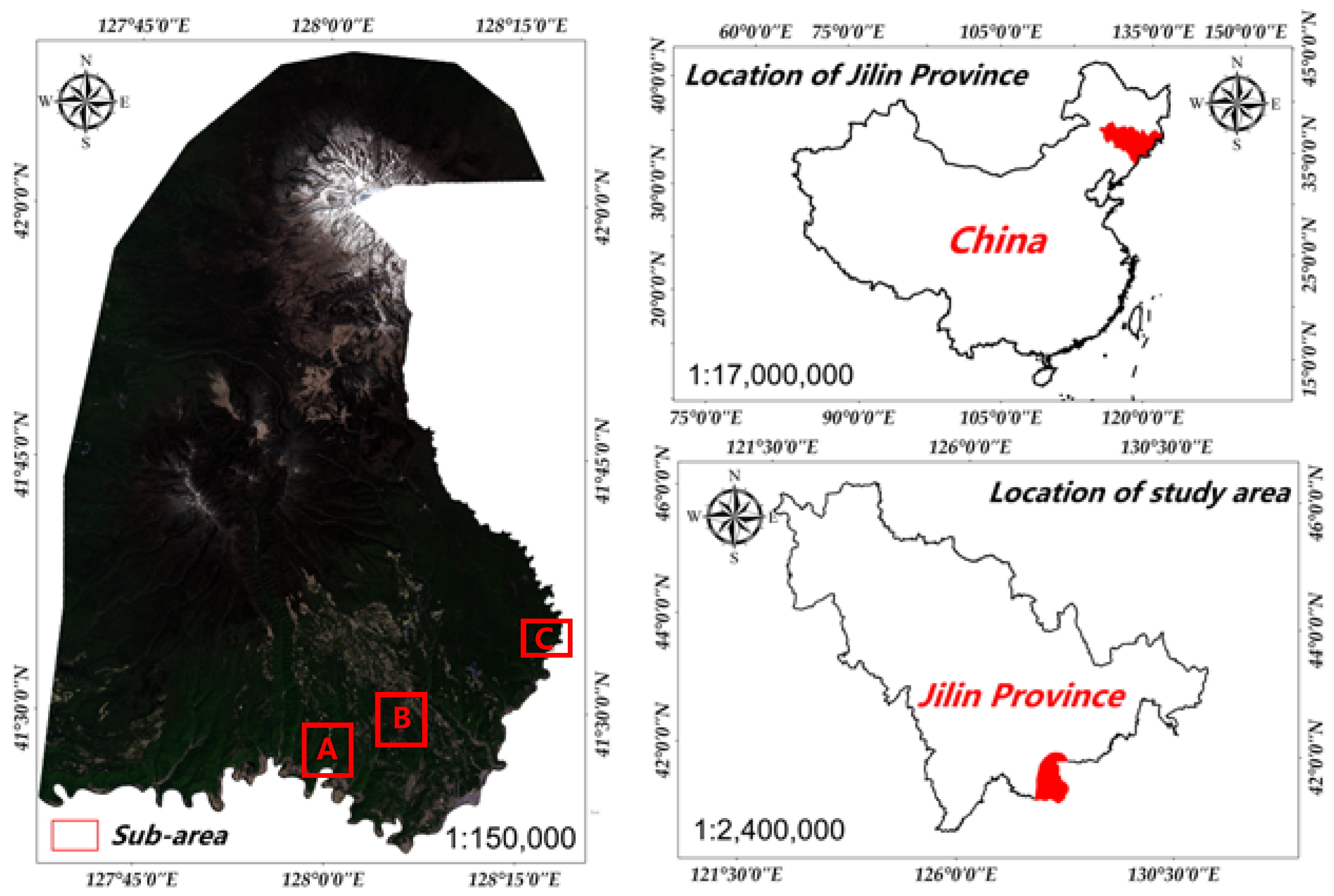
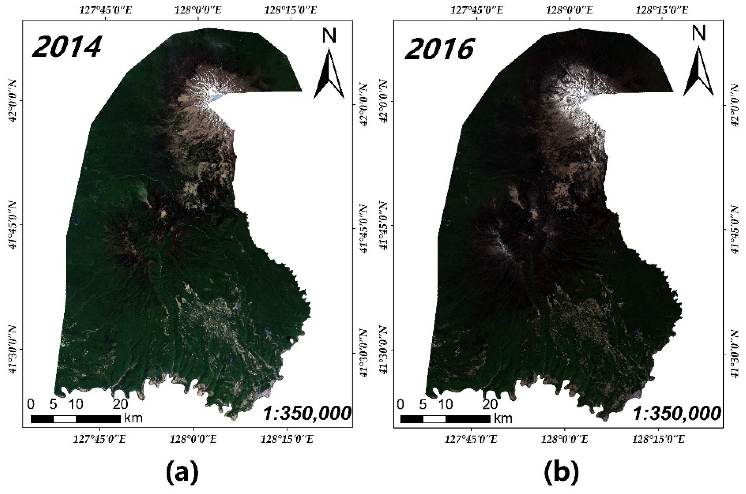
2.1. Study Area and Datasets

The study area is located south-east of Jilin Province in China with a total area of approximatively 3200 km² (Figure 1). The eastern and southern regions of the study area border North Korea. The topography and geomorphology of the entire study area is extremely complex, and there are many large mountains and canyons distributed across it. The elevations range from 2669 m to 600 m; slopes range from 75° to 15°, and many regions have slopes higher than 35°. As a result, some regions exhibit topography and geomorphology that is conducive to landslides. Annual rainfall ranges from 700 to 1400 mm and precipitation from June to September accounts for 60–70% of the annual precipitation; this often causes extreme rainfall events and provides an external incentive for landslides. In addition, Changbai Mountain, one of the most famous mountains in eastern Asia, is a dormant volcano.

In terms of the dataset, we utilized May 2014 and May 2016 Landsat 8 OLI (Operational Land Imager) images as the pre- and post-event images of the landslide area. The Landsat 8 OLI includes nine bands; the spatial resolution of eight bands are 30 m, plus a panchromatic band with a spatial resolution of 15 m. All nine bands are combined with different RGB schemes for the interpretation of different ground objects. Compared to historical Landsat TM images, Landsat 8 has added two new bands. Among them, the panchromatic band eight has exhibited better performance distinguishing vegetation and non-vegetation features. The nine bands of Landsat 8 data are more appropriate for the CD method because they can more comprehensively detect change areas. The landslide inventory was provided by the Jilin Institute of Geological Environment Monitoring (JIGEM). The landslide inventory documents the exact location and boundary and other relevant information of the landslides that occurred between the years of 2000 and 2016 (Figure 2). According to the inventory, rotational and planar shallow landslides are the most common landslide types that occurred in Jilin province, and scarcely any deep-seated landslides and landfalls were document in the inventory. A total of 141 rotational and planar shallow landslides occurred during this period, the largest rotational landslide area covered almost 29,000 m², and the smallest shallow planar landslide was just 95 m². Between 2014 and 2016 there were 10 rotational and planar shallow landslides that occurred in study area. Based on variations in land cover, geological and topographical/geomorphological conditions represent the background information for landslides. Susceptibility results was used to express the comprehensive background information according to the experience of former studies [33]. Meanwhile, 12 parameters were selected to calculate the susceptibility of the study area on the basis of relevant research [34,35]. Nine of the parameters were extracted from a 1:50,000 topographic map from 2004 to indicate the pre-landslide topographic and geomorphologic conditions for the study area (i.e., slope gradient, altitude, slope aspect, curvature, plane-curvature, profile-curvature, terrain roughness index (TRI), degree of relief index (DRI), slope length and gradient slope index (LSI)). To express geological conditions, 1:50,000 lithological and geological structure data were used; the land-use/land-cover (LULC) data was used to indicate the human disturbance of the study area, and all data mentioned above were also provide by JIGEM.

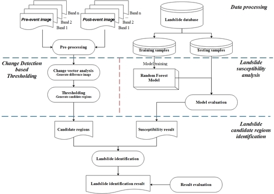
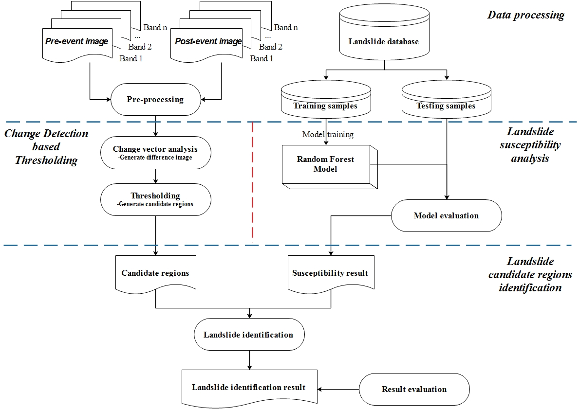
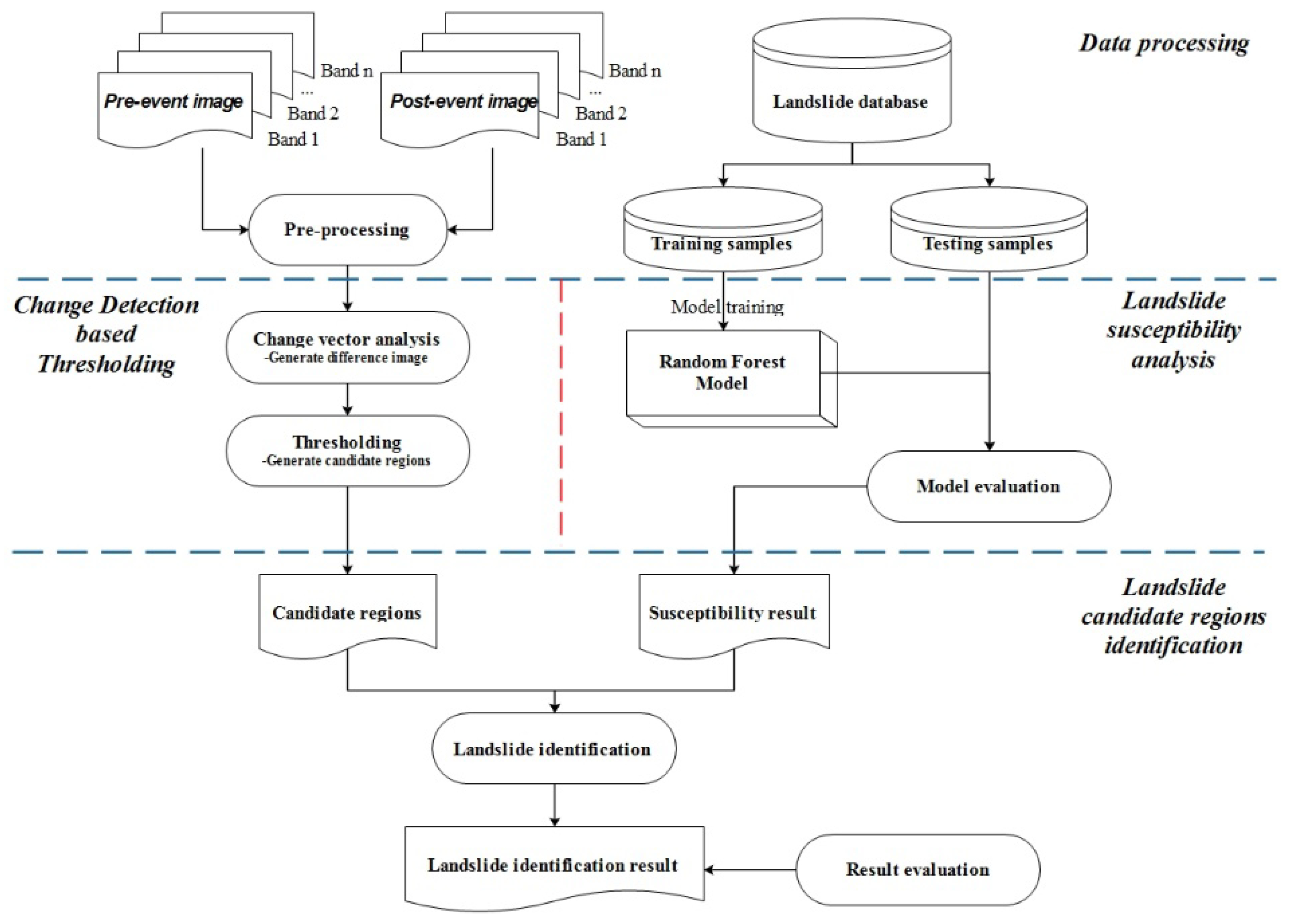
2.2. Methodology

Our proposed SCDT method comprises two main parts: CDT and LSA. In the data processing step, we conducted pre-processing so that the pre- and post-event images appeared to have been acquired under similar atmospheric and illumination conditions. Landsat 8 OLI data were used to conduct the regional landslide semi-automatic identification in this study. After the first step, CDT was conducted using processed images, a difference image (DI) was generated using change vector analysis (CVA), several tests were performed to determine the threshold, then these thresholds were used to generate the candidate regions. In the LSA step, the aforementioned data, provided by JIGEM, was used to obtain 12 parameters, with a pixel resolution of 10 m, in order to simulate the pre-landslide topographic and geomorphologic conditions more realistically. The 131 landslides (a total of 7455 pixels and excluding 10 landslides that occurred between 2014 and 2016) were randomly divided into training and testing samples that account for 70% and 30%, respectively. We then employed the training samples to train the random forest (RF) model and conduct the LSA. Combining this with the testing samples enabled an evaluation of prediction accuracy. When the prediction accuracy of the LSA was sufficient, we integrated the LSA results with the CDT results to identify the landslide candidate regions through classification trees built based on given conditions. Finally, we evaluated the SCDT results qualitatively and quantitatively, as shown in the flow chart in Figure 3.

2.2.1. Pre-Processing

Before employing the proposed method, we pre-processed the images. This is important for eliminating geometric distortion, atmospheric extinction, or radiation distortion caused by various factors from remote-sensing images, which affect the quality and application of the images. In this study, pre-processing is also used to place the bi-temporal images into a comparable situation that includes geometric correction and radiometric correction.

Geometric correction generally refers to the correction and elimination of deformities generated by non-conformity in the geometric position, shape, or direction of each ground object between the original image and reference system caused by deformations in photographic material, distortion of the object lens, and atmospheric refraction. Geometric correction removes these deformities and displacements using the DTM of the study area. The purpose of relative radiation correction is to eliminate radiation differences between different phase images that cause the same ground object to have the same radiance brightness in a different phase; the goal is for multi-temporal images to possess identical radiation characteristics as if they were acquired under similar atmospheric and illumination conditions. However, this may lead to an inaccurate change analysis in real applications as it often substantially reduces the magnitude of spectral differences, which has been identified by Yang and Lo [36]. Thus, radiometric adjustment and color balancing were applied to the bi-temporal images. The former can effectively compensate for visual effects such as hot spots and color variations. The latter can adjust the adjacent image to have matching color and brightness [37].

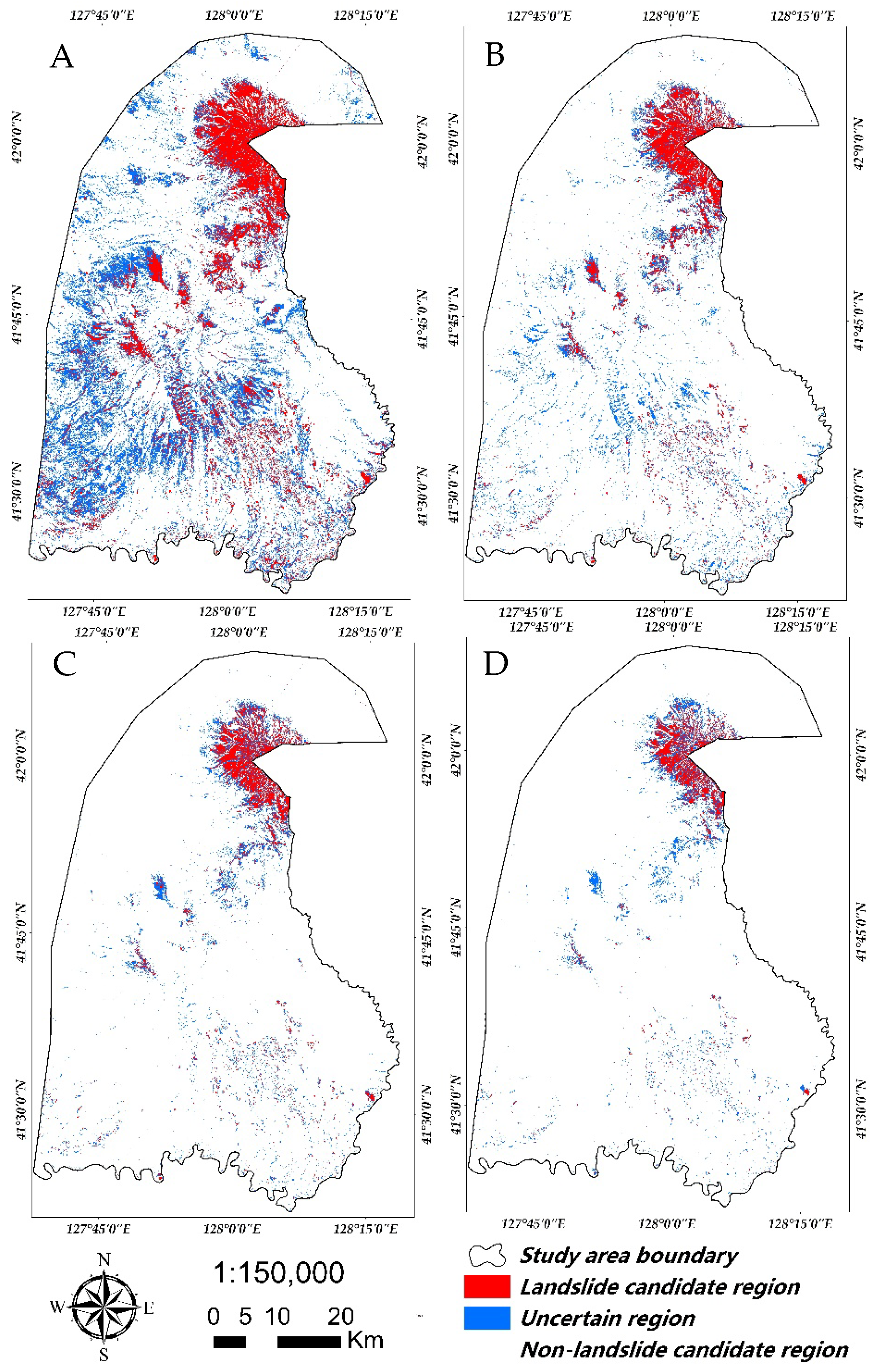
2.2.2. Change Detection-Based Multi-Thresholding

(1) Generation of the difference image

The DI is generated using the CVA proposed by Lambin and Strahler [38] and defined as follows:

$$\mathsf{\rho }\left(I\right)={\left[{\displaystyle \sum }_{b=1}^n{\left(I_{t_1}-I_{t_2}\right)}_b^2\right]}^{1/2}$$

(1)

where $I_{t_1}$ and $I_{t_2}$ are the pixel values of pixel $I$ at times $t_1$ and $t_2$ respectively, $b$ is the band number, $n$ is the total band number, and $\mathsf{\rho }\left(I\right)$ is the changing value of pixel $I$. Usually, a larger value of $\mathsf{\rho }\left(I\right)$ indicates that a big change occurred in pixel $I$ from $t_1$ to $t_2$. Thus, pixels with a greater value represent landslide candidate regions, but some incorrect landslide candidate regions are often determined in error due to phenology variations and illumination differences. Merely using DI cannot produce candidate regions; therefore, further efforts are required to generate candidate regions for the entire area. To address this problem, the multi-thresholding method was used to obtain candidate regions. Meanwhile, LSA was used to identify landslide candidate regions because it shows where landslides are prone to occur and the possibility of occurrence considering the topographic/geomorphologic, geologic, and land cover background information. However, it also shows the susceptibility of the entire study area; therefore, to reduce the user load, candidate regions of landslides and non-landslides were obtained using an effective multi-threshold method.

(2) Generation of candidate regions

To further refine the errors mentioned previously, a threshold method presented by Chuvieco [39] was employed in this study. To extract landslide candidate regions from error regions in the DI, the changing value of the change vector in each pixel was compared with a given multi-threshold. Thus, the candidate regions of landslides, non-landslides and uncertain areas were generated by the following multi-threshold method:

$$I_{DI}=\{\begin{array}{cc}landslidecandidateregion,& \hfill if\mathsf{\rho }\left(I\right)\ge \mathsf{\mu }+\left(T+\Delta T\right){\ast \mathsf{\sigma }}_{DI}\\ uncertainregion,& \hfill if\mathsf{\mu }+\left(T+\Delta T\right){\ast \mathsf{\sigma }}_{DI}>\mathsf{\rho }\left(I\right)>\mathsf{\mu }+T{\ast \mathsf{\sigma }}_{DI}\\ non-landslidecandidateregion,& \hfill if\mathsf{\rho }\left(I\right)\le \mathsf{\mu }+T{\ast \mathsf{\sigma }}_{DI}\end{array}$$

(2)

where $I_{DI}$ indicates the category of pixel $I$, $\mathsf{\rho }\left(I\right)$ indicates the changing value of pixel $I$, $\mathsf{\mu }$ and ${\mathsf{\sigma }}_{DI}$ are the mean and standard deviation value of whole area, respectively. T and ∆T are the parameters that often needs to be tuned in different situations. According to Equation (2), if the pixel change values $\mathsf{\rho }\left(I\right)$ are greater than or equal to $\mathsf{\mu }+\left(T+\Delta T\right){\ast \mathsf{\sigma }}_{DI}$, the pixels are classed into landslide candidate regions; if they are smaller than or equal to $\mathsf{\mu }+T{\ast \mathsf{\sigma }}_{DI}$, they are classed into non-landslide candidate regions; otherwise they are classified into uncertain regions. In this way, the final landslide candidate region can be obtained as shown in following Section 3.1.

As well as the multi-threshold method, another binary threshold method often used in CVA was presented by Xian, Homer and Fry [40], which involved only one adjustable parameter ($\mathsf{\alpha }$). However, according to the two research papers proposed by Li et al. [37,41], the multi-threshold method is more suitable for CVA in landslide mapping research than the binary threshold method, which divides weak spectral change regions into landslide candidate regions; the boundaries of weak spectral change regions are more blurred in the multi-threshold method, reducing the misclassified area. Therefore, the $T$ and $\Delta T$ parameters play critical roles in the threshold judgement in Equation (2). In order to determine the threshold, 10 tests were conducted with T and ∆T parameters of 0.5 and 0.5; 1 and 1; 1.5 and 1.5; and 2 and 2, respectively (Figure 4). And 2 and 1.5; 1.5 and 2; 2 and 1; 2 and 0.5; 1.5 and 1; and 1.5 and 0.5, respectively (Figure 5). For $T$ and $\Delta T$ of 2 and 1, we observed the lowest number of over-identified regions; therefore, these values were used for $T$ and $\Delta T$ in this study.

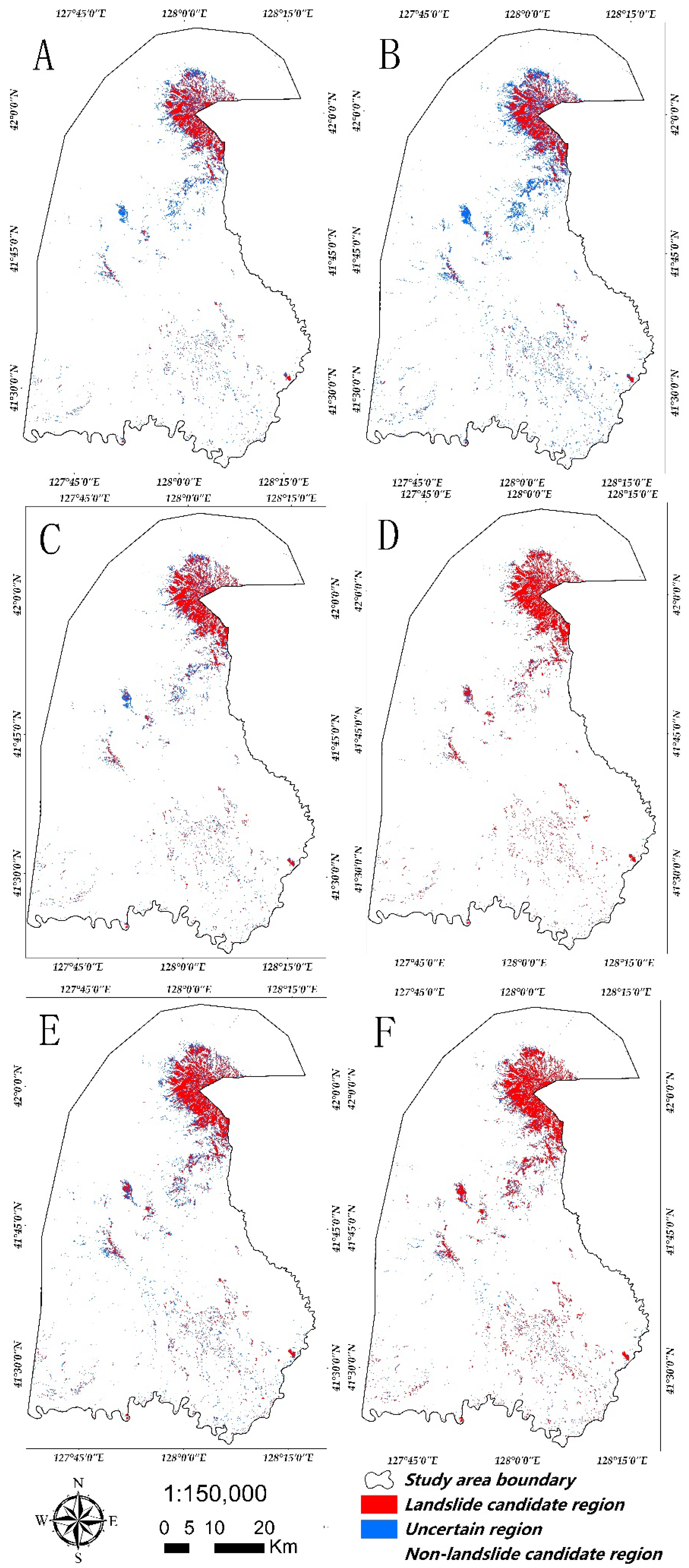
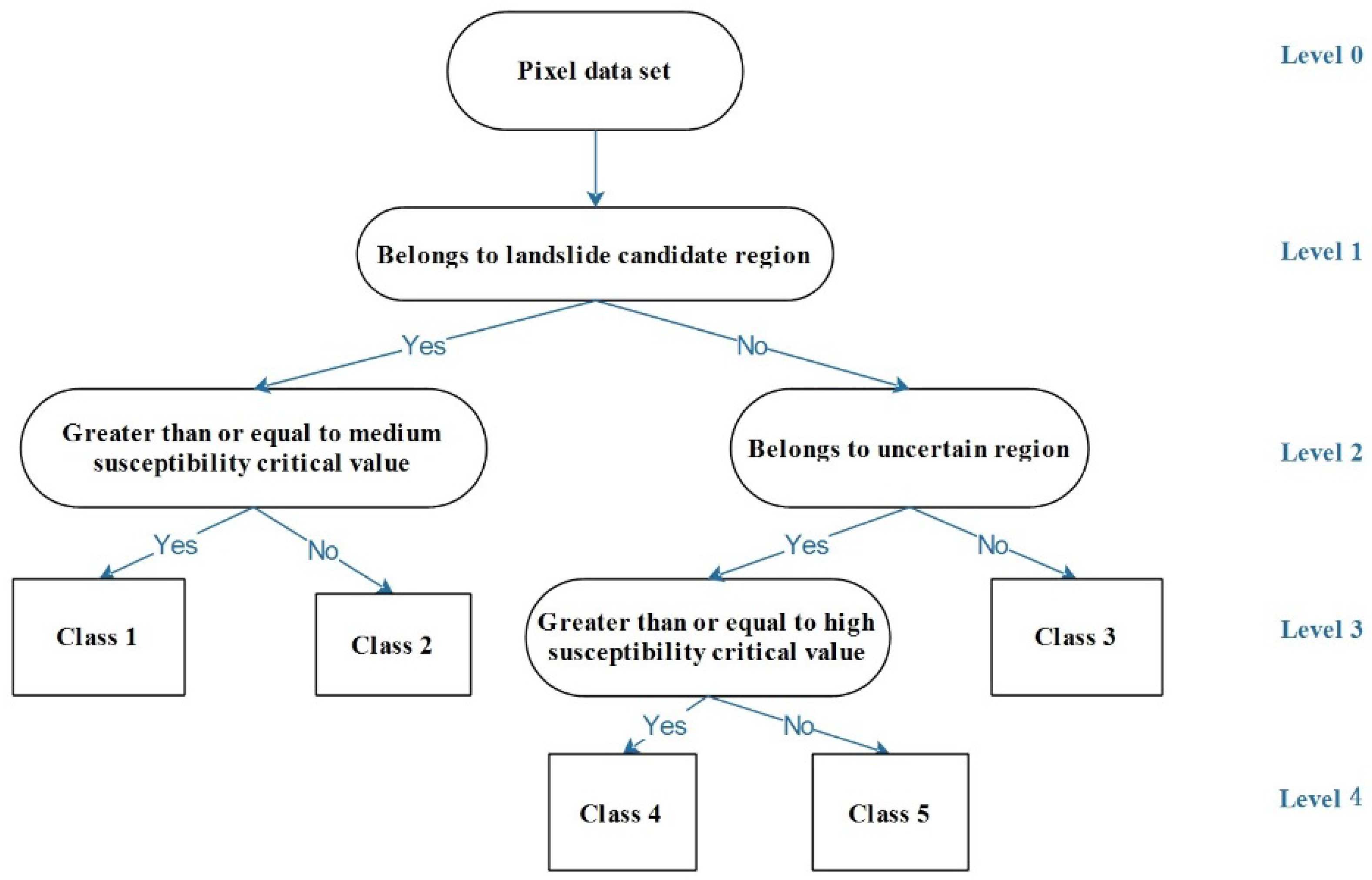
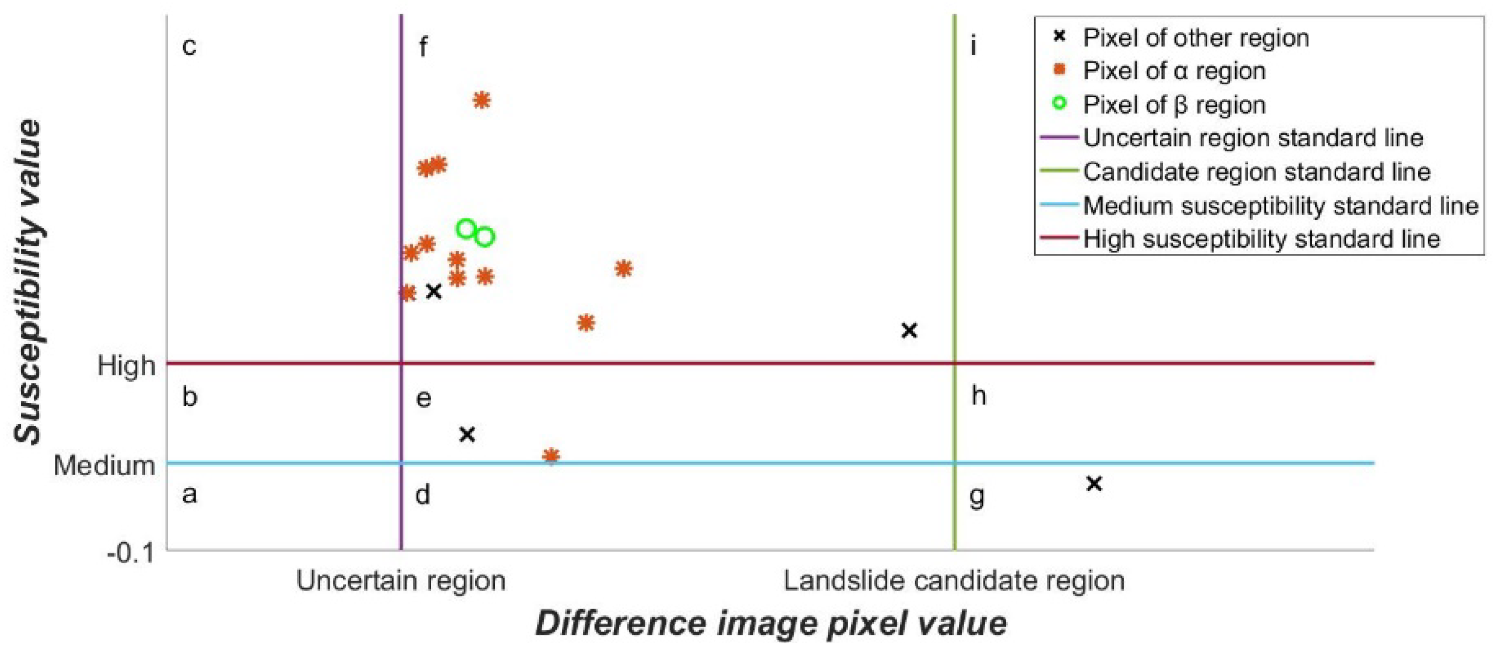
2.2.3. Susceptibility Analysis-Based Identification

Based on the candidate regions obtained in the former step, LSA was conducted to further refine the results. From the definition of susceptibility mentioned above and considering the detailed topography/geomorphology, geology, and land-cover background information, the LSA can directly show the possibility of landslide occurrence inside the candidate region, thus providing a criterion for landslide identification.

(1) Calculation based on random forest mode

Among all the susceptibility analysis methods, the RF model is well known due to its excellent prediction performance [42,43,44]. Thus, we employed the RF model to calculate the susceptibility of the entire study area. The random forests multivariate statistical technique is an implementation of the Bayesian tree or binary classification tree, as it considers an ensemble (i.e., a forest) of $\mathrm{n}$ trees to multiply the efficiency and predictive capability accordingly [45]. The random forest model uses the bagging technique (i.e., bootstrap aggregation) to extract multiple samples of the conditioning parameter from the training conditioning parameters dataset and utilize each sample to build a decision tree model to assemble the prediction result of multiple trees, employing voting to obtain the final prediction result. The probability of an unselected sample in the training dataset is ${\left(1-\frac{1}{N}\right)}^N$, where $N$ is the number of samples in the training dataset. These data are called out-of-bag (OOB) data, which are used to calculate the error of the model (i.e., OOB Error) and are equal to the standard deviation error between predicted and observed values.

Before using the random forest to calculate susceptibility, we performed several steps to reduce disturbances caused by the data. For this, the susceptibility must be calculated in order to conduct identification, with the help of the CDT result in the following step. The susceptibility is needed to display the probability of landslide occurrence between the years of 2014 and 2016, in other words, the susceptibility is required to represent the prediction rate of landslide occurrence after 2014. Therefore, we did not include landslide region data between 2014 and 2016 in the training sample used to calculate susceptibility (if these data had been included, the susceptibility of the corresponding regions would be too high and would not represent the possibility of landslide occurrence). A pre-landslide topographic map and other data were used to obtain 12 parameters, and were combined with the remaining data of the 141 landslides to calculate susceptibility in order to represent the possibility of landslide occurrence more realistically. Only in this way can we use this result, combined with the CDT results, to identify landslides. Additionally, considering LULC in the susceptibility calculation helps to remove incorrect landslide candidate regions caused by variations in land cover from buildings, farmland, and construction sites. In this study, we implemented 500 decision trees to calculate the susceptibility of the study area, using a voting process to achieve the final result.

(2) Evaluation based on the receiver operating characteristic (ROC) method

Performance of the prediction accuracy for landslide susceptibility can be assessed using the receiver operating characteristic (ROC) curve method, which plots the sensitivity (i.e., the true positives) versus the specificity (1 specificity, or the false positives) used to measure the goodness-of-fit of the model prediction. The area under the curve (AUC) value represents the area under the ROC curve, which is used to quantitatively show the results of the ROC [46]. The AUC varies from 0.5 (diagonal line) to 1, with higher values indicating better predictive capability of the model. AUC values less than 0.7 indicate poor predictive ability; values between 0.7 and 0.8 represent moderate predictive ability, values between 0.8 and 0.9 represent good predictive ability and values >0.90 are typical of excellent predictive ability of the model. However, recent studies have shown that models with similar AUC values can produce very different susceptibility maps.

2.2.4. Candidate Region Identifications

Using the susceptibility value and difference image pixel value as the X and Y axis of a scatter plot directly illustrates the relationship between these values for all pixels. We then imposed several conditions to divide the pixels into five classes (Figure 6).

The thresholds for landslide candidate regions and uncertain regions are given by Equation (2); the natural breaks method was used to obtain the high and medium susceptibility thresholds (the susceptibility threshold is used for reference purposes). The proposed method aims to identify landslides over the entire study area; thus, the susceptibility and CD thresholds were set for the entire study area. Three sub-areas were processed to represent the results of the SCDT method more clearly; these sub-area thresholds must be the same as for the entire study area in order to represent the actual results of the entire study area.

When pixels belonging to class 1 and 4 account for 50% of all pixels from the same region, this region is classified as a landslide region is. When pixels belonging to the other classes account for 50% of all pixels from the same region, this region is classified as a non-landslide region. The accuracy of this approach was verified using the method proposed in Section 2.2.5.

2.2.5. Experimental Setup

For a quantitative evaluation and to verify the advantages of the proposed method, the mapped landslides were compared with the reference boundary provided by JIGEM, using the following three evaluation indices:

$$Correctness=\raisebox{1ex}{$P_{lm}$}\!\left/ \!\raisebox{-1ex}{$P_l$}\right.$$

(3)

$$Completeness=\raisebox{1ex}{$P_{lm}$}\!\left/ \!\raisebox{-1ex}{$P_r$}\right.$$

(4)

$$Quality=\raisebox{1ex}{$P_{lm}$}\!\left/ \!\raisebox{-1ex}{$(P_l+P_{rum})$}\right.$$

(5)

where $P_{lm}$ is the total pixel number of identified landslide regions that match the reference maps, $P_r$ is the total pixel number of reference landslide regions, $P_l$ is the total pixel number of the identified landslide regions, and $P_{rum}$ is the total pixel number of reference landslide regions that do not match the identified landslide regions. These three indices validated the results through three aspects, i.e., the matching degree of the identification result with the reference boundary; the matching degree of identification results inside the reference boundary with the actual landslide area; and the comprehensive matching degree. These three indices are designed for a pixel-based method, which fits with our proposed method; thus, they quantify the performance of the method in a simple and straightforward manner.

3. Results

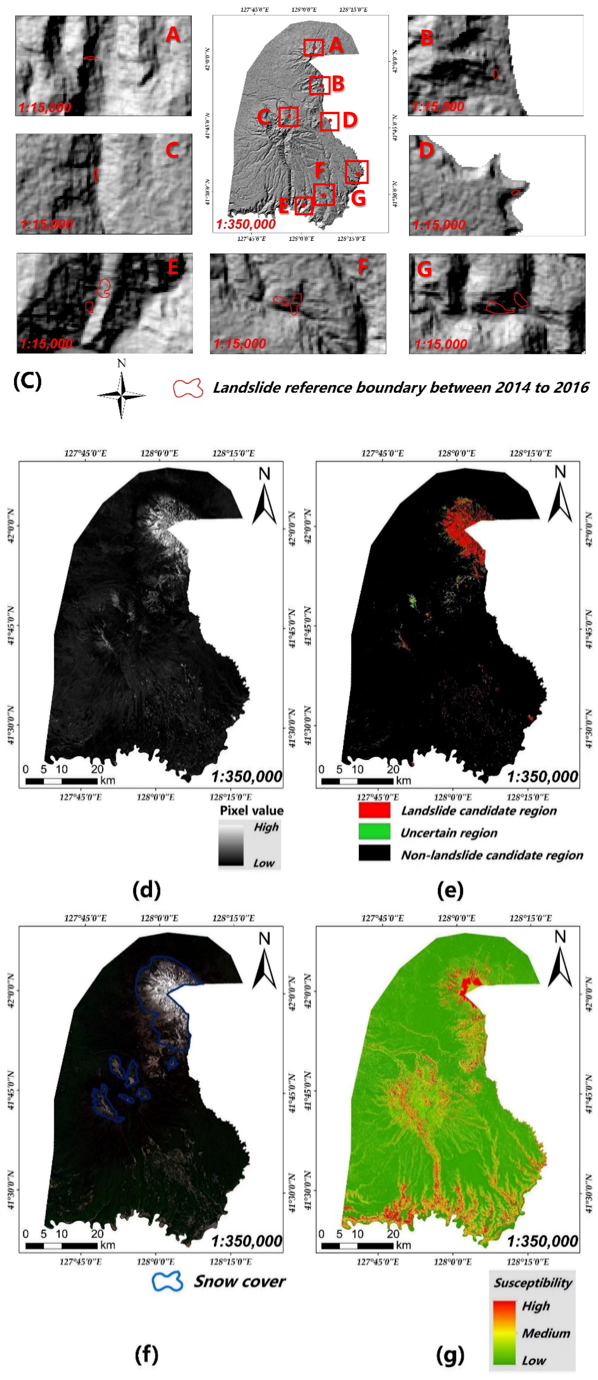
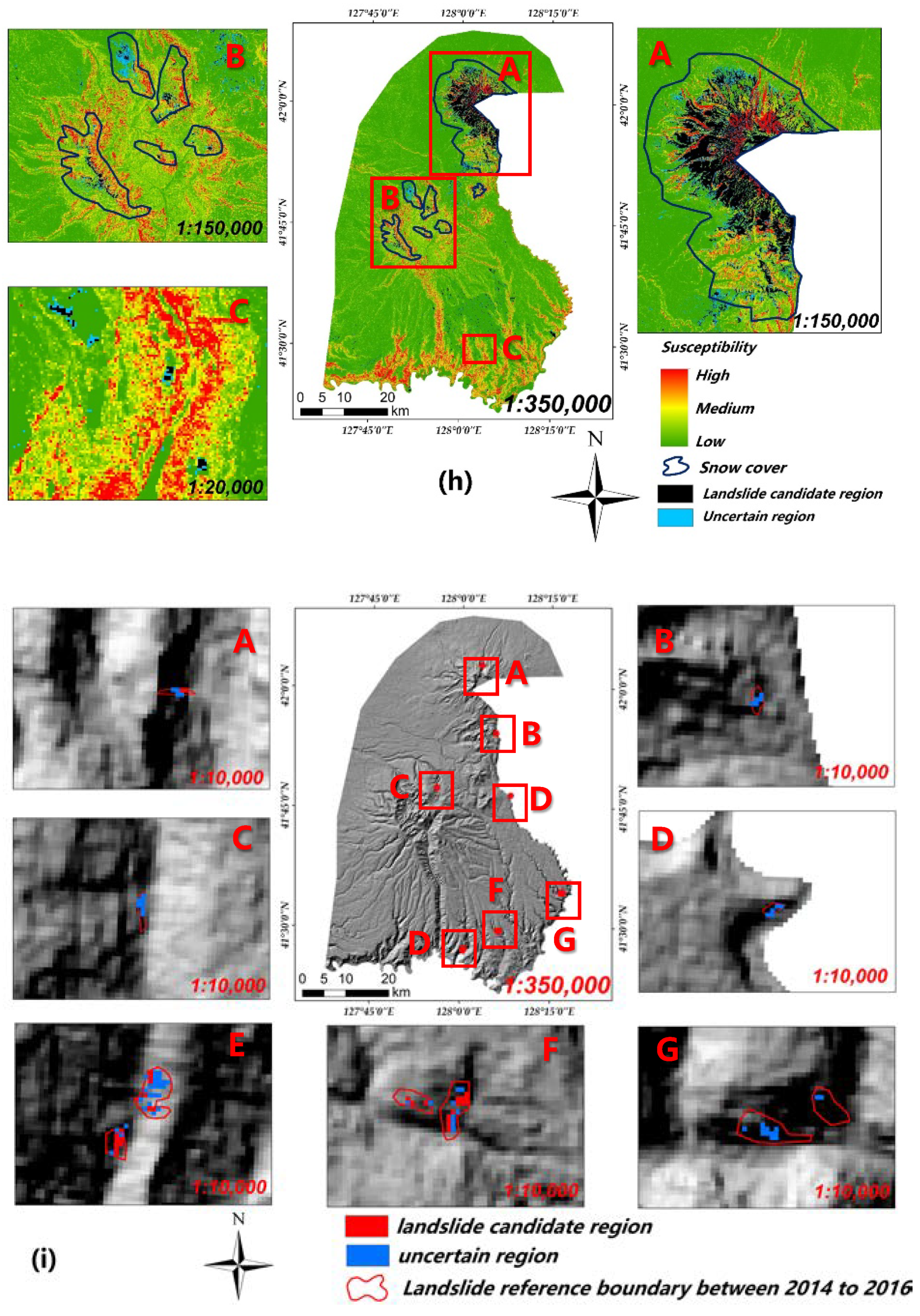
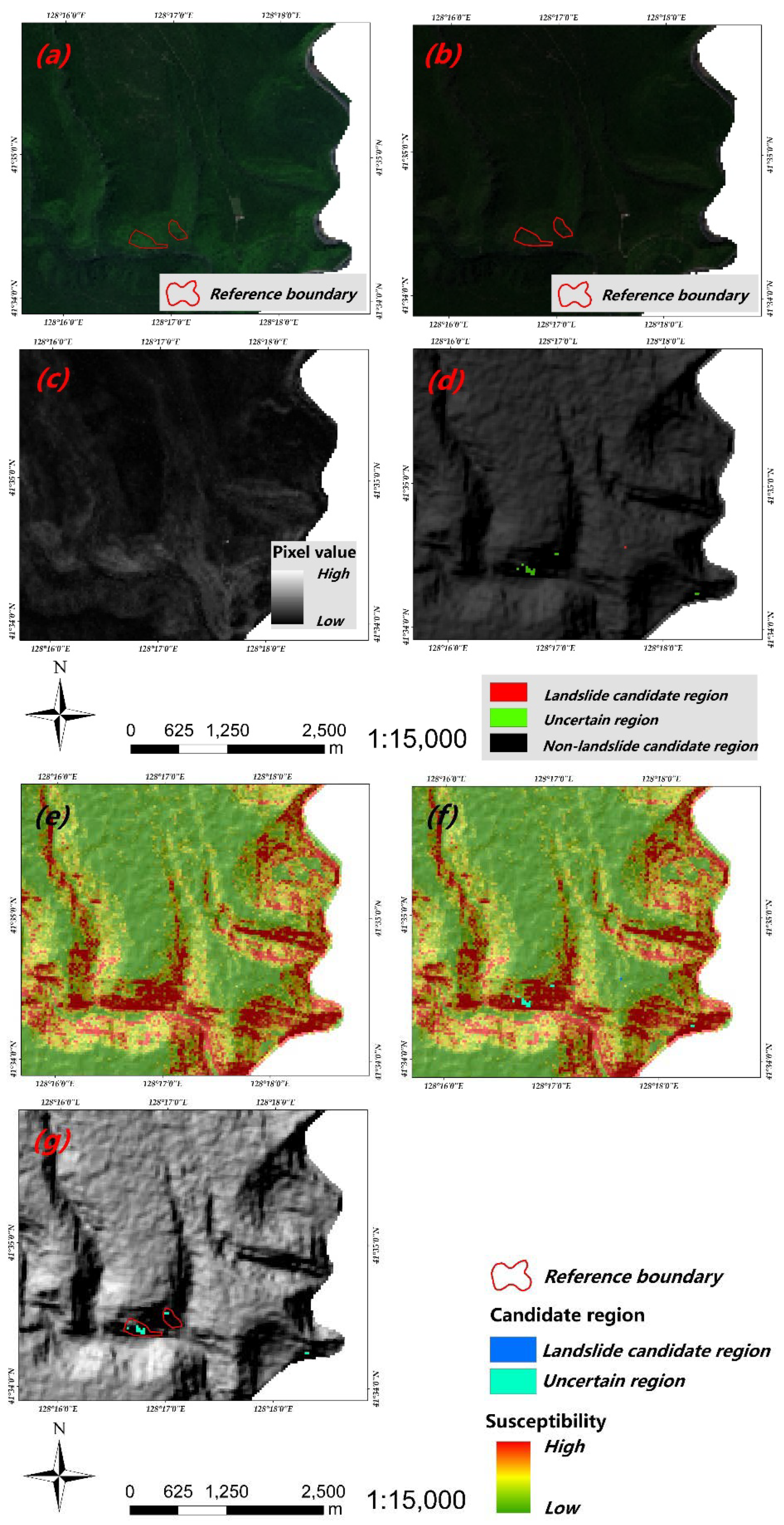
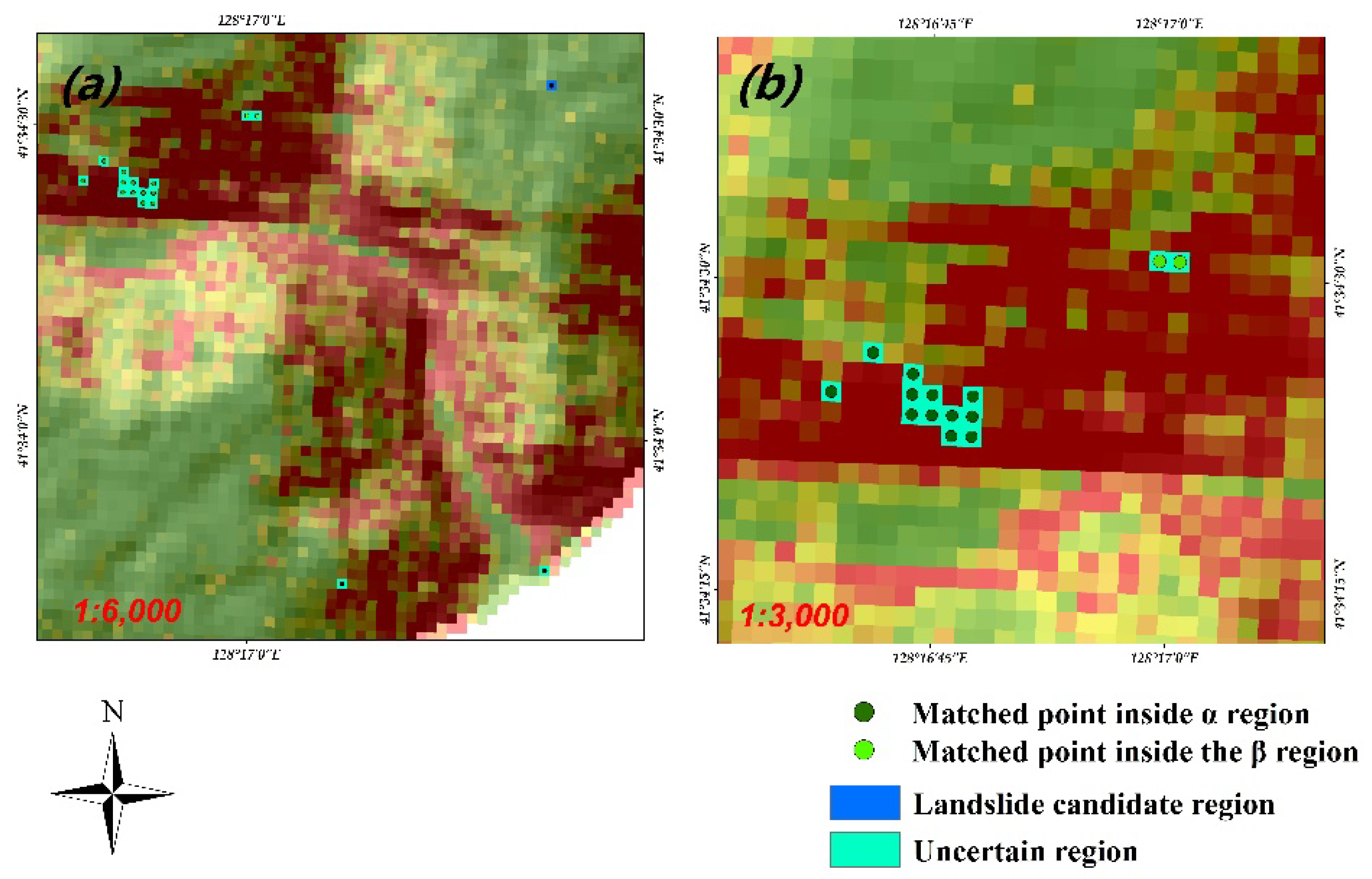
3.1. Qualitative Evaluation

Firstly, the proposed methods were applied to the entire study area, the results of which are presented in Figure 7a–i. Pre- and post-event images are shown in Figure 7a,b. According to the landslide inventory (reference boundary) supplied by JIGEM, from May 2014 to May 2016, 10 landslides occurred in the study area (Figure 7c). It is difficult to quantify the performance of the methods based on such limited data; therefore, we performed the SCDT method using pixels as the basic unit. As there are 306 pixels inside these 10 landslides, we obtained sufficient data to support and validate our method.

These 10 landslides occurred in regions with different terrain, positions and land cover which led to each landslide having a different shape. As mentioned before, the CDT is very sensitive to relatively high pixel change values. However, generating the difference image (Figure 7d) and calculating threshold enable the CDT to effectively display the regions where changes occurred between 2014 and 2016. Because of urban areas, farmland areas, construction sites, ice or snow cover, and road changes, too many candidate regions appeared in the study area between 2014 and 2016 (Figure 7e). These regions were temporarily classed as landslide candidate regions and uncertain regions according to Equation (2) prior to further processing.

Due to the existence of snow cover changes in the study area, we needed to determine the snow cover (Figure 7f) change area through visual interpretation and compare it with the CDT result to eliminate disturbance regions. Moreover, a crucial step in the landslide identification involved calculating the susceptibility results of the entire study area using the RF model (Figure 7g). The OOB result of the LSA shows that, after establishing 250 trees, the error rate of the RF becomes stable and small (Figure 8). We then, we cross-validated the susceptibility results using the ROC method.

We then used the testing dataset to calculate the ROC of the susceptibility results (Figure 9). After establishing 500 decision trees, the error rate of the RF model is the lowest and the accuracy of the RF model is 0.9391 (AUC = 0.9391), indicating that the susceptibility result for the entire study area calculated by the RF model is excellent and extremely predictive.

As previously mentioned, the results of the CDT are used as reference regions to further identify actual landslide regions based on the susceptibility analysis results (Figure 7h), which will ensure that SCDT results are more precise than CDT results.

According to Figure 7i, after conducting identification using SCDT, the candidate regions of the entire study area become much smaller than the CDT result, which reduces most of the interference regions and retains all actual landslide regions. Under 1:550,000 scale conditions, it is difficult to clearly display the SCDT result so we display the SCDT results of the 10 landslide region at 1:10,000 scale. In the following subsections, landslide identification are further examined in the three sub-areas, which experienced the six largest landslides between 2014 and 2016.

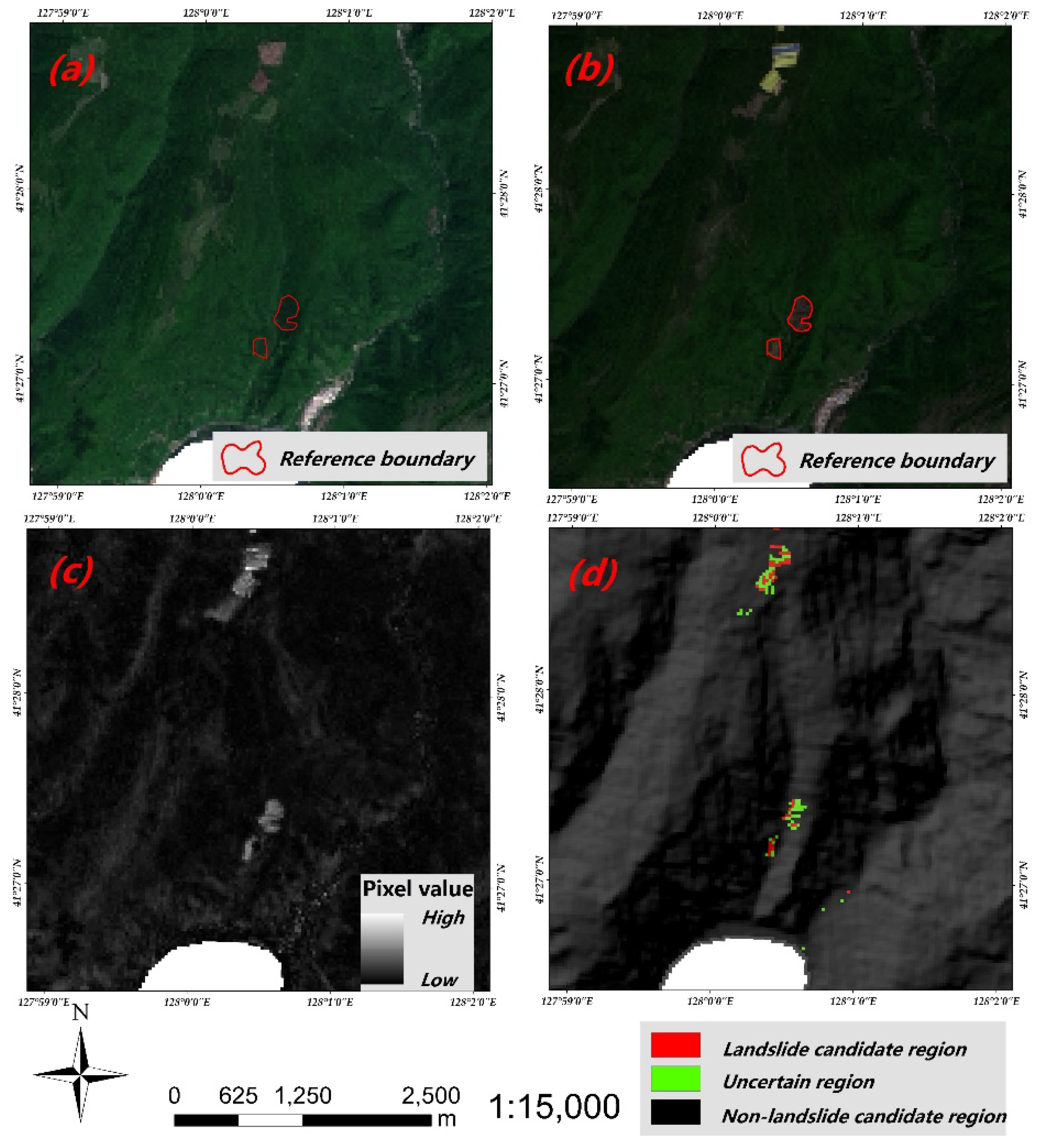
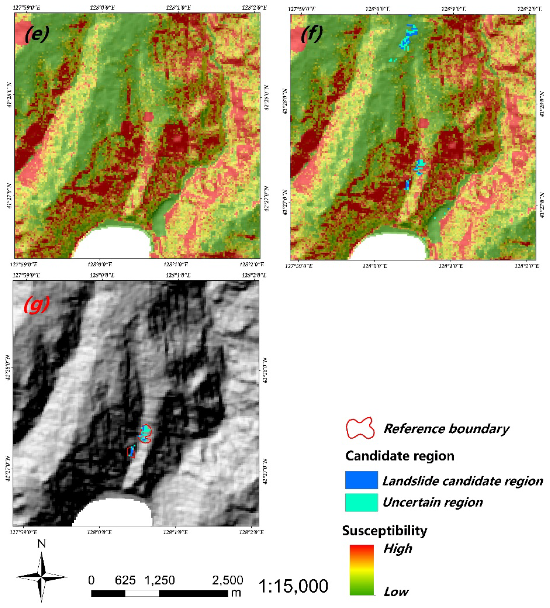
3.1.1. Sub-Area A

The landslide identification results in sub-area A are presented in Figure 10a–g. Sub-area A is located in the southern part of the study area close to the boundary (Figure 1); a small part of the sub-area belongs to farmland and villages, and the majority is forest land. During the period 2014 to 2016, two rotational landslides occurred inside this sub-area according to the inventory, as shown in Figure 10a,b. There are total of 82 pixels inside these two landslide boundaries, slope ranges of 6° to 42°, in which 90% of the pixels are higher than 15°, and the mean slope angle is approximately 31°, one is westward and the other is eastward. Therefore, from the slope conditions, landslides are likely to occur in these two regions. Meanwhile, there is no human disturbance around these two regions; no railway, highway or human residence. There are obvious changes and spectral differences inside the reference boundary. In Figure 10c,d, the DI and thresholding results show change regions inside sub-area A, and the CDT results alone cannot obtain accurate landslide regions; many incorrect candidate regions are observed around the landslide regions. After obtaining the susceptibility using the RF model (Figure 10e), we overlapped the two results (Figure 10f) and conducted landslide identification to eliminate the incorrect candidate regions and obtain the final results (Figure 10g).

Different colors were assigned to the pixels inside the two landslide reference boundaries to clarify the results, assigned dark green color to α region and assigned light green color to β region, while pixels outside the boundary were colored black (Figure 11a). α and β regions are the code name of two landslide regions occurred in this sub-area.

Figure 12 shows all pixels inside sub-area A as a scatter plot, indicating that four lines split the plot in to nine districts; two horizontal lines are based on the high and medium thresholds of susceptibility and two vertical lines are based on the uncertain region and landslide candidate region thresholds. The X and Y axes represent the pixel susceptibility value and difference image value respectively; if the pixel is closer to the upper right area of the plot, it is more likely to belong to a landslide. According to Section 2.2.4, a pixel located in district i and h belongs to class 1, a pixel located in district g belongs to class 2, a pixel located in district a, b, and c belongs to class 3, a pixel located in district f belongs to class 4, and a pixel located in district e and d belongs to class 5.

For region α, only one pixel belongs to class 2, five pixels belong to class 5, and the remaining 27 pixels belong to class 1 and class 4, accounting 81.82% of all pixels in region α, which meets the standard mentioned in Section 2.2.4. Thus, this region is classed as an actual landslide. For region β, no pixels belong to class 2, two pixels belong to class 5, and the other 12 pixels belong to class 1 and class 4, accounting 85.71% of the region β. This region is therefore also identified as an actual landslide. For the other region, only one pixel belongs to class 1, so it is clearly a non-landslide area (Figure 11b). Sub-area A includes three regions identified as candidate regions (including actual landslide regions) by the CDT method (Figure 10d). Apart from the two actual landslide regions located in the middle of sub-area A, Figure 10a,b indicates that other candidate regions are caused by vegetation cover changes to farmland and road cover changes.

3.1.2. Sub-area B

The landslide identification results in sub-area B are presented in Figure 13a–g. Sub-area B is also located in the southern part of the study area, but closer to the internal area than sub-area A (Figure 1); it comprises many villages and farmland. During the period 2014 to 2016, two planar shallow landslides occurred in this sub-area. Inside these two landslide boundaries there are total of 77 pixels, slope ranges of 4° to 37°, in which 90% of the pixels are higher than 15°, and the mean slope angle is 24°, from this we can determine that the slopes of these two regions are relatively gentle. However, there are highways near these two regions, and it may be that human disturbance caused a slope failure. Figure 13a,b reveals obvious changes and spectral differences inside the reference boundary. Similar to sub-area A, many incorrect candidate regions exist around the landslide regions. We conducted landslide identifications to eliminate the incorrect candidate regions and obtain the final results (Figure 13g).

Different colors represent pixels inside the two landslide reference boundaries and black indicates pixels outside the boundary (Figure 14a). α and β regions are the code name of two landslide regions occurred in this sub-area.

All pixels inside sub-area B are shown as a scatter plot in Figure 15. For region α, 12 pixels belong to class 1 and class 4, accounting for 60% of all pixels. For region β, no pixels belong to class 2, six pixels belong to class 5, and the remaining 25 pixels belong to class 1 and class 4, accounting for 80.65%. Both of these regions are therefore identified as actual landslides. For the other region, only 1% of all pixels are belong to class 1, so it is easily determined as a non-landslide, revealing the final result of our proposed method (Figure 14b). Many regions in sub-area B are identified as candidate regions (including actual landslide regions) by the CDT method (Figure 13d). Apart from the two actual landslide regions, almost all other candidate regions are caused by vegetation cover changes related to farmland or road cover changes (Figure 13a,b). A small number of other candidate regions exist for other reasons; through identification using the susceptibility results and CDT results, we eliminated these regions and retained only the actual landslide regions.

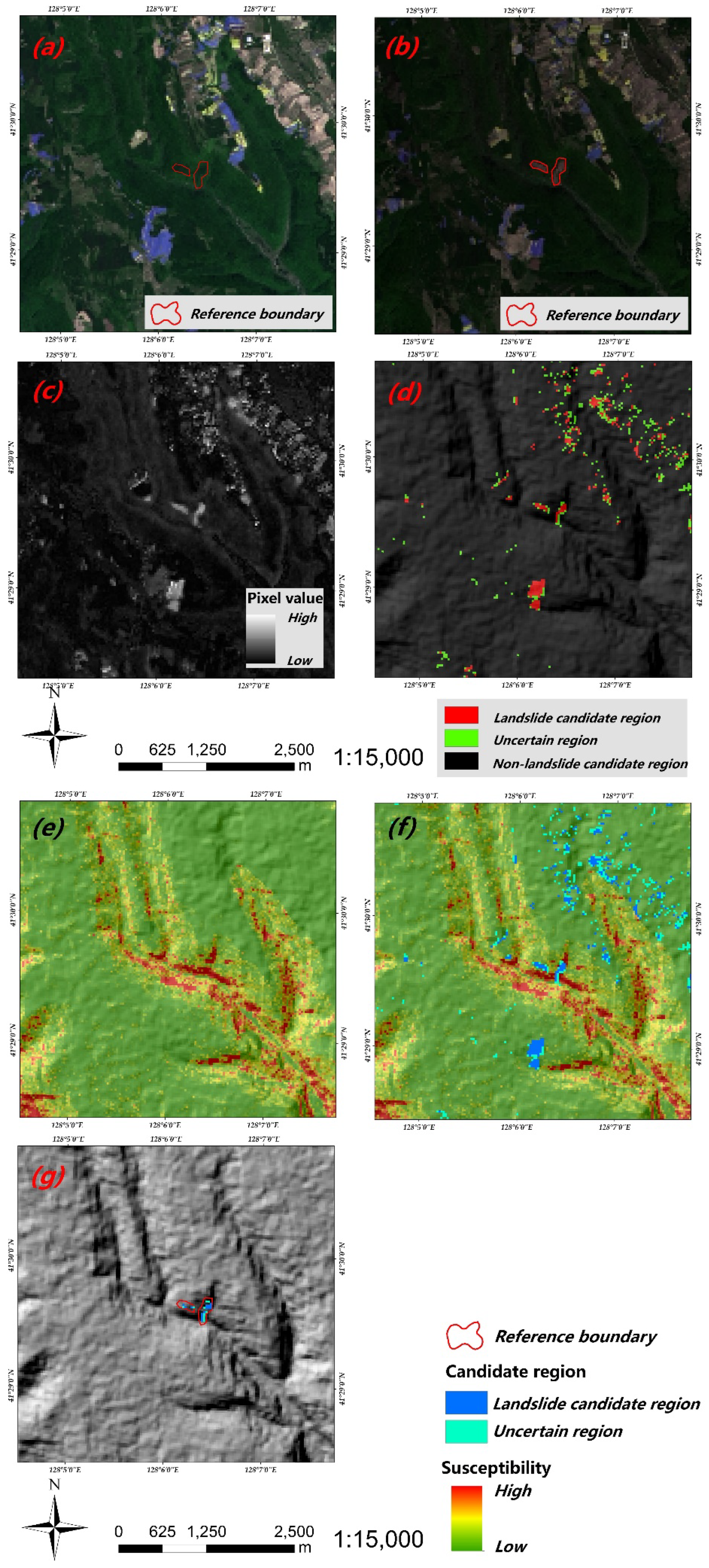
3.1.3. Sub-area C

The landslide identification results of sub-area C are presented in Figure 16a–g. This sub-area is located in the southeastern part of the study area, close to the boundary (Figure 1), and is completely made up of forest land, with no construction sites or farmland. The pre- and post-event images are shown in Figure 16a,b, respectively. Slight changes occur inside the reference boundary and the spectral differences are not obvious; therefore, it is hard to visually determine the differences. Two rotational landslides occurred inside this sub-area, both of which were northward. There are 104 pixels inside these two boundaries, slope ranges of 13° to 60°, of which almost 98% of the pixels slope angle are higher than 15°, and the mean slope angle is 37°. From these conditions, it is likely landslides will occur within these two regions. SCDT was then conducted to identify the landslides and obtain the final results (Figure 16g).

Different colors represent pixels inside the two landslide reference boundaries and black indicates pixels outside the boundary (Figure 17a). α and β regions are the code name of two landslide regions occurred in this sub-area.

The scatter plot of all pixels inside sub-area C is shown in Figure 18. For region α, 11 pixels belong to class 1 and class 4, accounting for 91.67% of all pixels in the region. For region β region, all pixels belong to class 1 and class 4. Thus, both are identified as actual landslides, leading to the final result in Figure 17b. A few regions of sub-area C are identified as candidate regions (including actual landslide regions) by the CDT method (Figure 16d). Apart from the two actual landslide regions, all other candidate regions are caused by slight vegetation cover changes (Figure 16a,b). Through identification using the susceptibility results and CDT results, we eliminated these regions and retained only the actual landslide regions.

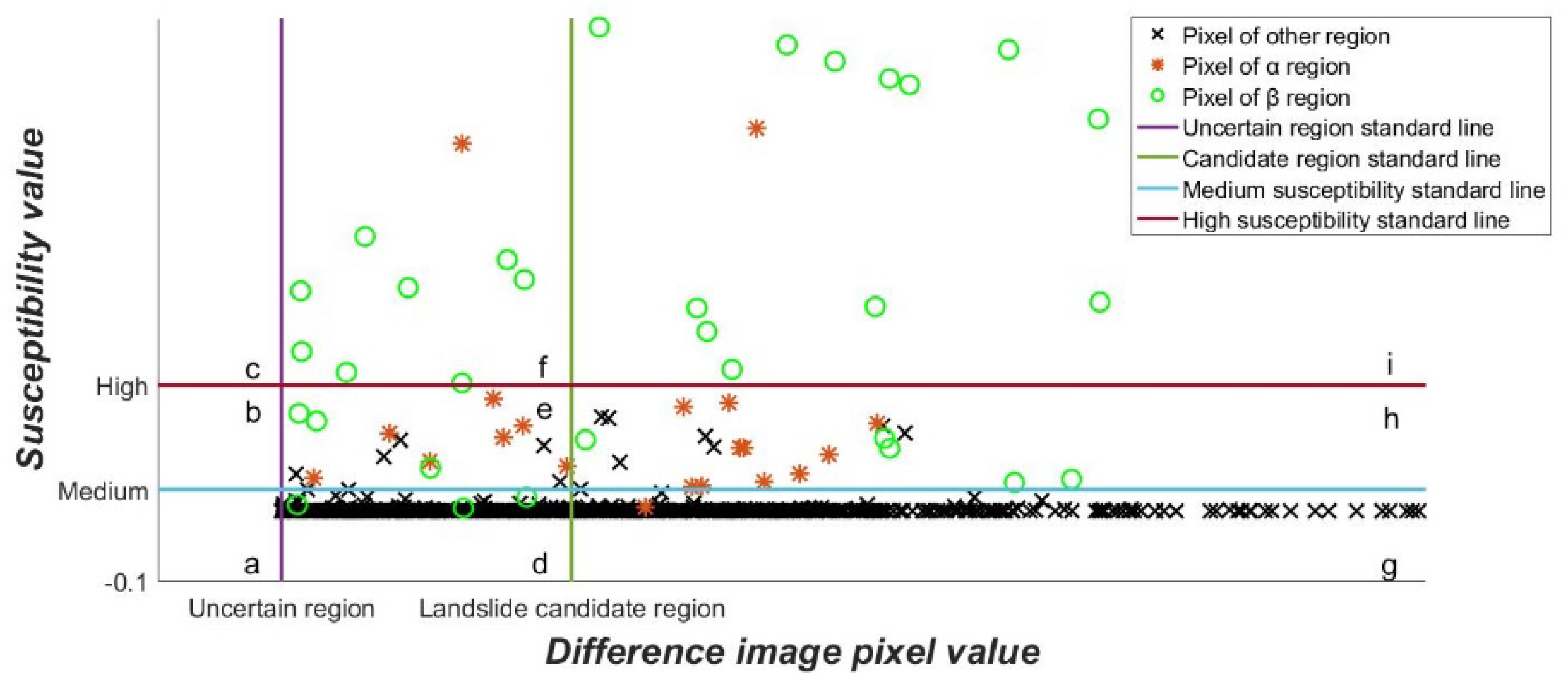
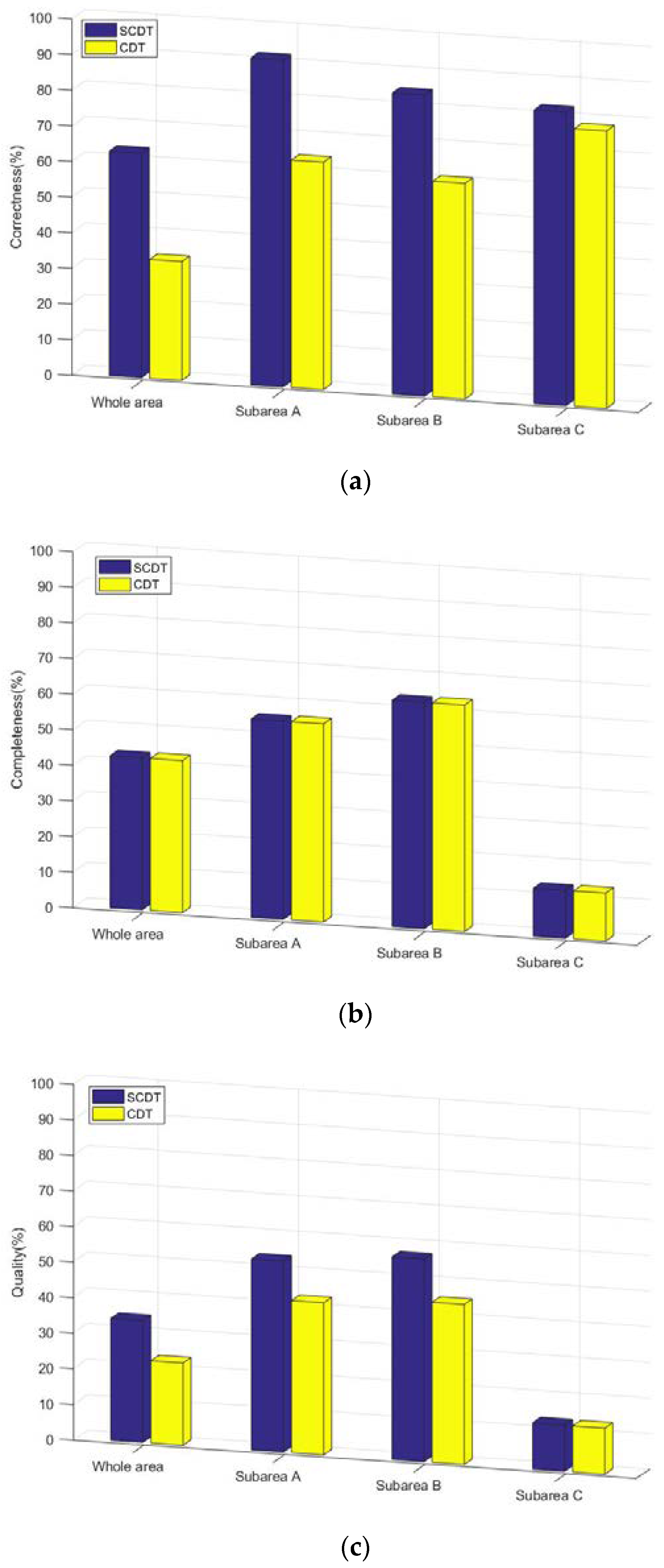
3.2. Quantitative Evaluation

For the quantitative evaluation, we used three methods to assess the reliability and accuracy of the proposed method, then compared the SCDT results with the masked CDT results to verify the effectiveness of the method. The final quantitative evaluation results for completeness, correctness, and quality are presented in Figure 19a–c. Correctness is designed to verify the matching degree of the identification result with the reference boundary. The correctness of SCDT exceeds the masked CDT in all four areas because SCDT conducts more comprehensive identification to further refine the results of CDT, which uses LULC to eliminate non-actual landslide regions. The SCDT results for the entire study area and all three sub-areas are improved by 29.60%, 27.90%, 23.99%, and 4.57% respectively (

Table 1. Increasing rate of the proposed method.

Study Areas	Methods	Evaluation Indices (%)
		Correctness	Completeness	Quality
Whole area	SCDT	62.93%	42.72%	34.22%
	CDT	33.33%	42.72%	23.08%
	Increasing rate	29.60%	0%	11.14%
Sub-area A	SCDT	91.67%	55.70%	53.66%
	CDT	63.77%	55.70%	42.72%
	Increasing rate	27.90%	0%	10.94%
Sub-area B	SCDT	84.48%	63.64%	56.98%
	CDT	60.49%	63.64%	44.95%
	Increasing rate	23.99%	0%	12.03%
Sub-area C	SCDT	82.35%	13.46%	13.08%
	CDT	77.78%	13.46%	12.96%
	Increasing rate	4.57%	0%	0.12%

).

The completeness results are quite different from the correctness results; the completeness of SCDT is exactly the same as that of CDT (Table 1), as seen in Figure 19b. This is because CDT is designed to verify the matching degree of identification results inside the reference boundary with the actual landslide area. The quality of SCDT slightly exceeds that of CDT, as shown in Figure 19c. The quality is designed to verify the overall effect of the identification method, considering both the correctness and completeness of identification. Thus, due to the difference in correctness values, the quality of the SCDT method is slightly improved from that of the CDT method by 11.14%, 10.94%, 12.03%, and 0.12%, respectively (Table 1).

4. Discussion

Our proposed SCDT method is quantitatively compared with the masked CDT and verified. The correctness of the SCDT method shows a significant improvement; in all four areas it is above 60% and in three sub-areas it is above 80%, clearly exceeding the masked CDT method. Using land-cover/land-use layers to mask the CDT results did not eliminate all incorrect candidate regions, including those exhibiting vegetation cover changes. Therefore, these regions were identified as landslide regions, which led to a decrease in identification accuracy. The susceptibility results comprehensively displayed the conditions of some regions, not only from the aspect of land cover/land use, but also according to slope degree and terrain conditions, among others. Thus, the SCDT method also considered more comprehensive background information during identification; i.e., the spectral and spatial information of the regions. The SCDT method eliminated candidate regions based on this information, enabling a more accurate identification of landslides. As the goal of this study was to identify rather than map landslide regions, the completeness values are less important. The quality index was designed to verify the overall effect of the identification method, and shows a slight improvement along with the improvement in correctness. SCDT performed very well for the identification of landslides in three sub-areas, but decreased a lot when it was conducted on the scale of a whole study area.

We first used only rotational and planar shallow landslide data to calculate the susceptibility. Therefore, the results are only focused on the identification of rotational or planar shallow landslides. However, inside the study area, several debris flows also occurred, and our proposed method identified these debris flows as actual landslides. This one reason caused the decrease in performance when applied to the whole study area. There may also be some error in the LULC data which could cause misidentification. Meanwhile, the reference boundary described the final shape of the landslide body, but also contained some areas which did not belong to the trigger areas. As these non-trigger areas were taken as part of the input data, the accuracy of the LSA result was reduced. Although 93% of the AUC value represented a relatively high prediction accuracy, almost 7% of the pixels’ value was miscalculated. Also, due to the existence of these wrong values, the accuracy of the SCDT identification result was reduced to an extent.

Visual evaluations of the three sub-areas revealed clear changes of landslide regions in sub-areas A and B shows. However, only slight changes in landslide regions were observed in sub-area C, which were hard to identify visually. This may be because landslides in sub-area C occurred near to the fetch time of the 2014 image, and the vegetation cover was restored during 2014–2016. However, the CDT method still detected slight changes between images from the two years and the SCDT method further confirmed these regions as landslide regions. For sub-area A, the SCDT method eliminated almost all farmland changes and road changes and retained the landslide regions. The candidate regions inside sub-area B were not only caused by farmland changes, road changes, and construction changes but also by vegetation cover changes. The SCDT method was able to retain the actual landslide regions in sub-area B. Because sub-area C was located in an isolated region, there were no areas of farmland, towns, or buildings, so there were few candidate regions in this sub-area.

5. Conclusions

This study provides an approach to landslide semi-automatic identification using the susceptibility-based change detection thresholding (SCDT) method, which integrates susceptibility analysis with the CDT method. From the perspective of quantitative evaluation, the results of the SCDT method are better than those of the masked CDT method. The SCDT method improves the accuracy of landslide identification and can reduce labor, time, and monetary investment. It shows excellent performance in regions where changes occurred frequently and also performs slightly better than the CDT method in isolated regions. It boasts a significant improvement in correctness, indicating very good performance regarding eliminating incorrect candidate regions, and a slight improvement in quality.

The SCDT method considers more comprehensive background information when conducting identification, therefore, the outcomes prove that the proposed method is valid and applicable. However, there are no improvements in the completeness of results compared to the CDT method; this is also caused by the low resolution of the Landsat 8 image. Therefore, future work should combine these results with the object-based approach to further improve boundary detection, increase the accuracy inside the boundary, and improve the correctness, quality, and completeness indicators. Meanwhile, a 10 m pixel resolution cannot represent the real topography conditions, but, due to the limitation of the data source and hardware conditions, we had no choice but to use pixels with a 10 m resolution to conduct our research. So, with the support of a better data source, we should further process this study using pixels with a higher resolution in future work. In addition, a 2D landslide identification is not sufficient to satisfy these research objectives; a 3D landslide identification should be used in future studies.

References

- Petley, D. Global patterns of loss of life from landslides. Geology. 2012, 40, 927–930. [Google Scholar] [CrossRef]
- Hervás, J.; Bobrowsky, P. Mapping: Inventories, susceptibility, hazard andrisk. In Landslides—Disaster Risk Reduction; Kyoji, S., Paolo, C., Eds.; Springer-Verlag: Berlin/Heidelberg, Germany, 2009; pp. 321–349. [Google Scholar]
- Van Den Eeckhaut, M.; Poesen, J.; Verstraeten, G.; Vanacker, V.; Moeyersons, J. The effectiveness of hillshade maps and expert knowledge in mapping old deep-seated landslides. Geomorphology 2005, 67, 351–363. [Google Scholar] [CrossRef]
- Guzzetti, F.; Mondini, A.C.; Cardinali, M.; Fiorucci, F.; Santangelo, M.; Chang, K. Landslide inventory maps: New tools for an old problem. Earth-Sci. Rev. 2012, 112, 42–66. [Google Scholar] [CrossRef]
- Metternicht, G.; Hurni, L.; Gogu, R. Remote sensing of landslides: An analysis of the potential contribution to geo-spatial systems for hazard assessment in mountainous environments. Remote Sens. Environ. 2005, 98, 284–303. [Google Scholar] [CrossRef]
- Del Soldato, M.; Di Martire, D.; Bianchini, S.; Tomás, R.; De Vita, P.; Ramondini, M.; Casagli, N.; Calcaterra, D. Assessment of landslide-induced damage to structures: The Agnone landslide case study (southern Italy). Bull. Eng. Geol. Environ. 2018, 1–22. [Google Scholar] [CrossRef]
- Dou, J.; Chang, K.; Chen, S.; Yunus, A.; Liu, J.; Xia, H.; Zhu, Z. Automatic case-based reasoning approach for landslide detection: Integration of object-oriented image analysis and a genetic algorithm. Remote Sens. 2015, 7, 4318–4342. [Google Scholar] [CrossRef]
- Huang, F.; Chen, L.; Yin, K.; Huang, J.; Gui, L. Object-oriented change detection and damage assessment using high-resolution remote sensing images, Tangjiao Landslide, Three Gorges Reservoir, China. Environ. Earth Sci. 2018, 77, 183–184. [Google Scholar] [CrossRef]
- Lbling, D.H.; Friedl, B.; Eisank, C. An object-based approach for semi-automated landslide change detection and attribution of changes to landslide classes in northern Taiwan. Earth Sci. Inform. 2015, 2, 327–335. [Google Scholar] [CrossRef]
- Martha, T.R.; Kerle, N.; Westen, C.; Jetten, V.; Kumar, K.V. Segment optimization and data-driven thresholding for knowledge-based landslide detection by object-based image analysis. IEEE. Trans. Geosci. Remote Sens. 2011, 49, 4928–4943. [Google Scholar] [CrossRef]
- Aksoy, B.; Ercanoglu, M. Landslide identification and classification by object-based image analysis and fuzzy logic: An example from the Azdavay region (Kastamonu, Turkey). Comput. Geosci. 2012, 38, 87–98. [Google Scholar] [CrossRef]
- Mondini, A.C.; Marchesini, I.; Rossi, M.; Chang, K.T.; Pasquariello, G. Bayesian framework for mapping and classifying shallow landslides exploiting remote sensing and topographic data. Geomorphology 2013, 3, 135–147. [Google Scholar] [CrossRef]
- Chen, W.; Li, X.; Wang, Y.; Chen, G.; Liu, S. Forested landslide detection using LiDAR data and the random forest algorithm: A case study of the Three Gorges, China. Remote Sens. Environ. 2014, 152, 291–301. [Google Scholar] [CrossRef]
- Rau, J.Y.; Jhan, J.P.; Rau, R.J. Semiautomatic object-oriented landslide recognition scheme from multisensor optical imagery and DEM. IEEE. Trans. Geosci. Remote Sens. 2013, 52, 1336–1349. [Google Scholar] [CrossRef]
- Mondini, A.C.; Guzzetti, F.; Reichenbach, P.; Rossi, M.; Cardinali, M.; Ardizzone, F. Semi-automatic recognition and mapping of rainfall induced shallow landslides using optical satellite images. Remote Sens. Environ. 2011, 115, 1743–1757. [Google Scholar] [CrossRef]
- Broeckx, J.; Vanmaercke, M.; Duchateau, R.; Poesen, J. A data-based landslide susceptibility map of Africa. Earth Sci. Rev. 2018, 185, 102–121. [Google Scholar] [CrossRef]
- Merghadi, A.; Abderrahmane, B.; Tien Bui, D. Landslide Susceptibility Assessment at Mila Basin (Algeria): A Comparative Assessment of Prediction Capability of Advanced Machine Learning Methods. ISPRS Int. J. Geo-Inf. 2018, 7, 268. [Google Scholar] [CrossRef]
- Dou, J.; Yamagishi, H.; Pourghasemi, H.R.; Yunus, A.P.; Song, X.; Xu, Y.; Zhu, Z. An integrated artificial neural network model for the landslide susceptibility assessment of Osado Island, Japan. Nat. Hazards 2015, 78, 1749–1776. [Google Scholar] [CrossRef]
- Segoni, S.; Tofani, V.; Rosi, A.; Catani, F.; Casagli, N. Combination of rainfall thresholds and susceptibility maps for dynamic landslide hazard assessment at regional scale. Front. Earth Sci. 2018, 6, 85. [Google Scholar] [CrossRef]
- Bacha, A.S.; Shafique, M.; van der Werff, H. Landslide inventory and susceptibility modelling using geospatial tools, in Hunza-Nagar valley, northern Pakistan. J. Mt. Sci.-Engl. 2018, 15, 1354–1370. [Google Scholar] [CrossRef]
- Giordan, D.; Allasia, P.; Manconi, A.; Baldo, M.; Santangelo, M.; Cardinali, M.; Corazza, A.; Albanese, V.; Lollino, G.; Guzzetti, F. Morphological and kinematic evolution of a large earthflow: The Montaguto landslide, southern Italy. Geomorphology 2013, 187, 61–79. [Google Scholar] [CrossRef]
- Booth, A.M.; Roering, J.J.; Perron, J.T. Automated landslide mapping using spectral analysis and high-resolution topographic data: Puget Sound lowlands, Washington, and Portland Hills, Oregon. Geomorphology 2009, 109, 132–147. [Google Scholar] [CrossRef]
- Glenn, N.F.; Streutker, D.R.; Chadwick, D.J.; Thackray, G.D.; Dorsch, S.J. Analysis of LiDAR-derived topographic information for characterizing and differentiating landslide morphology and activity. Geomorphology 2006, 73, 131–148. [Google Scholar] [CrossRef]
- Yang, X.J.; Chen, L.D. Using multi-temporal remote sensor imagery to detect earthquake-triggered landslides. Int. J. Appl. Earth Obs. 2010, 12, 487–495. [Google Scholar] [CrossRef]
- Plank, S.; Twele, A.; Martinis, S. Landslide mapping in vegetated areas using change detection based on optical and polarimetric SAR Data. Remote Sens. 2016, 8, 307. [Google Scholar] [CrossRef]
- Chen, Z.; Zhang, Y.; Ouyang, C.; Zhang, F.; Ma, J. Automated landslides detection for mountain cities using multi-temporal remote sensing imagery. Sensors 2018, 18, 821. [Google Scholar] [CrossRef] [PubMed]
- Raspini, F.; Bianchini, S.; Ciampalini, A.; Del Soldato, M.; Solari, L.; Novali, F.; Del Conte, S.; Rucci, A.; Ferretti, A.; Casagli, N. Continuous, semi-automatic monitoring of ground deformation using Sentinel-1 satellites. Sci. Rep. 2018, 8, 1–11. [Google Scholar] [CrossRef] [PubMed]
- Danneels, G.; Pirard, E.; Havenith, H.B. Automatic landslide detection from remote sensing images using supervised classification methods. In Proceedings of the IEEE International Geoscience & Remote Sensing Symposium 2007, Barcelona, Spain, 23–28 July 2007; IEEE Operations Center: New Jersey, NJ, USA, 2007. [Google Scholar]
- Travelletti, J.; Delacourt, C.; Allemand, P.; Malet, J.P.; Schmittbuhl, J.; Toussaint, R.; Bastard, M. Correlation of multi-temporal ground-based optical images for landslide monitoring: Application, potential and limitations. ISPRS J. Photogramm. Remote Sens. 2012, 70, 39–55. [Google Scholar] [CrossRef]
- Fell, R.; Corominas, J.; Bonnard, C.; Cascini, L.; Leroi, E.; Savage, W.Z. Guidelines for landslide susceptibility, hazard and risk zoning for land use planning. Eng. Geol. 2008, 102, 85–98. [Google Scholar] [CrossRef]
- Corominas, J.; Moya, J. A review of assessing landslide frequency for hazard zoning purposes. Eng. Geol. 2008, 102, 193–213. [Google Scholar] [CrossRef]
- Shahabi, H.; Hashim, M. Landslide susceptibility mapping using GIS-based statistical models and Remote sensing data in tropical environment. Sci. Rep. 2015, 5, 9899. [Google Scholar] [CrossRef] [PubMed]
- Lombardo, L.; Bachofer, F.; Cama, M.; Märker, M.; Rotigliano, E. Exploiting maximum entropy method and ASTER data for assessing debris flow and debris slide susceptibility for the Giampilieri catchment (north-eastern Sicily, Italy). Earth Surf. Proc. Land. 2016, 41, 1776–1789. [Google Scholar] [CrossRef]
- Kayastha, P.; Dhital, M.R.; De Smedt, F. Application of the analytical hierarchy process (AHP) for landslide susceptibility mapping: A case study from the Tinau watershed, west Nepal. Comput. Geosci. 2013, 52, 398–408. [Google Scholar] [CrossRef]
- Sezer, E.A.; Nefeslioglu, H.A.; Osna, T. An expert-based landslide susceptibility mapping (LSM) module developed for Netcad Architect Software. Comput. Geosci. 2017, 98, 26–37. [Google Scholar] [CrossRef]
- Yang, X.; Lo, C.P. Using a time series of satellite imagery to detect land use and land cover changes in the Atlanta, Georgia metropolitan area. Int. J. Remote Sens. 2002, 23, 1775–1798. [Google Scholar] [CrossRef]
- Li, Z.; Shi, W.; Myint, S.W.; Lu, P.; Wang, Q. Semi-automated landslide inventory mapping from bitemporal aerial photographs using change detection and level set method. Remote Sens. Environ. 2016, 175, 215–230. [Google Scholar] [CrossRef]
- Lambin, E.F.; Strahler, A.H. Indicators of land-cover change for change-vector analysis in multitemporal space at coarse spatial scales. Int. J. Remote Sens. 1994, 10, 2099–2119. [Google Scholar] [CrossRef]
- Chuvieco, E.; Martin, M.P.; Palacios, A. Assessment of different spectral indices in the red-near-infrared spectral domain for burned land discrimination. Int. J. Remote Sens. 2002, 23, 5103–5110. [Google Scholar] [CrossRef]
- Xian, G.; Homer, C.; Fry, J. Updating the 2001 National Land Cover Database land cover classification to 2006 by using Landsat imagery change detection methods. Remote Sens. Environ. 2009, 113, 1133–1147. [Google Scholar] [CrossRef]
- Li, Z.; Shi, W.; Lu, P.; Yan, L.; Wang, Q.; Miao, Z. Landslide mapping from aerial photographs using change detection-based Markov random field. Remote Sens. Environ. 2016, 187, 76–90. [Google Scholar] [CrossRef]
- Catani, F.; Lagomarsino, D.; Segoni, S.; Tofani, V. Landslide susceptibility estimation by random forests technique: Sensitivity and scaling issues. Nat. Hazards Earth Syst. Sci. 2013, 13, 2815–2831. [Google Scholar] [CrossRef]
- Trigila, A.; Iadanza, C.; Esposito, C.; Scarascia-Mugnozza, G. Comparison of Logistic Regression and Random Forests techniques for shallow landslide susceptibility assessment in Giampilieri (NE Sicily, Italy). Geomorphology 2015, 249, 119–136. [Google Scholar] [CrossRef]
- Pourghasemi, H.R.; Kerle, N. Random forests and evidential belief function—Based landslide susceptibility assessment in Western Mazandaran Province, Iran. Environ. Earth Sci. 2016, 75, 1–17. [Google Scholar] [CrossRef]
- Cutler, D.C.; Edwards, T.; Beard, K.; Cutler, A.; T. Hess, K.; Gibson, J.; Lawler, J. Random Forests for Classification in Ecology. Ecology 2007, 88, 2783–2792. [Google Scholar] [CrossRef] [PubMed]
- Pradhan, B.; Hagemann, U.; Tehrany, M.; Prechtel, N. An easy to use ArcMap based texture analysis program for extraction of flooded areas from TerraSAR-X satellite image. Comput. Geosci. 2014, 63, 34–43. [Google Scholar] [CrossRef]