Combining Water Fraction and DEM-Based Methods to Create a Coastal Flood Map: A Case Study of Hurricane Harvey

Abstract

Tropical cyclones are incredibly destructive and deadly, inflicting immense losses to coastal properties and infrastructure. Hurricane-induced coastal floods are often the biggest threat to life and the coastal environment. A quick and accurate estimation of coastal flood extent is urgently required for disaster rescue and emergency response. In this study, a combined Digital Elevation Model (DEM) based water fraction (DWF) method was implemented to simulate coastal floods during Hurricane Harvey on the South Texas coast. Water fraction values were calculated to create a 15 km flood map from multiple channels of the Advanced Technology Microwave Sound dataset. Based on hydrological inundation mechanism and topographic information, the coarse-resolution flood map derived from water fraction values was then downscaled to a high spatial resolution of 10 m. To evaluate the DWF result, Storm Surge Hindcast product and flood-reported high-water-mark observations were used. The results indicated a high overlapping area between the DWF map and buffered flood-reported high-water-marks (HWMs), with a percentage of more than 85%. Furthermore, the correlation coefficient between the DWF map and CERA SSH product was 0.91, which demonstrates a strong linear relationship between these two maps. The DWF model has a promising capacity to create high-resolution flood maps over large areas that can aid in emergency response. The result generated here can also be useful for flood risk management, especially through risk communication.

1. Introduction

Globally, floods are frequent and often devastating natural disasters, with negative consequences for human societies [1]. Floods are natural events caused by the interplay of changes in hydro-climatic, edaphic, and anthropogenic factors [2]. Floods are even more dangerous along the coast, especially when triggered by hurricanes, resulting in the loss of human life and damage to property [3]. The intensity of reported hurricane-induced floods has been increasing significantly, particularly due to climate change [4]. Historically, rising sea levels due to hurricanes affecting inhabited areas have been established to be one of the costliest natural disasters [5]. For instance, the devastating floods caused by Hurricanes Harvey (2017) and Sandy (2012) in the USA resulted in significant infrastructure damage and economic loss [6,7,8,9]. With the ever-increasing impacts of floods triggered by hurricanes and similar natural hazards across the globe, it is critical to develop procedures to predict, detect and evaluate their impacts. Remotely sensed data, especially those that are freely available and open source, have been found suitable for assessing the impacts of flood events over large areas [10,11] and this current study advances this area of scientific analysis.

Remotely sensed data have been applied in hydrological sciences for many decades. A review by Musa [12], for example, demonstrated the myriad of areas that remotely sensed data have been used in in hydrological applications, in particular for water-body and flood inundation mapping. Data derived from orbital sensors offered a solution to flood mapping [13,14], especially where such sensors had the ability to penetrate clouds [15]. Advances in techniques for analyzing remotely sensed data over the past decade have provided several options for assessing and monitoring water surface dynamics [16]. In the case of modeling flood inundation, scholars have used remotely sensed data to extract surface water characteristics [17].

Several methods have been developed to extract water surface estimates from both optical and passive microwave imagery. For example, multispectral optical imagery has been used to classify land cover [18,19] and derive water distribution information. Nonetheless, these approaches are not robust and may not have universal applicability [17]. To surmount these challenges, authors have proposed several indices—Tasseled Cap Wetness (TCW) index [20], Normalized difference vegetation index (NDVI) [21], Normalized Difference Water Index (NDWI) [22], modified NDWI [23] and normalized difference snow index (NDSI) [24]—for use in extracting surface water from remotely sensed data. Some of these indices were developed as a result of setbacks encountered in previous indices (see [17]). For instance, Huang [17] argued that thresholding is a critical issue when using water indices for water extraction, even when others (e.g., [25]) have suggested modification of the threshold value to achieve better results. However, thresholding approaches have been developed to successfully map water [26]. Thresholding techniques have been applied to create other indices for water extraction. Since most of the indices consider surface reflectance as an essential input parameter (the number of the image pixels), it requires accurate atmospheric and radiometric corrections and may need additional calibration for a specific region [27]. These parameters may require information (aerosol concentration and optical depth) which is usually not available [17]. Nevertheless, the capability of Landsat and radar imagery for use in extracting water are excellent. However, because of their narrow swath widths and long revisit periods, being able to estimate water surfaces in specific areas during flood events becomes challenging [14]. As a consequence of these challenges associated with optical remotely sensed data, some scholars have moved towards utilizing passive microwave remotely sensed data and the water fraction (WF) method for deriving flood inundation areas [28,29].

The analysis of precipitation extent using passive microwave data has been demonstrated by [30] using data derived from Nimbus-7. Microwave data are powerful for detecting rainfall and cloud cover for any given area. Further, microwave sensors can penetrate clouds and sense water bodies both for active—airborne systematic aperture radar imagery [31] and passive microwave instruments [32,33]. Passive microwave remote sensing data have shown great potential for estimating wide-scale coastal floods due to their high temporal resolution, cloud-free nature, and broad aerial coverage, taken daily at regional to global scales. While data from passive microwave sensors—Scanning Multi-channel Microwave Radiometer (SMMR), Special Sensor Microwave Imager (SSM/I), and Advanced Microwave Scanning Radiometer for Earth Observing System (AMSR-E)—are too coarse to study storm surge impacts at local levels [34], at lower frequencies they are suitable for flood and soil moisture monitoring [29].

Microwave data can be extremely useful in mapping and detecting geographic patterns of moisture and rain rates in the atmosphere as well as moisture on the ground. Mazzetti [35] utilized active and passive microwave data to detect clouds and assess the rates of rainfall over Tuscany. Zheng et al. [29] detailed the application of passive microwave sensory data using an Advanced Technology Microwave Sounder (ATMS) system to map coastal areas that experienced flooding caused by the surge from Hurricane Sandy. Research shows that passive microwave data can assess the core of clouds [36]. Some investigations have utilized AMSR 37 GHz brightness temperature differences in polarization to assess inundation areas [37]. Westerlink et al. [38] used a hydrodynamic model to simulate riverine flow, tides and hurricane storm surges, hence offering better future solutions towards characterization of hurricane-induced flooding in Southern Louisiana. An important application of passive microwave data, described by Liu et al. [39], involves the development of more advanced soil moisture datasets. This is because the waves are sensitive to soil moisture and can penetrate clouds. Using the 37 GHz ring pattern, Kieper et al. [40] showed that passive microwave measurements could be employed to predict the rapid intensification of tropical cyclones for a Hurricane prediction scheme.

Amidst the developments and application of microwave data, to a large extent, the spatial resolutions of satellite imagery are sometimes compromised. Imagery from the Moderate Resolution Imaging Spectroradiometer (MODIS) and Advanced Very High-Resolution Radiometer (AVHRR) have too coarse spatial resolutions for utility in geospatial predictions. The advantages of passive over-active microwave and optical sensor images, especially its ability to penetrate clouds, has been established, and its use for water mapping or flood inundation through water fraction method, for water extraction [32,41,42] with DEM for downscaling [29,43,44], has been used in different parts of the globe. For instance, Sippel et al. [32] used the water faction method to identify water in the Amazonian basin of Brazil thereby depicting seasonal changes across an area of about 34,550 km² and determining the total area (between 19,000 and 91,000 km²) along the river main stem that was inundated. Temimi et al. [37] defined a wetness index in the Mackenzie River Basin by using the difference between passive microwave and visible image responses, and concluded that the differences qualitatively described the temporal evolution of wetness in the basin of about 1.8 million km². Unlike Temimi et al. [37], Zheng et al. [29] who used both water fraction and DEM for water mapping within their study area, Li et al. [28] downscaled the water generated from a water fraction (WF) algorithm, derived from TERRA/MODIS, using a 30 m resolution Shuttle Radar Topography Mission (SRTM) digital elevation model (DEM). Their research elucidated that these models have successful applications in assessing the Mississippi flooding of May 2011. Furthermore, Zheng et al. [29] used the physical characteristics of the water extracted from passive microwave data, using WF methodology, to map Hurricane Sandy (2012)-induced flooding to a 100 m resolution. The concept of resampling to a finer resolution from a coarse resolution has long been established, where researchers [27,45,46,47,48,49] use images from SPOT, Landsat, SAR, among others, in conjunction with DEM or topographic data, to acquire water surface elevations and their distribution.

The literature has shown an enormous application of microwave instruments for use in flood inundation analysis. Nonetheless, apart from Zheng et al. [29], most of the research [50,51,52,53,54,55] focusing on the use of passive microwave sensors were limited to large-scale water and/or flood inundation mapping with few assessing hurricane-induced coastal floods. The coarse spatial resolution of the data set is a critical factor militating this research endeavor. However, the use of a fine resolution DEM to downscale the water map as a means to convert coarse water distribution, derived from satellite images, to a more detailed sub-pixel water distribution by several authors [29,43] have shown promising results. Although, the resolution of the DEM used only ranged from 30–100 m. A high-resolution DEM is, therefore, needed to derive detailed water distribution information. Moreover, the research within the literature has focused on large basins while neglecting basins with small spatial scale. Thus, the size of the basin and the resolution of DEM used in previous research may not give an accurate result as uncertainties may be inherent in the produced map. As a result, this research seeks to identify the spatial extent of coastal floods after Hurricane Harvey by; (i) presenting a combined method using a high (finer) spatial resolution of 10 m DEM and Advanced Technology Microwave Sounder (ATMS) data; (ii) calculating the water fraction values using ATMS data; and (iii) downscaling the resultant water fraction map based on hydrological units, at a local sub-watershed level, and topographic information.

2. Materials and Methods

The procedures applied in this paper to develop the water fraction map involved a series of steps (see Figure 1).

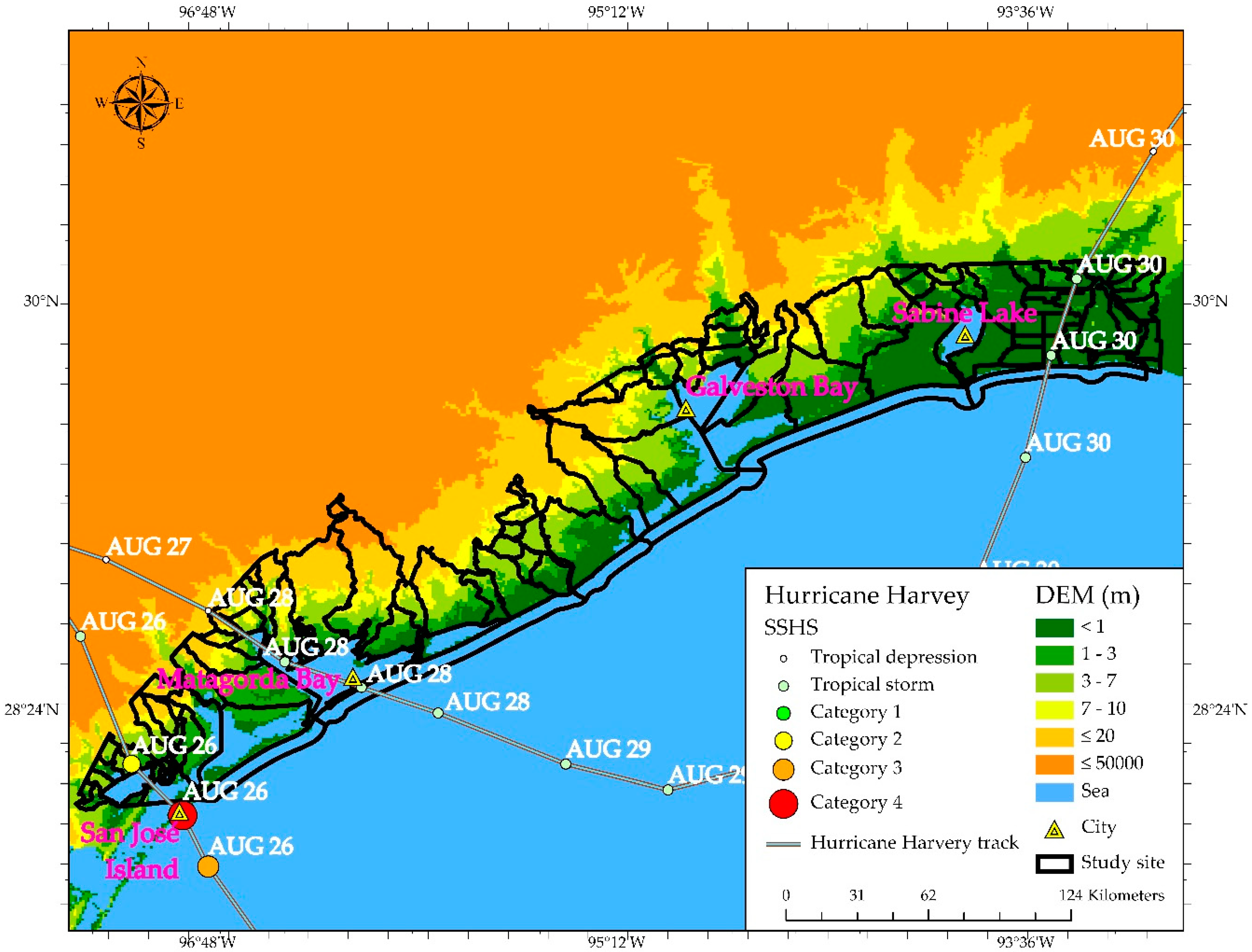
2.1. A Case Study: Hurricane Harvey

After Hurricane Katrina, the catastrophic effect of Hurricane Harvey is one of the costliest natural disasters in the United States [6]. Hurricane Harvey initially developed from a tropical wave to the east of the Lesser Antilles and became a tropical storm on 17 August, 2017. On 19 August, the storm weakened and degenerated into a tropical wave only to redevelop and intensify into a hurricane between 23 and 24 August [56]. Harvey eventually became a major hurricane and attained Category 4 intensity on 26 August. Three hours later, it made landfall at San José Island, Texas, at peak intensity (NHC, 2017). The path of Harvey’s center is represented by a cyan line in Figure 2. The proportional dot symbols with labels indicate the maximum sustained wind speeds. Flooding occurred in the study area along the South Texas Coast. According to Eric et al. [57], inundation from surge and tides was 6–10 feet above ground north and east of the landfall locations. Runoff from Harvey’s record-breaking rainfall, which exceeded 60 inches in some locations, also affected peak water levels. The total loss attributed to the storm at the time of landfall and the resultant consequences from flood disasters reached $125 billion, with more than 300,000 structures and 500,000 vehicles destroyed in Texas [6,57]. Sixty-eight people died as a direct consequence of Hurricane Harvey, with 65 of these due to freshwater flooding. More than 336,000 people were displaced from their homes and residences [57,58]. To assess the flood associated with Harvey, we focused on an area consisting of the sub-watershed basins clipped by coastal zone polygons developed for 2009. Almost all the basins are located in low elevation areas, making them extremely vulnerable to hurricane-induced storm surges and flash floods. When Harvey made landfall it triggered a flood in the study area of approximately 14,000 km² along the South Texas Coast. After making landfall at San José Island, Texas, Harvey exited from the center of Matagorda Bay (Figure 2).

2.2. Data Collection

The ATMS-SDR records are the primary dataset and were obtained from NOAA (https://www.avl.class.noaa.gov/saa/products/search?datatype_family=ATMS_SDR). The dataset was recorded on the National Polar-orbiting Operational Environmental Satellite System (NPOESS) which was a part of the NPOESS Preparatory Program (NPP) that began in 2006. It is the latest generation of cross-track microwave sounder providing atmospheric temperature and moisture for operational weather and climate applications [60]. Like the long heritage of its preprocessors, ATMS combines all of the channels of the preceding AMSU-A1, AMSU-A2, and AMSU-B sensors into a single package with considerable savings in mass, power, volume, and improved spatial resolution. Twenty-two channels in bands ranging from 23 GHz to 183 GHz are included (

Table 1. Channel characteristics of Advanced Technology Microwave Sounder (ATMS).

Channel	Frequency (GHz)	Quasi Polarization	Atmospheric Contribution (%)
1	23.8	QV	0.11
2	31.4	QV	0.06
3	50.3	QH	0.35
4	51.76	QH	0.51
5	52.8	QH	0.72
6	53.596 ± 0.115	QH	0.89
7	54.4	QH	0.97
8	54.94	QH	0.98
9	55.5	QH	0.99
10	57.29	QH	0.99
11	57.29 ± 0.217	QH	0.99
12	57.29 ± 0.322 ± 0.048	QH	0.99
13	57.29 ± 0.322 ± 0.022	QH	1.00
14	57.29 ± 0.322 ± 0.010	QH	1.00
15	57.29 ± 0.322 ± 0.0045	QH	1.00
16	88.2	QV	0.18
17	165.5	QH	0.58
18	183.31 ± 7.0	QH	0.94
19	183.31 ± 4.5	QH	0.98
20	183.31 ± 3.0	QH	0.99
21	183.31 ± 1.8	QH	0.99
22	183.31 ± 1.0	QH	0.99

). In this study, we chose channels 1, 3, 4, and 16 for estimating the large-scale coastal floods before and after Harvey made landfall. Brightness temperature values in each channel were extracted from ATMS Sensor Data Record (SDR) and converted into a raster file with a spatial resolution of 15 km using ArcGIS conversion tool. The near-nadir point ATMS records on August 18–19, 23, and 30 were collected before Harvey landfall and September 3 after Harvey landfall. To avoid image distortion, the satellite zenith angle extracted from these ATMS SDR files was limited to be smaller than 200. Aside from the ATMS data, DEM from Elevation Products (3DEP) at 1/3 arc-second resolution as distributed by Global Data Explorer of U.S. Geological Survey (USGS) (https://gdex.cr.usgs.gov/gdex/) were also obtained. The DEM data were the foundation of the coastal flood map, which significantly impacts the quality of the DWF model and its integration accuracy. In addition to the ATMS and DEM datasets, some ancillary datasets were also included to improve the estimation of flood extent:

• Watershed boundary dataset (WBD) developed by USGS (https://water.usgs.gov/GIS/huc.html);
• Flood-reported high-water-marks (HWMs) collected by USGS;
• Storm Surge Hindcast (SSH) product created by Coastal Emergency Risks Assessment (CERA);
• Coastal zone shapefiles 2009 from Data.gov (https://catalog.data.gov/dataset/shapefile-for-coastal-zone-management-program-counties-of-the-united-states-and-its-territories).
• 100 m National Land Cover Database 2006 from USGS. (https://viewer.nationalmap.gov/basic/?category=nlcd).

In this study, WBD data and Landcover database were used to identify land and water samples and downscale coarse-resolution flood maps. WBD consists of a series of Hydrologic Units (HUs) based on a hierarchical system of nesting hydrological units at various scales with a designation of unit codes—HU2, HU4, HU6, HU8, etc. [61]. In terms of the study site and ATMS spatial resolution, WBD HU12—that captures tributary systems—at sub-watershed level was selected as basin boundary. Based on the WF distribution, 108 sub-watershed basins were classified into five big regions for further quantitative analysis to assess flood dynamics comprehensively. The coastal zones are collected to identify these coastal basins for DEM-based downscaling analysis. A coupled model, the Advanced Circulation (ADCIRC) model, and Simulating Waves Nearshore (SWAN) model has been used to create CERA SSH products—used for DWF accuracy assessment. The ADCIRC model evaluates wind data spatially in different periods and calculates sea levels and currents. The original wind data and water level data are then proceeded to the SWAN model to simulate the wave actions [62]. This coupled model performs well with the storm-tide observation and wave actions during Hurricane Sandy [63] and has been adopted for Harvey. Another validation process compared the DWF map developed in this paper with HWMs. The HWMs are recorded by USGS representing the maximum rise of a body of water over land [58]. Here, we collected flood-reported HWM records from USGS (https://stn.wim.usgs.gov/fev/#HarveyAug2017) along the South Texas coastline, from San José Island to Sabine Lake, to evaluate the DWF flood map produced in this study.

2.3. Preprocessing

In this study, the brightness temperature (BT) value $\left(T\right)$ is utilized to create water fraction maps. Typically, $T$ can be represented as

$$T=T_{raw}·T_f$$

(1)

where $T_{raw}$ is the raw data of brightness temperature and $T_f$ is the brightness temperature factor. These two parameters were derived from ATMS SDR files. After calculating the brightness temperature values, ATMS channel records were resampled to 15 km using ArcGIS resample tool. Generally, longer wavelength passive microwave has the capacity to penetrate clouds. However, shorter wavelengths cannot be completely free of clouds due to the negative influence of atmospheric environments. In this case, a cloud detection process was necessary to remove possible cloud cover effects before extracting land surface information. A pixel in the ATMS raster is defined as a cloud pixel if Equation (2) is met [64]

$$T_{16}-T_1\ge 60 K$$

(2)

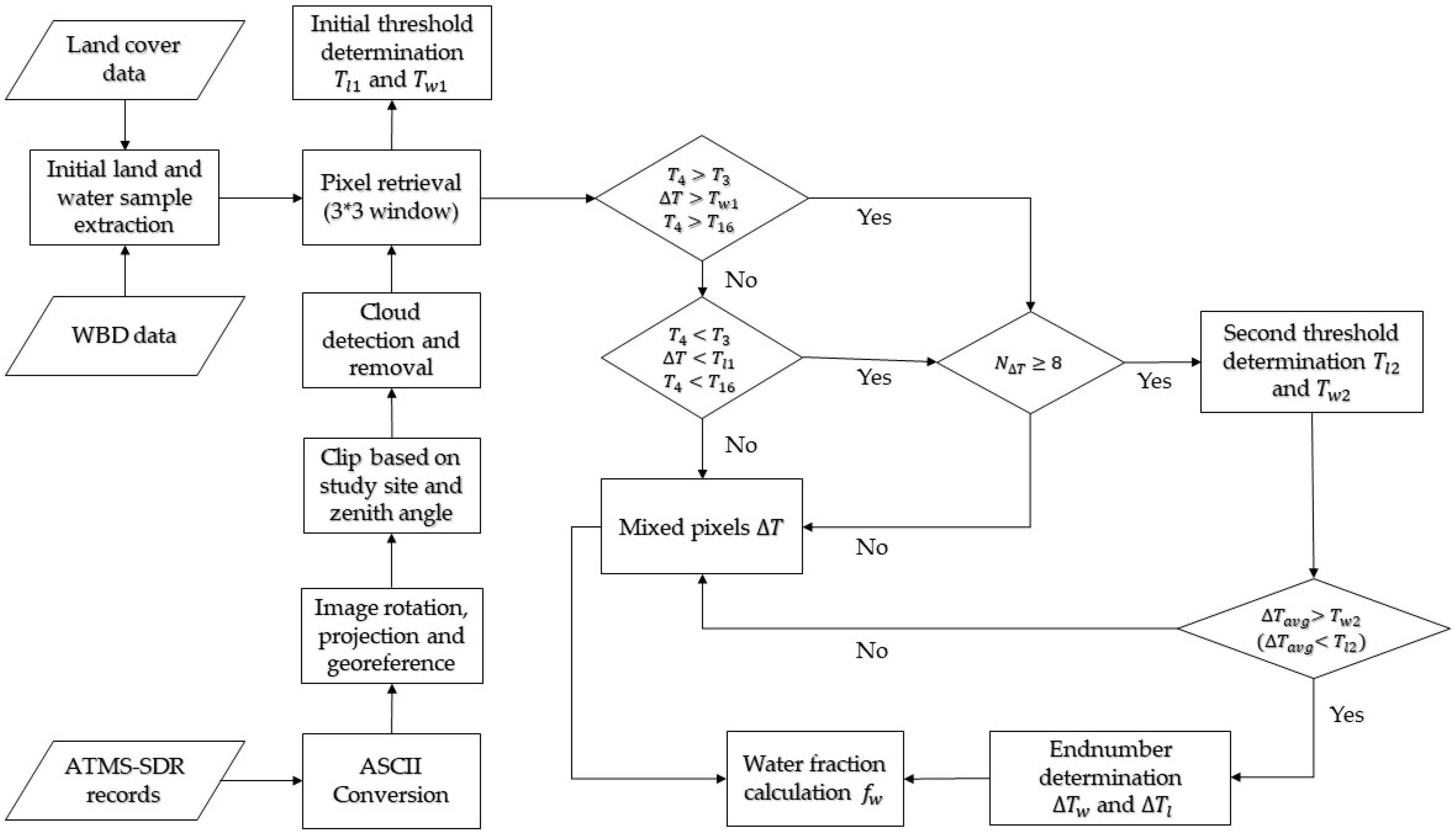
2.4. Water Fraction Model

A water fraction model was used to calculate the percentage of water extent for each ATMS pixel based on ATMS channel characteristics. Based on previous studies, ATMS channels 1–4 (Table 1) are all near the atmospheric absorption window and have a more significant contribution to the Earth’s surface radiance despite the impact of precipitation clouds [65]. Furthermore, because channel 3–4 have longer wavelengths and similar atmospheric absorption, the horizontally polarized difference of brightness temperatures between them is widely used to distinguish water and land features by minimizing atmospheric disturbances [32]. After analyzing the brightness temperature of water and land samples derived from WBD and linear hydrographic data, we found that the BT values of land samples and water samples in channel 3–4 & 16 follow the equations as follows,

$$T_{4_l}<T_{3_l}<T_{{16}_l}$$

(3)

$$T_{4_w}>T_{{16}_w}>T_{3_w}$$

(4)

$$\Delta T_{{\left(4-3\right)}_w}>13.4$$

(5)

$$\Delta T_{{\left(4-3\right)}_l}<0$$

(6)

where $T_{3_l}, T_{4_l}, T_{{16}_l}$ represents BT values of channel 3–4 and channel 16 in land pixels, respectively; $T_{3_w}, T_{4_w}, T_{{16}_w}$ represents BT values of channel 3–4 and channel 16 in water pixels, respectively; and $\Delta T_{{\left(4-3\right)}_w}, \Delta T_{{\left(4-3\right)}_l}$ represents the BT difference between channel 3 and 4 of water samples and land samples.

In order to thoroughly examine the sensitivity of extracting land and water information from ATMS channel 3, 4 and 16, sample records captured on 18–19, 23, & 30 August and 3 September were selected. The exact BT values in channel 3–4 & 16 of land samples and water samples are displayed in Figure 3. The BT differences between channel 4 and 3 during the study time are displayed in Figure 4. From these two figures, it is obvious to see that the BT difference between channel 4 and 3 are distinguishable. For estimating fractional inundation area from ATMS mixed pixels, a linear mixed model with two pure feature factors has been developed by Sippel et al. [32,42] using the following equation,

$$\Delta T_{{\left(4-3\right)}_{mix}}=f_w·\Delta T_{{\left(4-3\right)}_w}+\left(1-f_w\right)\Delta T_{{\left(4-3\right)}_l}$$

(7)

where $\Delta T_{{\left(4-3\right)}_{mix}}$ is the BT difference observed by the radiometer and $f_w$ is the fractional water area.

From Equation (7), $f_w$ can be expressed as:

$$f_w=\frac{\Delta T_{{\left(4-3\right)}_{mix}}-\Delta T_{{\left(4-3\right)}_l}}{\Delta T_{{\left(4-3\right)}_w}-\Delta T_{{\left(4-3\right)}_l}}$$

(8)

The water fraction value $f_w$ was extracted by applying the dynamical mechanism using MATLAB and Python (Supplementary Materials). To identify $\Delta T_{{\left(4-3\right)}_w}$ and $\Delta T_{{\left(4-3\right)}_l}$, Equations (3) to (6) were empirically used to distinguish initial water threshold $T_{w1}$ and initial land threshold $T_{l1}$ based on sub-watershed basins as well as landcover data. All pixels in the AMTS imagery were looped. For those pixel $\Delta T_{{\left(4-3\right)}_{mix}}$ whose 3 × 3 neighborhood pixels are all greater than $T_{w1}$ or smaller than $T_{l1}$, an average calculation will be assigned and this average value $\Delta T_{{\left(4-3\right)}_{avg\_mix}}$ will be identified as either pure water threshold $T_{w2}$ or pure land threshold $T_{l2}$. Then, for each $\Delta T_{{\left(4-3\right)}_{avg\_mix}}$ pixel, the average of its 3 × 3 neighborhood pixels bigger than $T_{w2}$ or smaller than $T_{l2}$ will be assigned as $\Delta T_{{\left(4-3\right)}_w}$ or $\Delta T_{{\left(4-3\right)}_l}$. Finally, based on Equation (8), the water fraction values can be extracted using $\Delta T_{{\left(4-3\right)}_w}$, $\Delta T_{{\left(4-3\right)}_l}$ as well as $\Delta T_{{\left(4-3\right)}_{mix}}$.

2.5. DEM-Based Water Fraction (DWF) Map Derived from DEM-Based Downscaling Model

The water fraction value extracted is a mix of many kinds of surface features like water, soil, and vegetation, which is challenging to differentiate and estimate their factor variables using ATMS data [66]. In this case, a water fraction extent comparison before and after Hurricane Harvey’s landfall is necessary to remove the negative impacts exerted from these factors [67]. The calculation of water fraction extent comparison is

$$f_{w_a}-f_{w_b}=A_{Flood}$$

(9)

where $f_{w_a}$ is the average water fraction after Hurricane Harvey, $f_{w_b}$ is the average water fraction before Hurricane Harvey and $A_{Flood}$ is the inundated area.

The flooded area derived from ATMS data has a 15 km spatial resolution, which is too coarse to estimate the flood extent accurately. To solve this problem, an integrated method combining basin-scale water properties and DEM-based inundation mechanism was introduced [43]. This inundation mechanism can be expressed as

$$A_{Basin\_flood}={{\displaystyle \int }}_{mi{n}_h}^{ma{x}_h}f\left(h\right)dh$$

(10)

where $A_{Basin\_flood}$ is the flooded area in a specific basin, $ma{x}_h$ and $mi{n}_h$ are the maximum flood elevation and DEM-based value, $f\left(h\right)$ is the increment of water area with the increase of water surface elevation $h$ in a basin.

Equation (10) can be explained as follows; as the earth’s surface near the coast is gradually inundated by storm surge, its elevation will start to increase from the $mi{n}_h$. When the inundated water surface area percentage equals to the water fraction, the increase in water elevation will stop when it approaches the maximum water elevation $ma{x}_h$. After this process, all the DEM pixels in a specific basin whose elevation value changed will be assigned as pure water cells. In Equation (10), $mi{n}_h$ can be directly derived from 10 m DEM data. $A_{Flood}$ can also be determined after calculating the water fraction difference using Equation (9). Based on the inundation mechanism, water fraction estimates can be transformed into high-resolution flood maps which have the same spatial resolution as DEM sources. Finally, the DWF map was generated based on water faction model and DEM-based downscaling model.

2.6. DWF Flood Map Validation

CERA SSH product was used as a benchmark for DWF map validation. The product was downloaded from the National Weather Service distributed by NOAA (https://cera.coastalrisk.live/). To evaluate the quality of the DWF flood map, the CERA SSH product was overlapped with DWF flood map. The comparison between these two maps was performed pixel-by-pixel using 15 km $\times$ 15 km grids along the flooded coast.

Aside from the CERA SSH product validation process, we used flood-reported HWMs to validate DWF result for a further accuracy assessment. The specific locations of flood-reported HWMs are shown in Figure 10, which were used to overlay the DWF flood map. Considering the geolocation error and different spatial resolution, the HWM points were all buffered to 200 m. Buffered zones that intersected with DWF flood map were selected as DWF-determined HWM buffered zones. Similarly, we applied the same process to CERA SSH product using HWMs and identified CERA SSH-determined HWM buffered zones. The comparison between the DWF and CERA SSH maps with the use of the HWMs are listed in

Table 2. Quantitative comparative analysis of DWF map and CERA SSH product.

No	DWF		Non-DWF		CERA SSH		Non-CERA SSH
	Area (ha) Area (%)	HWMs HWMs (%)	Area (ha) Area (%)	HWMs HWMs (%)	Area (ha) Area (%)	HWMs HWMs (%)	Area (ha) Area (%)	HWMs HWMs (%)
1	74,989 27.40%	37 97.37%	198,725 72.60%	1 2.63%	71,661 26.18%	37 97.37%	202,053 73.82%	1 2.63%
2	301,495 75.69%	51 100%	96,833 24.31%	0 0%	279,220 70.10%	47 92.16%	119,108 29.90%	4 7.84%
3	178,437 27.55%	61 85.92%	438,160 72.45%	10 14.08%	110,532 17.93%	52 73.24%	506,065 82.07%	19 26.76%
4	241,514 49.73%	31 100%	223,731 50.27%	0 0%	189,626 40.76%	26 83.87%	275,619 59.24%	5 16.13%
5	349,091 44.68%	4 100%	422,012 55.32%	0 0%	392,413 50.89%	4 100%	378,690 49.11%	0 0%

Note—‘No’ represents the five classified regions after generating WF difference map. ‘Area (ha)’ and ‘Area (%)’ refer to the flood area in each region and its corresponding flood portion, respectively. ‘HWMs’ and ‘HWMs (%)’ refers to the count of HWM buffer zones overlapping with DWF map and/or CERA SSH product, respectively.

.

3. Results

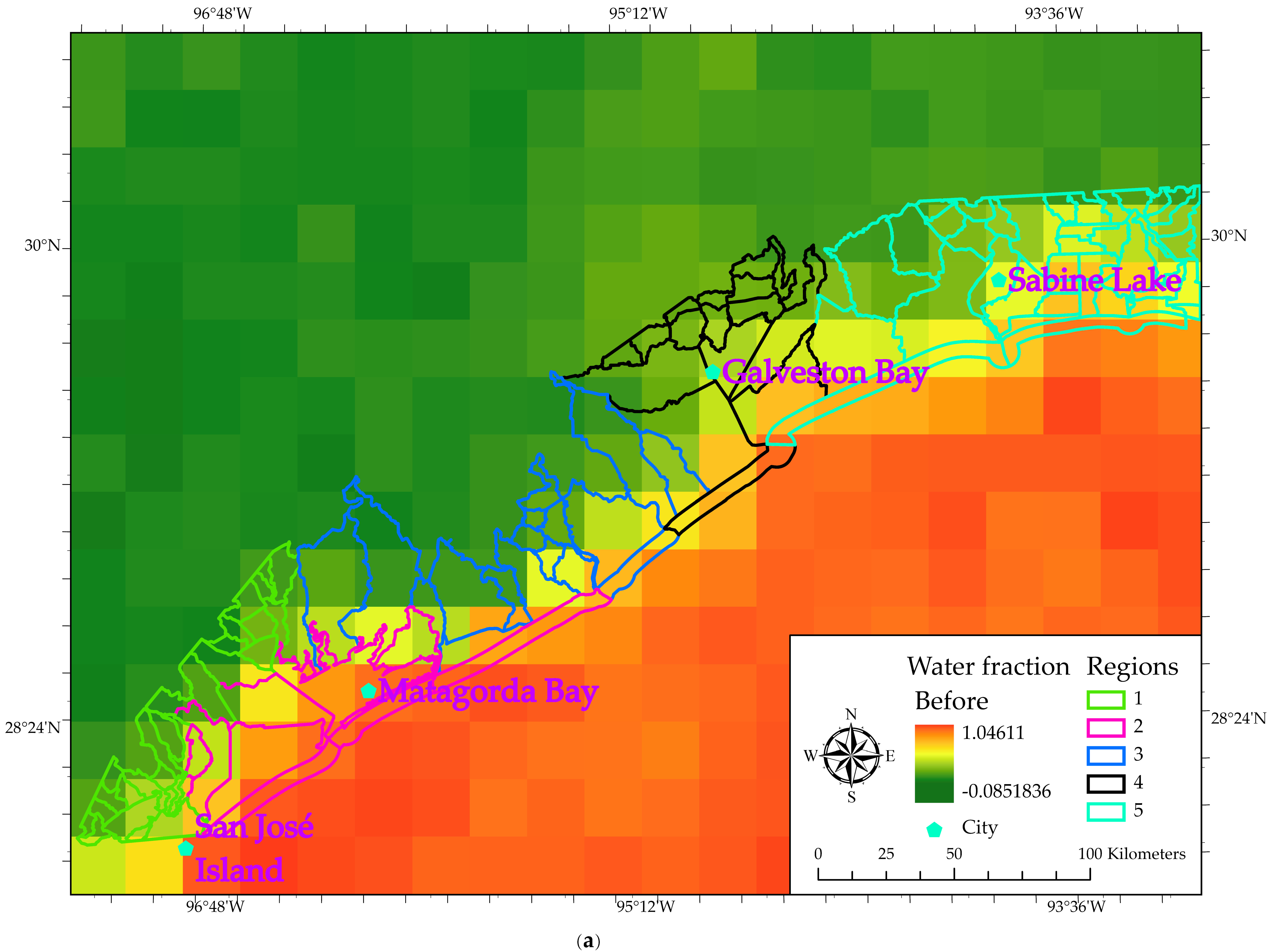
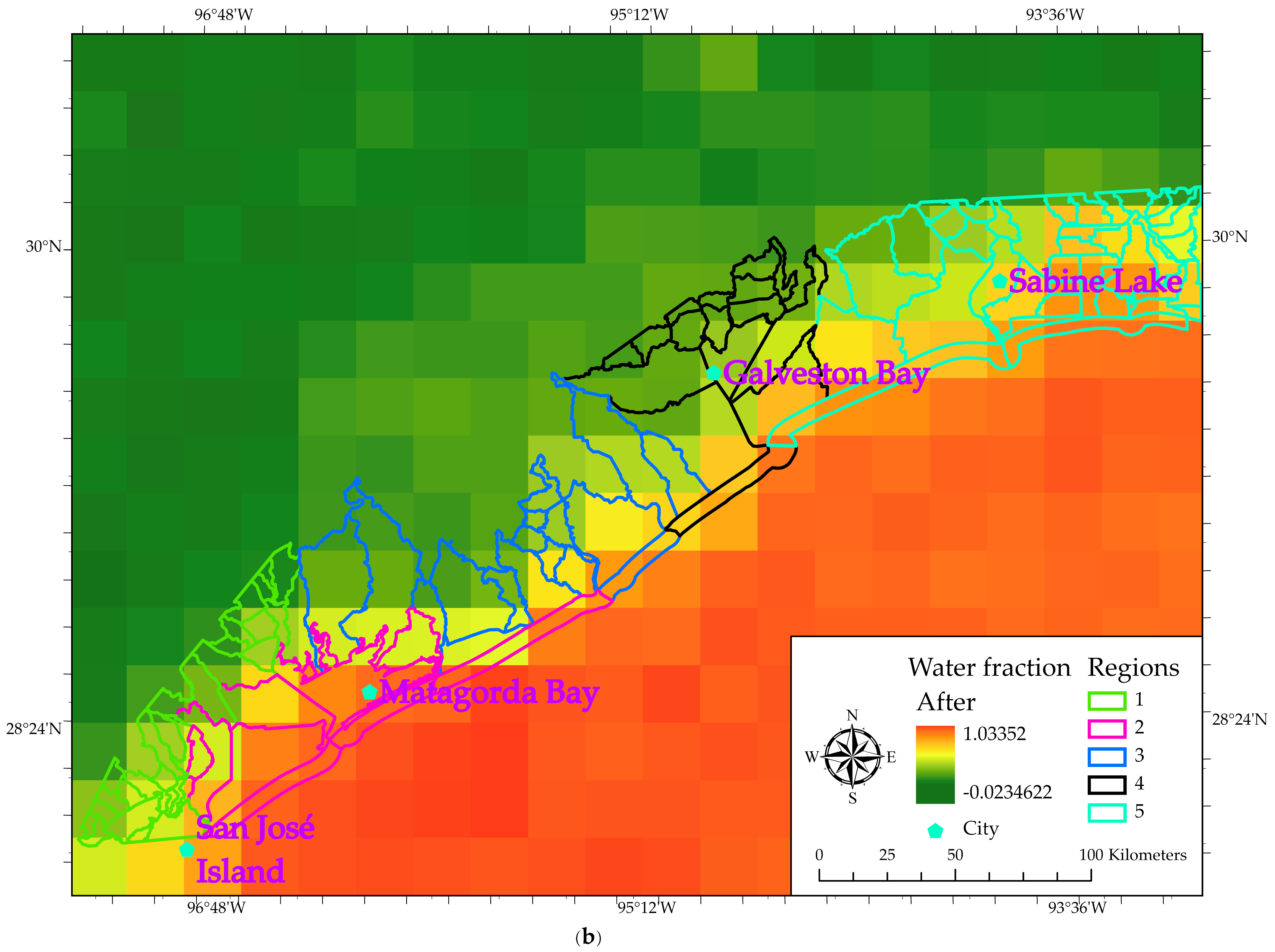
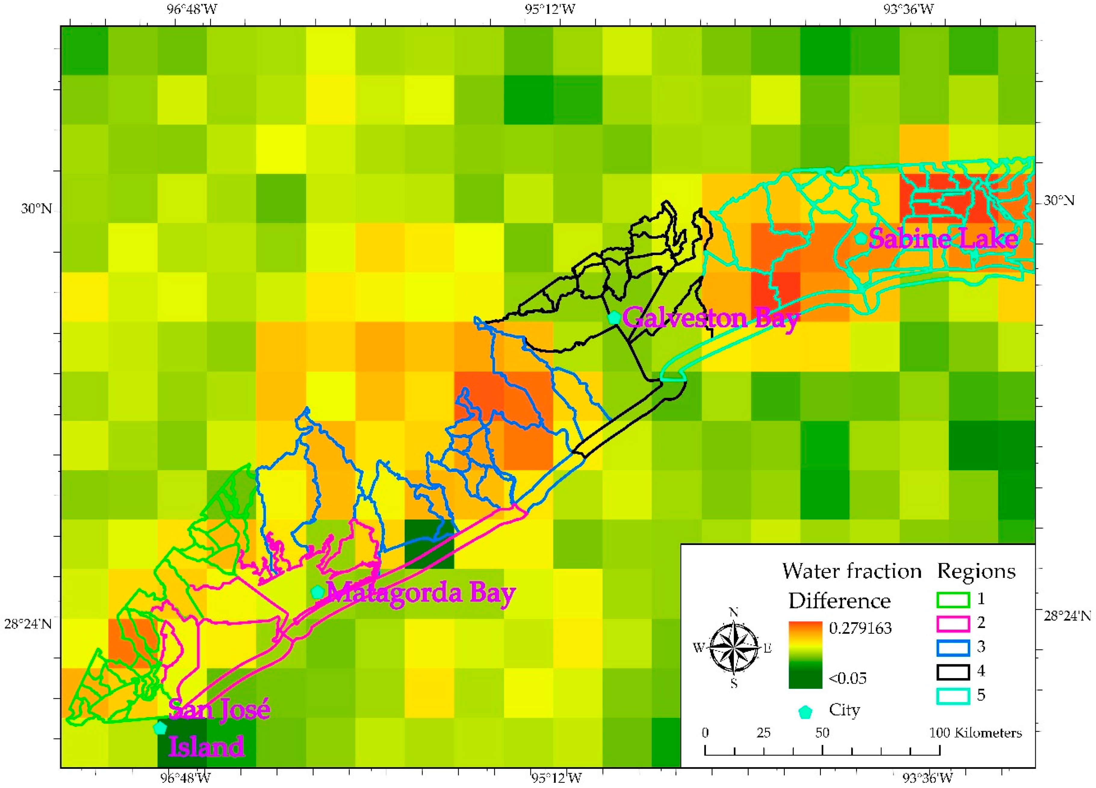
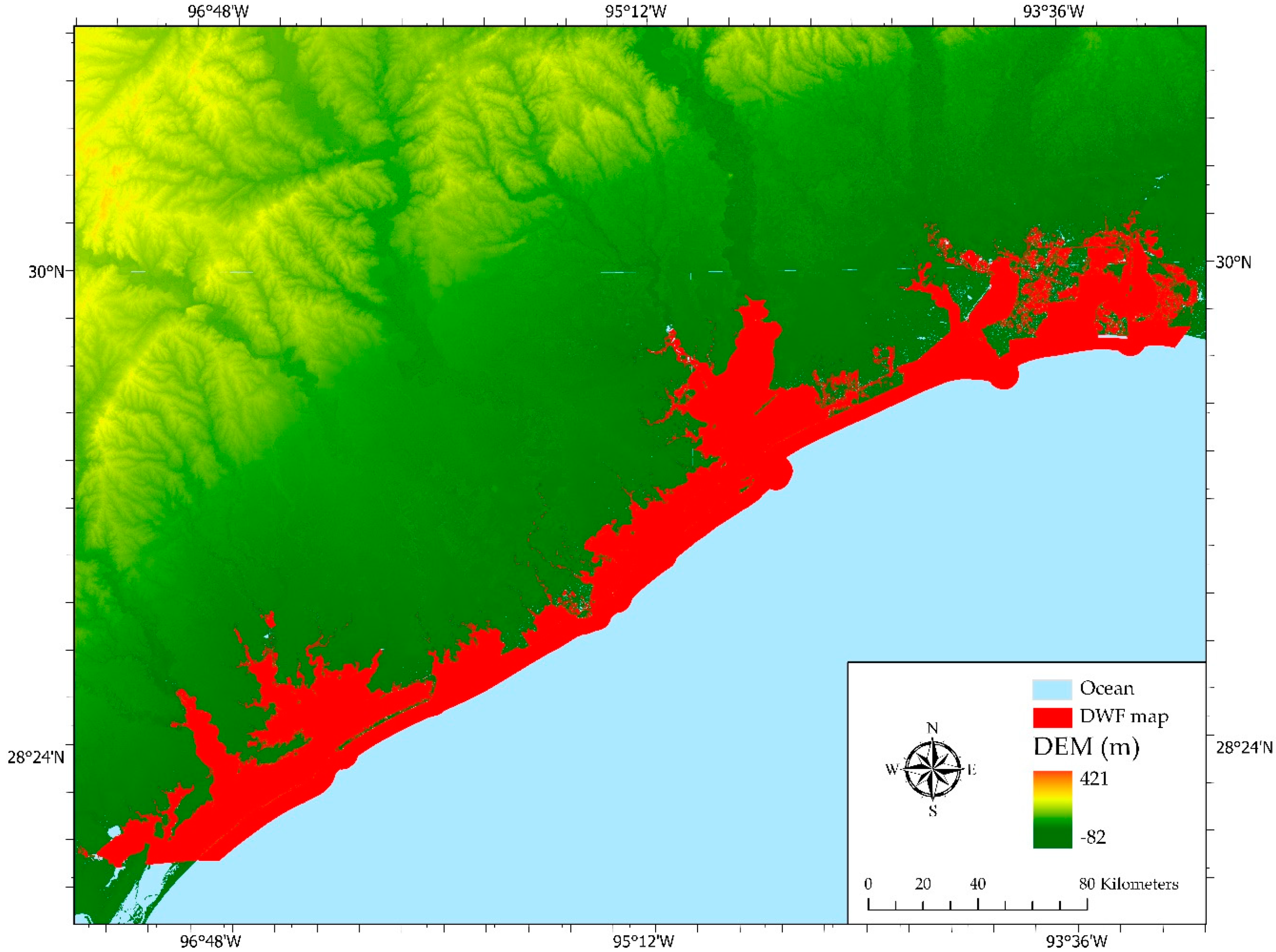
3.1. DEM-Based WF (DWF) Map

The water fraction model demonstrates the feasibility of estimating large-scale flood extent. The results of the average WF map (Figure 5) show the spatial distribution of WF values before Hurricane Harvey’s landfall (Figure 5a) and after Hurricane Harvey landfall (Figure 5b). Land-dominated pixels appear deeper in green color while water-dominated pixels appear deeper in red color. In order to visualize the spatial extent of flooded areas, a subtraction operation was applied to these two WF maps, such that the pre-hurricane WF map was subtracted by the post-hurricane WF map (Figure 6). Previous studies demonstrated that a WF value of 0.05 better matches with flood pixels [68]. In the WF difference map, most of the positive WF values greater than 0.05 are clustered near the north of San José Island, coastal areas between Matagorda Bay and Galveston Bay, and most regions around Sabine Lake. Regions 1 and 2 contain moderate WF value (0.1 < WF < 0.2) basins; regions 3 and 5 have high WF value (WF > 0.2) basins; most coastal basins have low WF values (WF < 0.1) in region 4. Although WF pixels in region 4 have relatively low values, they are still regarded as flood-determined pixels because their values are greater than 0.05. In order to quantitatively compare the WF values before and after Hurricane Harvey made landfall, an independent sample t-Test was conducted. The result reveals that the post-hurricane WF values are significantly different compared with the pre-hurricane WF values with a p-value of 0.01 (Appendix A). It therefore implies that the post-hurricane WF values after Hurricane Harvey increased significantly compared with the pre-hurricane WF values.

Even though the spatial pattern of flooded areas can be roughly derived from the WF difference map, it is still impossible to estimate the flood extent accurately based on the WF difference map whose pixel size is coarse at 15 km. For the sake of high-resolution flood estimation, a DEM-based downscaling model was performed to improve the spatial resolution of the WF difference map based on topographic information and hydrologic mechanisms. Specifically, 10 m DEM raster data clipped by the study site were converted to points with the same cell size. These DEM points were then grouped by 108 sub-watershed basins. Flood-determined DEM points for each basin were generated based on hydrologic mechanisms discussed in Section 2.5. Finally, these flood-determined DEM points were converted to multiple raster and polygon datasets for high-resolution flood visualization and accuracy assessment. Figure 7 shows the result of the developed 10 m DWF map where the flood extent can be easily observed along the long coastline in South Texas. The DWF map also demonstrates high suitability of estimating large-scale inundation areas using ATMS and DEM dataset.

3.2. Accuracy Assessment

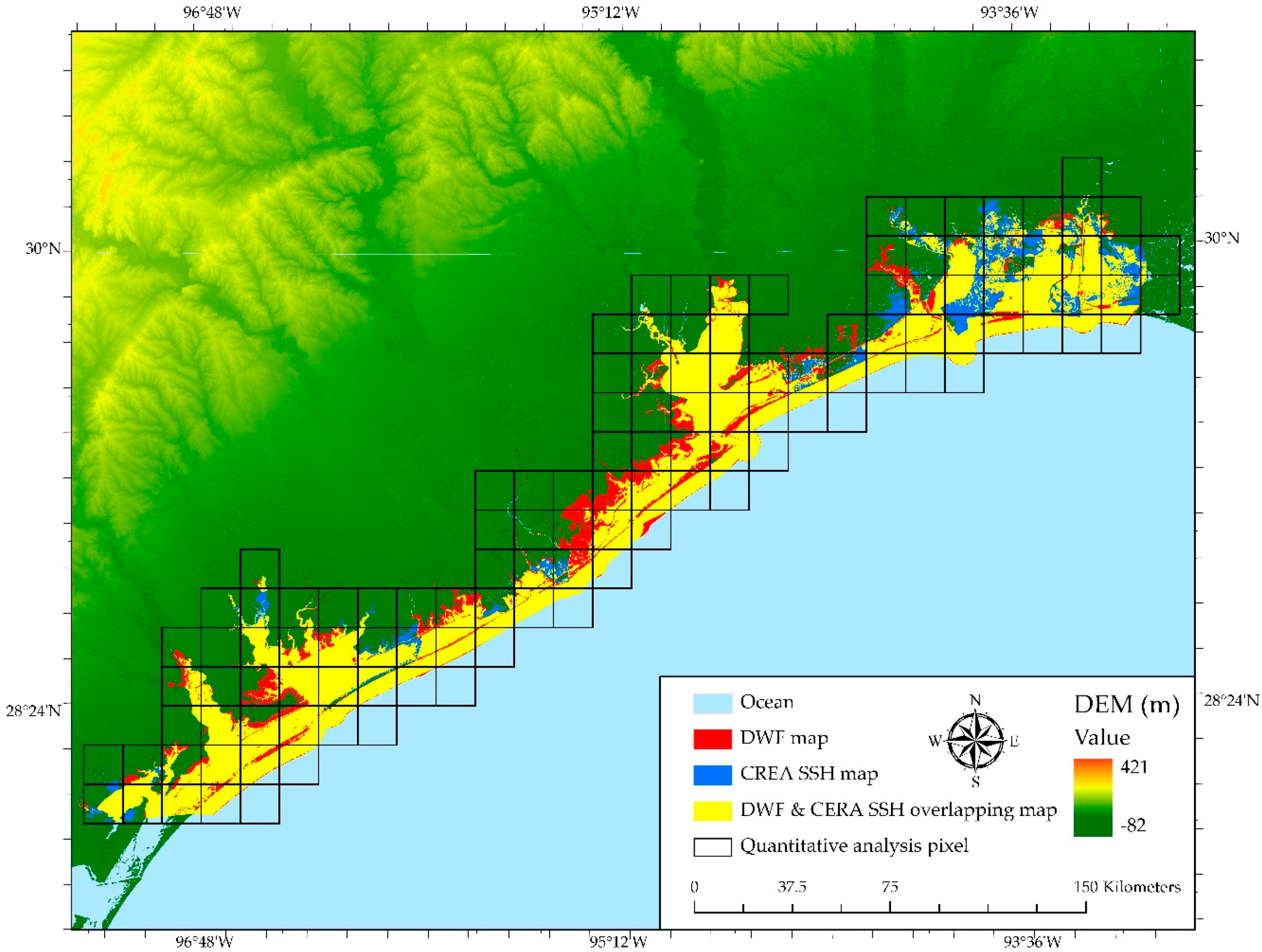
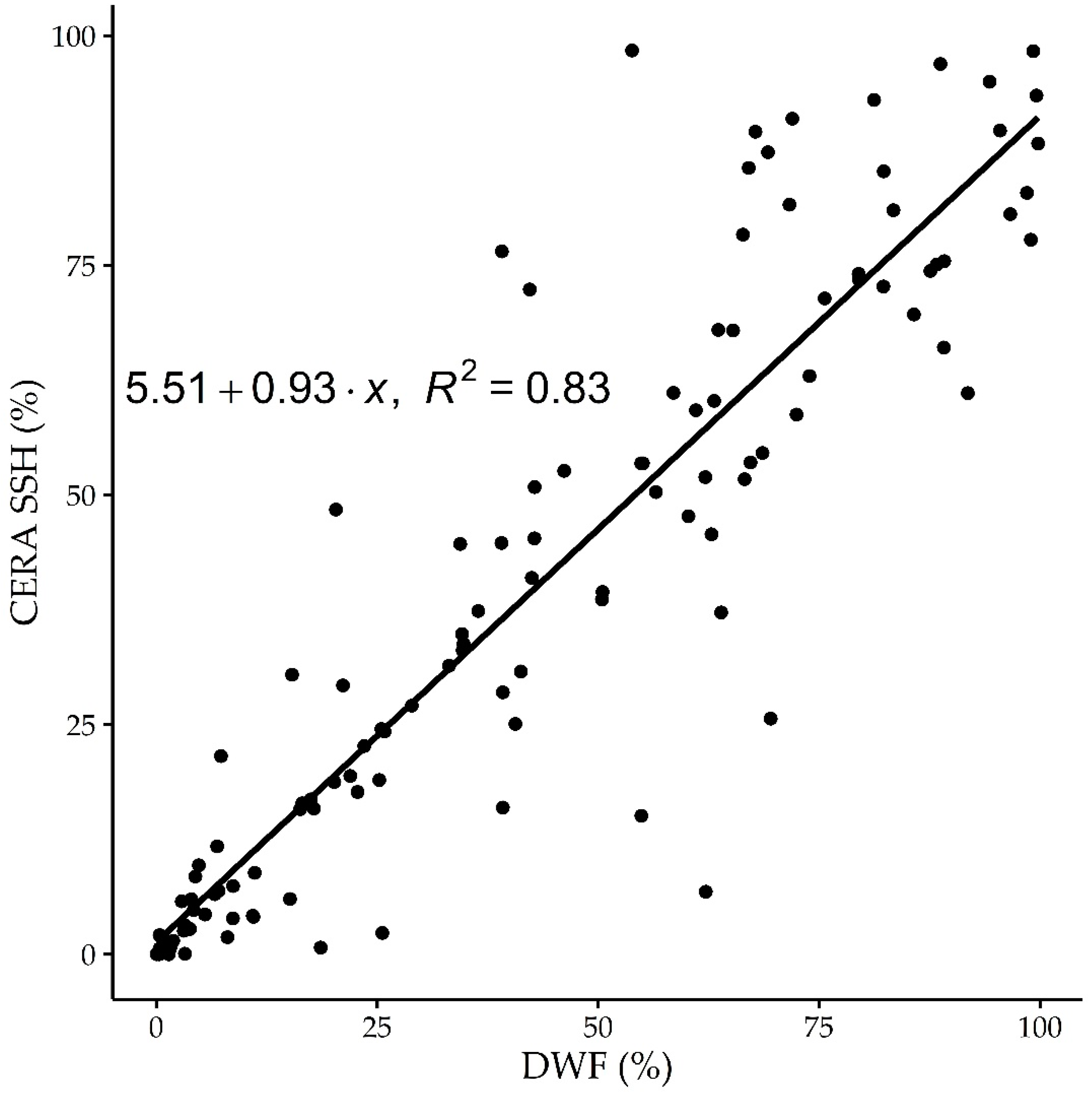
3.2.1. Comparison with CERA SSH Product

For the detection of coastal flood differences between the DWF map and the CERA SSH product, zonal change detection method was applied [69]. The differences between the DWF and CERA SSH maps showed a high level of similarity (Figure 8). The DWF-determined flooded areas appear in red, CERA SSH-determined flooded areas are blue, and overlapping areas were assigned yellow. It is evident to that regions 1 and 2 in Southwestern Texas Coast have many overlapping areas. More DWF-determined flooded areas are clustered in regions 3 and 4, while more CERA SSH-determined flooded areas are clustered in region 5. To quantitatively compare these two maps, one hundred and twenty three (123) 15 km $\times$ 15 km grids were generated to cover all coastal basins For both DWF and CERA SSH maps, we calculated the percentage of inundation areas in each grid and applied a zonal statistics function to spatially examine the similarity—a method also applied by Elsner et al. [70]. It was found that the spatial extents of DWF map, CERA SSH product, and their overlapping map are 121,355, 199,830 and 923,015 hectares, respectively, accounting for 4.38%, 7.22% and 33.35% of the total area. The overlapping areas are attributed to 74.19% of the total areas occupied by water. A good linear relationship was observed between percentages of inundation areas in both DWF and CERA SSH maps with a Pearson’s correlation of 0.91 and an R-square of 0.83 (see Figure 9). To examine the spatial distribution of flooded areas in these two maps, the flooded area and corresponding area percentage of DWF and CERA SSH maps, in each region, were derived (Table 2). These regions are used to quantify the spatial similarity and dissimilarity of DWF and CERA SSH maps [71]. Region 1 has the smallest DWF flooded area of 27.4% of the total area and smallest CERA SSH flooded area of 26.18%. Whereas, region 5 has the largest DWF flooded area of 45.27% of the total area and the largest CERA SSH flooded area of 50.89%. There is a slight difference between DWF and CERA SSH maps in region 1 with a percentage of approximately 1. The flood percentage of DWF map is 5.59% greater in region 2 and 6.21% smaller in region 5 than that of CERA SSH map. While in region 3–4, the percentages of DWF-determined flooded areas are around 10% greater than that of CERA SSH-determined flooded areas. To find out if the flooded areas in DWF map are overestimated or not in regard to CERA SSH product, further accuracy assessment was implemented.

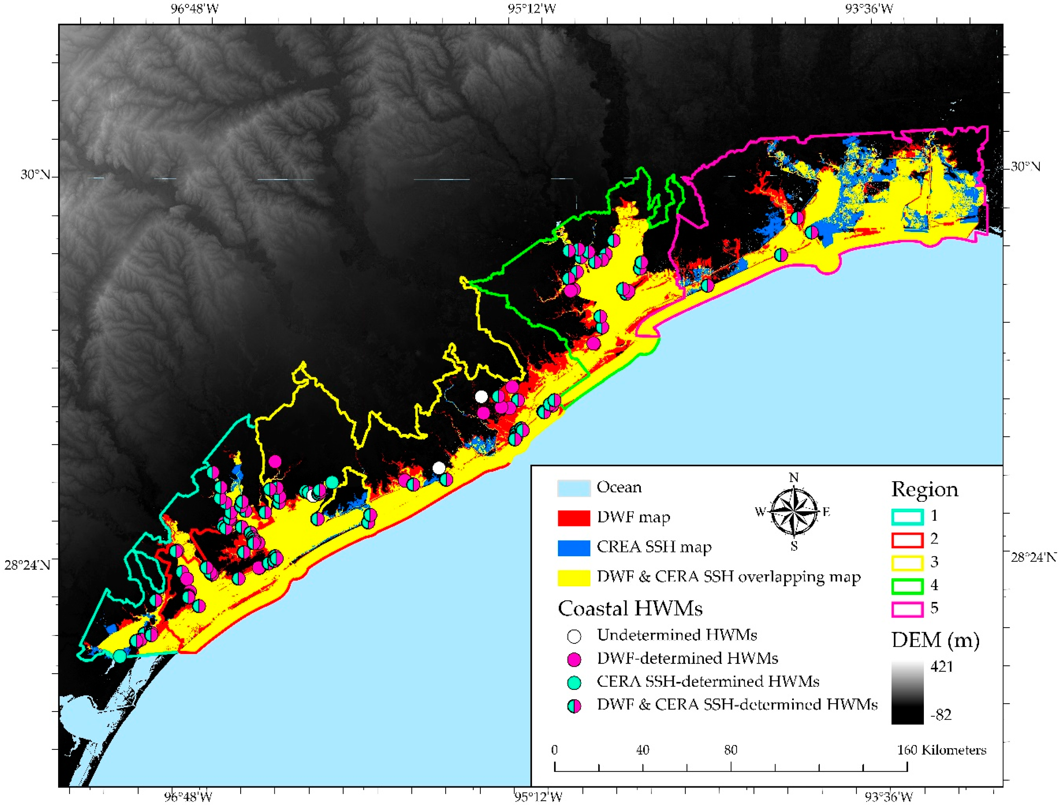
3.2.2. Quantitative Assessment Using HWMs

After comparing the DWF map with the SERA SSH product, we can conclude that the DWF flood map has a relatively high agreement with the SSH product. However, some differences between these maps were found in region 2–5 (Figure 8). To further compare DWF and CERA SSH maps, the real-time HWMs were used in the validation process. The coastal HWMs that were identified as a field- verified HWMs during Hurricane Harvey were selected to evaluate DWF map and CERA SSH product. These data were collected and verified by USGS and NOAA. The spatial distribution of 195 coastal HWMs is shown in Figure 10. HWMs were buffered to 200 m circle zones to reduce geographic errors. Undetermined HWMs represent those buffered HWMs without an intersect with either DWF map or CERA SSH product. DWF-determined HWMs represent those buffered HWMs intersecting with DWF map. CERA SSH-determined HWMs represent those buffered HWMs who intersect with only CERA SSH product. DWF & CERA SSH-determined HWMs represent buffered HWMs who intersect with both DWF map and CERA SSH product. Overall, DWF map has covered 184 out of 195 (94.36%) buffered HWMs; CERA SSH product has covered 166 out of 195 (85.12%). Specifically, the coastal HWM counts and corresponding percentage information are shown in Table 2. It is obvious that DWF map has overlapped more buffered HWM zones than CERA SSH in five regions. In region 1–2, the percentage of overlapped HWMs in both maps are over 90%. In region 3–4, more HWM buffered zones have intersected with DWF maps rather than CERA SSH product. With regards to region 5, even though the DWF flooded area is 5.62% smaller than that of CERA SSH flooded area—both maps have overlapped with the same number of HWM buffered zones in region 5. We can conclude that DWF-determined flooded areas in region 3–5 fit significantly with the HWMs. The result of quantitative assessment also indicates that DWF map has a higher consistency with HWMs compared with CERA SSH product.

4. Discussion

4.1. Main Findings

This study has successfully implemented the DWF method to estimate the large-scale extent of coastal floods induced by Hurricane Harvey in a higher spatial resolution than previously accomplished. A three-step process was conducted to calculate water fraction values, and the coarse-resolution flood map was downscaled to a better resolution. The differences between the post-hurricane WF values and pre-hurricane WF values, as shown in the T-test, was as a result of the hurricane making landfall and carrying heavy precipitation along with it. The downscaled WF (DWF) was then validated using CERA SSH product and flood-reported HWMs. The result shows that the linear relationship between the DWF map and CERA SSH product is statistically significant with a p-value smaller than 0.05, a correlation coefficient of 0.91 and an R-square of 0.83. Furthermore, the DWF map has also overlapped with more than 85% of the total flood-reported HWMs in all 5 regions demonstrating a good agreement between DWF map and HWMs. Some findings showing the availability and efficiency of proposed DWF method are as follows:

• The wide swath and daily temporal resolution of ATMS data in this research demonstrate an excellent capability of monitoring and mapping large-scale flood extent. Specifically, ATMS wide swath is big enough to cover the South Texas Coast using just one scene of ATMS image.
• ATMS sensors on the satellites are not usually affected by atmospheric constituents such as water vapor, dust, clouds, etc. [36]. In this case, ATMS data is free of cloud cover and dense vegetation to some extent and is widely used to measure land surface features in different weather within 24 h of measurement. However, high-frequency ATMS channels like the 3–4 channels used in this study cannot penetrate thick rain bands of hurricanes, which is why our study periods were selected before and after Hurricane Harvey passed over the region. Goldberg [72] used SNPP/VIIRS resolution and GOES-16 geostationary satellite data with resolutions of 375 m and 1 km respectively to monitor floods induced by Hurricane Harvey. Although these satellites have better resolution than the one applied, they cannot penetrate through cloud cover. This could create uncertainty in the result even though the use of GOES-16 dataset serves to partially reduce the influence of cloud cover. Also, the authors did not downscale the coarse satellite data using a DEM which was done in this study. It is therefore essential to downscale the satellite-derived flood maps. Brakenridge et al. [46], after studying Hurricane Katrina using satellite images like MODIS and Sea, Lake, and Overland Surges from Hurricanes (SLOSH), concluded that combining MODIS maps and DEMs from LiDAR will be helpful to increase the accuracy of estimating storm surge.
• The outcome of this study made it evident that the use of high-resolution DEM provides feasibility to develop high-resolution flood maps from downscaled passive microwave measurements. The results from the DWF illustrate that this method can integrate water surface estimates, elevation information, basin boundaries, and hydrological mechanism and develop a flood map relatively easier and faster with good quality for disaster response and recovery. Li [43], equally used MODIS 500 m water fraction map and then downscaled to the resolution of DEM-30. He argued that incorporating a low-resolution DEM into a model may greatly change the flow direction and accumulation of the water, resulting in an error when integrating the DEM data and the TEERA/MODIS derived water fraction. This procedure produces more accurate results when a finer resolution DEM is used as in the case of the current study. The vertical accuracy of the 30 m SRTM DEM, which is 6–8 m as reported by [73], used by [43] in their elevation model did cause a substantial difference, over a plane surface, in modeled inundation areas. Because of the finer resolution −10 m DEM—used in this research with a vertical accuracy of 3 m [74], the differences over plain sites are essentially minimal [64]. Furthermore, when [29] performed similar research for Hurricane Sandy, using 100 m resolution, they opined that the resolution of the DEM used cannot depict detailed information and errors may emerge within the created flood-map. Although the 10 m data used in this study does not imply that extremely detailed topographic information can be depicted with high accuracy, we assert that the errors have been greatly reduced as compared to what is obtainable in the research by Li et al. [43] and Zheng et al. [29] since the vertical accuracy for the DEM used here is better than that used in other improved basin-based methods.
• The study provided an improved basin-based method. During a hurricane event, there is usually a transfer of mass and energy in the water element, so much so, that the ocean body increases in water level resulting from the atmosphere and water body interaction [75]. These phenomena coincide with the tides and affect watersheds that are lying landward. The individual determination of catchment DWF (Table 2) reveal the exact extent to which the catchments were inundated. The study area was divided into regional sub-watersheds (Table 2) that were used as a unit of validation, resulting in better accuracy for individual basins. The results show the percentage of flooded and non-flooded zones for both DWF and CERA SSH models. It was necessary to downscale the ATMS data to the level of sub-watersheds as each area, represented here by the sub-watersheds has unique characteristics such as hydro-geomorphic, water volumes and anthropogenic influences. It was therefore expected that the flood from a hurricane would impact each sub-watershed differently because of their unique characteristics. Based on this scale we can observe the spatial differences of the impact of flood within the entire area. Furthermore, the use of sub-watershed units makes it easier to fit in the ATMS derived WF values when downscaling for improved accuracy.
• The sub-watershed basins grouped into five different regions (Table 2) examined the spatial distribution of similarity and dissimilarity of both DWF and CERA SSH flood maps. Using sub-watershed regions provided better accuracy for individual sub-watershed basins as spatial differences in the flood impacts were apparent. Therefore, we can conclude from the result, of the validation, that this technique is feasible for developing large scale flood analysis, especially when dividing the study area into multiple sub-watershed basins.

4.2. Limitations

Even though the DWF method has provided a good result, there are still some potential errors showing as follows,

• Zenith angle limitation and georeferencing problem: The pixel value in primary ATMS data appears to have a relatively low spatial resolution if the zenith angle is bigger than 20°. The cross-track and along-track FOV size of ATMS data range from 60 km to 136.7 km [65]. Therefore, it is nearly impossible to cover a large-scale study site with the best ATMS data near nadir. Furthermore, the AMTS sensor cannot capture the data at the same angle in the same place. In this case, georeferencing is highly recommended before water fraction values are calculated. A slight displacement in the georeferencing process will result in a critical negative impact on the quality of the DWF flood map.
• It is difficult to identify the factors that cause the uncertainty of $\Delta T_{{\left(4-3\right)}_{mix}}$: On the one hand, the large amount of rainfall falling on the South Texas Coast may vary in high temporal and spatial variability during Hurricane Harvey, which results in an even higher $\Delta T_{{\left(4-3\right)}_{mix}}$ by soil absorption and water accumulation. Vegetation may reduce the value of $\Delta T_{{\left(4-3\right)}_{mix}}$ greatly because soil moisture cannot be easily detected if soil features are covered by vegetation [76].
• Limitation of real-time datasets: Some regions in the DWF map, especially region 5, have substantial differences compared with CERA SSH product. The reason is that DWF used post-hurricane ATMS data collected before and after Hurricane Harvey dissipated on 3 September. The ATMS data are not available from when the coastal flooding was at its peak. In contrast, CERA SSH product was derived from ADCIRC model to estimate coastal flood extent using real-time observations, which is more likely to be accurate.
• DEM limitations: Even though 10 m 3DEP DEM dataset is good enough to downscale large-scale ATMS data, further study is needed to improve the resolution of elevation dataset because the DWF method presented relies on high-resolution elevation datasets. LiDAR data are an excellent choice due to their very high spatial resolution of less than 1 m with a vertical accuracy of less than 15 cm [77]. LiDAR data is also widely used to develop DSM and DTM elevation products for vegetation and building detection, which is even better to estimate flood extent in coastal urban areas [78]. Recent studies (e.g., [79]) also pointed out that as the DEM resolution becomes coarser, the estimated flood damages will be reduced. It would be better to quantify DEM data using ground control points if further risk assessments are needed.
• Neglect of other environmental factors: In this study, only topography information and passive microwave remote sensing images were considered for mapping coastal floods. However, coastal floods may become much more devastating due to other environmental factors like sea level rise (SLR), land subsidence (LS) and bathymetric change (BC). For instance, Wang et al. [80] applied MIKE 21, a flood simulation model, to estimate the flood intensity based on these three environmental factors. They found that BC is the main factor responsible for severe coastal floods while SLR and LS may affect more on coastal floods in the future due to climate change and urban development.

4.3. Coastal Flood Map: Communicating Risk

The flood risk management effort is usually necessary after large scale flooding to reduce socio-economic losses. Owing to the increasing impacts of climate change, more people are likely to be affected by coastal floods unless measures are put in place to reduce such impacts. Traditionally, flood risk management focussed predominantly on structural measures, the planning and implementation of which, for the most part, are the responsibilities of governments [2]. Flood risk management efforts in US cities are mainly completed by the Federal Emergency Management Agency (FEMA) in collaboration with other organizations. As part of the process of flood management, government agencies need to move, very rapidly, away from cartography-oriented risk management. A framework that embodies risk communication to a layman should be firmly adopted. After mapping large-scale coastal floods such as conducted here, our work offers an opportunity for effective communication to stakeholders, practitioners, and policymakers, a crucial element of flood management [81] to increase risk awareness and flood preparedness. The DWF map developed in this study can be adopted to any coastal flood situation as it has the potential to be reproduced rapidly after a flood event. The resultant map can be used as a tool for risk communication through interactive visualization, for example through an online map running an algorithm on a major government website such as FEMA.gov. Olsen et al. [82] proposed a state-of-the-art approach, using realistic interactive visualization to improve flood risk communication. The approach is such that the stakeholders involved in the learning process match the visual representation through awareness, and reflective learning. Accordingly, this procedure is expected to improve understanding of concepts related to the flood. It is therefore vital to communicate the DWF map developed here to people that are directly affected and those making policies for responding to floods. This method will improve significant learning about community-specific flood risk [82] and the ease to take quick action for preparedness, response, recovery and mitigation.

In contrast with Olsen et al. [82] proposal, a significant approach in communicating flood risk can also be provided by 3-D representations of flood inundation areas which details a new way to adopt substantive learning process with stakeholders [81,83]. Coping responses to flood risk could be strengthened by using a 3-D communication strategy in a virtual environment. This approach enhances disaster interpretation and consequently promotes effective decision-making process [84]. Therefore, a transformation of the DWF map into a 3-D representation of the flood event can help decision makers for developing proposals for planning a response to floods. Nonetheless, an effective interactive visualization strategy is essential for communicating large scale flood risk and as we show in this work is possible for large-scale downscaling inundation maps to sub-watershed levels.

5. Conclusions

In this study, we applied a methodology that combines water fraction and DEM downscaling method to map large-scale coastal floods triggered by Hurricane Harvey. The high-resolution DWF flood map—downscaled from 15 km to 10 m—makes it feasible to accurately estimate flood inundation areas along the South Texas Coast. Individual hydrological units, at a sub-watershed level, were used as focal points for downscaling the 15 km WF map. The validation analysis shows a good fit between the DWF result and CERA SSH product as more than 74% of flooded areas overlapping flooded areas. Furthermore, the DWF map covered 8%~17% more HWMs in almost all classified regions compared with the CERA SSH product. Aside from the contribution from topographic, meteorological and hydrological information on the estimation of coastal floods, this paper mainly assessed the relationship between flood height and flood surface areas derived from DEM data and ATMS data respectively. By applying the DWF method, the spatial extent of coastal floods can be identified accurately in a short time after they occur. The result shows the importance of using sub-watershed as a unit of downscaling since the characteristics of a single basin differ from each other based on hydro-geomorphic, water volumes, anthropogenic influence, etc., So that it is more accurate to fit the WF value within each watershed. We recommend that future work focuses on producing and evaluating higher spatial resolution flood map by using high-resolution elevation datasets like 1 meter DEM or 0.7 m LiDAR Point Cloud (LPC) from Elevation Source Data distributed by USGS. This is because the DEM dataset is critical to determine the overall quality of the DWF method. Advancements in flood mapping should also be made by adding more variables (e.g., SLR, LS, and BC). Improving these methods by identifying new variables and incorporating high-resolution DEM could be essential in providing solutions to decision-makers and help enhance regional post-hazard adaptability, risk communication, and resilience.

References

1. Remo, J.W.; Carlson, M.; Pinter, N. Hydraulic and flood-loss modeling of levee, floodplain, and river management strategies, Middle Mississippi River, USA. Nat. Hazards 2012, 61, 551–575. [Google Scholar] [CrossRef]
2. Egbinola, C.; Olaniran, H.; Amanambu, A. Flood management in cities of developing countries: The example of Ibadan, Nigeria. J. Flood Risk Manag. 2017, 10, 546–554. [Google Scholar] [CrossRef]
3. Yang, J.; Yu, M.; Qin, H.; Lu, M.; Yang, C. A Twitter Data Credibility Framework—Hurricane Harvey as a Use Case. ISPRS Int. J. Geo-Inf. 2019, 8, 111. [Google Scholar] [CrossRef]
4. Knutson, T.R.; McBride, J.L.; Chan, J.; Emanuel, K.; Holland, G.; Landsea, C.; Held, I.; Kossin, J.P.; Srivastava, A.; Sugi, M. Tropical cyclones and climate change. Nat. Geosci. 2010, 3, 157–163. [Google Scholar] [CrossRef]
5. Blake, E.S.; Kimberlain, T.B.; Berg, R.J.; Cangialosi, J.P.; Beven Ii, J.L. Tropical Cyclone Report: Hurricane Sandy; National Hurricane Center: Miami, FL, USA, 2013; Volume 12, pp. 1–10. [Google Scholar]
6. Costliest, U.S. Tropical Cyclones Tables Updated; United States National Hurricane Center: Miami, FL, USA, 2018. [Google Scholar]
7. Simpson, A.G. FEMA Expands Flood Reinsurance Program with Private Reinsurers for 2018. 2018. Available online: https://www.insurancejournal.com/news/national/2018/01/08/476500.htm (accessed on 12 February 2019).
8. Amadeo, K. Hurricane Sandy Facts, Damage and Economic Impact. 2018. Available online: https://www.thebalance.com/hurricane-sandy-damage-facts-3305501 (accessed on 15 February 2019).
9. Rice, D. Harvey to Be Costliest Natural Disaster in U.S. History, Estimated Cost of $190 Billion. 2017. Available online: https://www.usatoday.com/story/weather/2017/08/30/harvey-costliest-natural-disaster-u-s-history-estimated-cost-160-billion/615708001/ (accessed on 18 February 2019).
10. Sun, D.; Yu, Y.; Goldberg, M.D. Deriving water fraction and flood maps from MODIS images using a decision tree approach. IEEE J. Sel. Top. Appl. Earth Obs. Remote Sens. 2011, 4, 814–825. [Google Scholar] [CrossRef]
11. Sun, D.; Yu, Y.; Zhang, R.; Li, S.; Goldberg, M.D. Towards operational automatic flood detection using EOS/MODIS data. Photogramm. Eng. Remote Sens. 2012, 78, 637–646. [Google Scholar] [CrossRef]
12. Musa, Z.; Popescu, I.; Mynett, A.J.H.; Sciences, E.S. A review of applications of satellite SAR, optical, altimetry and DEM data for surface water modelling, mapping and parameter estimation. Hydrol. Earth Syst. Sci. 2015, 19, 3755–3769. [Google Scholar] [CrossRef]
13. Boori, M.; Vozenilek, V. Remote sensing and GIS for Socio-hydrological vulnerability. J. Geol. Geosci. 2014, 3, 1–4. [Google Scholar]
14. Li, S.; Sun, D.; Goldberg, M.D.; Sjoberg, B.; Santek, D.; Hoffman, J.P.; DeWeese, M.; Restrepo, P.; Lindsey, S.; Holloway, E. Automatic near real-time flood detection using Suomi-NPP/VIIRS data. Remote Sens. Environ. 2018, 204, 672–689. [Google Scholar] [CrossRef]
15. Chignell, S.; Anderson, R.; Evangelista, P.; Laituri, M.; Merritt, D. Multi-temporal independent component analysis and Landsat 8 for delineating maximum extent of the 2013 Colorado front range flood. Remote Sens. 2015, 7, 9822–9843. [Google Scholar] [CrossRef]
16. Yang, Y.; Liu, Y.; Zhou, M.; Zhang, S.; Zhan, W.; Sun, C.; Duan, Y. Landsat 8 OLI image based terrestrial water extraction from heterogeneous backgrounds using a reflectance homogenization approach. Remote Sens. Environ. 2015, 171, 14–32. [Google Scholar] [CrossRef]
17. Huang, C.; Chen, Y.; Zhang, S.; Wu, J. Detecting, extracting, and monitoring surface water from space using optical sensors: A review. Rev. Geophys. 2018, 56, 333–360. [Google Scholar] [CrossRef]
18. Acharya, T.; Lee, D.; Yang, I.; Lee, J. Identification of water bodies in a Landsat 8 OLI image using a J48 decision tree. Sensors 2016, 16, 1075. [Google Scholar] [CrossRef]
19. Olthof, I. Mapping seasonal inundation frequency (1985–2016) along the St-John River, New Brunswick, Canada using the Landsat archive. Remote Sens. 2017, 9, 143. [Google Scholar] [CrossRef]
20. Crist, E.P. A TM tasseled cap equivalent transformation for reflectance factor data. Remote Sens. Environ. 1985, 17, 301–306. [Google Scholar] [CrossRef]
21. Domenikiotis, C.; Loukas, A.; Dalezios, N.R. The use of NOAA/AVHRR satellite data for monitoring and assessment of forest fires and floods. Nat. Hazards Earth Syst. Sci. 2003, 3, 115–128. [Google Scholar] [CrossRef]
22. McFeeters, S.K. The use of the Normalized Difference Water Index (NDWI) in the delineation of open water features. Int. J. Remote Sens. 1996, 17, 1425–1432. [Google Scholar] [CrossRef]
23. Xu, H. Modification of normalised difference water index (NDWI) to enhance open water features in remotely sensed imagery. Int. J. Remote Sens. 2006, 27, 3025–3033. [Google Scholar] [CrossRef]
24. Salomonson, V.V.; Appel, I. Estimating fractional snow cover from MODIS using the normalized difference snow index. Remote Sens. Environ. 2004, 89, 351–360. [Google Scholar] [CrossRef]
25. Jin, H.; Huang, C.; Lang, M.W.; Yeo, I.-Y.; Stehman, S.V. Monitoring of wetland inundation dynamics in the Delmarva Peninsula using Landsat time-series imagery from 1985 to 2011. Remote Sens. Environ. 2017, 190, 26–41. [Google Scholar] [CrossRef]
26. Allen, G.H.; Pavelsky, T.M. Patterns of river width and surface area revealed by the satellite-derived North American river width data set. Geophys. Res. Lett. 2015, 42, 395–402. [Google Scholar] [CrossRef]
27. Coltin, B.; McMichael, S.; Smith, T.; Fong, T. Automatic boosted flood mapping from satellite data. Int. J. Remote Sens. 2016, 37, 993–1015. [Google Scholar] [CrossRef]
28. Li, S.; Sun, D.; Yu, Y.; Csiszar, I.; Stefanidis, A.; Goldberg, M.D. A new short-wave infrared (SWIR) method for quantitative water fraction derivation and evaluation with EOS/MODIS and Landsat/TM data. IEEE Trans. Geosci. Remote Sens. 2013, 51, 1852–1862. [Google Scholar] [CrossRef]
29. Zheng, W.; Sun, D.; Li, S. Mapping coastal floods induced by hurricane storm surge using ATMS data. Int. J. Remote Sens. 2017, 38, 6846–6864. [Google Scholar] [CrossRef]
30. Ferraro, R.R.; Marks, G.F. The Development of SSM/I Rain-Rate Retrieval Algorithms Using Ground-Based Radar Measurements. J. Atmos. Ocean. Technol. 1995, 12, 755–770. [Google Scholar] [CrossRef]
31. Bates, P.D.; Wilson, M.D.; Horritt, M.S.; Mason, D.C.; Holden, N.; Currie, A. Reach scale floodplain inundation dynamics observed using airborne synthetic aperture radar imagery: Data analysis and modelling. J. Hydrol. 2006, 328, 306–318. [Google Scholar] [CrossRef]
32. Sippel, S.J.; Hamilton, S.K.; Melack, J.M.; Choudhury, B.J. Determination of inundation area in the Amazon River floodplain using the SMMR 37 GHz polarization difference. Remote Sens. Environ. 1994, 48, 70–76. [Google Scholar] [CrossRef]
33. Zheng, W.; Liu, C.; Xin, Z.; Wang, Z. Flood and waterlogging monitoring over Huaihe River Basin by AMSR-E data analysis. Chin. Geogr. Sci. 2008, 18, 262–267. [Google Scholar] [CrossRef]
34. Basist, A.; Williams, C. Using the Special Sensor Microwave Imager to Monitor Surface Wetness and Temperature. In Remote Sensing and Climate Modeling: Synergies and Limitations; Beniston, M., Verstraete, M.M., Eds.; Springer: Dordrecht, The Netherlands, 2001; pp. 181–202. [Google Scholar] [CrossRef]
35. Mazzetti, P.; Nativi, S.; Giuli, D. Case-study on the use of microwave sensors for cloud detection over Tuscany. In Proceedings of the IEEE 2001 International Geoscience and Remote Sensing Symposium (IGARSS’01), Sydney, Australia, 9–13 July 2001; pp. 1055–1057. [Google Scholar]
36. Duan, S.-B.; Li, Z.-L.; Leng, P. A framework for the retrieval of all-weather land surface temperature at a high spatial resolution from polar-orbiting thermal infrared and passive microwave data. Remote Sens. Environ. 2017, 195, 107–117. [Google Scholar] [CrossRef]
37. Temimi, M.; Leconte, R.; Brissette, F.; Chaouch, N. Flood and soil wetness monitoring over the Mackenzie River Basin using AMSR-E 37 GHz brightness temperature. J. Hydrol. 2007, 333, 317–328. [Google Scholar] [CrossRef]
38. Westerink, J.J.; Luettich, R.A.; Feyen, J.C.; Atkinson, J.H.; Dawson, C.; Roberts, H.J.; Powell, M.D.; Dunion, J.P.; Kubatko, E.J.; Pourtaheri, H. A Basin- to Channel-Scale Unstructured Grid Hurricane Storm Surge Model Applied to Southern Louisiana. Mon. Weather Rev. 2008, 136, 833–864. [Google Scholar] [CrossRef]
39. Liu, Y.Y.; Parinussa, R.M.; Dorigo, W.A.; De Jeu, R.A.M.; Wagner, W.; van Dijk, A.I.J.M.; McCabe, M.F.; Evans, J.P. Developing an improved soil moisture dataset by blending passive and active microwave satellite-based retrievals. Hydrol. Earth Syst. Sci. 2011, 15, 425–436. [Google Scholar] [CrossRef]
40. Kieper, M.E.; Jiang, H. Predicting tropical cyclone rapid intensification using the 37 GHz ring pattern identified from passive microwave measurements. Geophys. Res. Lett. 2012, 39. [Google Scholar] [CrossRef]
41. Du, J.; Kimball, J.S.; Jones, L.; Watts, J. Implementation of satellite based fractional water cover indices in the pan-Arctic region using AMSR-E and MODIS. Remote Sens. Environ. 2016, 184, 469–481. [Google Scholar] [CrossRef]
42. Sippel, S.; Hamilton, S.K.; Melack, J.M.; Novo, E.M. Passive microwave observations of inundation area and the area/stage relation in the Amazon River floodplain. Int. J. Remote Sens. 1998, 19, 3055–3074. [Google Scholar] [CrossRef]
43. Li, S.; Sun, D.; Goldberg, M.; Stefanidis, A. Derivation of 30-m-resolution water maps from TERRA/MODIS and SRTM. Remote Sens. Environ. 2013, 134, 417–430. [Google Scholar] [CrossRef]
44. Sun, D.; Li, S.; Zheng, W.; Croitoru, A.; Stefanidis, A.; Goldberg, M. Mapping floods due to Hurricane Sandy using NPP VIIRS and ATMS data and geotagged Flickr imagery. Int. J. Digit. Earth 2016, 9, 427–441. [Google Scholar] [CrossRef]
45. Abbaszadeh, P.; Moradkhani, H. Downscaling SMAP Radiometer Soil Moisture over the CONUS using Soil-Climate Information and Ensemble Learning. Water Resour. Res. 2019, 55, 324–344. [Google Scholar] [CrossRef]
46. Brakenridge, G.; Syvitski, J.; Overeem, I.; Higgins, S.; Kettner, A.; Stewart-Moore, J.; Westerhoff, R. Global mapping of storm surges and the assessment of coastal vulnerability. Nat. Hazards 2013, 66, 1295–1312. [Google Scholar] [CrossRef]
47. Xiao, F.; Cheng, W.; Zhu, L.; Feng, Q.; Du, Y. Downscaling MODIS-derived water maps with high-precision topographic data in a shallow lake. Int. J. Remote Sens. 2018, 39, 7846–7860. [Google Scholar] [CrossRef]
48. Fluet-Chouinard, E.; Lehner, B.; Rebelo, L.-M.; Papa, F.; Hamilton, S. Development of a global inundation map at high spatial resolution from topographic downscaling of coarse-scale remote sensing data. Remote Sens. Environ. 2015, 158, 348–361. [Google Scholar] [CrossRef]
49. Khan, S.I.; Hong, Y.; Wang, J.; Yilmaz, K.K.; Gourley, J.J.; Adler, R.F.; Brakenridge, G.R.; Policelli, F.; Habib, S.; Irwin, D.; et al. Satellite remote sensing and hydrologic modeling for flood inundation mapping in Lake Victoria basin: Implications for hydrologic prediction in ungauged basins. IEEE Trans. Geosci. Remote Sens. 2011, 49, 85–95. [Google Scholar] [CrossRef]
50. Revilla-Romero, B.; Hirpa, F.; Pozo, J.; Salamon, P.; Brakenridge, R.; Pappenberger, F.; De Groeve, T. On the use of global flood forecasts and satellite-derived inundation maps for flood monitoring in data-sparse regions. Remote Sens. 2015, 7, 15702–15728. [Google Scholar] [CrossRef]
51. Schumann, G.J.; Moller, D.K. Microwave remote sensing of flood inundation. Phys. Chem. Earth 2015, 83, 84–95. [Google Scholar] [CrossRef]
52. Van Dijk, A.I.; Brakenridge, G.R.; Kettner, A.J.; Beck, H.E.; De Groeve, T.; Schellekens, J. River gauging at global scale using optical and passive microwave remote sensing. Water Resour. Res. 2016, 52, 6404–6418. [Google Scholar] [CrossRef]
53. Fayne, J.; Bolten, J.; Lakshmi, V.; Ahamed, A. Optical and physical methods for mapping flooding with satellite imagery. In Remote Sensing of Hydrological Extremes; Springer: Dordrecht, The Netherlands, 2017; pp. 83–103. [Google Scholar]
54. Prigent, C.; Lettenmaier, D.P.; Aires, F.; Papa, F. Toward a high-resolution monitoring of continental surface water extent and dynamics, at global scale: From GIEMS (Global Inundation Extent from Multi-Satellites) to SWOT (Surface Water Ocean Topography). In Remote Sensing and Water Resources; Springer: Dordrecht, The Netherlands, 2016; pp. 149–165. [Google Scholar]
55. Alfieri, L.; Cohen, S.; Galantowicz, J.; Schumann, G.J.; Trigg, M.A.; Zsoter, E.; Prudhomme, C.; Kruczkiewicz, A.; de Perez, E.C.; Flamig, Z.; et al. A global network for operational flood risk reduction. Environ. Sci. Policy 2018, 84, 149–158. [Google Scholar] [CrossRef]
56. Eric, S.B.; David, A.Z. Tropical Cyclone Report: Hurricane Harvey. Available online: https://www.nhc.noaa.gov/data/tcr/AL092017_Harvey.pdf (accessed on 7 February 2019).
57. Jonkman, S.N.; Godfroy, M.; Sebastian, A.; Kolen, B. Brief communication: Loss of life due to Hurricane Harvey. Nat. Hazards Earth Syst. Sci. 2018, 18, 1073–1078. [Google Scholar] [CrossRef]
58. McGee, B.D.; Goree, B.B.; Tollett, R.W.; Woodward, B.K.; Kress, W.H. Hurricane Rita Surge Data, Southwestern Louisiana and Southeastern Texas, September to November 2005; US Geological Survey: Reston, VA, USA, 2006.
59. Taylor, H.T.; Ward, B.; Willis, M.; Zaleski, W. The Saffir-Simpson Hurricane Wind Scale; National Oceanic and Atmospheric Administration: Washington, DC, USA, 2 January 2019.
60. Surussavadee, C.; Staelin, D.H. NPOESS precipitation retrievals using the ATMS passive microwave spectrometer. IEEE Geosci. Remote Sens. Lett. 2010, 7, 440–444. [Google Scholar] [CrossRef]
61. EPA. Hydrologic Unit Codes: HUC 4, HUC 8, and HUC 12. Available online: https://enviroatlas.epa.gov/enviroatlas/DataFactSheets/pdf/Supplemental/HUC.pdf (accessed on 9 April 2019).
62. Shim, J.-S.; Kim, J.; Kim, D.-C.; Heo, K.; Do, K.; Park, S.-J. Storm surge inundation simulations comparing three-dimensional with two-dimensional models based on Typhoon Maemi over Masan Bay of South Korea. J. Coast. Res. 2013, 65, 392–397. [Google Scholar] [CrossRef]
63. Hatzikyriakou, A.; Lin, N. Simulating storm surge waves for structural vulnerability estimation and flood hazard mapping. Nat. Hazards 2017, 89, 939–962. [Google Scholar] [CrossRef]
64. Ferraro, R.R.; Smith, E.A.; Berg, W.; Huffman, G.J. A screening methodology for passive microwave precipitation retrieval algorithms. J. Atmos. Sci. 1998, 55, 1583–1600. [Google Scholar] [CrossRef]
65. Weng, F.; Zou, X.; Wang, X.; Yang, S.; Goldberg, M. Introduction to Suomi national polar-orbiting partnership advanced technology microwave sounder for numerical weather prediction and tropical cyclone applications. J. Geophys. Res. Atmos. 2012, 117. [Google Scholar] [CrossRef]
66. Jackson, T.J.; Schmugge, T.J.; Wang, J. Passive microwave sensing of soil moisture under vegetation canopies. Water Resour. Res. 1982, 18, 1137–1142. [Google Scholar] [CrossRef]
67. Sun, D.L.; Yu, Y. Deriving Water fraction and flood map with the Eos/Modis data using regression tree approach. In Proceedings of the ISPRS TC VII Symposium—100 Years ISPRS, Vienna, Austria, 5–7 July 2010. [Google Scholar]
68. Ticehurst, C.; Dutta, D.; Karim, F.; Petheram, C.; Guerschman, J. Improving the accuracy of daily MODIS OWL flood inundation mapping using hydrodynamic modelling. Nat. Hazards 2015, 78, 803–820. [Google Scholar] [CrossRef]
69. Kuleli, T.; Guneroglu, A.; Karsli, F.; Dihkan, M. Automatic detection of shoreline change on coastal Ramsar wetlands of Turkey. Ocean Eng. 2011, 38, 1141–1149. [Google Scholar] [CrossRef]
70. Elsner, J.; Trepanier, J.; Strazzo, S.; Jagger, T.H. Sensitivity of limiting hurricane intensity to ocean warmth. Geophys. Res. Lett. 2012, 39, L17702. [Google Scholar] [CrossRef]
71. Pijanowski, B.; Ray, D.; Kendall, A.; Duckles, J.; Hyndman, D. Using backcast land-use change and groundwater travel-time models to generate land-use legacy maps for watershed management. Ecol. Soc. 2007, 12, 25. [Google Scholar] [CrossRef]
72. Goldberg, M.; Li, S.; Goodman, S.; Lindsey, D.; Sjoberg, B.; Sun, D. Contributions of operational satellites in monitoring the catastrophic floodwaters due to hurricane harvey. Remote Sens. 2018, 10, 1256. [Google Scholar] [CrossRef]
73. Mukul, M.; Srivastava, V.; Jade, S.; Mukul, M. Uncertainties in the shuttle radar topography mission (SRTM) Heights: Insights from the indian Himalaya and Peninsula. Sci Rep. 2017, 7, 41672. [Google Scholar] [CrossRef]
74. Gesch, D.B.; Oimoen, M.J.; Evans, G.A. Accuracy Assessment of the US Geological Survey National Elevation Dataset, and Comparison with Other Large-Area Elevation Datasets: SRTM and ASTER; US Geological Survey: Reston, VA, USA, 2014.
75. Vousdoukas, M.I.; Voukouvalas, E.; Mentaschi, L.; Dottori, F.; Giardino, A.; Bouziotas, D.; Bianchi, A.; Salamon, P.; Feyen, L. Developments in large-scale coastal flood hazard mapping. Nat. Hazards Earth Syst. Sci. 2016, 16, 1841–1853. [Google Scholar] [CrossRef]
76. Choudhury, B.J. Monitoring global land surface using Nimbus-7 37 GHz data theory and examples. Int. J. Remote Sens. 1989, 10, 1579–1605. [Google Scholar] [CrossRef]
77. Klemas, V. Beach profiling and LIDAR bathymetry: An overview with case studies. J. Coast Res. 2011, 27, 1019–1028. [Google Scholar] [CrossRef]
78. Zarea, A.; Mohammadzadeh, A. A novel building and tree detection method from LiDAR data and aerial images. IEEE J. Sel. Top. Appl. Earth Obs. Remote Sens. 2016, 9, 1864–1875. [Google Scholar] [CrossRef]
79. Fereshtehpour, M.; Karamouz, M. DEM Resolution Effects on Coastal Flood Vulnerability Assessment: Deterministic and Probabilistic Approach. Water Resour. Res. 2018, 54, 4965–4982. [Google Scholar] [CrossRef]
80. Wang, J.; Yi, S.; Li, M.; Wang, L.; Song, C. Effects of sea level rise, land subsidence, bathymetric change and typhoon tracks on storm flooding in the coastal areas of Shanghai. Sci. Total Environ. 2018, 621, 228–234. [Google Scholar] [CrossRef]
81. Macchione, F.; Costabile, P.; Costanzo, C.; De Santis, R. Moving to 3-D flood hazard maps for enhancing risk communication. Environ. Model. Softw. 2019, 111, 510–522. [Google Scholar] [CrossRef]
82. Kuser Olsen, V.; Momen, B.; Langsdale, S.; Galloway, G.; Link, E.; Brubaker, K.; Ruth, M.; Hill, R. An approach for improving flood risk communication using realistic interactive visualisation. J. Flood Risk Manag. 2018, 11, S783–S793. [Google Scholar] [CrossRef]
83. Voinov, A.; Kolagani, N.; McCall, M.K.; Glynn, P.D.; Kragt, M.E.; Ostermann, F.O.; Pierce, S.A.; Ramu, P. Modelling with stakeholders–next generation. Environ. Model. Softw. 2016, 77, 196–220. [Google Scholar] [CrossRef]
84. Qiu, L.; Du, Z.; Zhu, Q.; Fan, Y. An integrated flood management system based on linking environmental models and disaster-related data. Environ. Model. Softw. 2017, 91, 111–126. [Google Scholar] [CrossRef]
Figure 1. Water fraction calculation procedure. Δ T , N Δ T , Δ T a v g , Δ T w and Δ T l represents Δ T ( 4 3 ) m i x , number of neighborhood pixels, Δ T ( 4 3 ) a v g _ m i x , Δ T ( 4 3 ) w and Δ T ( 4 3 ) l , respectively.
Ijgi 08 00231 g001
Figure 2. Hurricane Harvey’s movement within the study area. SSHS represents Saffir–Simpson hurricane wind scales introduced by Taylor et al. [59]. The study area (black polygon) consists of a series of hydrological units, at sub-watershed level, used to estimate flood extents. The curved cyan line represents the best tracking path of the hurricane and the proportional dot symbols with labels indicate the specific hurricane intensity across the time it was present on the Texas coast.
Ijgi 08 00231 g002
Figure 3. (ae) shows temperature (BT) values of channel 3–4 and 16 of land samples and water samples collected from 18–19, 23, & 30 August 2017 and 3 September 2017 ATMS data. Ch3W (Ch3L), Ch4W (Ch4L) and Ch16W (Ch16L) represent water (land) samples’ brightness temperature values of channel 3–4 and channel 16 in ATMS data, respectively. Land samples have similar BT values of channel 3–4 and 16 while water samples’ BT values are more fluctuant. Overall, all land samples have higher BT values than water samples.
Ijgi 08 00231 g003
Figure 4. (ae) show temperature (BT) differences between channel 4 and 3 of land samples and water samples collected from 18–19, 23, & 30 August 2018 and 3 September 2018 ATMS data. Ch (4-3) W and Ch (4-3)L represent water and land samples’ brightness temperature differences between channel 4 and 3 in ATMS data. It is obvious that the water samples have larger BT differences compared with land samples.
Ijgi 08 00231 g004
Figure 5. WF map before (a) and after (b) Hurricane Harvey.
Ijgi 08 00231 g005aIjgi 08 00231 g005b
Figure 6. Water Fraction (WF) difference before and after Hurricane Harvey.
Ijgi 08 00231 g006
Figure 7. DEM-based water fraction (DWF) map developed from WF map using SRTM DEM data.
Ijgi 08 00231 g007
Figure 8. 15 × 15 km comparison grid (black), DWF map (red), CREA SSH product (blue) and overlapping areas (yellow).
Ijgi 08 00231 g008
Figure 9. Linear model of DWF map and CERA SSH product.
Ijgi 08 00231 g009
Figure 10. DWF map, CERA SSH product, and high-water-marks (HWMs).
Ijgi 08 00231 g010