Article

A Spectral Signature Shape-Based Algorithm for Landsat Image Classification

1
Key Laboratory of Agri-informatics, Ministry of Agriculture/Institute of Agricultural Resources and Regional Planning, Chinese Academy of Agricultural Sciences, Beijing 100081, China
2
Icube (UMR7357), UdS, CNRS, 300 Bld Sébastien Brant, CS10413, Illkirch 67412, France
3
School of Resources and Environmental Science, Hubei University, Wuhan 430062, China
4
School of Electrical and Information, Zhejiang University of Media and Communications, Hangzhou 310018, China
5
State Key Laboratory of Information Engineering in Surveying, Mapping and Remote Sensing, Wuhan University, Wuhan 430079, China
*
Author to whom correspondence should be addressed.
ISPRS Int. J. Geo-Inf. 2016, 5(9), 154; https://doi.org/10.3390/ijgi5090154
Submission received: 18 May 2016 / Revised: 15 August 2016 / Accepted: 23 August 2016 / Published: 26 August 2016
(This article belongs to the Special Issue Recent Advances in Geodesy & Its Applications)

Abstract

:
Land-cover datasets are crucial for earth system modeling and human-nature interaction research at local, regional and global scales. They can be obtained from remotely sensed data using image classification methods. However, in processes of image classification, spectral values have received considerable attention for most classification methods, while the spectral curve shape has seldom been used because it is difficult to be quantified. This study presents a classification method based on the observation that the spectral curve is composed of segments and certain extreme values. The presented classification method quantifies the spectral curve shape and takes full use of the spectral shape differences among land covers to classify remotely sensed images. Using this method, classification maps from TM (Thematic mapper) data were obtained with an overall accuracy of 0.834 and 0.854 for two respective test areas. The approach presented in this paper, which differs from previous image classification methods that were mostly concerned with spectral “value” similarity characteristics, emphasizes the "shape" similarity characteristics of the spectral curve. Moreover, this study will be helpful for classification research on hyperspectral and multi-temporal images.

1. Introduction

Land cover and its dynamics play a major role in the analysis and evaluation of the land surface processes that impact environmental, social, and economic components of sustainability [1,2]. Accurate and up-to-date land cover information is necessary. Such information can be acquired by use of remotely sensed image classification techniques [1]. Thus, remotely sensed image classification is of increasing interest in the present development of digital image analysis [3]. Over the last several decades, a considerable number of classification approaches have been developed for classification of remotely sensed data. The most commonly used approaches include the supervised and unsupervised classifications [4,5]. Many advanced classification methods have been presented in the past two decades, such as artificial neural networks (ANN) [6,7], support vector machine (SVM) [8,9], and decision tree classifiers [10,11]. Object-based image analysis (OBIA) [12,13,14], which is different from the pixel-based classifiers, has been reported to be effective for the problem of environmental heterogeneity.
Spectral signatures, which are simply plots of the spectral reflectance of an object as a function of wavelength [15], provide important qualitative and quantitative information for image classification. Therefore, spectral signatures are the basis for classifying remotely sensed data. It is worth noting that spectral signatures include not only the spectral values but also the spectral curve shape. However, for most classification approaches using spectral signatures, spectral values received considerable attention while focus on spectral curve shape was lost. This was mainly reflected in the following aspects: (1) some descriptive statistics (e.g., average, maximum, and minimum) [10,15,16] were generated from the training samples on the basis of a normal distribution assumption; (2) some spectral indices such as NDVI (Normalized Difference Vegetation Index) and NDWI (Normalized Difference Water Index) [17,18,19,20] were constructed as covariates; and (3) for hyperspectral images, a spectral angle mapper (SAM), which determines similarity between the reference and target spectra, was often calculated [21,22]. Based on the process above, further image classification was performed by taking some classification metrics into consideration, such as the Jeffries–Matusita distance, average divergence, and Bayesian probability function. It should be noted that during the above processes, spectral bands are reduced, and the original physical interpretation of the image cannot be well preserved because of the loss of spectral curve shape.
Shape analysis has not received adequate consideration in remote sensing classification as in other pattern recognition applications [23], such as computer vision [24] and traffic flows [25,26]. According to the work of Lin et al. [25], the curve shape can be maintained and utilized to classify vehicles through coding the curves collected from inductive loops. Because the tasks of classifying vehicles by recognizing the curves collected from inductive loops and of classifying remotely sensed images by identifying spectral curves are analogous, the technique of coding the curve shape can be introduced to remotely sensed image classification.
This paper aims to present an alternative remotely sensed data classifier that fully utilizes spectral variation trend, i.e., the ascending, descending and flat branches. A technique of coding the curve shape, which, while seldom adopted, is used to classify vehicles to parameterize the spectral curve shape, will be presented. The presented method takes full advantage of the shape differences among the object spectral curves in extreme values (such as peaks and valleys) and trends (such as ascending, descending and flat branches). A key difference from the previous approaches is the transformation of a spectral values similarity comparison with a matching 2-Dimension (2-D) table, which records the spectral variation tendency. This paper is organized as follows: Section 2 presents study area and data. The methodology, including quantitative description of spectral curves, matching of spectral shape and accuracy assessment is described in Section 3. The classification results and evaluation are given in Section 4. Section 5 presents the discussion about the method. Finally, Section 6 contains the conclusions.

2. Study Area and Data

2.1. Study Area

The study area was located in the Midwest of Jiangxi Province, China, covering the range from 26°29’18’’N to 28°21’42’’N latitude and 113°26’13’’E to 115°45’50’’E longitude. The geolocation of the study area is shown in Figure 1. This area has a typical eastern subtropical monsoon climate, i.e., warm and humid, abundant sunshine and rainfall, and four distinct seasons. The predominant geomorphologic types are mountains, hills, and plains. In addition, the land surface type is mainly characterized by forest, cropland and water.

2.2. Data Collection and Processing

2.2.1. TM Data and Processing

The satellite imagery used in this research was Landsat 5 TM Level 1T, recorded on 23 September 2006 with path and row of 122 and 41, respectively. The TM sensor has four bands in visible and NIR wavelengths (TM 1: 450–520 nm, TM 2: 520–600 nm, TM 3: 630–690 nm and TM 4: 760–900 nm), two bands in SWIR wavelengths (TM 5: 1550–1570 nm and TM 7: 2080–2350 nm), and one band in the thermal infrared wavelength (TM 6: 10,400–12,500 nm) [27]. All six reflectance bands (1–5 and 7) have a spatial resolution of 30 m [27].
The digital numbers (DNs) of bands 1–5 and 7 were converted into at-sensor radiances using the radiometric calibration coefficients obtained from the TM header file. Moreover, an atmospheric correction was performed to calculate surface reflectance from the at-sensor radiances using the FLAASH software. Solar zenith angle and acquisition time of the TM scene, input into the FLAASH software, were also obtained from the TM header file. Spectral shape-based image classification is a time-consuming process. Therefore, two subset images (labeled as areas A and B) with 512 × 512 pixel size were used as examples for performing spectral shape-based image classification. The geolocations of the two subset images are shown in Figure 1.

2.2.2. Google Earth Reference Data

More recently, the Google Earth imagery tool was developed quickly and has been applied to research on land cover classification. The high spatial resolution images released from Google Earth can be used for validation purposes [27]. In this study, we chose Google Earth images to evaluate the performance of the spectral shape-based classification method.

3. Methodology

3.1. Background

Different spectral characteristics elicit different spectral responses. Theoretically, the intrinsic characteristics of any type of object can be reflected by its spectral curve. Discrepancies in spectral curve shape always exist due to distinctive material composition and structure among different types of land covers such as vegetation, soil, water, etc. However, the reflectance spectrum of a natural surface is very complex with the facts that different objects have the same spectrum and the same object has different spectra. This is a common problem in the remotely sensed classification field. Taking the shape analysis into the classification research may be an idea for solving this problem. Our work is motivated by the observation of small shape variations between different objects. As is shown in Figure 2, despite the fact that the cropland and the forest classes show the almost equal spectral mean values (both classes between 0.1165 and 0.1221), the subtle difference in reflectance within a certain spectral range can be found for different objects. We are interested in the shape difference between band 2 and band 3. It is apparent from the figure that the curve corresponding to cropland class shows a descending trend while the gradient of the curve corresponding to forest class is zero. The shape analysis will offer benefit over this by decomposition of the spectral curve into a number of consecutive segments, which denote the shape varying trends (such as ascending, descending and flat branches), while the subtle difference is often hard to detect with algorithms based on the spectral value characteristics of the whole spectrum [28]. Therefore, this study uses the factor of “similarity/difference between spectral curve shapes” as the basis of remotely sensed image classification. To do this, the spectral curve shape must be quantified using the methods described below.

3.2. Symbolization of Curve Morphology

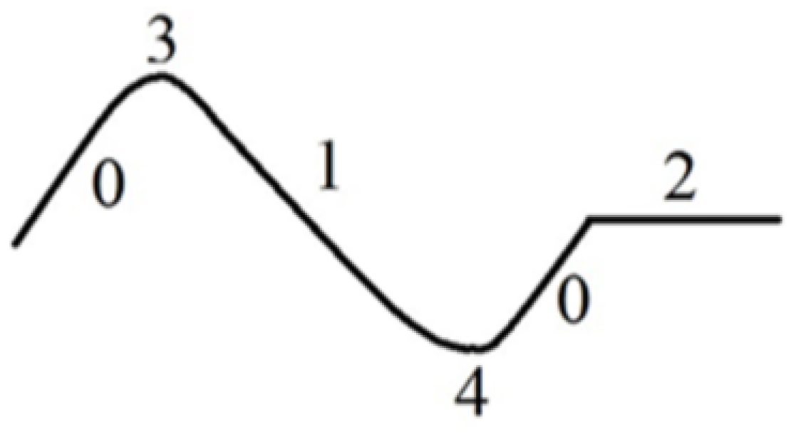
On the basis of the curve morphology principle, a spectral curve can be decomposed to two different morphemes, i.e., fundamental and extended morphemes [24,25,28,29]. The fundamental morpheme describes the segments of the spectral curve, including ascending, descending and flat segments. The extended morpheme is defined as the extreme value at the peak and/or valley of the spectral curve. These morphemes can be symbolized using codes: ascending segment represented as “0”, descending segment “1”, flat segment “2”, and peak and valley of the spectral curve “3” and “4”, respectively. Figure 3 shows an example of the symbolization of a spectral curve.
Based on the above symbolization, the basic variation characteristics (ascending/descending) of a spectral curve can be described. Additionally, a morpheme vector is needed to correctly quantify the spectral curve. Thus, we defined the morpheme vector as B = (T, C0, C1, ..., Cn-1), where T is the morpheme code, and C0,C1, …, Cn-1 denote the n attributes of the morpheme, these are, the numerical values that describe the curve. As mentioned previously, there are two types of morphemes. Therefore, the morpheme vectors were also grouped into a fundamental morpheme vector and an extended morpheme vector that were labeled as Bb and Bs, respectively. Through use of the morpheme vectors, a spectral curve was easily transformed into a 2-D table composed of a series of characteristics. In the 2-D table, the second and subsequent rows refer to the types of various morpheme vectors, and the columns denote the attribute characteristics of each vector. Each vector is composed as follows:
Bb (the basic morpheme vector) = (the morpheme code, the beginning position of morpheme, the ending position of morpheme, and the mean value of morpheme); Bs (the expanded morpheme vector) = (the morpheme code, the sequence number of peak/valley, the position of morpheme, and the value of morpheme).
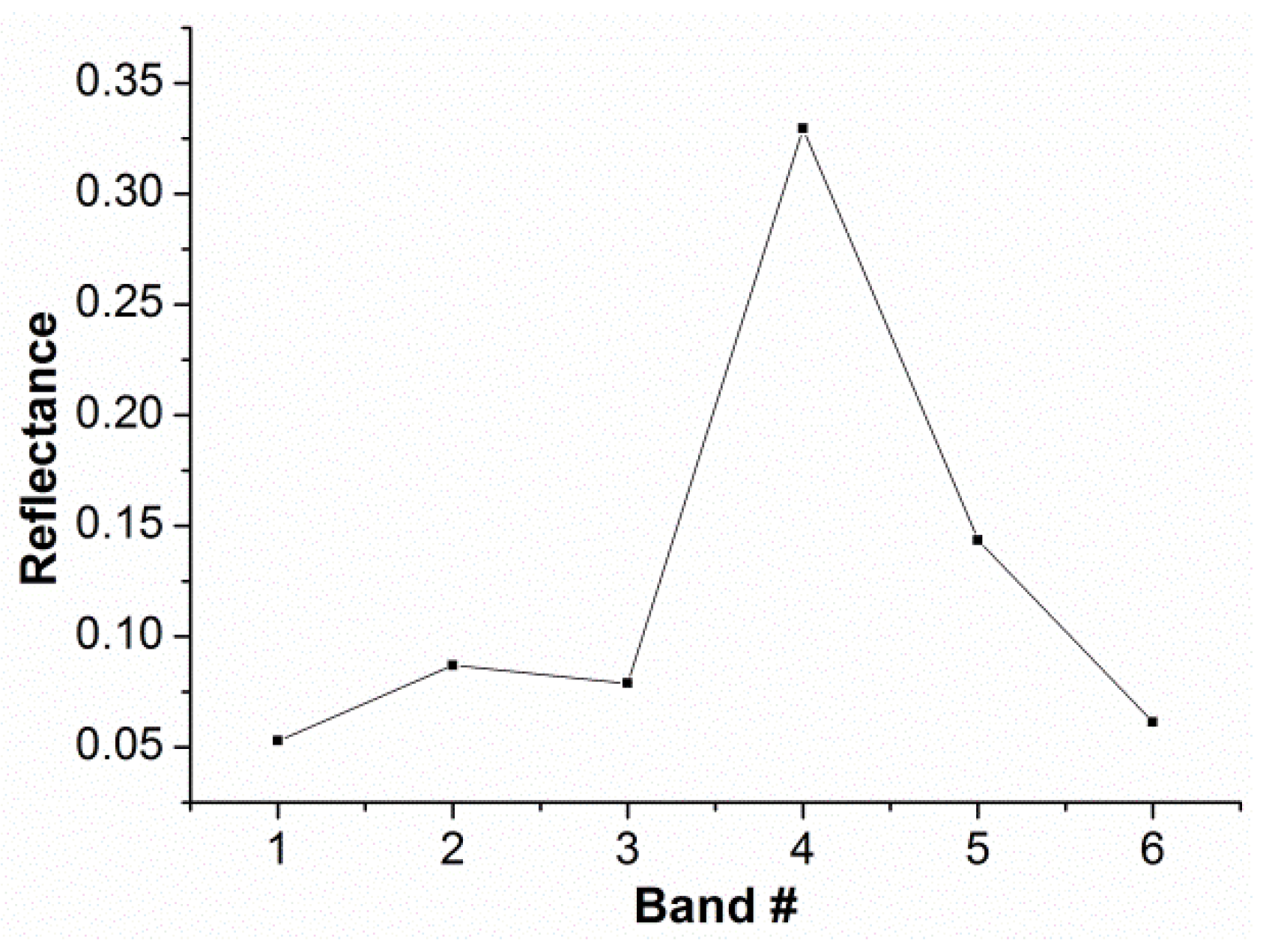
Specific to the remotely sensed data, such as the TM data, the spectral curve shown in Figure 4 is composed of two ascending segments (from bands 1 to 2 and bands 3 to 4, respectively), two descending segments (from bands 2 to 3 and bands 4 to 6, respectively), two peaks (located at bands 2 and 4, respectively) and one valley (located at band 3). Whether bands j to k is the ascending, descending or flat segments is determined by the following criteria outlined in Table 1. Specifically, the ascending, descending or flat segment is between two inflection points, at which the curve changes from decreasing trend to increasing trend, or to flat, and vice versa. Through use of the symbolization method and the attribute composition of each morpheme vector as defined above, the values in Table 2, which show the numerical description of the reflectance spectrum shown in Figure 4, can be obtained.

3.3. Matching of Spectral Shape

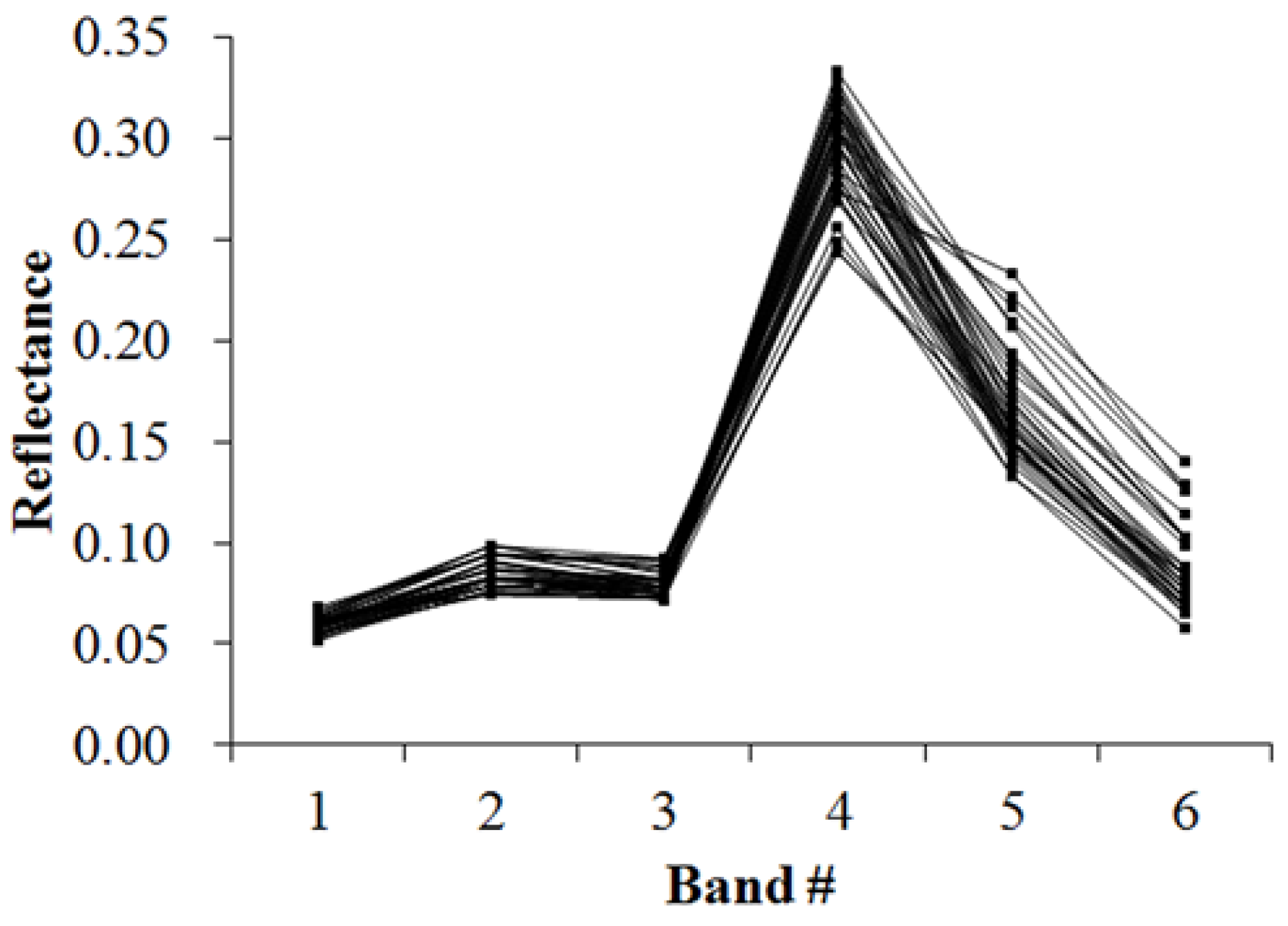
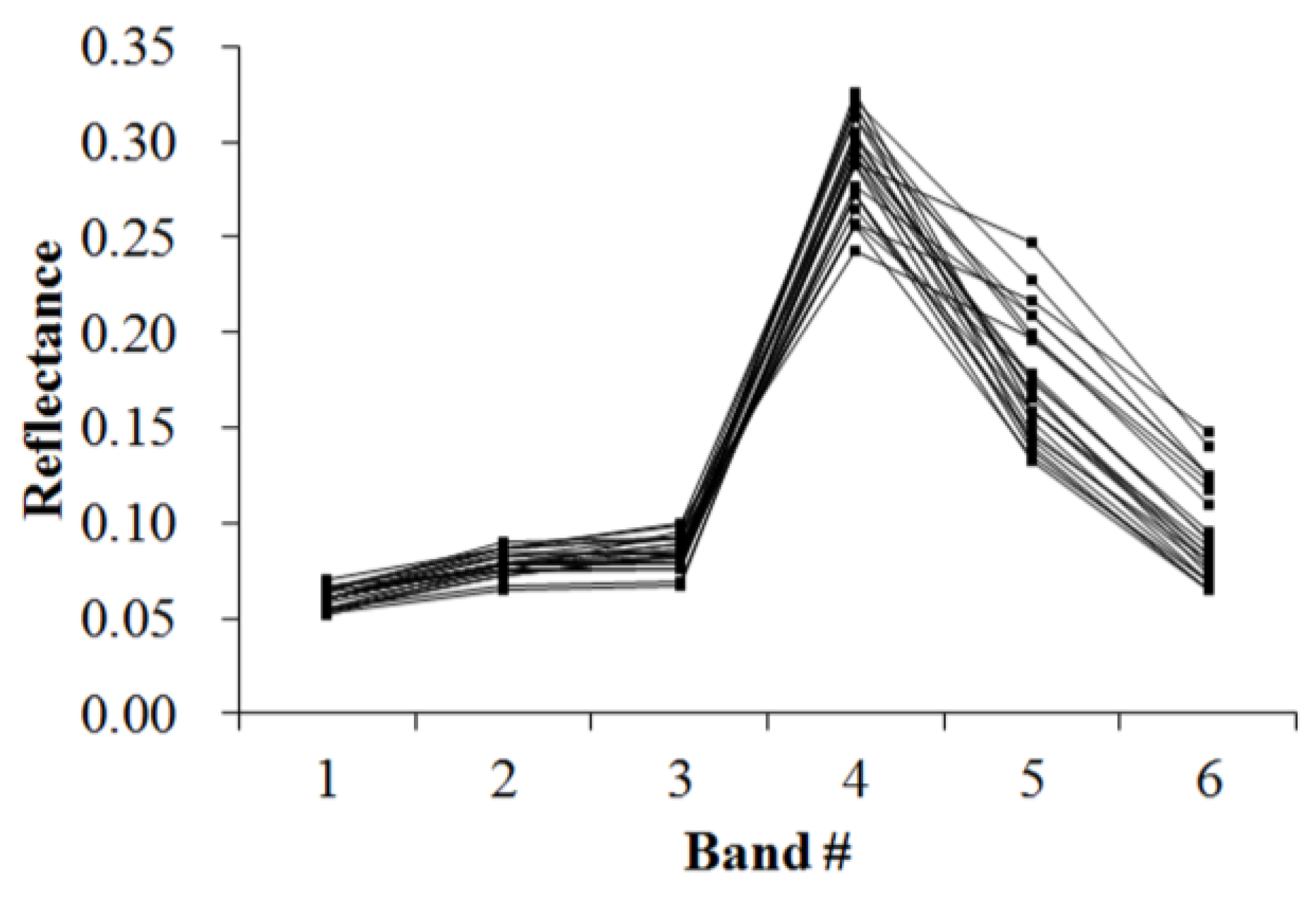
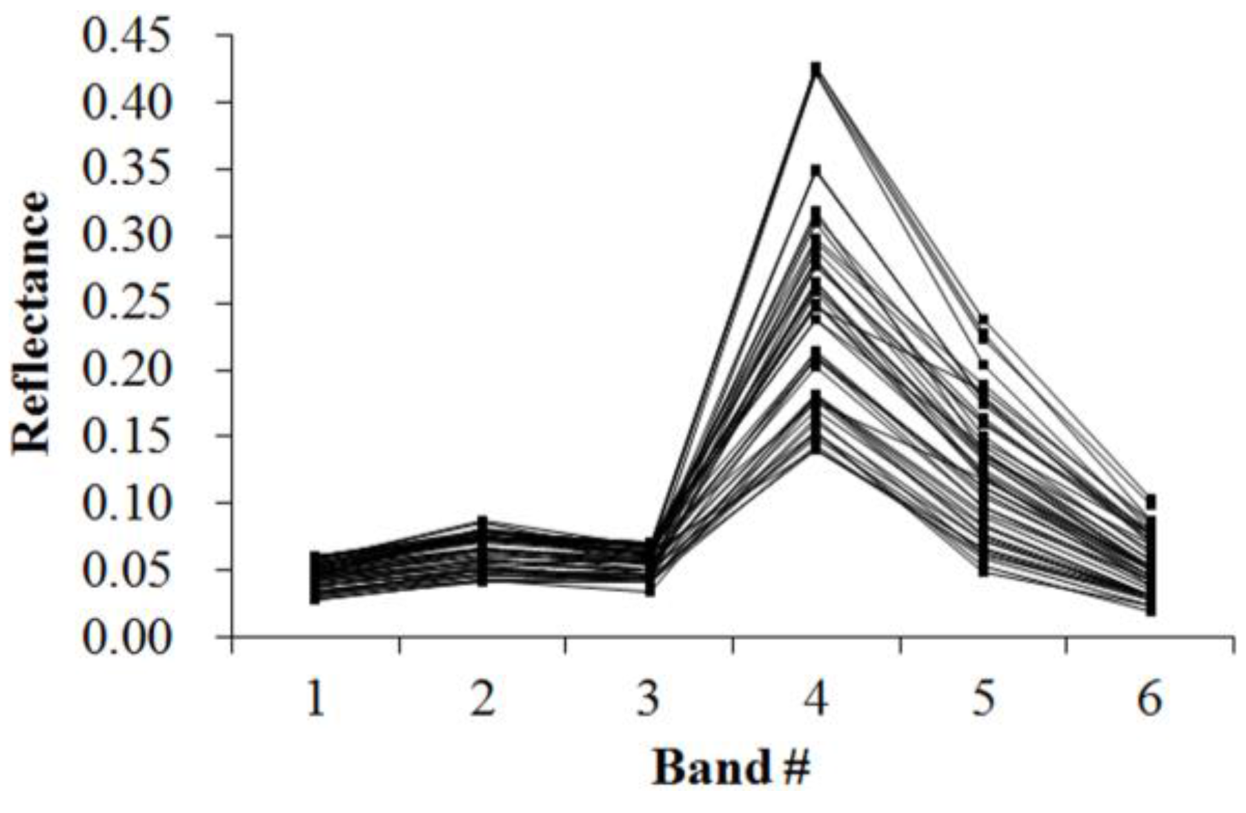
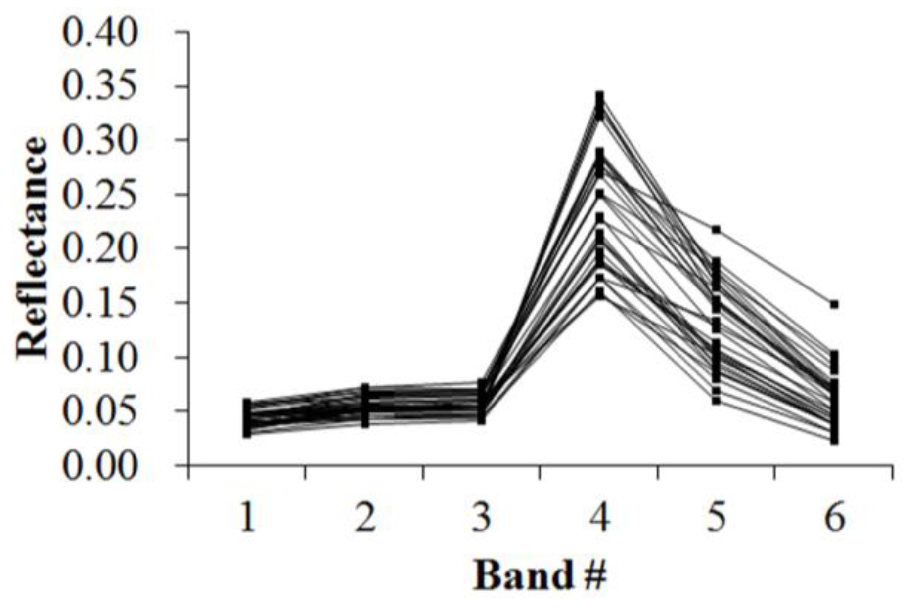
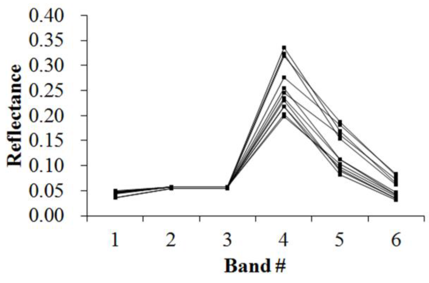
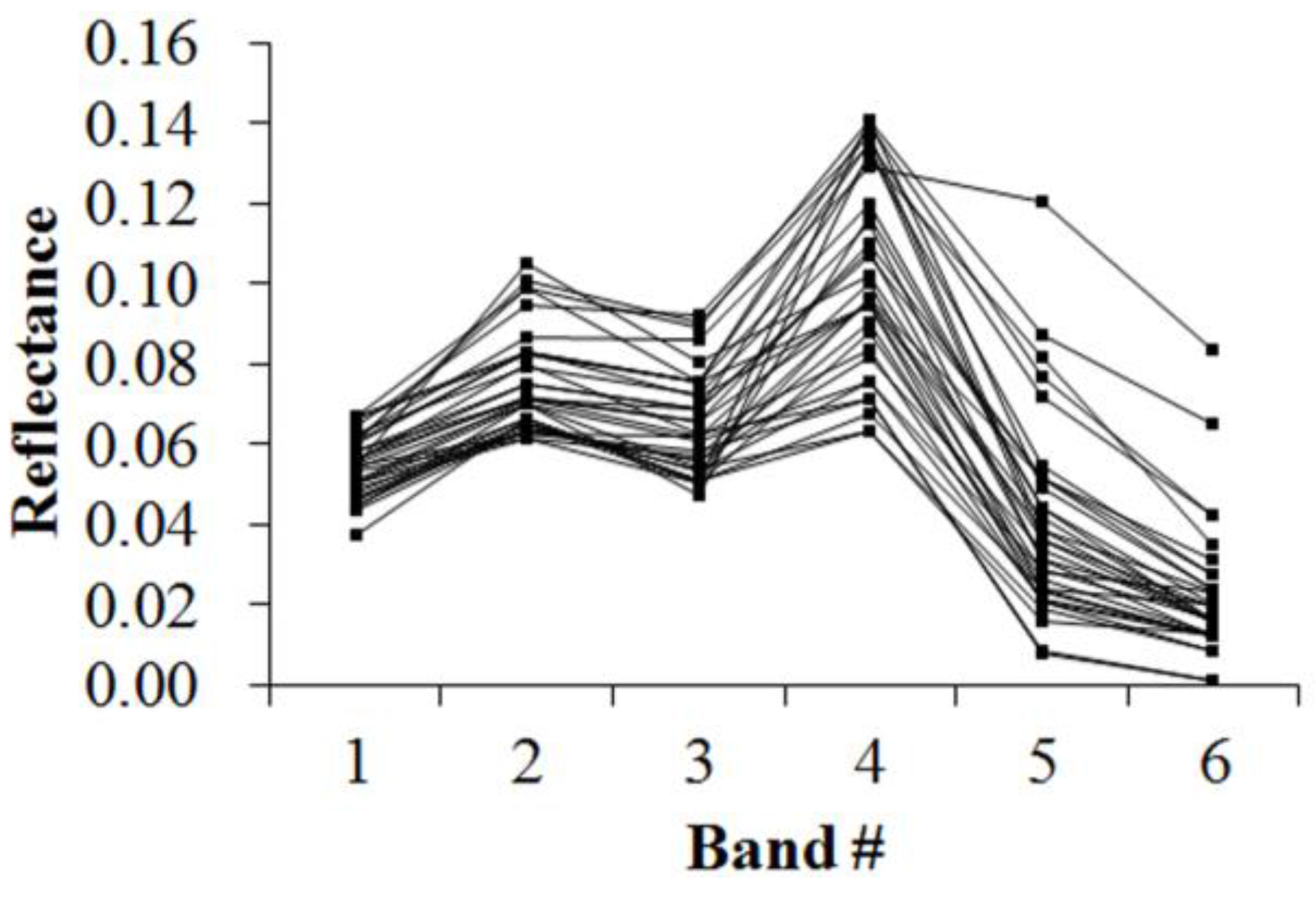
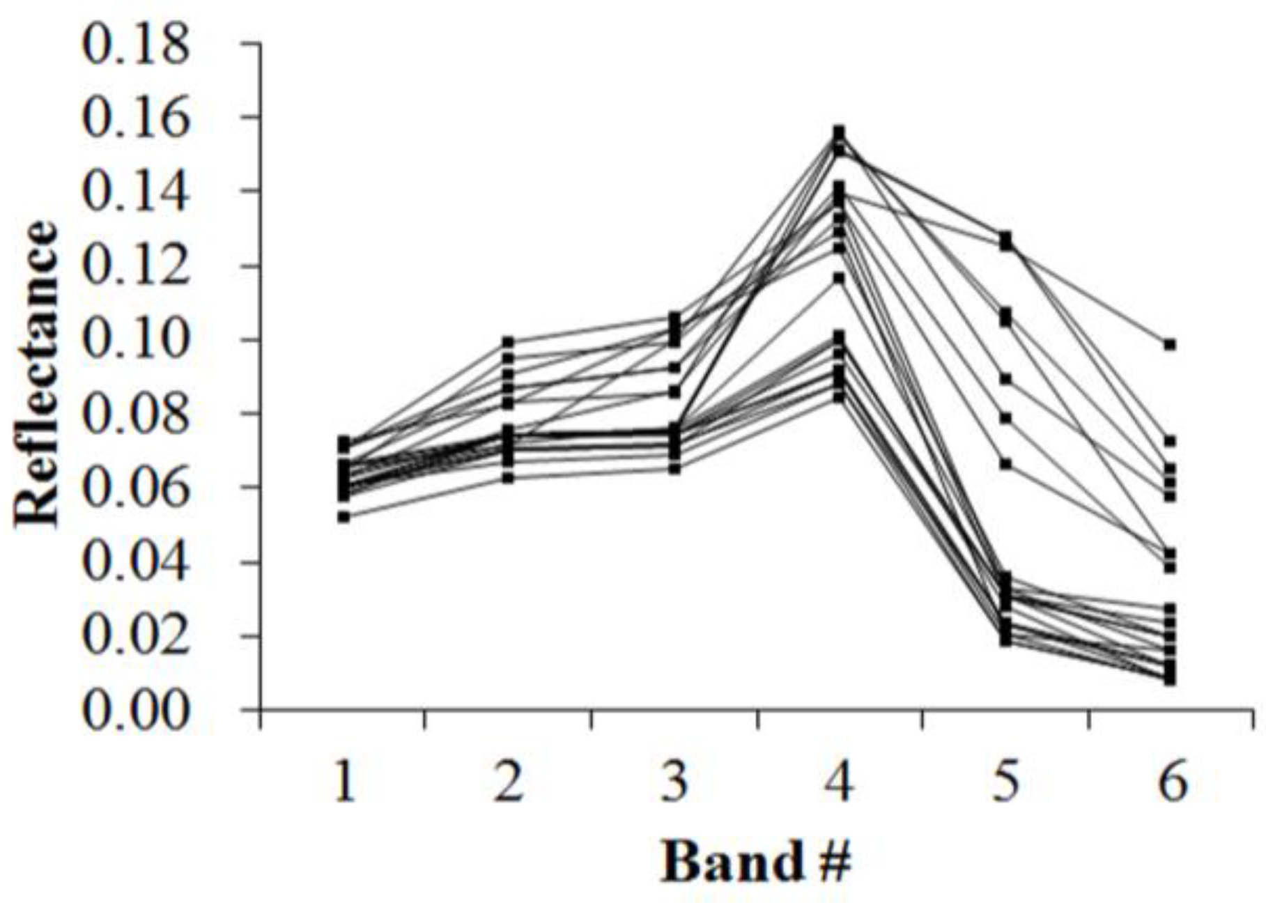
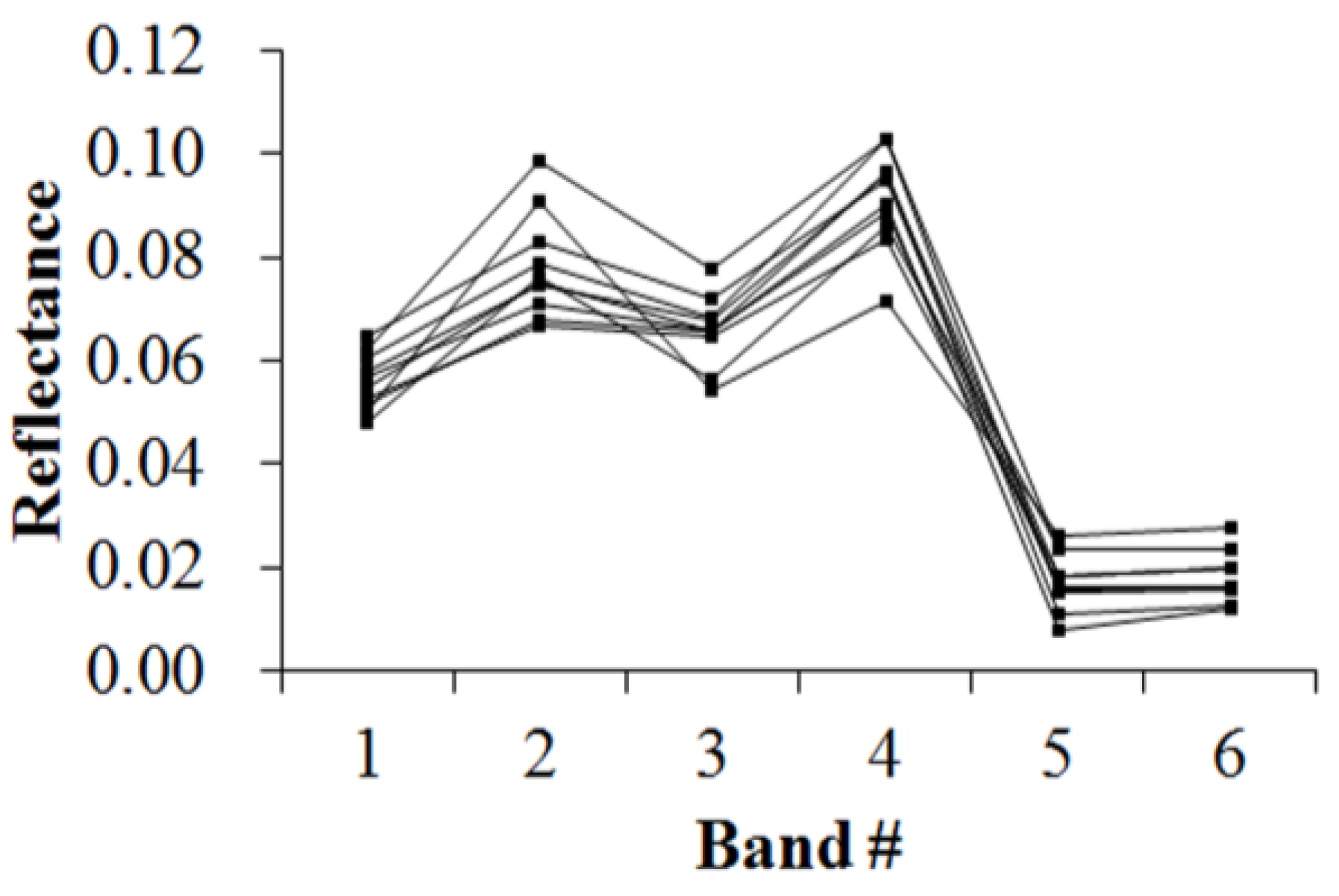
Use of the spectral matching method is necessary to efficiently classify pixels into the known categories. This matching algorithm defines the manner in which unknown or target spectra are compared with the known reference [15]. Here, the characteristics of known reference are called identification templates. Morpheme vector definition for the identification template is similar to those for Table 2, but the last column of the identification template shows the upper and lower limits of a range of measurable characteristic. The design of an identification template requires selection of classification samples that are representative of the spectral characteristics of the classes. It should be noted that remotely sensed image data are known for their high degree of complexity and irregularity [6]. It is necessary to adjust the ranges in the identification template according to the initial identification results to ensure the representativeness of the identification template. Otherwise, the sample data cannot be representative of the spectral variation of that kind of land cover type. Finally, the optimal threshold, which is based on the training samples statistics, must maintain a low number of false alarms and a high number of correct classifications. Figure 5, Figure 6, Figure 7, Figure 8, Figure 9, Figure 10, Figure 11 and Figure 12 display the spectral curves collected from the samples to determine these identification templates (Table 3, Table 4, Table 5, Table 6, Table 7, Table 8, Table 9 and Table 10). By symbolizing the curves in Figure 5, Figure 6, Figure 7, Figure 8, Figure 9, Figure 10, Figure 11 and Figure 12 using the symbolization method descripted in Section 3.2, the corresponding table can be obtained. For the study area B, the identification templates are similar with those of area A, but the suitable thresholds in the last column for area B. The total sample numbers used to determine these identification temples are 224 for area A and 209 for area B. Image objects within the defined limits of identification template are assigned to a specific class, while those outside of the limits are assigned to other classes.
Because of the natural complexity and the fact that the same object has different spectra, more than one identification templates were designed for one kind of object. Meanwhile, one may note that identification templates in Table 3, Table 5 and Table 8 for cropland, forest and water classes, respectively, are similar. The same phenomenon occurs in Table 4, Table 6 and Table 9. This also indicates that different objects have the same spectrum. However, the differences between them lie in the different threshold ranges in the last column in a certain row. Specifically, Table 3 holds the lowest threshold of 0.0718 in the fifth row vs. Table 5 with highest value of 0.0717, and Table 3 holds the lowest threshold of 0.1553 in the seventh row vs. Table 8 with highest value of 0.1408. The different thresholds in similar identification templates, which made the different objects to be separable, were in bold. Table 7 and Table 10, which indicate the unique spectral curve shapes for forest and water classes, respectively, are different from others.
To perform the classification process, a matching algorithm that allows for multilevel matching was used in this study. For a target curve S and the known identification template M, this algorithm is executed according to the following steps: (1) Extract the morpheme vectors (the second to fourth columns) from the 2-D Table describing the target curve S and identification template M, respectively. Each column is represented by a string. Thus, six strings were generated in this step, three for the target curve S and three for the identification template M. (2) Compare the strings for the target curve S with the ones for the identification template M. The same strings indicates the similar shape variation between the target curve S and identification template M. (3) Judge whether the values in the last column of 2-D Table corresponding to the target curve S is within the threshold ranges in the last column of the identification template M. If so, the final match with template M is finished. Matching pixel corresponding to target curve S belongs to the corresponding category of identification template M. The above steps are executed for each pixel. The advantages of this matching algorithm lie in its flexibility and the initial identification by shape variation. If the spectral shape variety of the target curve disaccords with the one of identification template, then the target curve is not assigned to that specific class, despite the similar spectral values.

3.4. Accuracy Assessment

The error matrix method, which is the most common approach for accuracy assessment of categorical classes [30,31], was used in this study to evaluate the accuracy of classified images, with high resolution images from Google Earth as references. To generate the error matrix, a number of samples that are distributed randomly within areas A and B were required. The polynomial distribution-based method was used to calculate the sample number [16]:
N = s i ( 1 s i ) Γ b i 2
where si is the area proportion of class i that is closest to 50% among all classes, bi is the desired accuracy of class i, Γ is the χ2-distribution value with the degree of freedom of 1 and the probability of 1 − (1 − α)/n, α is the confidence level, and n is the number of classes.
Due to the lack of the information on the area proportion of each class, the polynomial distribution algorithm was under the worst case. Following the work of Hu et al. [16], we assumed that the area proportion of each class was 50% of the study area. Equation (1) was then rewritten as:
N = Γ 4 b i 2
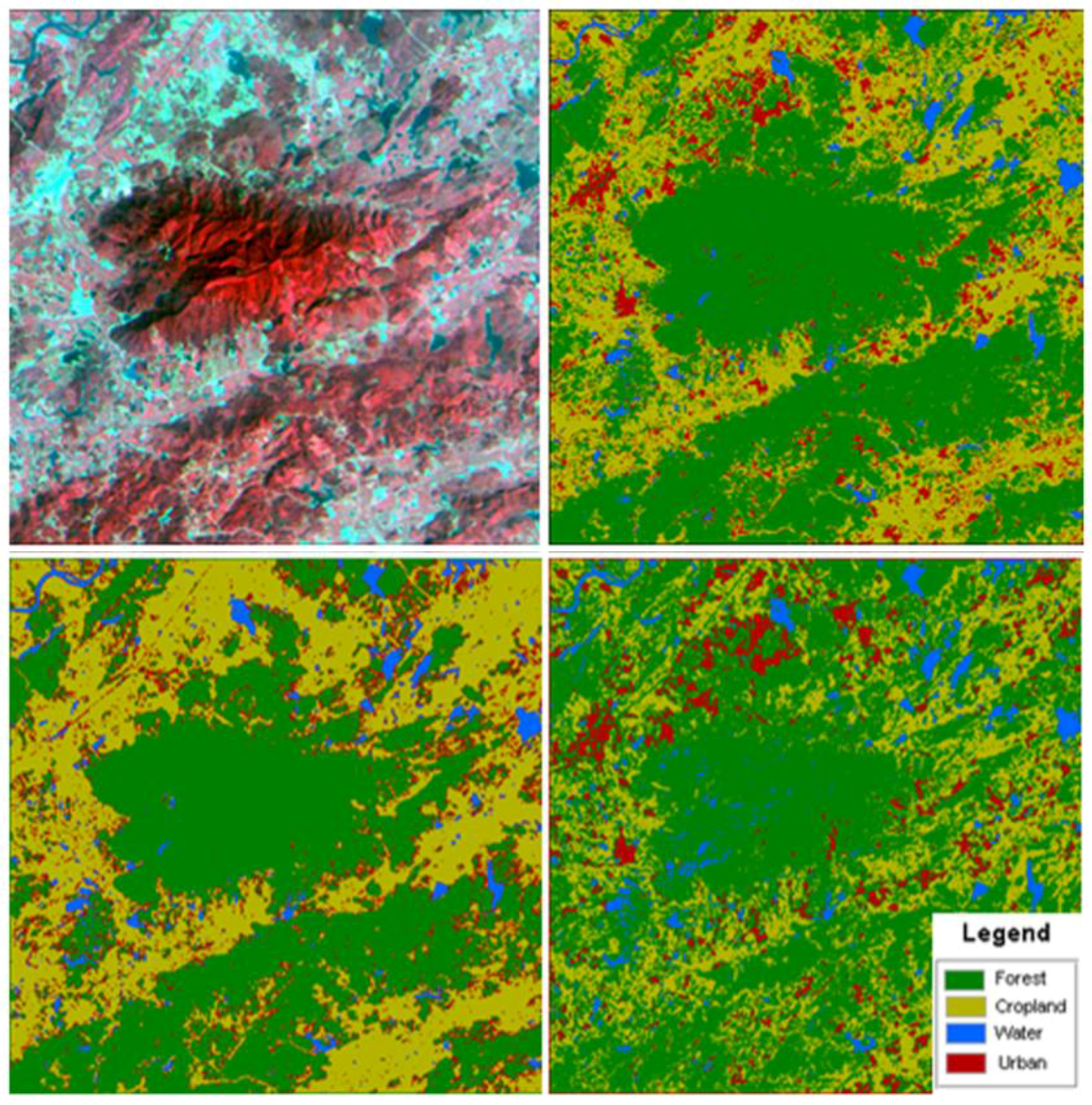
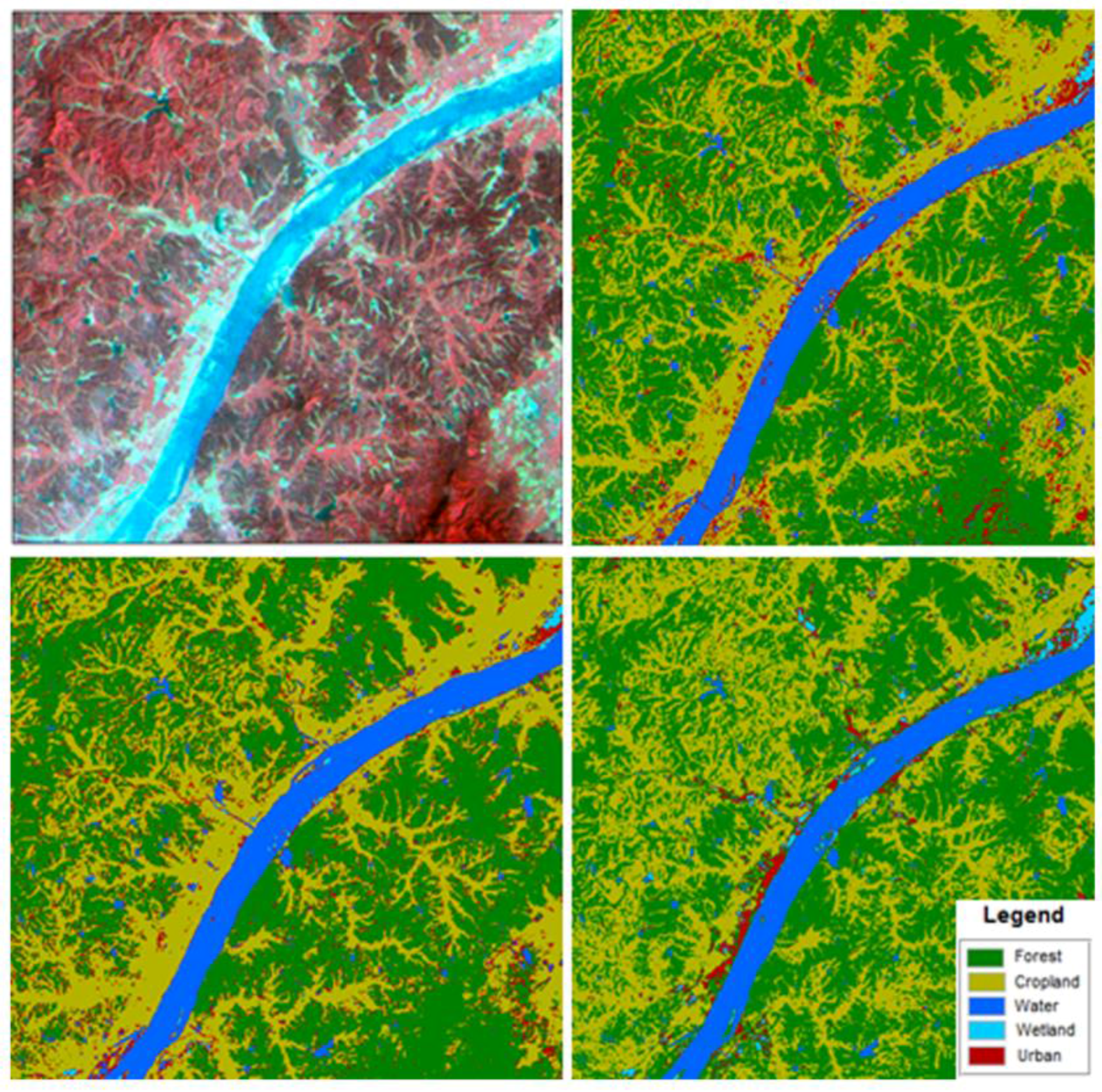
In this study, α was set to 85%, and bi was set to 5%. According to Figure 13 and Figure 14, n was 4 and 5 for areas A and B, respectively. Thus, N is 433 and 471 for areas A and B, respectively. The following statistics will be adopted to evaluate the accuracy of image classification [32]: user’s accuracy (UA), producer’s accuracy (PA), overall accuracy (OA) and Kappa coefficient.

4. Classification Results and Evaluation

4.1. Classification Results

Applying the developed program on the MATLAB platform, the spectral shape-based classification method was performed to classify the subset images. The classified images for areas A and B are shown in Figure 13 and Figure 14, respectively. To facilitate interpretation of the results, the corresponding false-color images are also displayed in Figure 13 and Figure 14. A visual comparison of the land cover maps obtained using the presented method with the false-color images shows a good consistency between them.
In accordance with the random sample points, the error matrixes (Table 11 and Table 12) were produced with the overall accuracy and Kappa coefficients of 0.834 and 0.677 (see Table 13) for Table 11 and 0.854 and 0.748 (see Table 13) for Table 12, respectively. With regard to the individual class, the UA and PA related to forest and cropland classes are more than 0.74 for both areas A and B. Water class shows high UA of 0.94 and PA of 0.97 for area B and the PA (0.63) is generally high for area A. The PA for urban class is above 0.60 for both areas A and B and the UA is low. The wetland class obtains the UA of 0.75 and PA of 0.60. The results indicate a good agreement between the classified maps obtained by spectral shape-based approach and Google Earth high resolution imagery. Therefore, the spectral shape-based classification method is workable and valuable for further research.
Due to two different areas were considered in this study, in order to discover if any accuracy measure was not affected by the area selection, one-way ANOVA tests were performed by using the area as factor and the accuracy values obtained from the two considered areas as response variables [33]. The results showed that UA and PA were not influenced by the area selection at the 95% confident level. Therefore, UA and PA are suitable for the accuracy of classified images.

4.2. Comparison with Other Methods

To ascertain the relative performance of spectral shape-based classification, support vector machine (SVM) and minimum distance (MD) classification methods were also implemented to classify areas A and B. SVM is selected because it has been widely reported as an outstanding classifier in remote sensing [9,34]. In this paper, SVM algorithm was implemented with the radial basis kernel function. The MD algorithm is one of the traditional supervised classification methods and now well-understood. To enable direct comparison between different methods, the same training samples were used for the three methods. Figure 13 and Figure 14 present the classification results, respectively, for areas A and B. Table 13 summarizes the classification accuracy among the three methods. Judging by the total results, the spectral shape-based method obtains the best OA (0.834 for area A and 0.854 for area B) and the Kappa coefficient (0.677 for area A and 0.748 for area B), followed by SVM method. The OA and Kappa coefficient obtained by MD are lowest. With respect to UA, the spectral shape-based classification shows highest value for cropland, water and urban classes in area A and forest, cropland and urban classes in area B. In terms of PA, the statistics obtained by spectral shape-based classification are highest for forest class in area A and for all classes except wetland in area B. The same PA value of 0.6 related to wetland class in area B was obtained by the three methods. One may note that the accuracy of urban class is generally low for these three methods. Since in urban area, the spectral curve of an individual pixel usually cannot represent a single land cover class, but rather a mixture of two or more classes. The definition of spectral shape for an urban class is not reasonable due to incorporating information from other non-urban classes. Therefore, the pixels that were not detected successfully by the non-urban classes considered in the study were assigned to the urban class for all these three methods. The complexity and diversity of urban objects remains a challenge in the detection of urban objects from high resolution satellite data [34,35]. Despite this, the UA obtained by spectral shape-based classification are higher than those by SVM and MD methods for both areas A and B. The PA of urban class obtained by spectral shape-based classification is the same with the one obtained by MD for area A, while better than that by SVM for both areas A and B.
In terms of classification efficiency, spectral shape-based classification takes about 9 min (computer configuration: CPU 2.93 GHz and installed memory 4.00 GB) for each area to execute one time. Both SVM and MD methods take less than 1 min for both areas.

5. Discussion

As a difference from the published classification approaches, this research highlights the shape analysis for classifying remotely sensed data. The shape analysis can catch the subtle difference among different land cover classes, which is often hard to detect with algorithms based on the spectral value characteristics of the whole spectrum, by decomposition of the spectral curve into a number of consecutive segments. Meanwhile, the 2-D Tables presented in this study show not only the spectral variation tendency (ascending/descending), but also the characteristics of each segment (such as the beginning and ending positions, the mean value). By doing this, both spectral shape and spectral value can be used to classify remotely sensed data. Using the spectral shape-based method, the OA of 0.834 for area A and 0.854 for area B and the Kappa coefficient of 0.677 for area A and 0.748 for area B were obtained.
Meanwhile, there are also some drawbacks for the spectral shape-based classification research. The classification accuracy can be affected by the threshold ranges in the identification templates. Suitable variable ranges determined by training samples are critical parameters for successfully implementing the spectral shape-based classification. In addition, compared with other classification methods, the spectral shape-based method is time-consuming. The reasons are attributed to the following two aspects. One is the increasing data dimensions due to describing the curve shape using a 2-D table. The other is the multilevel matching algorithm. The further optimization of matching algorithm and a compiled language alternative to develop this method should reduce the execution time.

6. Conclusions

The spectral curve shape of one surface cover type is usually different from other covers. Spectral shape information derived from remotely sensed data could be applied to discrimination of surface objects. However, it is not easy to quantify the spectral shape, which has resulted in the lack of spectral shape data from most of the current published remotely sensed classification literature. In this paper, a remotely sensed classification method that fully utilizes the spectral shape was developed by parameterizing the spectral shape. The core idea of parameterization is in the coding of the spectral curve shape. In general, the spectral curve is composed of extreme values and some branches (such as ascending branch, descending branch and flat branch). Therefore, it is possible to code and parameterize the object’s spectral curve shape by only using a few numbers. We obtained successfully classification results with OAs 0.834 and 0.854 for two test areas when a matching algorithm was introduced in the course of spectral shape classification. The comparison with SVM and MD methods indicated that the best OAs and Kappa coefficients were obtained by spectral shape-based classification. It should also be noted that the primary motivation for this research was to present a theory of image classification using spectral shape, and only preliminary results were provided in this article. Future study may focus on the following subjects:
(1) The concept of spectral shape can be well demonstrated in hyperspectral images. Therefore, the presented method will be more practically meaningful for hyperspectral data.
(2) The design of identification templates is, to some extent, subjective and restricts further development of this methodology. A necessity for further study is the development of an active machine learning method for determining the appropriate threshold in identification templates.

Acknowledgments

The author Yuanyuan Chen would like to thank the China Scholarship Council for the financially support of her stay in ICube (UMR7357), France. Thanks are also given to the anonymous reviewers for their valuable comments and suggestions.

Author Contributions

Yuanyuan Chen wrote the manuscript and was in charge of the research design and results analysis. Miaozhong Xu processed and analyzed the remotely sensed data; Quanfang Wang and Zhao-Liang Li conceived the research. Yanlong Wang and Si-Bo Duan collected the remotely sensed data and designed the research.

Conflicts of Interest

The authors declare no conflict of interest.

References

  1. Colditz, R.R.; López Saldaña, G.; Maeda, P.; Espinoza, J.A.; Tovar, C.M.; Hernández, A.V.; Benítez, C.Z.; Cruz López, I.; Ressl, R. Generation and analysis of the 2005 land cover map for Mexico using 250 m MODIS data. Remote Sens. Environ. 2012, 123, 541–552. [Google Scholar] [CrossRef]
  2. Friedl, M.A.; McIver, D.K.; Hodges, J.C.F.; Zhang, X.Y.; Muchoney, D.; Strahler, A.H.; Woodcocka, C.E.; Gopal, S.; Schneider, A.; Cooper, A.; et al. Global land cover mapping from MODIS algorithms and early results. Remote Sens. Environ. 2002, 83, 287–302. [Google Scholar] [CrossRef]
  3. Amarsaikhan, D.; Douglas, T. Data fusion and multisource image classification. Int. J. Remote Sens. 2004, 25, 3529–3539. [Google Scholar] [CrossRef]
  4. Barandela, R.; Juarez, M. Supervised classification of remotely sensed data with ongoing learning capability. Int. J. Remote Sens. 2002, 23, 4965–4970. [Google Scholar] [CrossRef]
  5. Belgiu, M.; Drǎguţ, L. Comparing supervised and unsupervised multiresolution segmentation approaches for extracting buildings from very high resolution imagery. ISPRS J. Photogramm. Remote Sens. 2014, 96, 67–75. [Google Scholar] [CrossRef] [PubMed]
  6. Kavzoglu, T. Increasing the accuracy of neural network classification using refined training data. Environ. Modell. Softw. 2009, 24, 850–858. [Google Scholar] [CrossRef]
  7. Xu, L.; Li, J.; Brenning, A. A comparative study of different classification techniques for marine oil spill identification using RADARSAT-1 imagery. Remote Sens. Environ. 2014, 141, 14–23. [Google Scholar] [CrossRef]
  8. Carrão, H.; Gonçalves, P.; Caetano, M. Contribution of multispectral and multitemporal information from MODIS images to land cover classification. Remote Sens. Environ. 2008, 112, 986–997. [Google Scholar] [CrossRef]
  9. Foody, G.M.; Mathur, A. The use of small training sets containing mixed pixels for accurate hard image classification: Training on mixed spectral responses for classification by a SVM. Remote Sens. Environ. 2006, 103, 179–189. [Google Scholar] [CrossRef]
  10. Hansen, M.C.; DeFries, R.S.; Townshend, J.R.; Sohlberg, R. Global land cover classification at 1 km spatial resolution using a classification tree approach. Int. J. Remote Sens. 2000, 21, 1331–1364. [Google Scholar] [CrossRef]
  11. Xu, M.; Watanachaturaporn, P.; Varshney, P.; Arora, M. Decision tree regression for soft classification of remote sensing data. Remote Sens. Environ. 2005, 97, 322–336. [Google Scholar] [CrossRef]
  12. Blaschke, T. Object based image analysis for remote sensing. ISPRS J. Photogramm. Remote Sens. 2010, 65, 2–16. [Google Scholar] [CrossRef]
  13. Namdar, M.; Adamowski, J.; Saadat, H.; Sharifi, F.; Khiri, A. Land-use and land-cover classification in semi-arid regions using independent component analysis (ICA) and expert classification. Int. J. Remote Sens. 2014, 35, 8057–8073. [Google Scholar] [CrossRef]
  14. Li, Q.; Wang, C.; Zhang, B.; Lu, L. Object-based crop classification with Landsat-MODIS enhanced time-series data. Remote Sens. 2015, 7, 16091–16107. [Google Scholar] [CrossRef]
  15. Padma, S.; Sanjeevi, S. Jeffries Matusita based mixed-measure for improved spectral matching in hyperspectral image analysis. Int. J. Appl. Earth Obs. Geoinf. 2014, 32, 138–151. [Google Scholar] [CrossRef]
  16. Hu, Q.; Wu, W.; Xia, T.; Yu, Q.; Yang, P.; Li, Z.; Song, Q. Exploring the use of Google Earth imagery and object-based methods in land use/cover mapping. Remote Sens. 2013, 5, 6026–6042. [Google Scholar] [CrossRef]
  17. Peña-Barragán, J.M.; Ngugi, M.K.; Plant, R.E.; Six, J. Object-based crop identification using multiple vegetation indices, textural features and crop phenology. Remote Sens. Environ. 2011, 115, 1301–1316. [Google Scholar] [CrossRef]
  18. Sun, C.; Wu, Z.-F.; Lv, Z.-Q.; Yao, N.; Wei, J.-B. Quantifying different types of urban growth and the change dynamic in Guangzhou using multi-temporal remote sensing data. Int. J. Appl. Earth Obs. Geoinf. 2013, 21, 409–417. [Google Scholar] [CrossRef]
  19. Verbesselt, J.; Zeileis, A.; Herold, M. Near real-time disturbance detection using satellite image time series. Remote Sens. Environ. 2012, 123, 98–108. [Google Scholar] [CrossRef]
  20. Wardlow, B.; Egbert, S.; Kastens, J. Analysis of time-series MODIS 250 m vegetation index data for crop classification in the U.S. Central Great Plains. Remote Sens. Environ. 2007, 108, 290–310. [Google Scholar] [CrossRef]
  21. Dennison, P.E.; Roberts, D.A.; Peterson, S.H. Spectral shape-based temporal compositing algorithms for MODIS surface reflectance data. Remote Sens. Environ. 2007, 109, 510–522. [Google Scholar] [CrossRef]
  22. Shanmugam, S.; SrinivasaPerumal, P. Spectral matching approaches in hyperspectral image processing. Int. J. Remote Sens. 2014, 35, 8217–8251. [Google Scholar] [CrossRef]
  23. Li, J.; Narayanan, R.M. A shape-based approach to change detection of lakes using time series remote sensing images. IEEE Trans. Geosci. Remote 2003, 41, 2466–2477. [Google Scholar]
  24. Dupé, F.-X.; Luc, B. Tree covering within a graph kernel framework for shape classification. ICIAP 2009, 278–287. [Google Scholar]
  25. Lin, P.; Xu, J. A description and recognition method of curve configuration and its application. J. South China Univ. Technol. (Nat. Sci. Ed.) 2009, 37, 77–81. [Google Scholar]
  26. Kayani, W. Shape Based Classification and Functional Forecast of Traffic Flow Profiles. Ph.D. Thesis, Missouri University of Science and Technology, Rolla, MO, USA, 2015. [Google Scholar]
  27. Oyama, Y.; Matsushita, B.; Fukushima, T. Distinguishing surface cyanobacterial blooms and aquatic macrophytes using Landsat/TM and ETM+ shortwave infrared bands. Remote Sens. Environ. 2015, 157, 35–47. [Google Scholar] [CrossRef]
  28. Lines, J.; Davis, L.M.; Hills, J.; Bagnall, A. A shapelet transform for time series classification. In Proceedings of the 18th ACM SIGKDD International Conference on Knowledge Discovery and Data Mining, Beijing, China, 12–16 August 2012.
  29. Mehtre, B.M.; Kankanhalli, M.S.; Lee, W.F. Shape measurement for content based image retrieval: A comparison. Inf. Process. Manag. 1997, 33, 319–337. [Google Scholar] [CrossRef]
  30. Comber, A.; Fisher, P.; Brunsdon, C.; Khmag, A. Spatial analysis of remote sensing image classification accuracy. Remote Sens. Environ. 2012, 127, 237–246. [Google Scholar] [CrossRef]
  31. Lu, D.; Weng, Q. A survey of image classification methods and techniques for improving classification performance. Int. J. Remote Sens. 2007, 28, 823–870. [Google Scholar] [CrossRef]
  32. Denham, R.; Mengersen, K.; Witte, C. Bayesian analysis of thematic map accuracy data. Remote Sens. Environ. 2009, 113, 371–379. [Google Scholar] [CrossRef]
  33. Arcidiacono, C.; Porto, S.M.C.; Cascone, G. Accuracy of crop-shelter thematic maps: A case study of maps obtained by spectral and textural classification of high-resolution satellite images. J. Food Agric. Environ. 2012, 10, 1071–1074. [Google Scholar]
  34. Momeni, R.; Aplin, P.; Boyd, D. Mapping complex urban land cover from spaceborne imagery: The influence of spatial resolution, spectral band set and classification approach. Remote Sens. 2016, 8, 88. [Google Scholar] [CrossRef]
  35. Erener, A. Classification method, spectral diversity, band combination and accuracy assessment evaluation for urban feature detection. Int. J. Appl. Earth Obs. Geoinf. 2013, 21, 397–408. [Google Scholar] [CrossRef]
Figure 1. Geolocation of the study area. Two subset images (upper): area A and (lower): area B in false-color (R: band 4, G: band 3, and B: band 2) were used to perform the spectral shape-based image classification.
Ijgi 05 00154 g001
Figure 2. Spectral curves of the cropland (red line) and forest (black line) classes, from remotely sensed data.
Ijgi 05 00154 g002
Figure 3. Symbolization of a spectral curve. (Ascending segment: 0, descending segment: 1, flat segment: 2, and peak and valley of the spectral curve: 3 and 4, respectively).
Ijgi 05 00154 g003
Figure 4. A spectral curve from remotely sensed data.
Ijgi 05 00154 g004
Figure 5. Spectral curves collected from samples used to determine Table 3.
Ijgi 05 00154 g005
Figure 6. Spectral curves collected from samples used to determine Table 4.
Ijgi 05 00154 g006
Figure 7. Spectral curves collected from samples used to determine Table 5.
Ijgi 05 00154 g007
Figure 8. Spectral curves collected from samples used to determine Table 6.
Ijgi 05 00154 g008
Figure 9. Spectral curves collected from samples used to determine Table 7.
Ijgi 05 00154 g009
Figure 10. Spectral curves collected from samples used to determine Table 8.
Ijgi 05 00154 g010
Figure 11. Spectral curves collected from samples used to determine Table 9.
Ijgi 05 00154 g011
Figure 12. Spectral curves collected from samples used to determine Table 10.
Ijgi 05 00154 g012
Figure 13. The subset image for area A in false-color ((upper left) R: band 4, G: band 3, B: band 2) and classified image using (upper right) spectral shape-based method, (lower left) SVM method and (lower right) MD method.
Ijgi 05 00154 g013
Figure 14. The subset image for area B in false-color ((upper left) R: band 4, G: band 3, B: band 2) and classified image using (upper right) spectral shape-based method, (lower left) SVM method and (lower right) MD method.
Ijgi 05 00154 g014
Table 1. The criteria for determination of morphemes in a spectral curve.
AscendingDescendingFlat
Criteriapj < pj + 1 < … < pj + kpj > pj + 1 >…> pj + kpj = pj + 1 = … = pj + k
pj − 1 > pjpj − 1 < pjpj − 1 < pj or pj − 1 > pj
pj + k > pj + k + 1pj + k < pj + k + 1pj + k < pj + k + 1 or pj + k > pj + k + 1
p: the reflectance in certain band; j and k: the sequence numbers of the band.
Table 2. The 2-D table corresponding to the curve in Figure 4.
Name of VectorElement of Vector
Bb0120.0699
Bs3120.0869
Bb1230.0829
Bs4130.0788
Bb0340.2042
Bs3240.3295
Bb1460.1781
Table 3. Identification template 1 for cropland class.
Name of VectorElement of Vector
Bb012[0.0641,0.0827]
Bs312[0.0746,0.0990]
Bb123[0.0733,0.0958]
Bs413[0.0718,0.0925]
Bb034[0.1154,0.2065]
Bs324[0.1553,0.3333]
Bb146[0.0832,0.2172]
Table 4. Identification template 2 for cropland class.
Name of VectorElement of Vector
Bb014[0.1209,0.1409]
Bs314[0.2430,0.3258]
Bb146[0.1532,0.2255]
Table 5. Identification template 1 for forest class.
Name of VectorElement of Vector
Bb012[0.0354,0.0722]
Bs312[0.0422,0.0865]
Bb123[0.0384,0.0773]
Bs413[0.0342,0.0717]
Bb034[0.0925,0.2466]
Bs324[0.1409,0.4260]
Bb146[0.0715,0.2554]
Table 6. Identification template 2 for forest class.
Name of VectorElement of Vector
Bb014[0.0702,0.1208]
Bs314[0.1570,0.3415]
Bb146[0.0812,0.2124]
Table 7. Identification template 3 for forest class.
Name of VectorElement of Vector
Bb012[0.0455,0.0541]
Bb223[0.0440,0.0572]
Bb034[0.1032,0.1967]
Bs314[0.1815,0.3363]
Bb146[0.1009,0.1956]
Table 8. Identification template 1 for water class.
Name of VectorElement of Vector
Bb012[0.0519,0.0829]
Bs312[0.0612,0.1050]
Bb123[0.0557,0.0957]
Bs413[0.0474,0.0925]
Bb034[0.0571,0.1150]
Bs324[0.0634,0.1408]
Bb146[0.0268,0.1112]
Table 9. Identification template 2 for water class.
Name of VectorElement of Vector
Bb014[0.0661,0.1033]
Bs314[0.0837,0.1564]
Bb146[0.0370,0.1214]
Table 10. Identification template 3 for water class.
Name of VectorElement of Vector
Bb012[0.0596,0.0804]
Bs312[0.0667,0.0986]
Bb123[0.0658,0.0883]
Bs413[0.0542,0.0779]
Bb034[0.0629,0.0903]
Bs324[0.0716,0.1028]
Bb145[0.0489,0.0630]
Bs425[0.0079,0.0263]
Bb056[0.0100,0.0269]
Table 11. Error matrix between classified and Google Earth images for area A.
Reference image Category ForestCroplandWater BodyUrbanTotal
Forest24427 6277
Cropland16102 14132
Water2310116
Urban12 58
Total2631341026433
Table 12. Error matrix between classified and Google Earth images for area B.
Reference image Category ForestCroplandWater BodyUrbanWetlandTotal
Forest23244 6 282
Cropland4128181142
Water1 33 34
Urban 116 8
Wetland 1 135
Total23717435214471
Table 13. Comparison of accuracy measurements for areas A and B.
Spectral Shape-Based ClassificationSVMMD
Area AArea BArea AArea BArea AArea B
UAPAUAPAUAPAUAPAUAPAUAPA
Forest0.930.880.980.820.960.780.970.730.790.820.820.70
Cropland0.760.770.740.900.750.850.700.890.560.440.540.71
Water1.000.630.940.970.870.810.940.910.850.690.970.85
Urban0.190.630.290.750.020.130.050.250.170.630.130.13
Wetland 0.750.60 1.000.60 0.380.60
OA0.8340.8540.7900.7810.6950.701
Kappa0.6770.7480.6250.6400.3900.477
* PA: producer’s accuracy, UA: user’s accuracy and OA: overall accuracy.