Pull-Based Modeling and Algorithms for Real-Time Provision of High-Frequency Sensor Data from Sensor Observation Services

Abstract

The widely used pull-based method for high-frequency sensor data acquisition from Sensor Observation Services (SOS) is not efficient in real-time applications; therefore, further attention must be paid to real-time mechanisms in the provision process if sensor webs are to achieve their full potential. To address this problem, we created a data provision problem model, and compare the recursive algorithm Kalman Filter (KF) and our two proposed self-adaptive linear algorithms Harvestor Additive Increase and Multiplicative Decrease (H-AIMD) and Harvestor Multiplicative Increase and Additive Decrease (H-MIAD) with the commonly used Static Policy, which requests data with an unchanged time interval. We also developed a comprehensive performance evaluation method that considers the real-time capacity and resource waste to compare the performance of the four data provision algorithms. Experiments with real sensor data show that the Static Policy needs accurate priori parameters, Kalman Filter is most suitable for the data provision of sensors with long-term stable time intervals, and H-AIMD is the steadiest with better efficiency and less delayed number of data while with a higher resource waste than the others for data streams with much fluctuations in time intervals. The proposed model and algorithms are useful as a basic reference for real-time applications by pull-based stream data acquisition.

1. Introduction

The detection and early warning of emerging natural hazards and man-made disasters require real-time geographic information to support effective and timely emergency response. A lot of sensors are deployed all over the world, continuously monitoring features and geo-objects on the Earth’s surface [1,2], such as mining industry [3], agriculture [4,5], metropolis [6], and atmosphere [7], producing geographic data unceasingly. Given the development of service-oriented science [8], data can be accessed by anyone, from anywhere and in any form [9]. However, sensor observations must be acquired in real-time [3,10] for numerous applications through easily accessible data services; however, existing provision methods lack effective and efficient real-time data acquisition mechanisms.

Open GIS Consortium (OGC) proposed the Sensor Web Enablement (SWE) in 2003, which includes a series of service standards for the sensor web. With these uniform definitions, sensor data can be discovered and obtained through standard protocols and interfaces. Thus, applications could be built on the service standards without considering the underlying communication details between sensors and hardware implementations [11]. One of the very important SWE interface models is the Sensor Observation Service (SOS), whose data access mechanism is pull-based [12]. A middle layer architecture [13] had filled the gap between the sensor networks and the Internet; however, it does not consider how sensor data could be acquired by the consumers from the SOS in real-time.

Service registration and discovery of SOS [14,15,16] and data access methods [17] had been studied. However, this work has focused on how data could be adapted and published by SWE services from the sensors. Few researchers have considered the subsequent data flow from SOS to users, especially for the high-frequency continuous data streams to the real-time application databases. The changing sensor observation frequency due to the dynamic nature of real world phenomena makes it more challenging to effectively get real-time sensor data. A major problem occurs when delineating a high-efficiency data provision system since machines have different working space sizes and speeds, so they will likewise have different observation frequencies [18].

Two data access methods for the sensor web were offered for European Environment Agency (EEA) [17]. The first provides a uniform interface, waiting for data being pushed by the data provider. It is a time-efficient means and does not have to deploy servers to publish data. The other access method sends data requests to the SOS in a fixed frequency, namely the Static Policy, by the Harvestor, a data collecting module. It is a pull-based active method that determines what content to get and at what frequency. Hence, the former is suitable for large institutions like the EEA that are responsible for providing uniform interfaces to push data into databases. In contrast, the latter is more flexible and customizable but less time efficient. Moreover, most of the current sensor web services for data access are pull-based [19]. Therefore, there is an urgent need for dynamic solutions to solve the system stochastic problem of the predefined schedule methods [20].

Many factors can give rise to dynamic problems that are one of the main concerns of current real-time sensor applications. The time interval between two observations can hardly remain the same for several reasons. Environment noise is the most common one. For example, huge buildings could influence the transformation of sensor signals, or harsh weather can also affect hardware conditions. Another reason is artificial interventions or dynamic adjustments. Some smart sensors could auto change their observation frequency depending on the state of the objects they are monitoring. Additionally, hardware failure could cause a long-term interruption, which also changes the observation time intervals.

Besides the dynamic characteristics of sensor observations, the ability to handle dynamic and high-frequency sensor data flows is rather weak in current real-time applications. Numerous sensors produce high-frequency and dynamic data in hours, minutes or even seconds. At the same time, due to the large number of sensors, the data volume generated in real-time is rather huge; thus, resources like network bandwidth and data server load should be considered deliberatively. Most sensor data, however, are currently acquired as static history records and imported to various databases with specific tools all at once. Moreover, the commonly used Static Policy for real-time sensor data acquisition from SOS either has a limited time-efficiency or wastes a lot of resources if the time interval is not preset properly. Therefore, a dynamic model and adaptive algorithms, with high time-efficiency and low resource waste, are needed for real-time applications of high-frequency sensor data flows.

Several algorithms could be considered for adjustment for data provision if they can forecast with very little computation. The Kalman Filter (KF) is an efficient algorithm widely used, such as in the measurement of power system frequency [21], data assimilation [22], and data fusion [23]. It can also be used as a prediction algorithm since it includes a prediction equation set, which can act as an a priori estimation of the current state before a current measurement is produced. Therefore, it is reasonable to introduce the KF as a recursive algorithm into real-time sensor data provision applications. As opposed to the KF, considerable research has focused on the activation algorithms of rechargeable sensors [20,24,25,26]. Madakasira [26] analyzed the recharging process of sensors and compared the performance of four linear recharge algorithms: Additive Increase Multiplicative Decrease (AIMD), Additive Increase Additive Decrease (AIAD), Multiplicative Increase Multiplicative Decrease (MIMD), and Multiplicative Increase Additive Decrease (MIAD). They determine the next sleep interval of sensors according to the energy levels. These two algorithms, AIMD and MIAD, based on this analysis, could be adapted and used as linear algorithms for real-time forecasting in sensor data provision.

Based on the analysis of dynamic problems and algorithms, which could perform forecasting tasks, we modeled the pull-based process of real-time sensor data provision from sensor observation services, and four policies are discussed in terms of the proposed model. Our objective was to minimize the data acquisition time latency, delayed number of data, and resource costs in the system. In turn, we developed a normalized comprehensive performance evaluation method considering real-time performance and resource waste to compare these algorithms in our real time data provision model. Most experiments in data acquisition research in the sensor hardware field are based on simulated data. Our experiments, however, are based on three kinds of real sensor data. With our work, better algorithms than the Static Policy in various real-time sensor data provision applications are found, with improved time-efficiency and redundant requests, and more practical applicability in situations with non-strict-fixed time interval observations.

The remainder of the paper is organized as follows. The introduction of data streams of sensor web is in Section 2, followed by our method in Section 3, in which we define the problem model in Section 3.1, describe the provision policies and performance evaluation methods in Section 3.2 and Section 3.3. The experiments and results are presented in Section 4. Then, the model and algorithms are discussed in Section 5. Section 6 concludes the paper.

2. The Data Streams from Sensor Webs

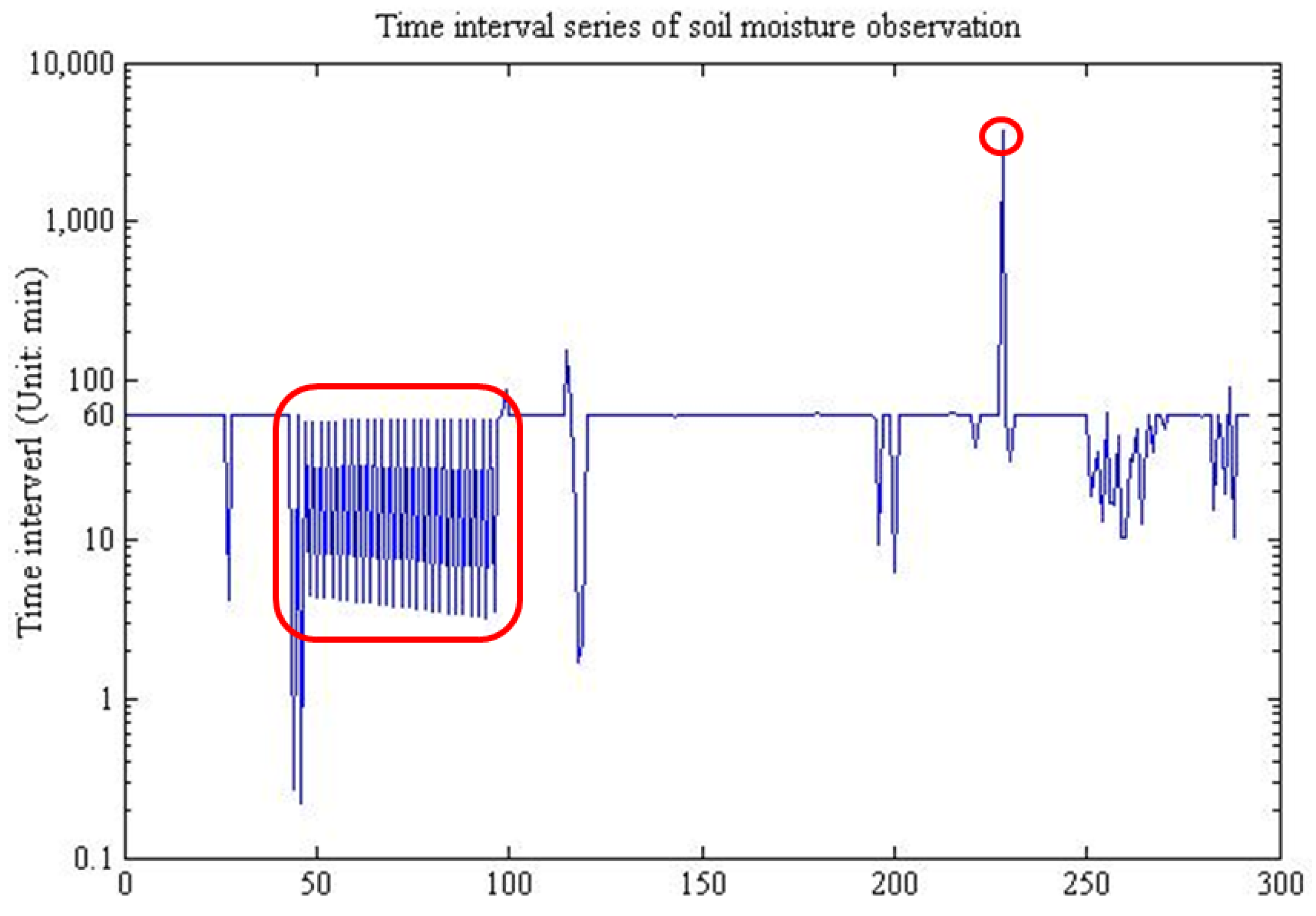
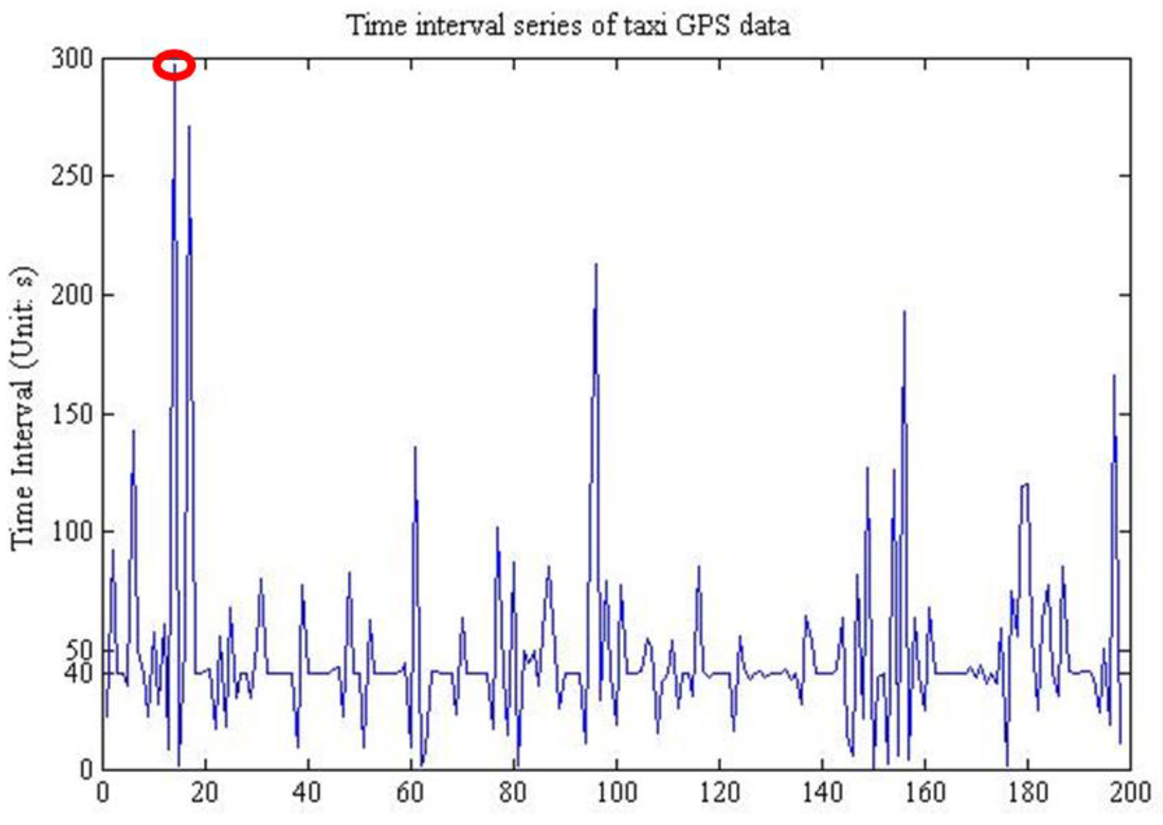
There are abundant kinds of sensors, which could be classified into three categories according to their observing frequency and data volume: low-frequency high-throughput sensors, such as satellite-borne sensors, by which data volume reaches Gigabytes with an observation a day or a month; high-frequency low-throughput sensors, such as soil moisture sensors, many in situ sensors belong to this type; high-frequency high-throughput sensors, such as video and camera sensor webs, due to their continuous observation and Megabyte-volume in seconds.

Based on the analysis above, this study, however, concentrates on the real-time data provision of the second type of sensors, which collect one data record with sub-kilobyte volume once an hour, a minute or a second. From the observing characteristics’ view, there are three kinds of data streams produced by this type of sensors. First is strictly steady data with little noise and the time interval is usually a constant value due to time-rigorous applications. Second is steady data whose time intervals can be changed as needed, but the observation intervals remain stable. Third is unsteady data influenced by too much noise, and the sample time stamps would have many changes, thus making numerous fluctuations to the time intervals between neighbor observations.

3. Method

3.1. Modeling the Provision Process

In this section, we model the data provision process considering that the time is discrete. We build a math description of the problem: with a historical time stamp series$\left[T_0,T_1,T_2,\dots ,T_n\right]$, $n$ is an integer, what the next time stamp $T_{n+1}$ is. To forecast or evaluate this value, we need to transform the problem first. We can get the time interval series $\left[𝛻t_1,𝛻t_2,𝛻t_3,\dots ,𝛻t_n\right]$ in which $𝛻t_k=T_k-T_{k-1}$, $k\in \left[1,n\right]$, if we could predict every next sleep interval $S{I}_{next}=𝛻t_{n+1}$, then $T_{n+1}=T_n+𝛻t_{n+1}$. As a result, $T_{n+1}$ can be computed by the forecast of the next SI. To better introduce this model, the meaning of some terminology used in this paper is shown in

Table 1. Meaning of terminology.

Phrases	Meaning
Delayed number (p)	The number of data items which are not accessed as the latest data.
Delay rate (D)	The percentage of delayed data items among total published data since the first request.
Miss hits (i)	The number of requests which fail to get new data published by SOS.
Waste rate (W)	The percentage of miss hits among all requests.
Time lag	The time interval between a successful request and the publishing of the latest data item.

. The data items, which are not accessed as the latest data are considered delayed in this paper.

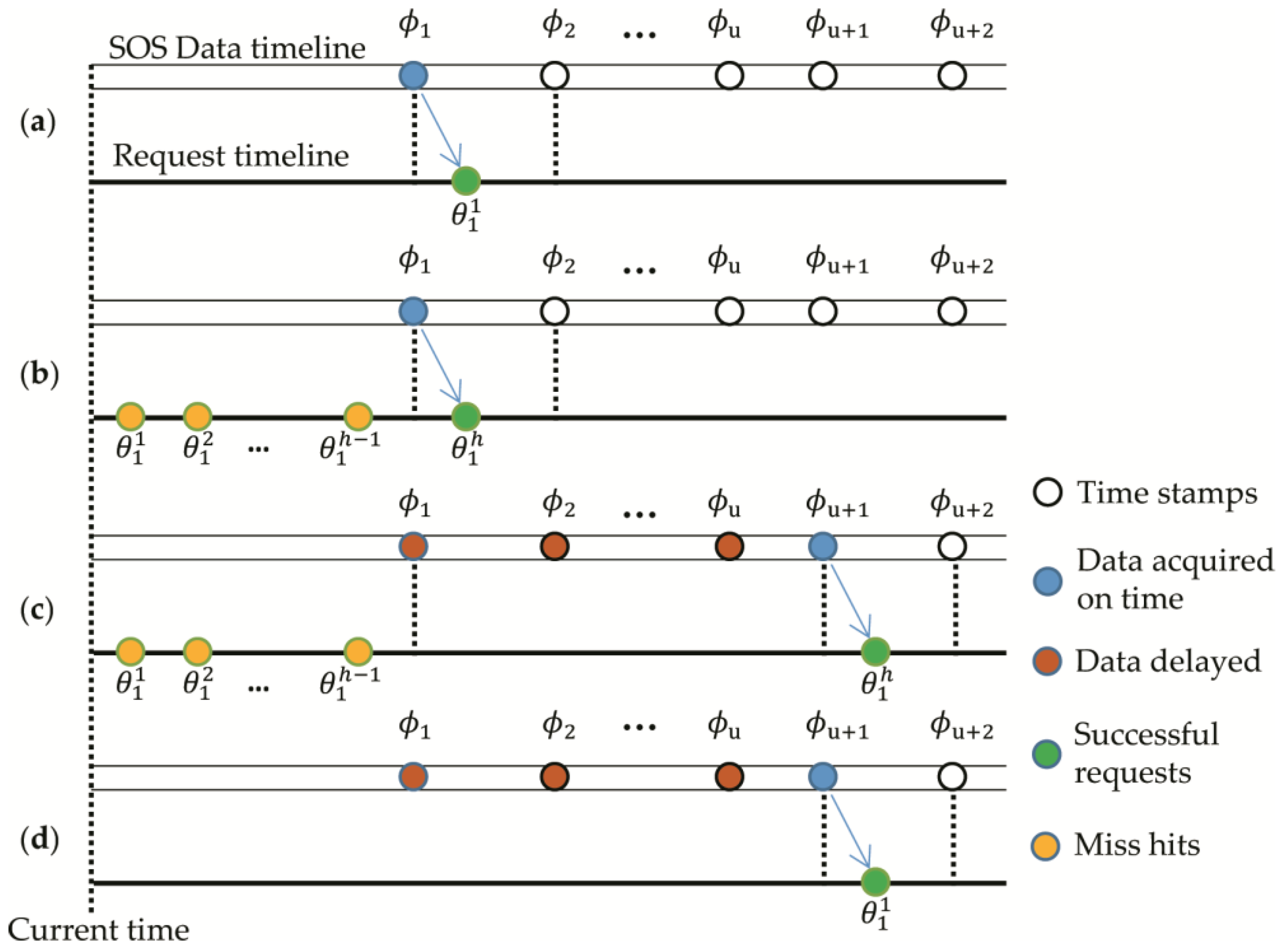
When the Harvestor starts to send data requests, the time stamps of the sensor data published by SOS can be defined as $\left[{\varphi }_0,{\varphi }_1,{\varphi }_2,{\varphi }_3,\dots ,{\varphi }_N\right]$, in which ${\varphi }_0=T_n, {\varphi }_1=T_{n+1}, {\varphi }_2=T_{n+2},\dots$, and $u$ is defined as the index of $\varphi$, $u\in \left[0, N-2\right]$. Through different provision algorithm $\Pi$, we could request the data produced at the time stamp ${\varphi }_1$ by a series of request time stamps [${\theta }_1^1, {\theta }_1^2, \dots , {\theta }_1^h$], in which $h \left(h=1, 2, 3,\dots \right)$ represents for the number of data request times, and the subscripts represent the index of$\varphi$. The delayed number of data is$p$, and the number of miss hits is$i$, all are integers, with a subscript $v \left(v=1, 2, 3,\dots \right)$ standing for the index of the data requested on time. In this case, $v=1$. There would be four cases shown in Figure 1, in which the corresponding explanations are as follows.

(a)

${\varphi }_1\le {\theta }_1^1<{\varphi }_2$, sensor data at time ${\varphi }_1$ is accessed from the first data request, with no delayed data or invalid requests, then $p_1=0, i_1=0$;

(b)

${\varphi }_1\le {\theta }_1^h<{\varphi }_2$, sensor data at time ${\varphi }_1$ has successfully been accessed after sending h times of data requests, with no delayed data and $h-1$ invalid requests, then $p_1=0, i_1=h-1$;

(c)

${\varphi }_{u+1}\le {\theta }_1^h<{\varphi }_{u+2}$, data at time ${\varphi }_{u+1}$ has been accessed after sending h times of data requests, the h − 1 requests for ${\varphi }_1$ have failed, while the hth request gets the ${\varphi }_{u+1}$ with data items ${\varphi }_1, {\varphi }_2,\dots , {\varphi }_u$ are delayed, then $p_1=u, i_1=h-1$;

(d)

${\varphi }_{u+1}\le {\theta }_1^1<{\varphi }_{u+2}$, data at time ${\varphi }_{u+1}$ is accessed from the first data request, with u data delayed and no invalid request, then$p_1=u, i_1=0$.

Based on the analysis of the requests for the first data item, it can be easily derived that in a common case, say the target data at time stamp ${\varphi }_v$ to be requested at time series [${\theta }_v^1, {\theta }_v^2, \dots , {\theta }_v^h$], we know ${\varphi }_{u+1}\le {\theta }_v^h<{\varphi }_{u+2}$, and$p_v=u, i_v=h-1$. Consequently, total miss hits ${\delta }_o\left(N\right)$ within which new data is not successfully acquired can be calculated by Equation (1), the total request number ${\delta }_d\left(N\right)$sent to SOS can be computed by Equation (2), the number of data delayed ${\epsilon }_o\left(N\right)$ can be a summation equation defined by Equation (3), and the total number of SOS data ${\epsilon }_d\left(N\right)$ is N as shown in Equation (4). V is the number of successful requests. Apparently, we could have an equation $V={\delta }_d\left(N\right)-{\delta }_0\left(N\right)={\mathsf{\epsilon }}_{\mathrm{d}}\left(N\right)-{\mathsf{\epsilon }}_0\left(N\right)$ to verify if the statistic numbers are right or not.

$${\mathsf{\delta }}_0\left(N\right)={\sum }_{v=1}^V{p}_v$$

(1)

$${\mathsf{\delta }}_{\mathrm{d}}\left(N\right)={\sum }_{v=1}^V{h}_v$$

(2)

$${\mathsf{\epsilon }}_0\left(N\right)={\sum }_{v=1}^V{i}_v$$

(3)

$${\mathsf{\epsilon }}_{\mathrm{d}}\left(N\right)=N$$

(4)

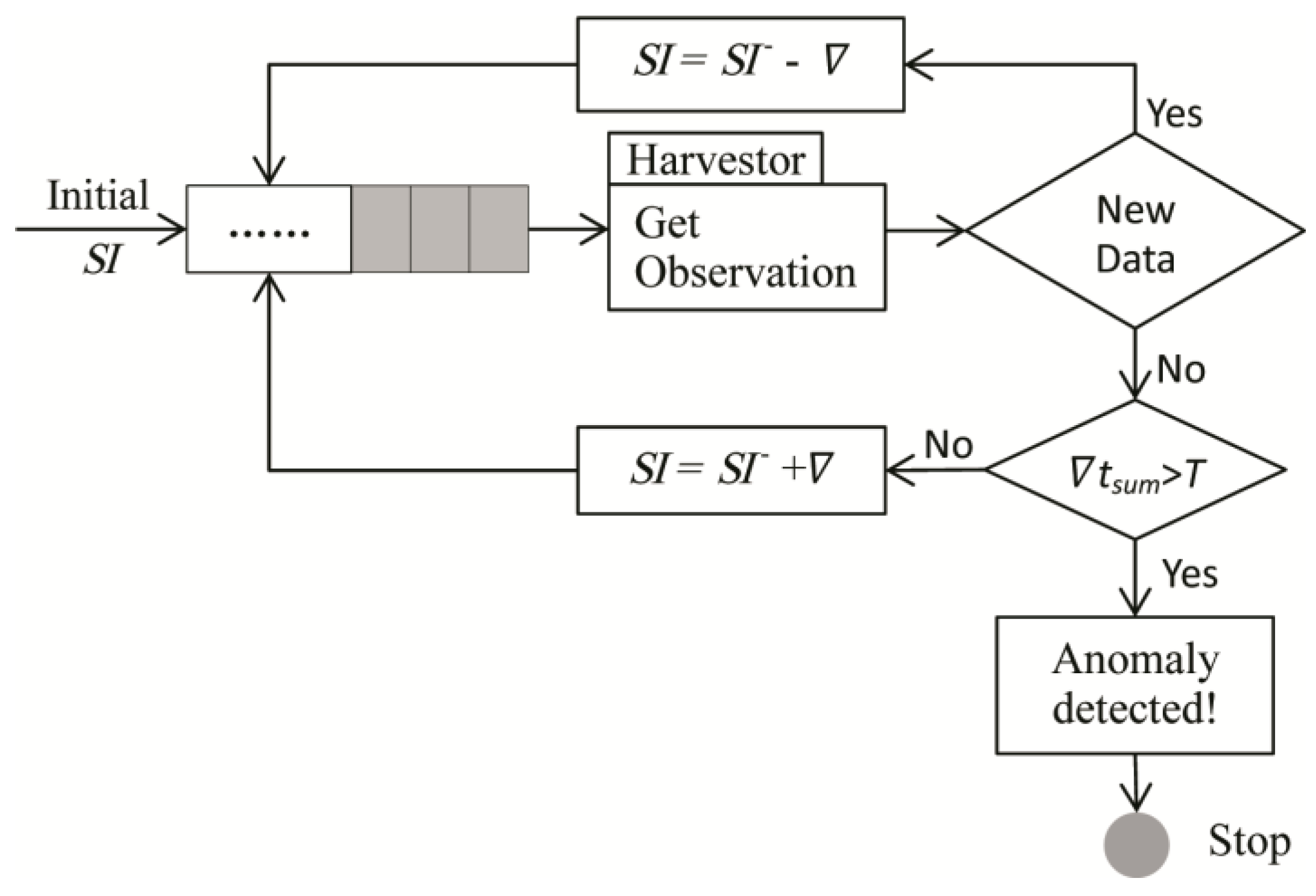
Based on the established model, the workflow is shown in Figure 2. SI represents for Sleep Interval, indicating the waiting time until a next data request, and SI⁻ represents for the last waiting time of the Harvestor. Harvestor is a function unit that actively collects sensor data by sending “GetObservation” request to the Sensor Observation Service (SOS). $𝛻$ is the adjusted time interval computed by different algorithms, while $𝛻$t_sum is the accumulative time in which new data cannot be acquired by several requests, and T is the maximum time threshold allowed to distinguish if there is an abnormal situation happens to the data provision of a specific sensor.

The model shown in Figure 2 depicts the provision process of how the system performs if the new data is successfully obtained or not. When the initial SI, namely the first waiting time, is finished, Harvestor sends a request to SOS to get a new data. If a new data is acquired successfully, then the next SI would be diminished a value$𝛻$, and if not, $𝛻$t_sum should be compared with T. If $𝛻$t_sum is larger than T, then the specific provision should be stopped, and, if not, the next SI should be increased by $𝛻$ to enter the next loop.

We need to announce two prerequisites of this study to exclude the influence of some unrelated factors since our concentration is the provision itself. First, we think that the data can be published on SOS and accessed immediately once it is produced by sensors, namely no time latency exists from the data is produced to it is published. Second, the time spent on data request and resolving response is so short relative to the whole process that it could be negligible.

3.2. Data Provision Methods

There are three kinds of time options for pull-based data provision to actively request sensor data [27], which is published by SOS. First is the Static Policy [17], in which way data are requested in a predefined fixed time interval; this algorithm will be stated in the Section 3.2.1. Second is the Instant Policy, with which once the system finished the current request, another request will be sent to SOS. This method is a kind of robbing access. We will discuss it in the Section 5. Third is the Adaptive Policy, by which the sleep interval is dynamically computed before every sensor data request. We describe three Adaptive Policies for data provision process: the Kalman Filter in the Section 3.2.2, and the Additive Increase Multiplicative Decrease for the Harvestor (H-AIMD) and Multiplicative Increase Additive Decrease for the Harvestor (H-MIAD) in the Section 3.2.3.

3.2.1. Static Policy

Static Policy is simply sending data request at a fixed time interval. The time interval could be set by two means. One is to be defined by users, in this way, the real-time performance is greatly influenced by the experience of the user. The other is the statistical learning of the historical time intervals. We could draw a histogram of the time intervals and select the peak value or pick the median value as the static time interval directly. After the decision of time interval SI, as shown in Figure 2, the adjust time interval $𝛻$ will have a permanent value 0, which means the Havestor will send a data request after every fixed time interval SI.

3.2.2. Kalman Filter

Kalman Filter (KF) [28] is a recursive analysis technique, which considers the process and measurement noise with estimation of time-dependent physical parameters. KF can provide the optimal state estimation when the noise model is accurate. Furthermore, it is efficient in computation and easily realized. All these advantages make it a very popular algorithm in control systems [23]. However, precise noise estimation is needed for KF if higher accuracy is desired. With these analyses, we consider using KF to evaluate the priori SI of the next state with the previous SI.

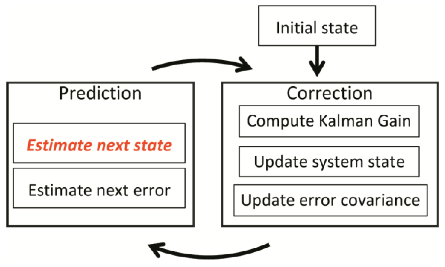
The workflow of KF is shown in Figure 3. It contains two main steps to perform the circulation. The first is the time update (prediction) and the second is the measurement update (correction). The prediction step is to evaluate the next state (seen the red words in Figure 3) and error propagation, with a corresponding Equation (5) to compute them. In this equation, $k$ is the discrete time slot index, with ${\widehat{x}}_{k-1}$ represents for previous evaluation state and ${\widehat{x}}_k^{-}$ is a primary estimate of current status (priori). $P_{k-1}$ is the error covariance matrix of the previous state, and $P_k^{-}$ is the priori estimate of the current error covariance matrix. $u_k$ is the control signal, and $A$ stands for state transmission matrix, $B$ is the control parameter matrix, and $Q$ is the process noise covariance matrix.

$$\{\begin{array}{l}{\widehat{x}}_k^{-}=A{\widehat{x}}_{k-1}+B{u}_k\\ P_k^{-}=A{P}_{k-1}{A}^T+Q\end{array}$$

(5)

After the system gets current measurement, KF goes to the second step, measurement update (correction), to update current measurement evaluation, shown in Equation (6). The Kalman Gain is represented by$K_k$, ${\widehat{x}}_k$ is the current state estimate (posteriori), $P_k$ is the error covariance. $R$ is the covariance matrix of measurement noise, $H$ is the transmission matrix to change from the state space to measurement space, $z_k$ is the measurement vector:

$$\{\begin{array}{c}{K}_k=P_k^{-}{H}^{\mathrm{T}}{\left(H{P}_k^{-}{H}^{\mathrm{T}}+R\right)}^{-1}\\ {\widehat{x}}_k={\widehat{x}}_k^{-}+K_k\left(z_k-H{\widehat{x}}_k^{-}\right)\\ P_k=\left(I-K_{k}H\right)P_k^{-}\end{array}$$

(6)

The KF iteration starts from the$k=0$, when the $x_0 \text{and} P_0$ is provided as the initial state. Then, we could begin with the iteration, which uses the estimation of the previous state ${\widehat{x}}_k^{-}$ and $P_k^{-}$ as input to get a priori estimation for the current state. After that, the measurement update equation set is used to get the estimation value ${\widehat{x}}_k$ of $x$ at time slot $k$, which will be used for the next iteration.

We adapt the KF algorithm as a one-dimensional solution for our proposed model and then preset the corresponding parameters. In this study, $k$ is seen as the index of data items published by SOS. First, we set the primary state as $P_0=1$ and the initial time interval as the median value of history intervals, namely $x_0=\text{Median}\left(𝛻t_1,𝛻t_2,𝛻t_3,\dots ,𝛻t_n\right)$. No control signal is in the provision process, so $u_k=0$. Accordingly, we do not need to consider the value of B any more. The noise parameter $Q$ and $R$ are defined as the variance of the historical time interval series, so they can be computed by Equation (7), in which $n$ is the number of time intervals. In our one-dimensional problem, no transition is needed between the state space and measurement space, so $A \mathrm{and} H$ are both constant 1:

$$Q=R=\frac{1}{n-1}{\displaystyle \sum }_{l=1}^n{\left(𝛻t_l-\frac{1}{n}{{\displaystyle \sum }}_{l=1}^n𝛻t_l\right)}^2$$

(7)

3.2.3. H-AIMD and H-MIAD

A global algorithm Energy Balancing Correlation-dependent Wakeup (EB-CW) for the sensor recharge scheme was suggested to determine the relationship between the dynamic process of rechargeable sensor nodes and the event occurrence [25]. EB-CW can achieve optimal performance if the global parameters, like the energy quantity of sensor charge and discharge process, and probabilities of the next state, are known. However, we could not get the global parameters in most cases. Then, the local algorithm AIMD [20] was introduced to the sensor recharge sensor node activation to determine the status and parameters of sensor nodes dynamically, including activation, sleeping, and sleeping time intervals.

We borrow insights from AIMD and use it in the provision process of sensor data instead of its original application in network congestion [29] and sensor recharge [20,24,26] studies. The modified algorithm H-AIMD, in which “H” represents the Harvestor, is introduced for SI computation. Similarly, we also describe the H-MIAD in this section and will perform the experiments on them in Section 4, due to the huge performance difference between the algorithm AIMD and MIAD, found in [24].

The detailed steps of H-AIMD are shown in Algorithm 1. If the Harvestor does not get new data, then additively increase SI with the value$c_1, c_1>0$; and if it does, then multiplicatively decrease SI with the value$c_2, c_2>1$. The determinant condition of H-AIMD is if the Harvestor gets new data or not, which is more simple than the threshold comparison of the AIMD used for sensor activation process. Considering many studies that have verified that when$c_1=1, c_2=2$, the performance is the best [24,30], we use the same parameter setting in this study. Moreover, since the Harvestor could easily get the acquired values (getNewData, SI_prev) as inputs, this algorithm is extremely easily realized in practice.

Algorithm 1 Adaptive Computing SI Through H-AIMD
1.	Input: getNewData, SIprev
2.	Output: SInext
3.	If getNewData = false then
4.	SInext = SIprev + c1
5.	else
6.	SInext = SIprev/c2
7.	end if
End Algorithm

Similarly, H-MIAD is derived from the algorithm Multiplicative Increase and Additive Decrease (MIAD) and used in the Harvestor data provision. If the Harvestor does not get new data, then SI_next = SI_prev × c₁, $c_1>1$; and if it does, then SI_next = SI_prev − c₂, $c_2>0$. In this study, we define $c_1=1.1, c_2=1$.

3.3. Performance Evaluation

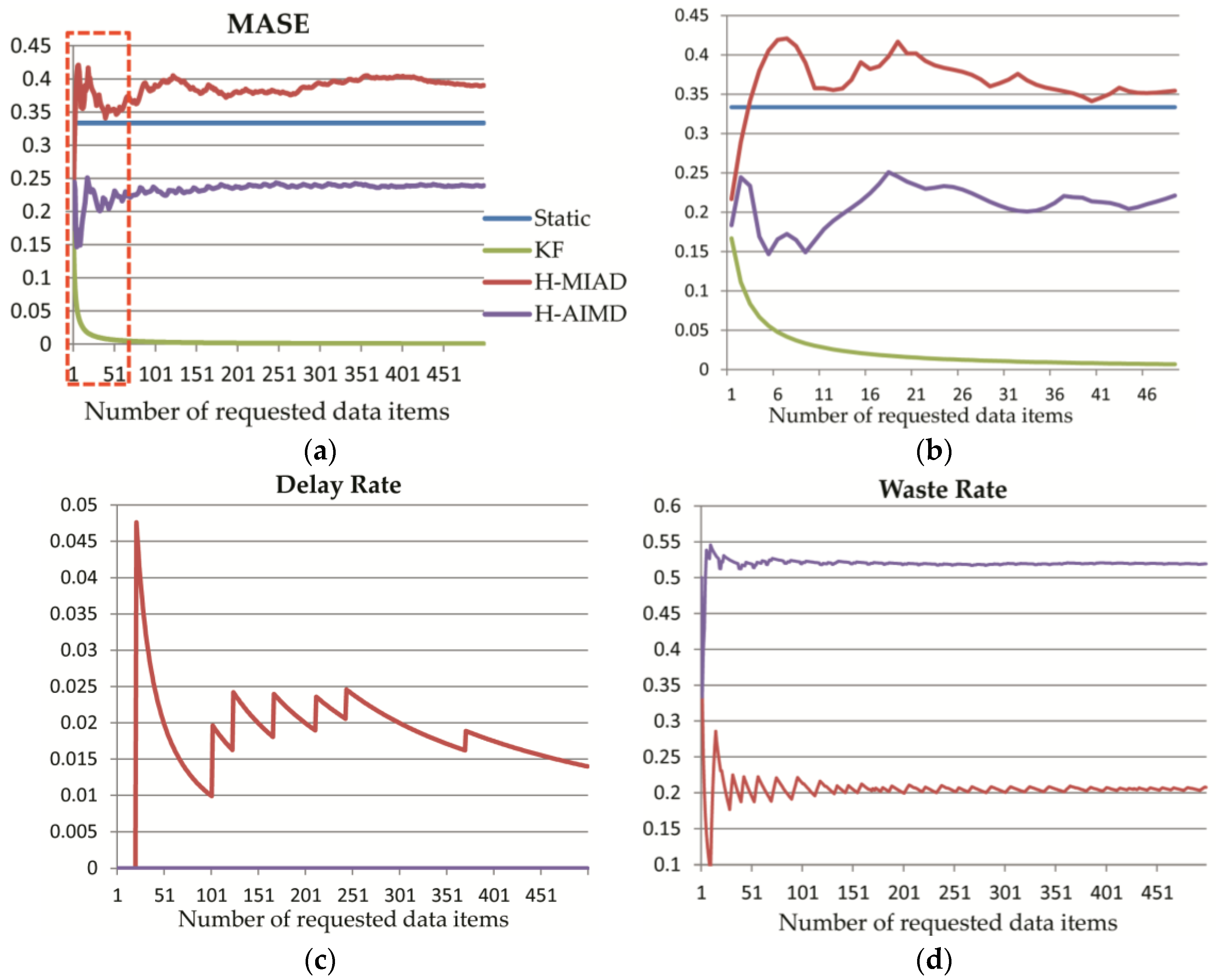
In this study, we define a comprehensive performance evaluation$P=\text{Function}\left(E, D,W\right)$, taking three factors into account. First is the accuracy of SI_next (E), which indicates the accuracy of forecast time stamps. Second is the delay rate of data (D), which is also a key consideration in many applications; and third is resource waste (W), which is an element under consideration for redundancy. In addition, in order to realize the properties of the equilibrium, it must be avoided that the value of one factor is so large that it suppresses the others or too small in the assessment. Under this condition, we think the evaluation method should be normalized so that different algorithms could be compared in different applications. In this section, each of these factors will be defined under these considerations.

To evaluate the SI error, the Mean Absolute Scaled Error (MASE) [31] is used, and computed by Equation (8). E is the evaluation error, $Y_t$ is the observation at time slot t, $F_t$ is the forecast, and N is the number of data items. Different from the Root Mean Square Error (RMSE), MASE is scale independent, which is very suitable for error comparison between different applications. Specially, MASE is usually less than 1 if the forecast error is less than one step of the data series, namely $E\in \left[0, 1\right]$, otherwise $E=1$. In this study, the t, i stand for time interval indexes instead of time slots.

$$E= \frac{{{\displaystyle \sum }}_{t=1}^N\left|Y_t-F_t\right|}{\frac{N}{N-1}{{\displaystyle \sum }}_{i=2}^N\left|Y_i-Y_{i-1}\right|}$$

(8)

The second factor is the data delay rate $D(\Pi )$. Under data provision algorithm $\Pi$, it can be computed by Equation (9). The total number of SOS data ${\epsilon }_d\left(N\right)$ and the number of data delayed ${\epsilon }_o\left(N\right)$ can be acquired by Equations (3) and (4), respectively. Apparently, $D(\Pi )\in \left[0,1\right],$

$$D\left(\Pi \right)= \underset{N\to \infty }{lim}\frac{{\epsilon }_o\left(N\right)}{{\epsilon }_d\left(N\right)}$$

(9)

The third factor is the miss hit rate $W(\Pi )$, which can be acquired according to Equation (10) under the data provision algorithm $\Pi$. The total request number ${\delta }_d\left(N\right)$sent to SOS can be computed by Equation (1), total waste requests in which new data is not successfully acquired ${\delta }_o\left(N\right)$ can be calculated by Equation (2). We can conclude that $W(\Pi )\in \left[0, 1\right)$.

$$W(\Pi )= \underset{N\to \infty }{\lim }\frac{{\delta }_o\left(N\right)}{{\delta }_d\left(N\right)}$$

(10)

$$\{\begin{array}{c}P=1-\left({\omega }_1\times E+{\omega }_2\times D+{\omega }_3\times W\right)\\ {\omega }_1+{\omega }_2+{\omega }_3=1\end{array}$$

(11)

With all the factors defined, the weighted normalized performance evaluation model can be calculated by Equation (11), in which ${\omega }_1$, ${\omega }_2$, ${\omega }_3$ are all weight coefficients and no less than 0. Because $E\in \left[0, 1\right], D(\Pi )\in \left[0, 1\right], W(\Pi )\in \left[0, 1\right), \text{and} {\omega }_1\in \left[0, 1\right]$, ${\omega }_2\in \left[0, 1\right]$, ${\omega }_3\in \left[0, 1\right]$, we can get ${\omega }_1\times E\in \left[0, {\omega }_1\right], {\omega }_2\times D\in \left[0, {\omega }_2\right], {\omega }_3\times W\in \left[0, {\omega }_3\right)$, then $\left({\omega }_1\times E+{\omega }_2\times D+{\omega }_3\times W\right)\in \left[0, {\omega }_1+{\omega }_2+{\omega }_3\right)=\left[0, 1\right)$. Therefore, P ∈ (0, 1], thus the performance is scale independent. Owing to this normalized equation design, the performance of different algorithms can be compared in one application and the same algorithm can also be compared in different applications.

4. Experiments and Results

This study considered three real sensor data environments including methane concentration of WangJiaLing coal mine in Shanxi Province, BaoXie soil moisture and Wuhan taxi GPS records in Hubei Province, all in China. The first two are in situ sensors, while the third is mobile sensor data. In this section, experiments of the four algorithms described in Section 3.2 will be performed in these environments. In addition, the results of time efficiency, delay rate, and waste rate are shown in figures and listed in tables.

4.1. Gas Concentration of a Coal Mine

Methane is a highly explosive gas trapped within coal layers [3]. When the concentration of the gas reaches to some extents, fatal asphyxiation and explosive risk become significant. Thus, uninterrupted monitoring is vital [3]. Therefore, gas sensors have very stable power supply and are able to get observations in very stable time intervals. The test data used in this section come from the gas sensors deployed in the WangJiaLing coal mine, with static monitoring frequency 30 s/record. With these data, two experiments are performed on 500 records.

The first test is performed on the relationship between the initial provision time lag and the performance factor MASE of four algorithms, shown in Figure 4. The Kalman Filter (KF) has the lowest MASE values, less than 0.001, which are very close to zero and make the line coincide with the x-axis. H-AIMD is also very stable and has lower MASEs than that of H-MIAD, whose line has more fluctuations. At mean time, the line of Static Policy is linearly increasing with the time lag increases. It indicates that the time lag of the first data item influences the performance of the Static Policy greatly.

After the initial time lag test, the influence of increasing number of requested items is also inspected on the performance factors between the four algorithms with an initial time lag 10 s, as can be seen in Figure 5. Figure 5a represents the variation of MASE with the number of requested data items and Figure 5b enlarges the part of the first 50 data items in (a). These two subplots show that the Static policy has a constant MASE value 0.33, while after some fluctuations, the value of H-AIMD converges to about 0.25, less than the Static Policy. The value of KF has slowly decreased to a value very close to 0 around the 50th data item. This is due to the 10 s time lag of the first data item, the MASE is 0.17, but since the second data request, KF can predict a very accurate time interval with the parameters computed through Equations (5)–(7), thus leading to a continuous decreasing with more data requests. In addition, H-MIAD is not only unstable but also has a rather higher MASE than the other policies, and it also has a delay rate while the others are equal to 0, observed from Figure 5c. Figure 5d illustrates that the waste rate of H-AIMD is rather high with a stable value around 0.52, and that of the H-MIAD is about 0.2. The waste rate of Static and KF equals 0, which means they have no invalid requests in this experiment.

4.2. Observations of Soil Moisture

The sensors which observe soil moisture are deployed outdoors for modern agriculture [4], usually charged by solar energy. At daytime, if it is sunny or daylight is very adequate, the power absorbed by the solar battery is sufficient for the sensors to work. Otherwise, if it is nighttime or it is rainy or cloudy, the energy cannot support continuous observations. Thus, it leads to a long-term pause without data records. Because this kind of application is not time strict, the frequency is low in general. In this study, the data of a soil moisture sensor deployed in Baoxie, Hubei Province, China, has 4554 records in one year starting from January 2014 to January 2015. The time unit is min.

Part of the sample data is shown in Figure 6. It can be concluded from the figure that the stable time interval is 60 min with some fluctuations, most of which are below the stable line 60 min. For example, data marked by a red rectangle show regular fluctuations, which could be caused by some artificial operations, while others without obvious patterns are very likely caused by the environmental noise. The time interval marked by a little red circle, however, is 3668 min, about two and a half days, which is much larger than the normal value of 60 min. This situation may be produced by the severe weather or a machine breakdown. In this section, the median time interval 60 min was used as the initial SI, which is provided as priori value for the Static Policy.

With this data, we test the algorithms and get the performance values, shown in

Table 2. Performance of Different Algorithms (the unit of Mean Absolute Scaled Error (MASE) is min).

Performance Factors	Static	Kalman Filter	H-MIAD	H-AIMD
MASE	0.1119	0.2251	0.7755	0.0512
Delay Rate	23.96%	70.02%	87.92%	4.02%
Waste Rate	60.22%	48.65%	55.32%	69.25%

. It can be seen that the data Delay Rate and MASE of H-AIMD is extremely low and much less than the others. In contrast, the extremely high data Delay Rate makes H-MIAD and KF unsuitable for this kind of data provision. The Static policy, however, has a relatively low MASE and Delay Rate.

4.3. Urban Taxi GPS Data

As one of the most important transportation tools, taxis, attached with GPS devices, have become an important data source for many applications, such as data mining, road planning, and transportation infrastructure building. The data collected by GPS instruments, then, are transmitted to the traffic center for real-time monitoring. It should be noticed that the GPS signals are slightly affected by the environments, for example, the high building and bridge openings, or no data for a relatively long time if the drivers are taking a rest, having their meals, or waiting for passengers. In the experiment of this section, we use the 1309 GPS data records of a taxi in one day in Wuhan City, Hubei Province, China.

Sample data intervals are seen in Figure 7, showing the time interval characteristics of the taxi GPS data. We find that there is a stable time interval 40 s, while there are also many fluctuations that are caused by the environment and the driving experience of the drivers. Then, if having a look at the point, which is marked by a little red circle, it indicates about a five-minute time interval. This situation happens so often because the driver should wait for passengers now and again. Furthermore, we have also found a time interval showing no observation in about five hours, which may be caused by the car inspection and maintenance or a rest of the driver. In this study, the median time interval 40 s was used as the fixed time interval for the Static Policy.

With this mobile sensor data, we performed the performance test of the four algorithms on data provision, shown in

Table 3. Performance of Different Algorithms (the unit of Mean Absolute Scaled Error (MASE) is s).

Performance Factor	Static	Kalman Filter	H-MIAD	H-AIMD
MASE	0.1669	0.2856	0.1090	0.0771
Delay Rate	12.07%	22.77%	22.38%	0.76%
Waste Rate	47.20%	30.19%	66.74%	67.16%

. We find that like the results shown in Section 4.2, the H-AIMD also has the lowest Delay Rate, and MASE, although its Waste Rate is relatively high. Similarly, the Static Policy has relatively lower values of those factors than KF and H-MIAD. The Kalman Filter, however, shows the worst MASE and Delay Rate in this experiment due to its excessive sensitivity to the fluctuations.

5. Discussion

In this section, the advantages and disadvantages of the provision methods are discussed first, followed by the application situation of our model and the performance evaluation method. After that, comparison of the four algorithms in real sensor data provision experiments is made with the performance data from Table 1 and Table 2. Then, a detailed cause of influence analysis on the performances is made. Afterwards, we discuss the different applicable conditions of the algorithms in high-frequency sensor environments.

Concerning the provision methods, we could choose the Instant Policy, by which the latest data are supposed to be acquired immediately after the previous request, which is mentioned in Section 3.2. Obviously, this way has an utmost real-time efficiency but the extremely high frequency may lead to huge resource waste. Worse still, it will largely increase the load of SOS data servers, which would lead to low response during huge parallel data access, thus decrease its efficiency in reverse. Furthermore, some sensors would change their observation frequency according to some conditions, such as human control, low energy supply, or self-adaptive monitoring of the environment. Therefore, to minimize a delayed number of data, relief both of the workload of the data server and Harvestor, and efficiently acquire the latest data, the Static Policy and other self-adaptive algorithms would be preferable.

We proposed a provision model to analyze the real-time problem of the widely used pull-based data access method for the sensor observation services of sensor webs. This model focuses on data provision of a single sensor, but it can be easily used for a large number of sensors, cooperating with the flexible provision management mechanism introduced by our previous work [27,32]. It is a kind of batch processing method with which data of every single sensor is requested independently as a pipeline configured and managed by a control unit. Based on the mechanism and our proposed model, a taxi company can handle the data provision of thousands of cars with sufficient hardware support, although only one taxi data was used to test the real-time performance of the four policies in Section 4.3. In addition, this model is not only suitable for sensor webs but also be used to other pull-based real-time data acquisition.

Upon the mathematical model, three performance evaluation factors are also put forward. MASE, which is scale independent, shows the forecast error of time intervals. Both MASE and Delay Rate imply the efficiency of different policies. Resource Waste denotes the percentage of redundancy data requests, namely, the invalid resource usage. The weights of the three factors shown in Equation (11) can be flexibly set in different applications to guarantee the highest time efficiency with the lowest Resource Waste. Based on this consideration, we did not compute the comprehensive performance in Section 4. However, the normalization design makes these evaluation factors very adaptive for performance comparison between different policies or same policy between different applications.

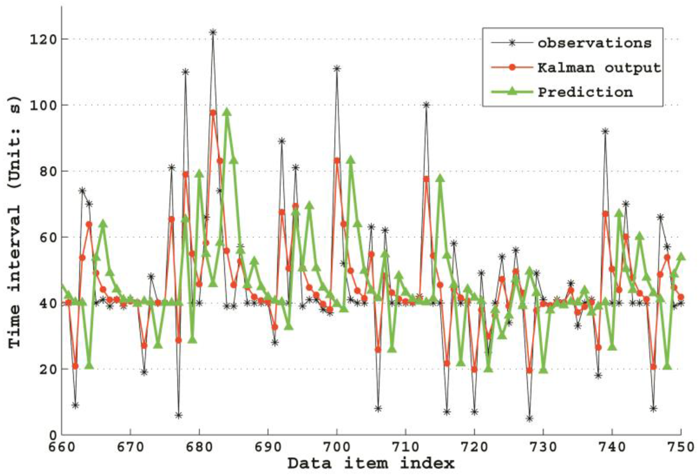
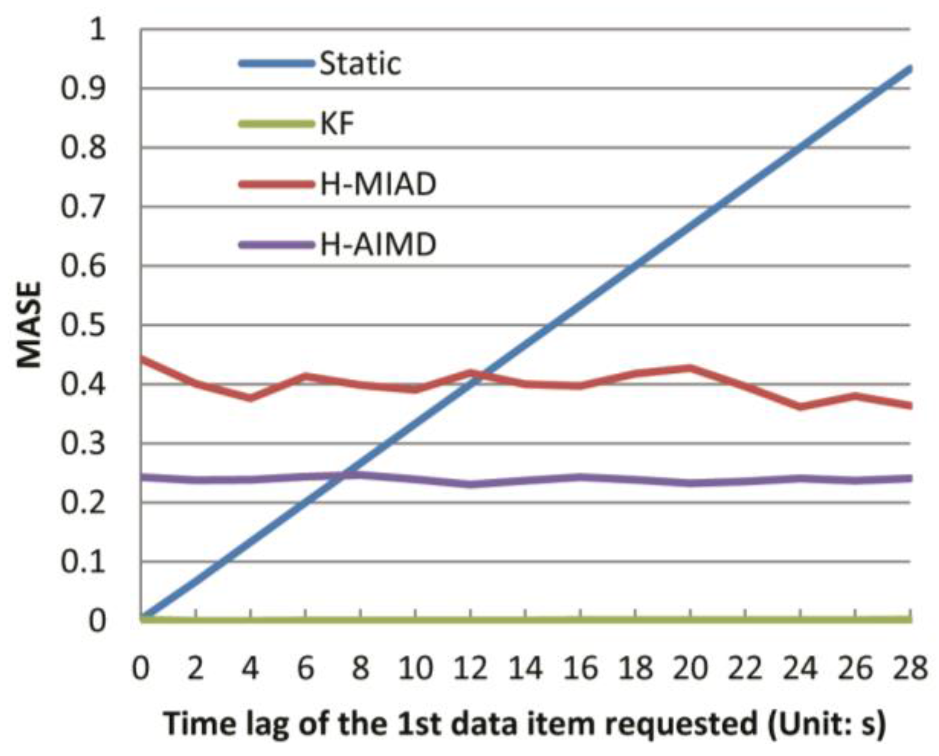
The Kalman Filter has a very high performance in a stable time interval application. It is because that the KF algorithm could gradually converge to true values, while in the other two applications, its performance is not ideal for the reason that accurate noise model cannot be acquired, then it will produce huge errors with the priori evaluation of current state as the forecast value. Let us take a deeper look at the KF forecast mechanism in Figure 8, which shows a sample fragment of GPS time intervals, with Kalman priori predictions (green line) and posteriori correction output (red line). According to the parameter settings in Section 3.2.2, in this study, the priori forecast values are equal to the posteriori of previous state value. In Figure 8, if moving the red line along x-axis for one step, we can get the green line. Therefore, we could conclude that the reason why the performance of the KF algorithm is not so ideal in the latter two experiments is that we could not estimate the noise accurately, which makes the forecast error very high. With these analyses, it can be easily understood that the KF algorithm has low time forecast accuracy, leading to a high delay rate in applications with many time interval fluctuations produced by environment noises. However, in fixed time interval applications, its performance can gradually converge to optimum even with a poor initial value. Therefore, the KF algorithm is suitable for a long-term sensor data provision with relatively stable time intervals.

We proposed the H-MIAD and H-AIMD, borrowing insights of network congestion algorithms MIAD and AIMD. Shown by the experiments in Section 4, the H-AIMD is very stable and high overall performance under various kinds of sensor data applications. As a whole, the H-AIMD gets high real-time efficiency and low delayed number of data by increasing the data request frequency, thus leading to more resource waste. In contrast, the performance of H-MIAD is too low to be used for data provision. This finding matches the previous work on the theoretical identification of the algorithms MIAD and AIMD, which discovers that the AIMD is very stable while the MIAD is an unfavorable algorithm [24].

With the analysis of the algorithms above, it can be drawn that the algorithms can be suitable for different kinds of applications. If a sensor has a strict-fixed observation time interval and every time stamp can be easily and accurately deduced, then there is no need to perform dynamic provision algorithms since the Static Policy would have a perfect performance in this situation. Actually, the Static Policy needs accurate priori parameters. When the time interval is very stable with some adjustments now and then, the recursive algorithm KF can offset the change and gradually converge to the new value. Thus, the KF has perfect performance in this condition. The linear algorithm H-AIMD, in contrast, has a more stable and higher performance than the others when there are much unclear environmental noises. Apparently, the algorithms KF and H-AIMD can dynamically adjust time interval according to varying states, and no precise priori value is desired.

6. Conclusions

Commonly used sensor web service standards for data access are pull-based, which cannot ensure the real-time efficiency. We modeled the process of real-time sensor data provision, proposed three self-adaptive dynamic provision algorithms, and compared them with the Static Policy with three suggested performance evaluation factors in this study. Our model is suitable for real-time geographical information platforms, and the performance evaluation method is also feasible for not only different algorithms in the same application but also the same algorithm in different applications. However, there still are some concerns for our future work. Since we only refer to literature to set the parameters of H-AIMD algorithm in this paper, a more detailed analysis and sufficient experiments on real sensor data will be performed to explore the optimal settings of those parameters in the future. More possible algorithms could also be introduced in this model.