Article

Lane-Level Road Information Mining from Vehicle GPS Trajectories Based on Naïve Bayesian Classification

1
State Key Laboratory of Information Engineering in Surveying, Mapping, and Remote Sensing, Wuhan University, Wuhan 430079, China
2
Shenzhen Key Laboratory of Spatial Smart Sensing and Services, College of Civil Engineering, Shenzhen University, Shenzhen 518060, China
*
Author to whom correspondence should be addressed.
ISPRS Int. J. Geo-Inf. 2015, 4(4), 2660-2680; https://doi.org/10.3390/ijgi4042660
Submission received: 16 June 2015 / Revised: 11 November 2015 / Accepted: 17 November 2015 / Published: 26 November 2015

Abstract

:
In this paper, we propose a novel approach for mining lane-level road network information from low-precision vehicle GPS trajectories (MLIT), which includes the number and turn rules of traffic lanes based on naïve Bayesian classification. First, the proposed method (MLIT) uses an adaptive density optimization method to remove outliers from the raw GPS trajectories based on their space-time distribution and density clustering. Second, MLIT acquires the number of lanes in two steps. The first step establishes a naïve Bayesian classifier according to the trace features of the road plane and road profiles and the real number of lanes, as found in the training samples. The second step confirms the number of lanes using test samples in reference to the naïve Bayesian classifier using the known trace features of test sample. Third, MLIT infers the turn rules of each lane through tracking GPS trajectories. Experiments were conducted using the GPS trajectories of taxis in Wuhan, China. Compared with human-interpreted results, the automatically generated lane-level road network information was demonstrated to be of higher quality in terms of displaying detailed road networks with the number of lanes and turn rules of each lane.

1. Introduction

Accurate lane-based road network data for navigation, such as lane location, lane changes, and turn information, is crucial for ensuring reliable and safe driving, especially for intelligent transportation systems (ITS) such as advanced driver assistance systems and autonomous driving. In addition, lane geometry information, especially the number of lanes, can also be important for inferring the type of road and for estimating traffic flow capacity. Conventional road networks, which are extracted by digitization, mobile mapping vehicles, or aerial photographs, are based on road centerlines [1,2]. Lane-level information (such as number of lanes and turning in the intersection) is usually acquired from high-definition video/images, laser point clouds, or DGPS/INS trajectories [3,4,5,6,7]. Mining such detailed information is time consuming and labor intensive [8].
Increasingly, public vehicles and personal navigation assistants are equipped with single-frequency global position system (GPS) trackers or loggers that monitor the user locations at regular intervals [9,10]. The quality of tracking data is often low due to the geometrical effects of urban canyons on the accuracy of GPS ranging, thereby causing tracking points to deviate from the original roads. However, large volumes of data can be inexpensively acquired using GPS tools. This new type of geospatial resource contains abundant information regarding road networks, traffic conditions, points of interest, and driving behaviors [11,12,13]. Extracting high-quality road maps from low-quality tracking data is a hot topic [14,15,16,17]. As compared to the existing approaches for generating lane-based network information, a geospatial approach takes full advantage of information generated by spatial and temporal tracking data, thus enabling a user to establish or update road networks (e.g., road-level network and lane-level network) in relation to traffic rules.
This study proposes an approach (MLIT: mining lane-level road network information from vehicle GPS trajectories) to automatically generating lane-level road information including number of lanes and intersection turns from low-precision vehicle GPS trajectories gathered from thousands of taxis in a city. To reduce the impact of low accuracy and other vagaries in taxi trajectories, we take steps to offset the uncertainty of lane-based road network extraction. First, trajectories gathered in off-peak times comprise the experimental data [18,19]. Second, segmentation treatment is adopted during optimization and lane information extraction to avoid the significant impact of large vibrations on the spread of trajectories due to the changes in traffic features such as uncertain traffic flows and lane additions at different positions on the same road. Therefore, we define the trajectory segment section (TSS) as the basic unit for trajectory optimization and lane information extraction. Specifically, according to the trace features of the road plane and road profile, and the real number of lanes found in the training samples, we construct a naïve Bayesian classifier to infer the number of lanes from the test samples based on these trace features. The turn rules of each lane, including going straight, or making a left, right or U-turn, are extracted by tracking trajectories in relation to the rate of reckless driving. The contributions of this paper are as follows:
(1)
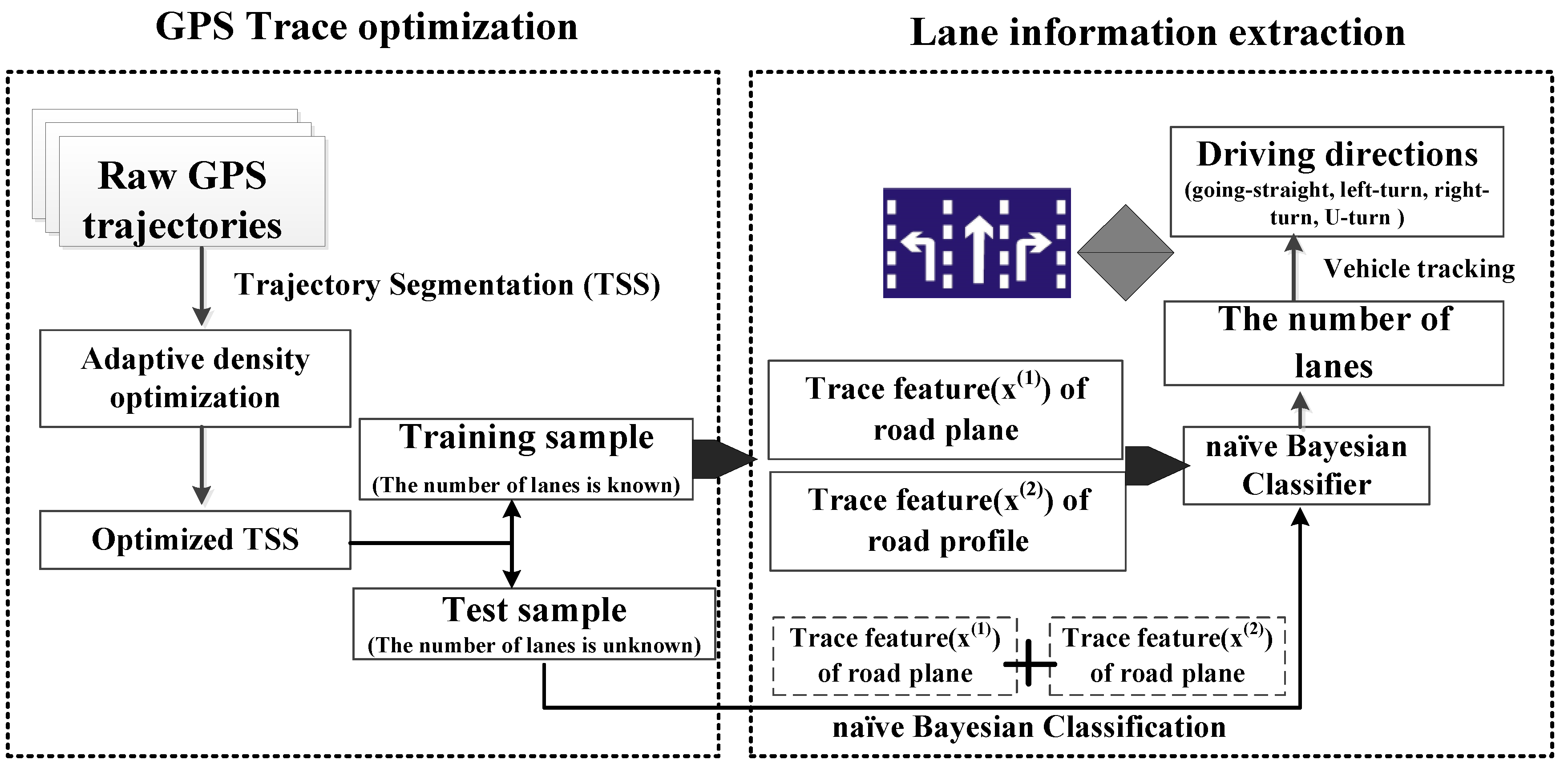
We propose a new method, the adaptive density optimization method, for vehicle GPS trajectory optimization based on the density clustering method and the spatial distribution of tracking points. Outliers mixed in the raw data are removed automatically using adaptive density optimization method.
(2)
We explore a novel way to infer lane-level information from low-precision spatiotemporal vehicle GPS trajectories (MLIT).
(3)
We detect turn rules of each lane by tracking vehicle trajectories in relation to the rate of reckless driving.
The remainder of this article is organized as follows. In Section 2, related studies on outlier removal and extracting lane information from low-precision GPS trajectories are reviewed. In Section 3, we fully describe the proposed method for detecting traffic lane information. In Section 4, a series of experiments on Wuhan datasets demonstrate the advantages and effectiveness of the proposed method. In Section 5, the conclusions and directions of future research are discussed.

2. Related Work

Spatial trajectories are never perfectly accurate, due to sensor noise and other factors. Sometimes the error is acceptable, such as when using GPS to identify the city where a person is located. In other situations, various methods to remove noise and decrease the error in the measurements are applied to trajectory data. Specifically, trajectories gathered by public vehicles include massive amounts of real-time and low-cost information (e.g., road network, point of interests, driving behaviors). This information also contains many outliers due to the limitations of the collection equipment, the environment, and purpose. The main categories for outlier removal include filtering algorithms to smooth the noise, map-matching methods to change the original coordinates of tracking points to fit them to the existing road network, and clustering methods to remove outliers.
Filtering is important when the trajectory data is particularly noisy, or when it is necessary to derive other quantities like speed or direction from these data. In addition, filtering is suitable for trajectories with high sampling frequency only. Lee in [20] gave a detailed introduction on how to implement a filtering algorithm, including the Kalman filter and particle filter. Another pre-processing step uses map-matching methods to match the trajectories to the road network. Sotiris Brakatsoulas [21] presented three map-matching algorithms that focus especially on the trajectory nature of the data rather than simply on the current position, as in traditional map-matching techniques. It is important to note that map-matching methods apply only to road-level information extraction from GPS data because each tracking point is matched to the centerline of the carriageway, and its original location is changed. In contrast to these methods, some researchers have used clustering for outlier removal. For example, Jing Wang [15] proposed using kernel density methods to remove outliers among raw GPS trajectories. Chen [7] sorted all the data points in ascending order according to their distances from the median and then chose 95% of the sorted data points as the experimental data. Compared with filtering techniques and map-matching methods, clustering methods do not change the position of tracking points, and are less susceptible to sampling intervals, making them most suitable for outlier removal when dealing with a large volume of low-quality GPS trajectories at a low sample frequency and affected by urban canyons. However, in our case, the experimental data is collected in an urban area and their position accuracy and sampling rate are about 10–15 m and 20 s respectively. The kernel density estimation with a fixed bandwidth for outlier removal is not suitable for a complex road network in an urban area. In addition, the outlier’s proportion of low-precision GPS data far exceeds 5%. Therefore, we are motivated to use an adaptive density estimation method to remove outliers.
After data pre-processing, automatic road network refinement from GPS trajectories becomes possible. OpenStreetMap employs user-contributed GPS trajectories to create free digital maps that are open for editing by registered users [22]. Likewise, WikiMapia, Google Maps, and other map applications let users update maps. There has also been work on completely automated methods to infer road maps fromlow-quality GPS trajectories. Those methods include matching GPS traces to prototypical shapes [23], using incremental methods to process GPS traces and generate road maps [24,25], and applying clustering methods or artificial algorithms to extract road networks from GPS traces [26,27,28]. According to the references [23,24,25,26,27,28], the existing methods can generate and update road-level maps from low-quality vehicle GPS trajectories, while latter studies addressing detailed road network generation have gradually shifted down to lane-level road network information.
Lane-level information extraction from vehicle trajectories starts with high-precision differential GPS data and concludes with a refinement of an existing map, including locating lanes and number of lanes [29,30]. This process involves smoothing and filtering the GPS data, matching it to an existing map, spline fitting the road centerline, clustering to find lanes, and refinement of the intersection geometry. Uduwaragoda [31] proposed using high-precision vehicle trajectories collected by vehicles equipped with INS/GPS-enabled mobile phones to generate lane-level road maps based on kernel density estimation. However, the methods proposed in [29,30,31] are based on the assumption that GPS traces from different lanes are separated well. For low-precision GPS data, this assumption is seriously violated, and therefore a kind of probabilistic method with prior knowledge is used to extract lane structure from a mass of low-precision GPS trajectories. Moreover, previous study [31] did not consider detailed lane extraction across large areas or regions, nor did it focus on turn extraction. Our study contributes to the existing research not only by generating lane-level road network information, including the number and turn rules of traffic lanes from pre-processing low-precision vehicle GPS trajectories, but also empirically evaluating the validity of the results for large areas and regions.

3. Lane-Level Road Network Information Extraction from Vehicle GPS Trajectories

In this section, we present the lane-level road network information (e.g., number of lanes and turns of each lane) extraction method (MLIT) from low-precision GPS trajectories. The architecture is shown in Figure 1. The processing of MLIT is described as follows:
First, outliers in each TSS (trajectory segment section) are removed automatically with the adaptive density optimization algorithm.
Second, a naïve Bayesian classifier is constructed by analyzing the trace feature (x(1)) of the road plane and trace feature (x(2)) on the road profile and the real number of lanes in the training samples.
Third, according to the naïve Bayesian classification, the number of lanes of test sample is inferred by reference to naïve Bayesian classifier with known x(1) and x(2) of test sample.
Finally, the turn rules of each lane are inferred by tracking GPS trajectories.

3.1. Vehicle GPS Trajectory Optimization

Density-based clustering methods are relatively suitable for spatial trajectories because they can reveal clusters of arbitrary shapes and can filter out noise [32]. A vehicle GPS trajectory does not always overlap with the actual path of a vehicle due to GPS positioning error. A statistical analysis of the locations where GPS points are dense suggests a high probability that a road is present whereas a low density of points indicates that vehicles either deviated too far from the road or moved along a small branch road with few trajectories. Based on these considerations, points from multiple trajectories with low density are considered as outliers. In this section, we adopt an adaptive density optimization method to eliminate outliers. In addition, segmentation treatment optimization avoids significant large vibrations on the spread of trajectories due to the changes in traffic features such as uncertain traffic flows and lane additions at different positions on the same road.
Figure 1. Lane information extraction architecture.
Ijgi 04 02660 g001
Figure 2. Trajectories optimization. (a) shows the distribution of tracking points, p is the central point and the circle in (a) is the neighborhood of p; (b)indicates a subset of tracking points and be denoted as A; (c) is the Delaunay triangulation of A.
Ijgi 04 02660 g002

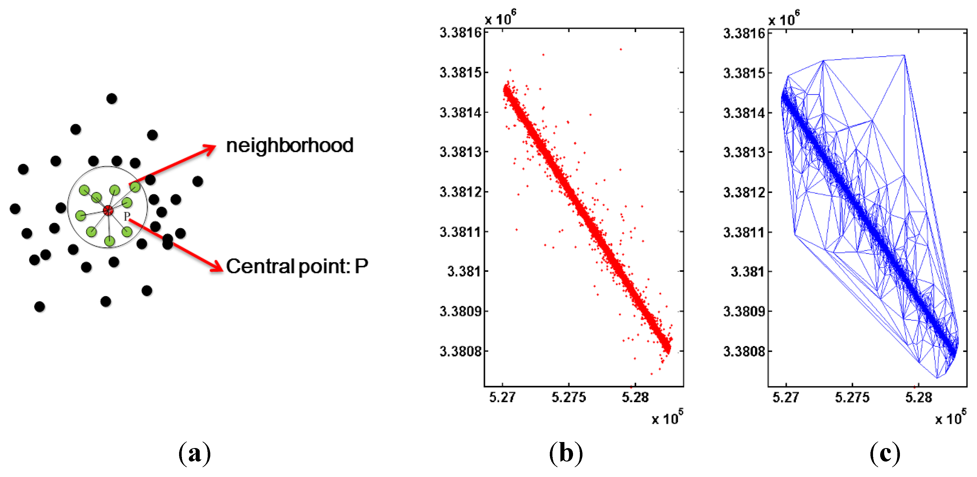
3.1.1. Adaptive Density Optimization Method

A tracking point P is defined as high-density point if the points in the neighborhood of tracking point P display a high clustering degree (Figure 2a).The density of points can be represented as a significance and tested to identify significant high-density point clusters. The null distribution [33,34] of any point dataset can be defined as:
P ( N ( A ) = k ) = λ k ( | A | k ) k ! e λ | A |
where N(A) is the number of points in any subset denoted by A (e.g., Figure 2b), k = 1,2, …, N(A), |A| is the area of subset A, λ is the intensity of the null distribution, and can be estimated as:
λ = N ( A ) | A |
Therefore, the significance of the aggregation of points in neighborhood can be calculated as:
P ( X n i ) = 1 m = 0 n i 1 ( | N e i | m ) e λ | N e i | λ m m !
where x denotes any point in the subset A, P(xni) is the significance of x, ni is the number of the points in the neighborhood of x, |Nei| is the area of neighborhood of x, r is the radius of neighborhood of x.
| N e i | = π r 2
In order to simplify the calculation, the radius r is used to indicate |Nei|. Thus Equation (3) can be simplified as:
P ( X n i ) = 1 m = 0 n i 1 ( | r | m ) e λ | r | λ m m !
For different point datasets, the radius r is adaptive, depending on the spatial distribution of points. Thus, based on a Delaunay triangulation, the radius of neighborhood is statistically defined as:
r = meanDE + variationDE
where meanDE is the mean length of all edges of the Delaunay triangulation, and variationDE is the standard deviation of the length of all edges in the Delaunay triangulation (see Figure 2c). The area of A is computed as:
| A | = i = 1 M A T i
where M is the number of triangles in the Delaunay triangulation (see Figure 2c), ATi is the area of triangle i. Each tracking point density is computed using formulas 1–7. Then the proposed method compares the density to significance η (usually set η = 0.05 or η = 0.01), and x is defined as an actual tracking point if its significance is less than η; otherwise the point x is defined as an outlier and removed from the dataset.

3.1.2. Optimization

In order to avoid significant large vibrations on the spread of trajectories due to the changes of traffic features, such as the uncertainty of traffic flow and adding of lanes at different positions on the same road, we define a trajectory segment section (TSS) as the basic unit for trajectory optimization and lane information extraction. Each TSS is obtained by dividing the trajectory segment (TS) with a fixed length, h, as shown in Figure 3. The fixed length h for dividing TS depends largely on road construction rules of a city. For example, adding a lane on a road generally occurs when the road is within 50 m of an intersection; elsewhere, the length of a lane added on a road as a parking area for buses or taxis often is greater than 10 m. Therefore, the fixed length should be less than 50 m and greater than 10 m for a better result when extracting the number of lanes. The details for acquiring TS and TSS were recommended in [35].
Figure 3. TS and TSS. (a) is the description of TS and (b) is the depiction of TSS.
Ijgi 04 02660 g003
We assume that any TSi contains several TSSes denoted as (TSS1, TSS2, …, TSSn). The TSSi has the point set SubB and the region of Delaunay triangulation network. In Figure 4a, the black point is the part of TSi and the red points belong to TSSi. In Figure 4b, the red line shows the Delaunay triangulation for TSSi. The radius of neighborhood can be computed based on Equation (6) and the area of SubB is calculated based on Equation (7). In this way, we can avoid the limitations caused by using the same radius of neighborhood to optimize trajectories in different density regions. Moreover, the accuracy when extracting the number of lanes improves because the added lanes on a road can be detected through segment treatment.

3.2. Lane Number Extraction Based on Naïve Bayesian Classification

Although low-precision vehicle trajectories with low-sampling frequency have the advantage of low costs and a short gathering period, they are still limited by gathering accuracy and frequency even when optimized. Those limitations mean that the final lane-level clustering results might differ from the actual structure of lanes. Therefore, based on the trace feature of road plane (x(1)) and trace feature of road profile (x(2)), a priori knowledge of training samples was introduced as a constraint into the lane number extraction, and the naïve Bayesian classification of lane number extraction was proposed. The implementations are introduced in detail in an upcoming section.
Figure 4. Trajectories optimization way. (a) is the tracking points of TSi; (b) shows the Delaunay triangulation network of TSSi.
Ijgi 04 02660 g004

3.2.1. The Basic Method

For training samples T = {TSS1(x1, y1), TSS2(x2, y2), …, TSSN(xN,yN)}, sample TSSi associated with trace feature set xi and category label set yi, xi = (xi(1), xi(2)) and yi=(c1, c2, …, cK), where xi(1) and xi(2) are trace features of road plane and road profile, ci is number of lanes in a road. For instance xi(j), xi(j) ϵ xi, has several possible values such as xi(j) ϵ {aj1, aj2, …, ajl, …, ajsj}, ajl is the possible value for xi(j). Then the prior probability P(Y = ck) and conditional probability P(x(j) = ajl|Y = ck) can be calculated as:
P ( Y = c k ) = i = 1 N I ( y i = c k ) N
P ( X ( j ) = a j l | Y = c k ) = i = 1 N I ( x i ( j ) = a j l , y i = c k ) i = 1 N ( y i = c k )
where I is the indicated function, Iy(c) = 1 if c ϵ y and 0 otherwise, i = 1,2, …, N, j = 1, 2, l = 1, 2, …, sj, k = 1, 2, …, K.
Given test instance x = (x(1), x(2))T, x(1) and x(2) are the trace feature of test instance x, the posterior probability is defined as:
P ( Y = c k | X = x ) = P ( Y = c k ) j P ( X ( j ) = x ( j ) | Y = c k ) k P ( Y = c k ) j P ( X ( j ) | Y = c k )
Based on the above notations and Bayesian rule, the lane number of test instance x is determined as:
y = arg  max c k P ( Y = c k ) j = 1 2 P ( X ( j ) = x ( j ) | Y = c k )
where y is the number of lanes in test instance x, and y ϵ (c1, c2, …, cK).

3.2.2. Naïve Bayesian Classifier
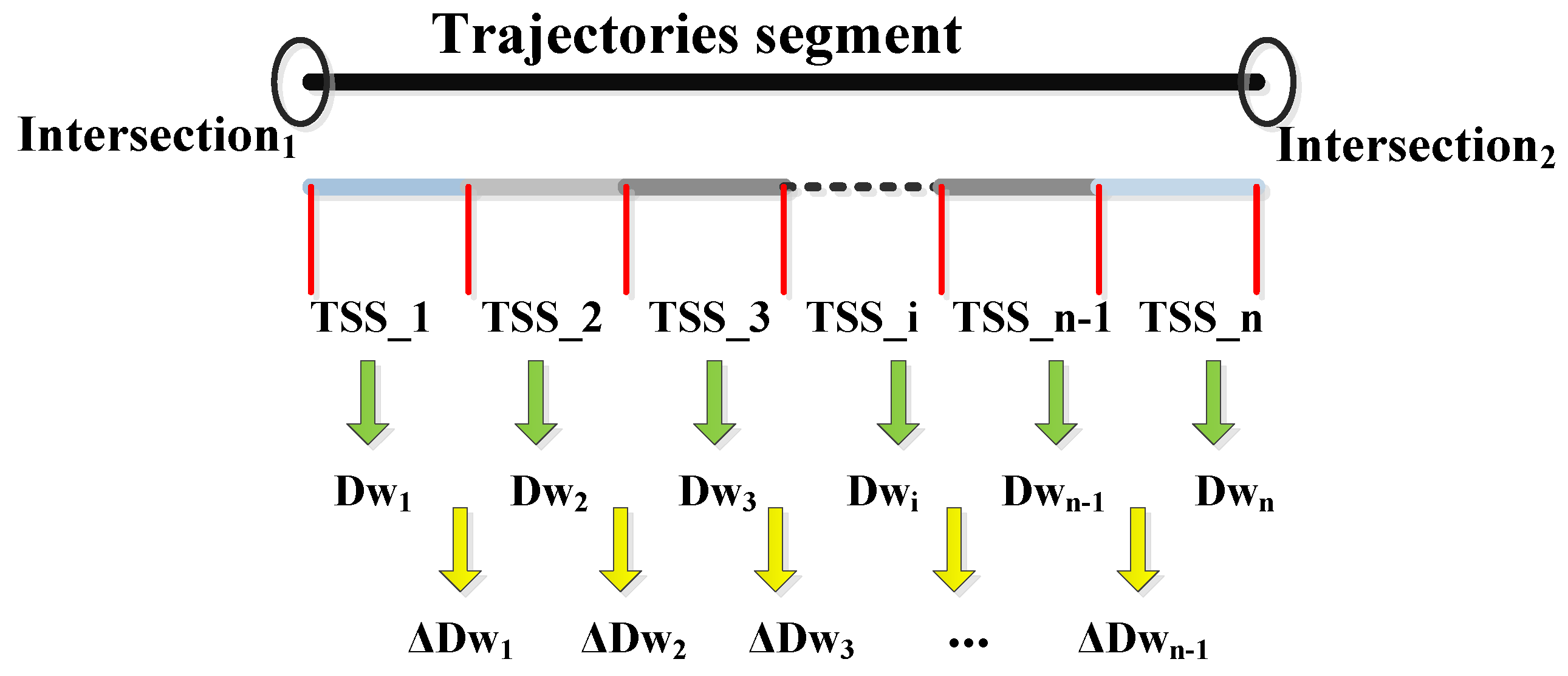
The naïve Bayesian classification determines the number of lanes in a TSS, and a naïve Bayesian classifier is thus available. The key to constructing a naïve Bayesian classifier is to acquire trace feature set xi and category set yi from the training samples T. In this study, the naïve Bayesian classifier acts as a priori knowledge for the number of lane extraction from test samples. The categorization of roads by number of lanes in the training samples must include all lane types in a city.
Trace feature set xi of training samples includes two aspects: trace feature of road plane (x(1)) and trace feature of road profile (x(2)). Millions of vehicles travel around each road in the city and gather a massive amount of tracking points that include information such as location, speed, direction and vehicle ID. A large number of tracking points cover a whole road and their coverage width will gradually become stable with an increasing number of trajectories. Road width also closely relates to the number of lanes. Thus, a trace feature of a road plane (x(1)) is the trajectories strip width (TSW) and indicates the real width of road with certain accuracy after outlier removal. Additionally, trajectories distributed on the same lane always cluster together. Thus, a trace feature of road profile (x(2)) is a cluster of a number of trajectories along the road cross-section and indicates the number of lanes to some extent.
(1) Trace Feature of Road Plane Extraction
In this paper, we propose the adaptive width detection method to detect the TSW (Figure 5).
Figure 5. The detection of trajectories strip width.
Ijgi 04 02660 g005
As shown in Figure 5, the total length of the trajectory segment TSi that starts at an intersection and ends at another intersection is L. If the fixed length is set as h, we can successively get m (m = L/h) sections as the trajectory segment section (TSS), and the diverging points of each TSS are recorded as {n1, n2, ..., nm}. The direction of the trajectory segment TSi and the diverging points are respectively set as the horizontal axis and origins of the width detection coordinate system. UYj and DYj are the positive and negative directions of the longitudinal axis, respectively. The details of the algorithm are as follows:
/*Initialization*/
Coordinate origin: n1;
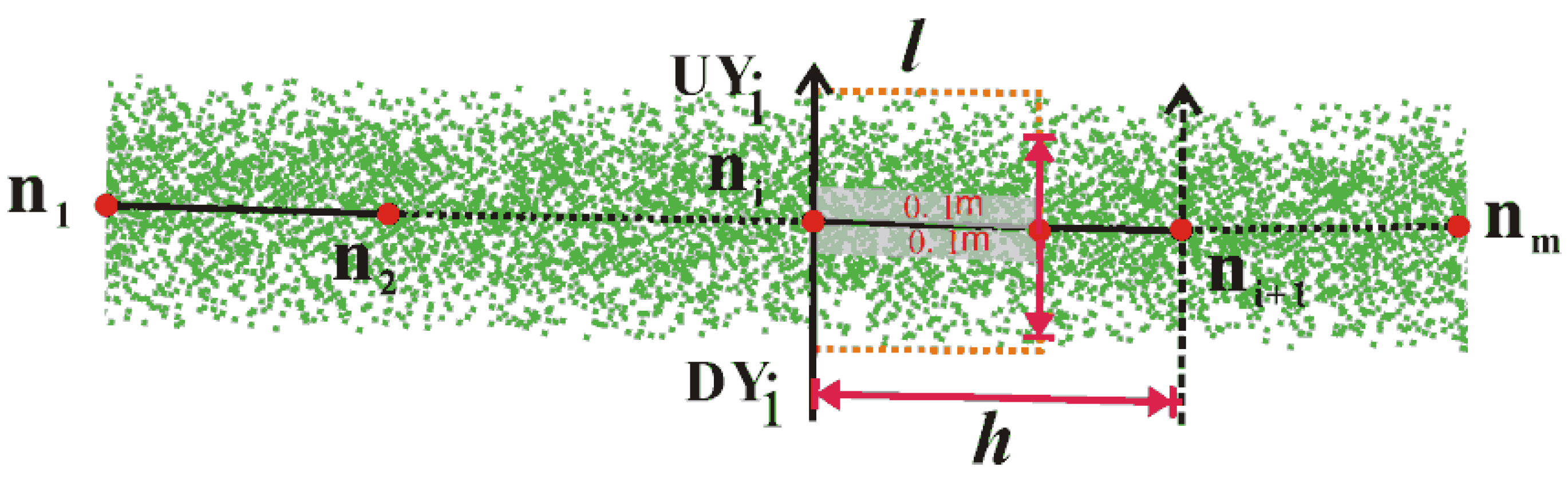
horizontal axis: the direction of the current TSS;
longitudinal axis: UYi = 0; DYi = 0;
Sliding window: length = l; width = w; proportion = 0;
/*Assignment*/
  for each TSSi, do
  repeat
    Moving the sliding window along the positive direction and negative direction of the longitudinal axis and accumulating the Proportion (Proportion = current points number in sliding window/all points in the current TSS)
   until proportion = 100%
    set Dwi = ∑ (maximum |UYj| + | maximum |DYj|)/(h/l); j = 1,2,…, (h/l).
    set Coordinate origin changed to ni+1; UYi+1 = 0;DYi+1 = 0; i = 1,2,…,m.
end for
The results for the TSS width (Dw1, Dw2, …, Dwm) are obtained as shown in Figure 6, where ΔDw1, …, ΔDwn-1 are the differences of each TSS width.
Figure 6. Trajectories strip width analysis.
Ijgi 04 02660 g006
In most cases, the value ΔDwi between two adjacent TSSes will stay within one lane width a due to position accuracy of GPS data or from added lanes. However, some abnormal results still exist due to the effects of temporary parking areas, bus stops, dense lanes appearing near intersections, etc., which make ΔDwi abnormally larger than a. Thus, the nearest measurement result of TSS replaces abnormal results considering that the width along the road is always in a relatively steady state. We will explain this approach in more detail.
Step 1, compute the difference of each TSS width between Dwi and Dwi+1, that is, ΔDwi = DwiDwi+1 (i = 1, 2, …, n − 1);
Step 2, compare each ΔDwi with a, Dwi is replaced by Dwi+1 when ΔDwi is larger than a and Dwi is larger than Dwi+1 (i = 1, 2, …, n − 1);
Step 3, do step1 and step 2 repeatedly until all abnormal values are optimized.
The results for TSS width difference are shown in Figure 7, the blue line indicates the raw results from ΔDwi, the red points are the abnormal values, and the green line shows the result of optimized ΔDwi.
Figure 7. Width detection results proprecessing.
Ijgi 04 02660 g007
(2) Trace Features of Road Profile Extraction
According to methods described previously, in the naïve Bayesian classifier, the trace feature of road profile (x(2)) is the number of clustered trajectories. The authors of [7,29,30,31] proposed using cluster methods to detect lane structure from high-precision GPS trajectories with high sampling frequency such as partition clustering, hierarchical clustering and statistical clustering. According to reference [7] statistical clustering is more suitable for lane structure detection from ordinary GPS data at an accuracy within 4 m. Therefore, for acquiring cluster number of trajectories in road profiles, we fit a constrained Gaussian mixture model (CGMM) to perpendicular cross-sections of the traces across the road, based on the assumption that GPS trajectories will tend to cluster near the center of each lane with some spread due to GPS noise and other vagaries. The CGMM can be defined as:
p ( x ) = ( j = 1 ln ω j 1 2 π σ 2 exp ( ( x μ j ) 2 2 σ 2 ) )
where ln represents the number of Gaussian components, and each component corresponds to each lane, while w1, …, wln are the weights of each component, corresponding to the relative traffic volume in each lane and j = 1 l n w j = 1 . The μ1, …, μln is the means of the trajectories for each component and equals to the centerline of each lane; σ is the standard variance of the trajectories for each component and set same value because the width of lane of adjacency lane usually is the same. The number of components for a CGMM is equal to cluster number of trajectories of a TSS and determined by the structural risk model (structural risk minimization, SRM). To estimate wi, ui and σ for a set of ln’s and then select the ln that minimizes the structural risk model. The method to calculate and extract the number of clusters can be obtained according to [7].
In addition, a trajectory is a line described by a series of points. Each point has a gathering time and spatial location, such as Tracei = {p1, p2, …, pn}, pi = (xi, yi, ti, directioni, speedi, statei) (i = 1, 2, …, n), where (xi, yi) is the spatial location, ti is the gathering time, and directioni and speedi give the motion status of a moving object. At the same time, statei is attributed information of a moving object such as the ID number of a moving object, as shown in Figure 8a. However, this description is not appropriate for analyzing the longitudinal density distribution of low-quality trajectories because the sampling intervals of this kind of data range from ten seconds to one minute, making the distance between any two adjacent points too large to retain enough information. Thus, we replace common trajectories with trajectory vectors, and obtain a number of trajectories clusters by detecting the longitudinal density distribution of those trajectory vectors.
For each trajectory vector, the tracking point is regarded as the start point, the direction of tracking point as vector direction, and the speed as the vector mold. The tracking point is denoted as Pi (xi, yi, ti, directioni, speedi, statei), and its trajectory vector is described as Travectori = (xi, yi) and |Travectori| = speedi × Δt, Δt = 1 s (Δt does not affect the final outcome for GMM computation, this paper set it as 1 s), as shown in Figure 8b.
To facilitate CGMM computation, we rotate the axes so that the X axis is made parallel to the average direction vector. Here, the rotation matrix in Equation (13) is used. The angle ξ can be obtained according to [35].
[ x ' y ' ] = [ cos ξ sin ξ sin ξ cos ξ ] [ x y ]
The longitudinal density distribution of trajectories is acquired by projecting each trajectory vector to the vertical axis (y'). The projecting ordinate of each trace vector is set as the sampling point and replaces the intersection points of trajectories and sampling lines perpendicular to the road centerline.
Figure 8. Trajectories and trajectory vector description. (a) shows the trajectory vector constructed according to traditional style; (b) is the trajectory vector proposed in this paper.
Ijgi 04 02660 g008

3.3. The Detection of Turn Rules of Each Lane

GPS trajectories are a sequence of GPS points with the time interval between any consecutive GPS points not exceeding a certain threshold ΔT (ΔT is the sampling interval.), as shown in Figure 9. We detect the turn rules of each lane by tracking GPS trajectories. Figure 9 illustrates the trajectories of vehicles. Figure 9a shows trajectories at a 40 s sampling interval. Figure 9b indicates the trajectories at a 20 s sampling interval. Figure 9c shows different driving directions of vehicles and the sample rate of trajectories is 20 s, where the red lines represent the turn rules of each vehicle from north to south, the green lines denote the south to north direction, the blue and yellow lines indicate vehicle right turns.
Figure 9. Trajectory tracking. (a) indicates the trajectories with 40 s sampling interval; (b) shows the trajectories with 20 s sampling interval; (c) descripts the different driving directions of vehicles.
Ijgi 04 02660 g009
Through recording the trajectory segments, the change of trajectory direction is replaced by the change of the trajectory segments’ direction. Figure 10 indicates the trajectory belonging to segments TS001 and TS004. The change of direction between TS001 and TS004 is computed as Δθ = θ2 − θ1; these (θ1, θ2) are directions of TS001, TS004 obtained by [34]. The turn rules of the lane traversed by the trajectory are “left Turn,” “right turn,” “going straight” and “U-turn,” if change of direction satisfies the conditions: (Δθ < 0° & Δθ ≈ −90°), (Δθ > 0° & Δθ ≈ 90°), (Δθ ≈ 0°) and (Δθ > 0° & Δθ ≈ 180°), respectively. The turn rules of each lane are further determined by Equation (14).
f i = v a l u e i i = 1 4 v a l u e i ( i = 1 , 2 , 3 , 4 )
That valuei is the number of GPS trajectories belonging to groupi (i = 1, 2, 3, 4 indicates “left turn,” “right-turn,” “going straight” and “U-turn,” respectively) on the lane. The final rate of groupi on the lane is denoted as fi. The turning of the lane is groupi if fi is far beyond a predefined rate of reckless driving.
Figure 10. Intersection turns: left turn, right turn and U-turn detection.
Ijgi 04 02660 g010

4. Experiments and Results

Our test GPS data came from thousands of taxis driving in Wuhan city, as shown in Figure 11a. The sampling frequency ranges from 10 s to 40 s, while the positioning accuracy ranges from 10 m to 15 m. Each taxi was recorded for an average of 14 days, and we collected in total about 200 billion GPS points, as shown in Figure 11b. We obtained about 2000 TS, and 300,000 TSS when the fixed length h was set as 10 m. The number of trajectory vectors in each TSS ranges from 100 to 1000.
Figure 11. Experimental data. (a) is the road network of the experimental area; (b) shows the raw trajectories collected by taxis.
Ijgi 04 02660 g011

4.1. Trajectory Optimization

Outliers mixed in raw GPS trajectories were eliminated using the adaptive density optimization method. The trajectory strip width (TSW) of each TSS was obtained and optimized using our proposed adaptive width detection method. The length l and width w of the sliding window were set as 10 m and 0.1 m, respectively; the significance η was set as 0.05, as recommended by reference [33]; and the width of lane a for optimized trajectories was set as 3.75 m according to the road construction standards in China. Figure 12 shows the results of trajectory optimization, where red points and black points represent the valid data and outliers, respectively.
Figure 12. Optimization results. The result of all experimental data (left); the magnification of one segment (right).
Ijgi 04 02660 g012
Figure 13. Optimization results evaluation: (a) shows the evaluation results of optimized trajectories; (b) indicates the evaluation results of non-optimized trajectories.
Ijgi 04 02660 g013
An evaluation for trajectory optimization results was done by comparing with the correlation between TSW before and after optimization and the actual road width, as shown in Figure 13. The test data (about 400 TSS) were randomly selected from the 300,000 TSS, the trajectory strip width (TSW) before and after optimization was acquired using adaptive width detection algorithm, and the actual width of the road was obtained by field measurement. Based on statistics, the strong correlation (R2 = 0.9633) between TSW and actual width of road of each optimized TSS illustrates that TSW of optimized TSS is very close to the actual road width. Comparing with the non-optimization results (Figure 13b), the optimization results indicate that the proposed optimization method performs well.

4.2. The Construction of Naïve Bayesian Classifier

A selection of TSSes (about 7,650 TSSes) found on various types of lanes in the experimental area were used as training samples, and the other 11,350 TSSes were designated as test samples. The real number of lanes in the training sample was extracted by observing a corresponding remote sensing image. By analyzing the relation between the real number of lanes, the trajectory strip width (TSW) and number of clusters in the training sample, we established a naïve Bayesian classifier, as listed in Table 1.
Table 1 indicates the categories of the number of lanes in the experimental area including two-lane, three-lane, four-lane and five-lane roads. Each type contains three values, such as the value of TSW (x(1)), the number of trajectories clusters (x(2)) and the real number of lanes (y) for the training sample.

4.3. Lane Information Extraction

Given a test instance TSS (13.8m, 3)T, the lane number is calculated as:
P(y = 2) = 278/765; P(y = 3) = 220/765; P(y = 4) = 189/765; P(y = 5) = 78/765;
P(x(1) = 13.8 | y = 2)=0/278; P(x(2) = 3|y = 2) = 98/278;
P(x(1) = 13.8 | y = 3) = 220/220; P(x(2) = 3 | y = 3) = 185/220;
P(x(1) = 13.8 | y = 4) = 189/189; P(x(2) = 3 | y = 4) = 34/189;
P(x(1) = 13.8 | y = 5) = 0/78; P(x(2) = 3|y = 5)=5/78;
P(y = 2) * P(x(1) = 13.8 | y = 2) * P(x(2) = 3 | y = 2) = 0;
P(y = 3) * P(x(1) = 13.8 | y = 3) * P(x(2) = 3 | y = 3) = 0.242;
P(y = 4) * P(x(1) = 13.8 | y = 4) * P(x(2) = 3 | y = 4) = 0.044;
P(y = 5) * P(x(1) = 13.8|y = 5) * P(x(2) = 3|y = 5) = 0.
Table 1. Naïve Bayesian classifier.
Training Sample (ID)Trace Feature: x(1)/mTrace Feature: x(2)Category Label Set: y
17.9–12.222
27.9–12.232
2,7807.9–12.222
2,78110.2–19.833
2,78210.2–19.833
4,98010.2–19.843
4,98113.2–20.844
4,98213.2–20.844
6,87013.2–20.834
6,87117.6–25.845
6,87217.6–25.855
7,65017.6–25.855
Table 2. Lane information identification.
TSTSSx(1)/mx(2)The Number of Lanes (Detections)The Number of Lanes (True Value)Driving Direction (Detections)Driving Direction (True Value)
TS001TSS00110.1222 Ijgi 04 02660 i001 Ijgi 04 02660 i001 Ijgi 04 02660 i001 Ijgi 04 02660 i001
TSS0029.9222 Ijgi 04 02660 i001 Ijgi 04 02660 i001 Ijgi 04 02660 i001 Ijgi 04 02660 i001
TS002TSS00114.1443 Ijgi 04 02660 i001 Ijgi 04 02660 i001 Ijgi 04 02660 i001 Ijgi 04 02660 i002 Ijgi 04 02660 i001 Ijgi 04 02660 i001 Ijgi 04 02660 i002
TSS00214.2443 Ijgi 04 02660 i001 Ijgi 04 02660 i001 Ijgi 04 02660 i002 Ijgi 04 02660 i001 Ijgi 04 02660 i001 Ijgi 04 02660 i002
TSS01615.4333 Ijgi 04 02660 i001 Ijgi 04 02660 i001 Ijgi 04 02660 i002 Ijgi 04 02660 i001 Ijgi 04 02660 i001 Ijgi 04 02660 i002
TS003TSS00119.2444 Ijgi 04 02660 i001 Ijgi 04 02660 i001 Ijgi 04 02660 i001 Ijgi 04 02660 i002 Ijgi 04 02660 i001 Ijgi 04 02660 i001 Ijgi 04 02660 i001 Ijgi 04 02660 i002
TSS00220.3444 Ijgi 04 02660 i001 Ijgi 04 02660 i001 Ijgi 04 02660 i001 Ijgi 04 02660 i002 Ijgi 04 02660 i001 Ijgi 04 02660 i001 Ijgi 04 02660 i001 Ijgi 04 02660 i002
TSS00320.3334 Ijgi 04 02660 i001 Ijgi 04 02660 i001 Ijgi 04 02660 i001 Ijgi 04 02660 i002 Ijgi 04 02660 i001 Ijgi 04 02660 i001 Ijgi 04 02660 i001 Ijgi 04 02660 i002
TSS04220.3553 Ijgi 04 02660 i001 Ijgi 04 02660 i001 Ijgi 04 02660 i001 Ijgi 04 02660 i002 Ijgi 04 02660 i002 Ijgi 04 02660 i001 Ijgi 04 02660 i001 Ijgi 04 02660 i002
Thus, according to Equation (11), the number of TSS lanes were 3. Specifically, the road centerline of TSS was acquired according to [26], then we inferred the lane boundary based on the number of lanes of TSS with the width of lane a. Turn rules of each lane is determined according to Equation 14. At the same time, according to the road construction standard in China, the lane width a is set to 3.75 m, and the predefined rate of reckless driving for turn information extraction is set as 5%. Table 2 indicates the other results of lane information detection for each TSS, including number of lanes and driving directions of each lane.
In Table 2, most results show the stability and the validity of lane information extraction using a naïve Bayesian classifier, but a few mistakes still occurred. For example, numbers of lanes such as TSS001 of TS002, and TSS042 of TS003 were misclassified. We use arrow-shaped indications to represent the driving directions of each lane, where arrow-shaped indication Ijgi 04 02660 i001 
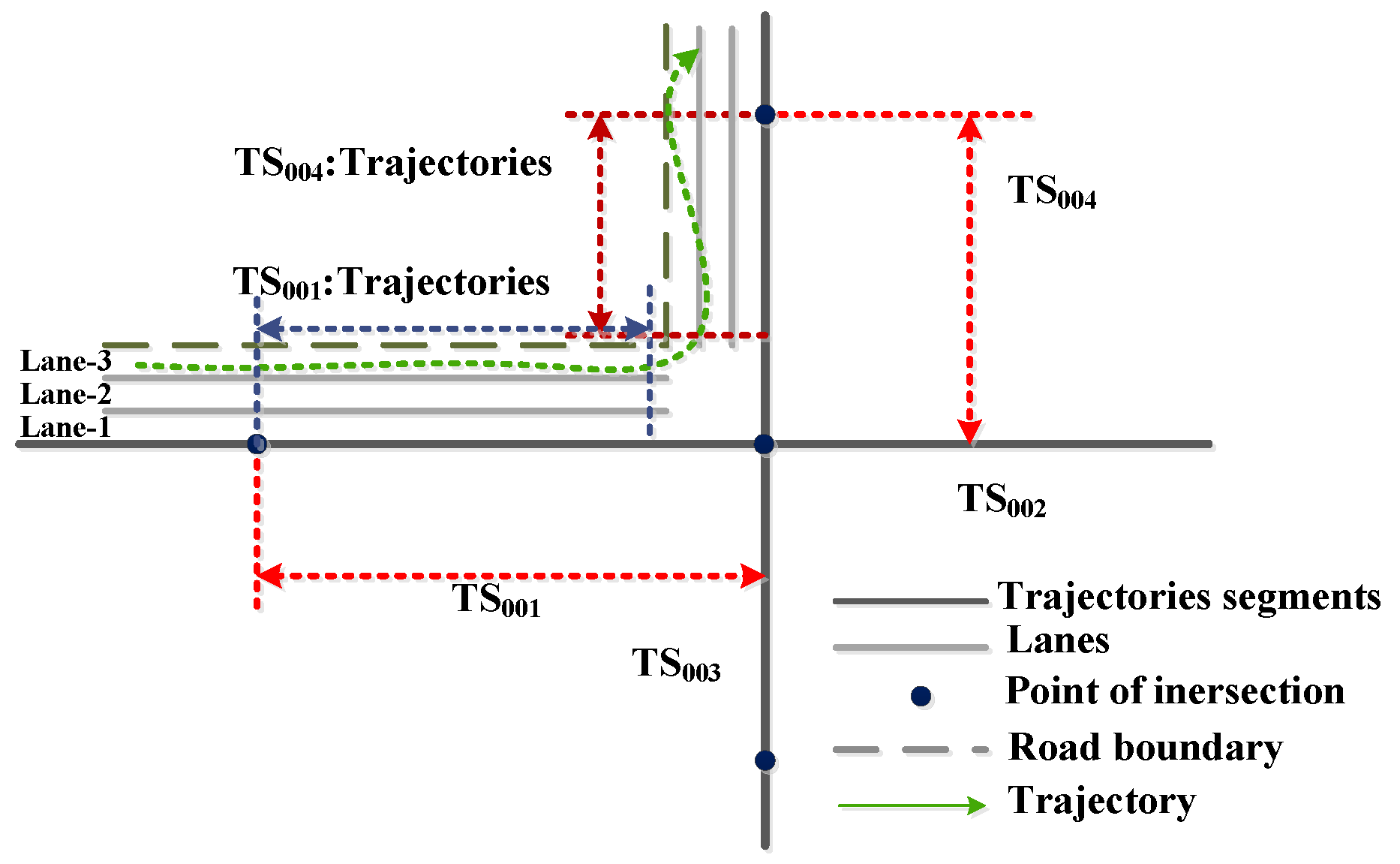
indicates that vehicle drivers go straight, and multi-headed arrows Ijgi 04 02660 i002 show that vehicle drivers can travel in straight direction or turn left at an intersection, as shown in Table 2. At the same time, the accuracy of turn rules of lane detection depends largely on the results of the number of lanes. In Table 2, the turn rules from lanes in the test samples also get a misclassification because of an incorrect estimate of the number of lanes.

4.4. Quantitative Evaluation

4.4.1. Quantitative Evaluation for Number of Lane Identification

To evaluate the performance of our proposed method for detecting lane information, we compared test samples for the number of lanes extraction to those manually marked. Table 3 shows quantitative values for precision, recall, and f-score in the proposed method (MLIT) and the methods of [29,30,31]. This comparison demonstrates that MILT has better precision, recall, and f-score in lane number extraction than those of [29,30,31]. Meanwhile, the result of this comparison shows that MLIT is more suitable for low-precision GPS trajectories with low-sampling frequency than other methods of [29,30,31] that detects lane structure directly from raw trajectories, but does not consider the prior knowledge during lane number identification. At the same time, experimental results also authenticate that low-precision GPS trajectories from different lanes are not separated well. In addition, Table 3 shows that the proposed method extracts the lane numbers with an overall accuracy of 83.72%; however, there is also a 16.68% chance of incorrectly identifying the number of lanes. The reasons are as follows.
First, MLIT has a difficulty in lane number identification because a small number of complex intersections (e.g., the incorrect results in Table 2) have different traffic flows between adjacent lanes caused by traffic lights, driving restrictions, and other traffic characteristics.
Second, MLIT cannot distinguish trajectories from roads on and below viaducts, since the experimental data has no elevation information. The lane information for overlapping roads in the study area was misclassified.
Lastly, the number of lanes can be missed because of GPS signal loss in tunnels.
Such misclassifications require further investigation to improve the accuracy classification of road segments by number of lanes. In summary, our method performs much better than other methods for number of lanes identification from low-precision GPS trajectories with low-sampling frequency.
Table 3. Quantitative evaluation and comparison.
MethodsPrecisionRecallF-Score
MLIT83.72%83.35%84.03%
Kernel density estimation [31]78.48%79.05%78.76%
Hierarchical agglomerative clustering [30]63.23%62.7%62.96%
K-means clustering [29]62.54%61.51%62.02%

4.4.2. Quantitative Evaluation for Turn Rules Detection

To evaluate the performance of the proposed method for turn rules of each lane, we compared turn information of two intersections calculated by MLIT with that of manually marked roads. In Figure 14, intersections were randomly selected from a database and the trajectories that traversed those intersections were used to detect turn rules of each lane. The results show that the overall accuracy for turn information classification was 81.3% when comparing our detection results with the actual turn rules, assuming the rate of non-standard driving was 5%. The accuracy of turn rules of each lane identification is lower than the number of lane extraction because it depends not just on the accuracy of lane number identification, but driver behavior and data precision as well.
Figure 14. The overlay of image and trajectories. (a) shows the tracking results of one intersection; (b) indicates the tracking results of another intersection.
Ijgi 04 02660 g014

5. Conclusions

In this paper, we proposed an automated method (MLIT) to extract lane information, such as numbers of lane and lane turns on road segments from low-precision GPS trajectory data. On one hand, the proposed method (MLIT) eliminates outliers from GPS trajectory data using adaptive density optimization, method improving the robustness of the lane information detection. On the other hand, MILT detects the exact numbers of lanes in TSSes by combining prior knowledge with trace features of road planes and road profiles, resulting in robust extraction of numbers of lanes. However, MLIT still has room for improvement, and the future work will continue to focus on trajectory optimization and extraction of lane information in complex road environments such as tunnels, or overpasses.

Acknowledgments

The research presented here was funded by the National Natural Science Foundation of China (No. 41571430, 41271442, 40801155), and the open research fund of the Academy of Satellite application (2014_CXJJ-DSJ_02). We acknowledge Shenzhen Science Technology Bureau for institutional support.

Author Contributions

Luliang Tang and Xue Yang conceived and designed the algorithms of MLIT presented in this paper. Xue Yang performed the experiments and wrote the paper. Zihan Kan and Qingquan Li contributed analysis tools.

Conflicts of Interest

The authors declare no conflict of interest.

References

  1. Gonzalez, J.P.; Ozguner, U. Lane detection using histogram-based segmentation and decision trees. In Proceedings of 2000 IEEE Intelligent Transportation Systems, Dearborn, MI, USA, 1–3 October 2000.
  2. Wang, Y.; Teoh, E.K.; Shen, D. Lane detection using B-snake. In Proceedings of 1999 International Conference on Information Intelligence and Systems, Bethesda, MD, USA, 3 October 1999.
  3. Hillel, A.B.; Lerner, R.; Levi, D.; Raz, G. Recent progress in road and lane detection: A survey. Mach. Vis. Appl. 2014, 25, 727–745. [Google Scholar] [CrossRef]
  4. Kammel, S.; Pitzer, B. Lidar-based lane marker detection and mapping. In Proceedings of Intelligent Vehicles Symposium, Eindhoven, the Netherlands, 4–6 June 2008.
  5. Thuy, M.; León, F. Lane detection and tracking based on Lidar data. Metrol. Meas. Syst. 2010, 17, 311–321. [Google Scholar] [CrossRef]
  6. Yang, B.S.; Dong, Z.; Zhao, G.; Dai, W.X. Hierarchical extraction of urban objects from mobile laser scanning data. ISPRS J. Phothogr. Remote Sens. 2015, 99, 45–57. [Google Scholar] [CrossRef]
  7. Chen, Y.H.; Krumm, J. Probabilistic modeling of traffic lanes from GPS traces. In Proceedings of the 18th SIGSPATIAL International Conference on Advances in Geographic Information Systems, San Jose, CA, USA, 2–5 November 2010.
  8. Yeh, A.G.O.; Zhong, T.; Yue, Y. Hierarchical polygonization for generating and updating lane-based road network information for navigation from road markings. Int. J. Geogr. Inf. Sci. 2015, 29, 1509–1533. [Google Scholar] [CrossRef]
  9. Liu, X.T.; Ban, Y.F. Uncovering spatio-temporal cluster patterns using massive floating car data. ISPRS Int. J. Geo-Inf. 2013, 2, 371–384. [Google Scholar] [CrossRef]
  10. Sainio, J.; Westerholm, J.; Oksanen, J. Generating heat maps of popular routes online from massive mobile sports tracking application data in milliseconds while respecting privacy. ISPRS Int. J. Geo-Inf. 2015, 4, 1813–1826. [Google Scholar] [CrossRef]
  11. Zheng, Y.; Zhang, L.; Xie, X.; Ma, W.Y. Mining interesting locations and travel sequences from GPS trajectories. In Proceedings of 18th International World Wide Web Conference, Madrid, Spain, 20–24 April 2009.
  12. Giannotti, F.; Nanni, M.; Pinelli, F.; Pedreschi, D. Trajectory pattern mining. In Proceedings of 13th ACM SIGKDD International Conference on Knowledge Discovery and Data Mining, San Jose, CA, USA, 12–15 August 2007.
  13. Yin, P.; Ye, M.; Lee, W.C.; Li, Z. Mining GPS data for trajectory recommendation. In Advances in Knowledge Discovery and Data Mining; Springer: Cham, Switzerland, 2014; pp. 50–61. [Google Scholar]
  14. Tang, L.L; Chang, X.M.; Li, Q.Q. Public travel route optimization based on ant colony optimization algorithm and taxi GPS data. China J. Highw. Transp. 2011, 24, 89–95. [Google Scholar]
  15. Wang, J.; Rui, X.; Song, X.; Tan, X. A novel approach for generating routable road maps from vehicle GPS trajectories. Int. J. Geogr. Inf. Sci. 2014, 29, 69–91. [Google Scholar] [CrossRef]
  16. Tang, L.L.; Huang, F.Z.H.; Zhang, X.Y.; Li, Q.Q. Road Network change detection based on floating car data. J. Netw. 2012, 7, 1063–1070. [Google Scholar] [CrossRef]
  17. Zhou, B.D.; Li, Q.Q.; Mao, Q.Z.H.; Tu, W.; Zhang, X.; Chen, L. ALIMC: Activity landmark-based indoor mapping via crowdsourcing. IEEE Trans. Intell. Transp. Syst. 2015, 16, 2774–2785. [Google Scholar] [CrossRef]
  18. De Fabritiis, C.; Ragona, R.; Valenti, G. Traffic estimation and prediction based on real time floating car data. In Proceedings of 11th International IEEE Conference on Intelligent Transportation Systems (ITSC), Beijing, China, 12–15 October 2008.
  19. Sun, D.; Zhang, C.; Zhang, L.; Chen, F.; Peng, Z.R. Urban travel behavior analyses and route prediction based on floating car data. Trans. Lett. Int. J. Trans. Res. 2014, 6, 118–125. [Google Scholar] [CrossRef]
  20. Lee, W.C.; Krumm, J. Trajectory preprocessing. In Computing with Spatial Trajectories; Zheng, Y., Zhou, X., Eds.; Springer: New York, NY, USA, 2011; pp. 3–33. [Google Scholar]
  21. Brakatsoulas, S.; Pfoser, D.; Salas, R.; Wenk, C. On map-matching vehicle tracking data. In Proceedings of 31st International Conference on Very Large Data Bases, Trondheim, Norway, 30 August–2 September 2005.
  22. Haklay, M.; Weber, P. OpenStreetMap: User-generated street maps. IEEE Perv. Comput. 2008, 7, 12–18. [Google Scholar] [CrossRef]
  23. Yanagisawa, Y.; Akahani, J.; Satoh, T. Shape-based similarity query for trajectory of mobile objects. In Proceedings of 4th International Conference on Mobile Data Management, Melbourne, Australia, 21–24 January 2003.
  24. Bruntrup, R.; Edelkamp, S.; Jabbar, S. Incremental map generation with GPS traces. In Proceedings of the 2005 IEEE Intelligent Transportation Systems, Vienna, Austria, 13–15 September 2005.
  25. Li, J.; Qin, Q.; Xie, C.; Zhao, Y.; Li, J.; Qin, Q. Integrated use of spatial and semantic relationships for extracting road networks from floating car data. Int. J. Appl. Earth Obs. Geoinf. 2012, 19, 238–247. [Google Scholar] [CrossRef]
  26. Liu, C.H.Y.; Xiong, L.; Hu, X.Y.; Shan, J. A progressive buffering method for road map update using OpenStreetMap data. ISPRS Int. J. Geo-Inf. 2015, 4, 1246–1264. [Google Scholar] [CrossRef]
  27. Li, Q.Q.; Tang, L.L.; Zuo, X.Q.; Li, H.W. Transect-based three dimensional road modeling and visualization. Geo-Spat. Inf. Sci. 2004, 7, 14–17. [Google Scholar]
  28. Pollak, K.; Peled, A.; Hakkert, S. Geo-based statistical models for vulnerability prediction of highway network segments. ISPRS Int. J. Geo-Inf. 2014, 3, 619–637. [Google Scholar] [CrossRef]
  29. Wagstaff, K.; Cardie, C.; Rogers, S.; Schroedl, S. Constrained k-means clustering with background knowledge. In Proceedings of 18th International Conference on Machine Learning (ICML), Williamstown, MA, USA, 28 June–1 July 2001.
  30. Edelkamp, S.; Schrödl, S. Route planning and map inference with global positioning trajectories. Comput. Sci. Perspect. 2003, 2598, 128–151. [Google Scholar]
  31. Uduwaragoda, A.; Perera, A.S.; Dias, S.A.D. Generating lane level road data from vehicle trajectories using kernel density estimation. In Proceedings of the 16th International IEEE Annual Conference on Intelligent Transportation Systems (ITSC), Hague, the Netherlands, 6–9 October 2013.
  32. Han, J.; Kamber, M. Mining stream, time-series, and sequence data. In Data mining: Concepts and techniques; Asma, S., Ed.; Elsevier: USA, 2011; pp. 467–531. [Google Scholar]
  33. Shekhar, S.; Evans, M.R.; Kang, J.M.; Pradeep, M. Identifying patterns in spatial information: A survey of methods. WIREs Data Min. Knowl. Discov. 2011, 1, 193–214. [Google Scholar] [CrossRef]
  34. Liu, Q.; Tang, J.; Deng, M.; Shi, Y. An iterative detection and removal method for detecting spatial clusters of different densities. Trans. in GIS 2015, 19, 82–106. [Google Scholar] [CrossRef]
  35. Lee, J.G.; Han, J. Trajectory clustering: A partition-and-group framework. In Proceedings of the 2007 ACM SIGMOD International Conference on Management of Data, Beijing, China, 11–14 June 2007.

