Accuracy and Effort of Interpolation and Sampling: Can GIS Help Lower Field Costs?

Abstract

Sedimentation is a problem for all reservoirs in the Black Hills of South Dakota. Before working on sediment removal, a survey on the extent and distribution of the sediment is needed. Two sample lakes were used to determine which of three interpolation methods gave the most accurate volume results. A secondary goal was to see if fewer samples could be taken while still providing similar results. The smaller samples would mean less field time and thus lower costs. Subsamples of 50%, 33% and 25% were taken from the total samples and evaluated for the lowest Root Mean Squared Error values. Throughout the trials, the larger sample sizes generally showed better accuracy than smaller samples. Graphing the sediment volume estimates of the full sample, 50%, 33% and 25% showed little improvement after a sample of approximately 40%–50% when comparing the asymptote of the separate samples. When we used smaller subsamples the predicted sediment volumes were normally greater than the full sample volumes. It is suggested that when planning future sediment surveys, workers plan on gathering data at approximately every 5.21 meters. These sample sizes can be cut in half and still retain relative accuracy if time savings are needed. Volume estimates may slightly suffer with these reduced samples sizes, but the field work savings can be of benefit. Results from these surveys are used in prioritization of available funds for reclamation efforts.

1. Introduction

Interpolation of data between sampled points is both powerful and timesaving. It allows for the estimation of values between the known values, yet provides a cost savings as workers do not need to collect excess data from many additional sites or repeated field excursions; however, accuracy questions regarding the interpolated values do arise after the algorithm is used [1,2,3]. Evaluations of interpolation techniques have been determined across environmental disciplines such as rainfall [4,5], wind velocity [6], air temperatures [6] and evapotranspiration studies [1] and others. However, evaluations of interpolation involving sediment data are rarely studied and never has a study such as this occurred in the Black Hills of South Dakota. The analysis of different interpolation methods, investigation of sample size, and verification of these findings with real-world scenarios provides valuable information for sediment removal in reclamation efforts.

Using sediment data is valuable as it allows for an initial investigation of sediment deposition, how it exists spatially within a reservoir and it makes available the background for repeat measures when investigating temporal changes [7]. Determining the amount of sediment in a reservoir is important in regards to the life expectancy of reservoirs and in determining if any land management practices can prolong this period. Mounting evidence for appropriate watershed planning can assist or prolong the life expectancy of any given reservoir and its tendency to fill in with sediment. Deposition of sediment within a reservoir has been predicted through modeling processes but remains stochastic in nature in regards to natural fluctuations of inflow, water level, sediment concentrations and climatic conditions [8,9,10].

The Black Hills are an elliptically domed area in southwestern South Dakota and northeastern Wyoming, with limestone prominent in regards to hydrologic importance [11]. Permanent water sources occur in fractured sections of the limestone formations as subsurface aquifers intersect the land surface as coldwater springs [12]. The Black Hills are unique in that few streams exit from the region and there were originally only small pools of water, mostly originating from beaver (Castor canadensis) activity [13]. Most streams are ephemeral, readily available ponded waters are almost nonexistent and the technology to extract water from aquifers during early settlement has not been developed. Efforts by early settlers to develop a consistent water source occurred with the construction of artificial dams to capture surface runoff and were augmented by the Civilian Conservation Corps (CCC) and U.S. Forest Service (USFS). Today, these small waters (0.8 hectare to 12.1 hectare) are nearly 80 years old and have reached a level of “maturity” by limnology standards [14,15].

Aging of these waters, including sediment influx naturally occurs over time, but can be accelerated by upstream influences such as overgrazing by livestock and road building practices [8,16,17]. Today’s users are directly impacted by the buildup of sediment and how it affects their recreation. Many of these small reservoirs are showing the effects of increased sediment, such as shallowing of the lake and subsequent cattail (Typha sp.) intrusion. Measures by the author at one local reservoir showed sediment depths of nearly three meters in depth. These sediment increases have an impact on fisheries management in several ways.

These impacts affect how anglers can access the waters and the survival of trout once they are introduced into the system. The State of South Dakota annually manages many of these small dams as put-and-take fisheries through Rainbow Trout (Oncorhynchus mykiss) stockings. Recent finding at two waters, similar to those of the waters in this study, showed an estimated recreational fishing use of over 5239 h in one summer alone [18]. Keeping these fisheries available to the angler may require maintenance, such as the removal of sediment when it interferes with fishing access. The presence of coldwater fish, such as Rainbow Trout, can also be hampered due to shallow waters and the effects of sunlight elevating temperature that may further lessen fish survival. However, removal of the sediment has been costly in past projects and many unknown factors arise in the bidding process.

Collecting field data and incorporating GIS interpolation allows for estimation of the volume of sediment in a waterbody. By providing needed data for cost estimates, public agencies and private enterprises can forecast expenditures, while saving time and money by reducing last minute contract changes. Additionally, public decision makers can also use these estimates to aid in determining how these expenditures rank in regards to other projects and appropriate areas for spoil deposits.

There are three objectives in this research. Firstly was to determine the best of three interpolation methods for representing Black Hills sediment data based on the accuracy of predicted interpolated points to actual data values. There are many different approaches towards determining estimated volume of sediment [19,20]. Spatial regression is one technique that could produce the statistic surfaces and determine an estimate for total sediment. Using spatial regression is attractive when one is looking at multiple variables in that they can be measured together at the same time, ranked by importance and effects evaluated. In this study, we were not investigating different variables and possible interactions involving sediment deposition. Different algorithms used to derive spatial interpolation will produce unique surfaces from the same set of point data. Even changing parameters within a specific algorithm will generate a different surface. Currently, there is no accepted practice to determine which algorithms will generate the most accurate surfaces under a given set of circumstances. Therefore, it is important to evaluate surfaces for accuracy. Secondly, to investigate the differences in sample size in an effort to determine if reduced efforts would produce satisfactory results to larger sample sizes. This last effort was initiated to decide if lowered fieldwork would produce acceptable results and allow for reduced project costs by further evaluating the effects of sample size in a graphing procedure to determine improvements of estimates with increased samples.

2. Materials and Methods

Sediment and water depth measurements were gathered during the winter when ice conditions were safe for workers. Data were gathered in a grid like fashion taking into account points, bays and inlets with sample locations measured by undertaking 25 normal steps. The distance between sample points averaged 5.21 meters and this same distance was used between transects. Holes were drilled through the ice with gas ice augers, water and sediment depths were measured with sounding rods to which measured tapes were attached. Water depths were measured from the top of the ice to the top of the sediment. Sediment depths were measured from the top of the sediment to the bottom when the rod was pushed with substantial force. Downward force of the rod was not measured, but a single individual performed this step to standardize effort. Depth measurements were made to the nearest 2.5 cm and Global Positioning System (GPS) locations were taken at each sample location and this provided a spatial component to the sediment measure.

Field collected data (sediment depth, water depth and GPS location) were all combined and together provided the spatial component for this study. The measured depths were considered the “known” value and were used for interpolation for the different methods. The GPS points were used as constant locations for variable comparison. These were done for all points for overall best interpolation accuracy.

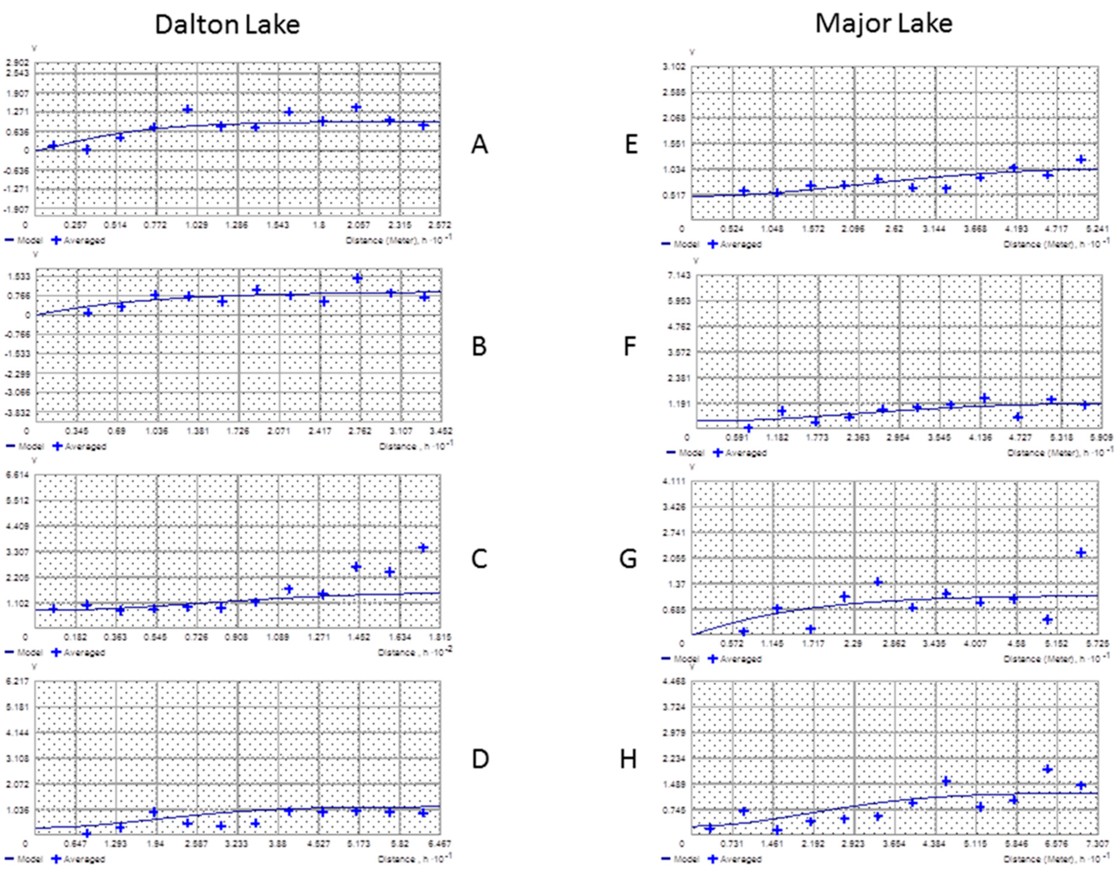
To determine the best accuracy of three common interpolation methods, we ran the data through ArcMap using Inverse Distance Weighted (IDW), spline and ordinary kriging. Two of these interpolation methods, IDW and spline, have been classified as “Non-Geostatistical Interpolators” where the ordinary kriging strictly functions through geostatistical methods [21]. Interpolation with IDW is based on value estimates being determined from linear combinations of values at sampled points and then weighted by the distance from the point of interest to sampled points. One main assumption with IDW is that the further the surface is from the known value the less similar it becomes. Near points will have greater influence on a particular spot than values further away. During IDW interpolation, the weight placed on the value is in inverse proportion to its spatial distance from the target locale. Spline is performed through local polynomials that describe small line segments that are fitted so that they form a smooth curve. The smooth curve produced from spline interpolation is forced through the set of known points to estimate the unknown values. Kriging has been classified as a geostatistical interpolator where the estimation of residuals is determined from the mean. The number of sampled points used in estimation of the mean is determined through the semi-variogram. Ordinary kriging methods were used in this study. During the process of kriging, different steps need to be observed and include plotting the experimental variogram, choosing the models that have the best shape, and plotting the model against the variogram [21]. Semivariograms used in this study are presented (Figure 1). The subfigures represent the semivariances of lags between sample points and the fitted smooth curve that best describes the sediment depth features while ignoring point-to-point fluctuations. This analysis provided a background for the best interpolation method for sediment data in the Black Hills and if any of them would be preferred during later stages of the study.

For the second objective, the data were randomly subsampled in triplicate at levels of 50%, 33% and 25% of the total dataset. Each of the selected points were identified within ArcMap as to the exact interpolated value with the identify tool and these values were compared to the sediment value originally measured in the field. Accuracy was determined using Root Mean Squared Error (RMSE) for each interpolation method and for each replicate. Correlation coefficients (r²) are noted to be misleading model performance measures [1,5]. The RMSE was used to determine the residual differences with the lower value exhibiting the greater accuracy [20]. RMSE was calculated using formula given by Li and Heap [21]. We were able to determine a RMSE for the full sample because these data are determined after interpolation and were comparing with “known” data from field measurements.

Figure 1. Semivariograms for total sample (A and E), 50% subsample (B and F), 33% subsample (C and G) and 25% subsample (D and H) of sediment data from Dalton Lake and Major Lake, South Dakota. Crosses are average measures of the empirical values of the semivariogram cloud.

Figure 1. Semivariograms for total sample (A and E), 50% subsample (B and F), 33% subsample (C and G) and 25% subsample (D and H) of sediment data from Dalton Lake and Major Lake, South Dakota. Crosses are average measures of the empirical values of the semivariogram cloud.

The estimates of volume were determined within ArcMap using the “Cut/Fill” tool. These estimates were determined from IDW interpolation used in objective one and at each of the smaller subsamples of IDW used in objective two. To determine the total volume, two sets of calculations were required. Firstly, a field where only the top of the sediment was measured was added to the dataset. This data was later used to develop a volume of water in the lake. Secondly, a field was calculated where the total depth of the sediment and the water depth gave an estimate of the total lake volume. From a simple graphing procedure, comparisons of each subsample and estimates to the overall sediment volume were determined in order to resolve the samples size needed. We originally decided to use IDW, spline and kriging interpolation methods because of familiarity, available software and past work [19].

From this study, a recommendation for the most accurate interpolation method for sediment surveys in the Black Hills was presented. This study determined if lower amounts of data, equaling lower costs, could occur while obtaining the same relative accuracy. In addition, the results of this work would provide researchers with a background for future work while also giving some guidance towards costs associated with fieldwork. These are topics not recorded in literature and are important for future sediment studies.

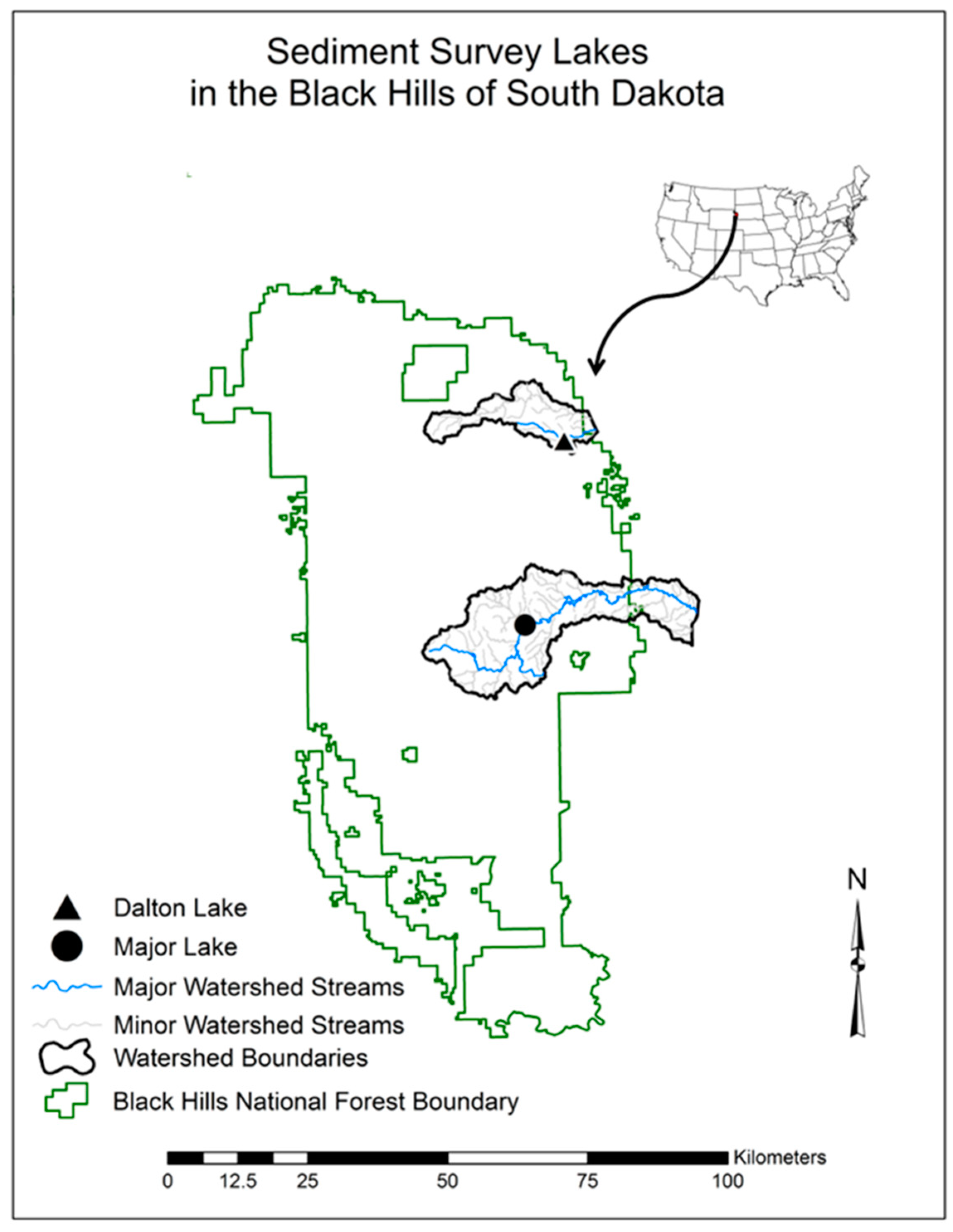
Two study lakes used in this study reside within the boundary of the Black Hills National Forest (BHNF) with land management directed by the USFS (Figure 2). Dalton Lake (1.2 ha) and Major Lake (1.2 ha) were chosen for analysis of interpolation accuracy.

Figure 2. Map of sample area in the Black Hills of South Dakota. Triangle is the location within the Elk Creek Watershed where Dalton Lake is located. The circle is the location where Major Lake is located within the Spring Creek Watershed.

Figure 2. Map of sample area in the Black Hills of South Dakota. Triangle is the location within the Elk Creek Watershed where Dalton Lake is located. The circle is the location where Major Lake is located within the Spring Creek Watershed.

Even though each lake is of equal size, the total number of sample points was slightly different due to the shape of the lakes. The watersheds of these lakes are heavily forested with ponderosa pine (Pinus ponderosa) along with stands of Black Hills spruce (Picea glauca), aspen (Populus tremuloides) and bur oak (Quercus macrocarpa). Each lake has impacts in their respective watersheds that have affected the amount of sediment inputs into the inlet areas and other parts of the lake. Having lakes in two watersheds was important so that no one event, such as runoff after a forest fire, would be a potential major influence of sediment into sampled waters. Dalton Lake is more rural in nature with anticipated impacts primarily of road building and forestry practices where Major Lake is urban, actually residing in the town of Hill City, SD, and has obvious impacts of road building, lawn runoff and hobby farming within its watershed.

3. Results and Discussion

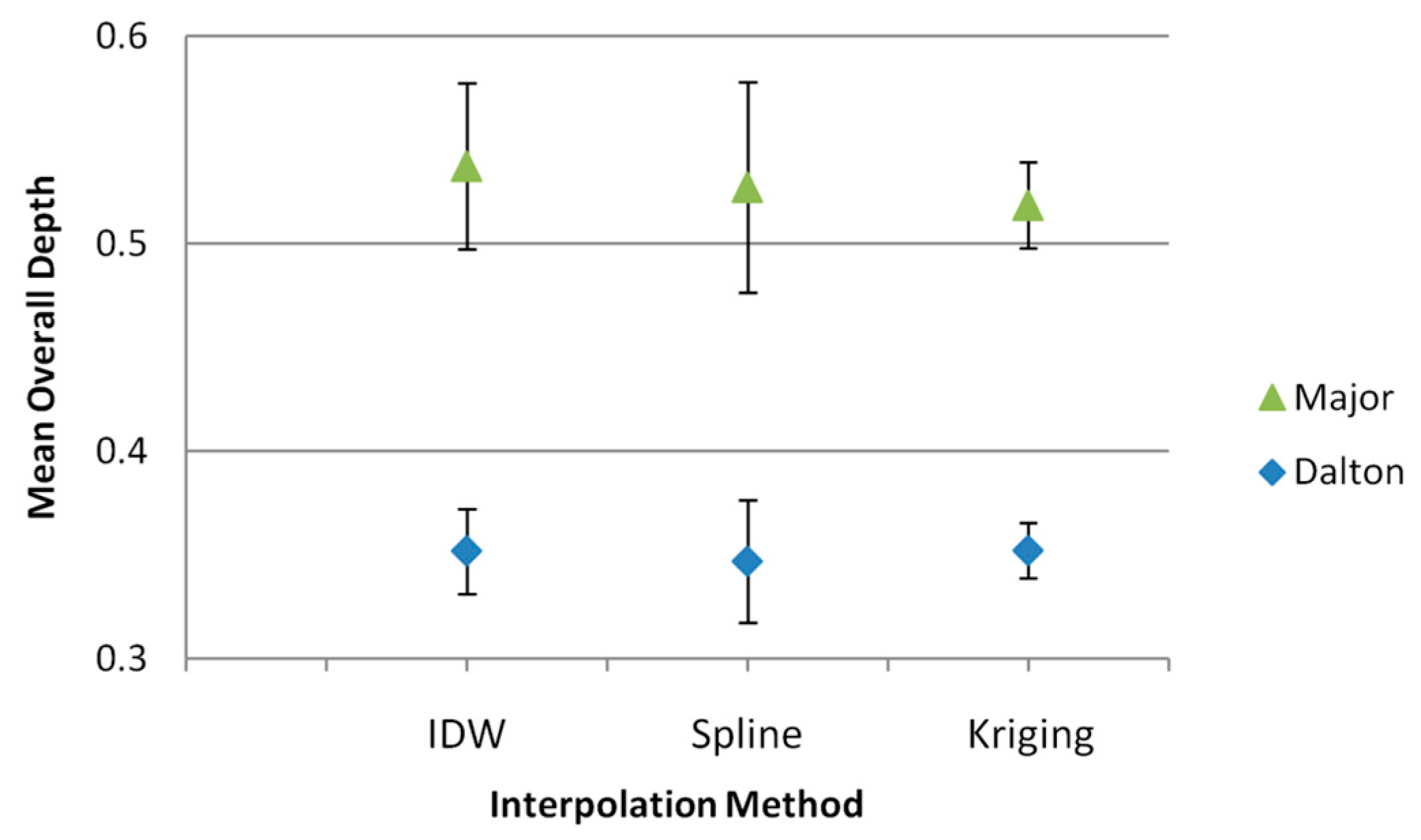
A total of 73 sample points were taken at Dalton Lake. The mean overall depths interpolated with any of the three methods tested in this study were not different from one another (One-way ANOVA (F(2213) = 0.07, p = 0.932) (Figure 3). Confidence intervals varied greatest with Spline, then IDW and finally Kriging. At Major Lake, a total of 81 samples were taken at individual points throughout the lake. The three tested interpolation methods were also similar in regards to their overall means and confidence intervals (One-way ANOVA (F(2234) = 0.13, p = 0.878). The variances in confidence intervals from Major Lake were similar to those from Dalton Lake; Spline had the greatest degree of dispersion, IDW was intermediate and kriging had the lowest confidence intervals of the methods tested.

Figure 3. Mean sediment depths of all data interpolated from two Black Hills lakes. Error bars are 95% confidence intervals.

Figure 3. Mean sediment depths of all data interpolated from two Black Hills lakes. Error bars are 95% confidence intervals.

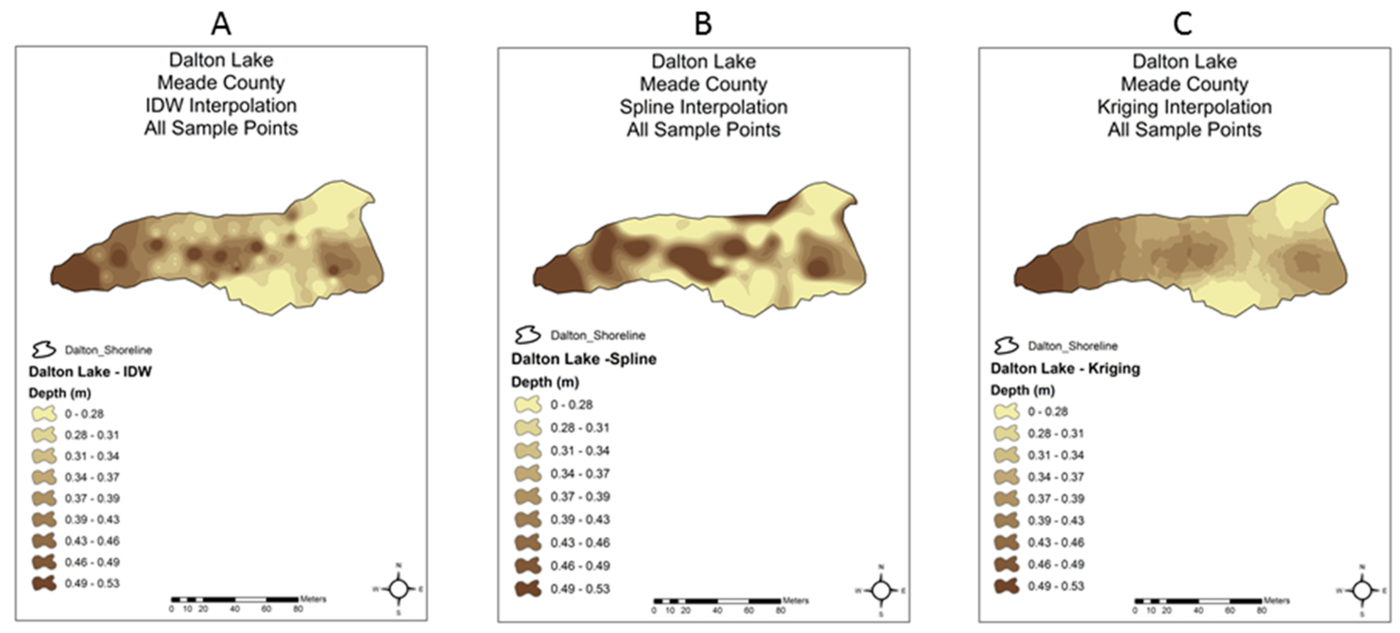
As expected, greater amounts of sediment are located nearer to the inlets than more distant areas (Figure 4). Matyas and Rothenburg detailed how the sediment was likely to be distributed in reservoirs, and observations from our two study lakes verified similar trends [8]. There may be some additional, localized sediment impacts, but much of the sediment appeared to be influenced by aspects within each watershed. Road building along the stream corridor above Dalton Lake may be having an impact on the overall sediment loading within the lake. A plume of sediment starts near the inlet and continues almost the full length of the lake towards the dam face (Figure 4). This observation was noted in all three interpolation methods tested at Dalton Lake.

In Major Lake, the sediment deposition differed from Dalton Lake. Where Dalton Lake sediment appeared to occur from inlet inputs and dispersed towards the dam, Major Lake had sediment levels higher along both sides of its longest edge (Figure 5). The deposition of sediment may possibly be from original sloughing of the shoreline, from unknown currents within the lake itself or from urban effects. Neither lake has a stream flow gauge above the lake so exact flow pulses that would contribute to either unique sediment pattern are unknown. Additional inputs of sediment showing an initial influx from the inlet area and spreading to the dam were measured and displayed with all three interpolation methods.

Figure 4. Sediment maps of Dalton Lake within the Black Hills of South Dakota using IDW interpolation to depict extent and distribution of sediment within the lake. Inverse Distance Weighted is identified with the subset letter (A), Spline is identified with the subset letter (B) and kriging is identified with the subset letter (C).

Figure 4. Sediment maps of Dalton Lake within the Black Hills of South Dakota using IDW interpolation to depict extent and distribution of sediment within the lake. Inverse Distance Weighted is identified with the subset letter (A), Spline is identified with the subset letter (B) and kriging is identified with the subset letter (C).

Figure 5. Sediment maps of Major Lake within the Black Hills of South Dakota using IDW interpolation to depict extent and distribution of sediment within the lake. Inverse Distance Weighted is identified with the subset letter (A), Spline is identified with the subset letter (B) and kriging is identified with the subset letter (C).

Figure 5. Sediment maps of Major Lake within the Black Hills of South Dakota using IDW interpolation to depict extent and distribution of sediment within the lake. Inverse Distance Weighted is identified with the subset letter (A), Spline is identified with the subset letter (B) and kriging is identified with the subset letter (C).

4. Accuracy of Interpolation Methods

To determine the best accuracy of the three interpolation methods, Root Mean Squared Error (RMSE) was used. A high RMSE value indicates that the predicted value (from each interpolation method) produced values that were further away from the mean or regression line [20].

In both study lake examples, the spline interpolation method produced the lowest RMSE from the observed to the predicted depths (Table 1). Spline interpolation has a greater emphasis towards small-scale features and uses piece-wise functions of few points at a time to render surfaces that can show predictions that are close to original values [22,23]. Errors of spline interpolation can exist in the process as the spline smoothes out sharp edges which may be found with point data. In this study, sediment measures were collected as point data and the natural smoothing function of spline interpolation based off these locations provided the most consistent accuracy. Spline did not suffer from the smoothing function in these two sample lakes and was more accurate than IDW and kriging interpolation methods. IDW interpolation works on the principle that phenomena closer together will be more similar than things farther away [2]. The authors believe that this is the case with sediment, as measures would be like a gently moving sheet that decreases away from the general impact of the event. In the case of sediment within a lake, the event could be a drastic change during a flood event or long-term impacts that greatly influence the general nature of phenomena distribution. Residing only slightly behind spline in regards to accuracy, IDW does hold some promise as an interpolation process for sediment surveys in the Black Hills.

Kriging was the most inaccurate of the three interpolation methods tested. At both sample lakes, kriging interpolation had the highest RMSE and was extremely high at Major Lake where the value was more than double of IDW and spline interpolation methods. Hengl discussed how kriging interpolation has two principle assumptions: that the target variable is stationary and that it adheres to a normal distribution [24]. While the distribution of sediment may not significantly change while measurements are being taken, it may be the case that sediment data are not normally distributed. As discussed earlier, sediment amounts were noted as being much greater at inlet areas than in other areas of the lake. Stein et al. and Voltz and Webster both suggested that distinct and sharp changes can cause problems with interpolation methods [23,25].

5. Accuracy of Subsamples

Typically, researchers assume that having more data provides a more accurate interpolation result. Li and Heap suggested there might be a “threshold” beyond which increasing the sample size does not improve estimation accuracy [20,21]. In this study, we pressed to find if there was a trade-off between effort expended and accuracy of results when using sediment data in the Black Hills.

Table 1. Root Mean Squared Error of full sample, 50%, 33% and 25% subsamples in three trials of sediment data from Dalton Lake and Major Lake.

Lake	Full Sample RMSE	50% RMSE				33% RMSE				25% RMSE
		Trial 1	Trial 2	Trial 3	Mean	Trial 1	Trial 2	Trial 3	Mean	Trial 1	Trial 2	Trial 3	Mean
Dalton Lake
IDW Spline Kriging	0.0706	0.0756	0.0736	0.0700	0.0731	0.0683	0.0851	0.0713	0.0749	0.0824	0.0819	0.0842	0.0828
	0.0459	0.0835	0.0663	0.0867	0.0788	0.0576	0.0953	0.0775	0.0768	0.1029	0.0761	0.0832	0.0874
	0.0942	0.1012	0.0930	0.0944	0.0962	0.0867	0.1068	0.0885	0.0940	0.0972	0.1034	0.1074	0.1027
Major Lake
IDW Spline Kriging	0.0691	0.0782	0.0887	0.0644	0.0771	0.0462	0.0385	0.0611	0.0486	0.0976	0.0439	0.0461	0.0625
	0.0589	0.1599	0.1047	0.0818	0.1155	0.0580	0.0879	0.0819	0.0759	0.1054	0.0778	0.0686	0.0839
	0.1735	0.1524	0.1855	0.1695	0.1691	0.1684	0.1408	0.1802	0.1631	0.1897	0.1700	0.1592	0.1730

Table 1. Root Mean Squared Error of full sample, 50%, 33% and 25% subsamples in three trials of sediment data from Dalton Lake and Major Lake.

Lake	Full Sample RMSE	50% RMSE				33% RMSE				25% RMSE
		Trial 1	Trial 2	Trial 3	Mean	Trial 1	Trial 2	Trial 3	Mean	Trial 1	Trial 2	Trial 3	Mean
Dalton Lake
IDW Spline Kriging	0.0706	0.0756	0.0736	0.0700	0.0731	0.0683	0.0851	0.0713	0.0749	0.0824	0.0819	0.0842	0.0828
	0.0459	0.0835	0.0663	0.0867	0.0788	0.0576	0.0953	0.0775	0.0768	0.1029	0.0761	0.0832	0.0874
	0.0942	0.1012	0.0930	0.0944	0.0962	0.0867	0.1068	0.0885	0.0940	0.0972	0.1034	0.1074	0.1027
Major Lake
IDW Spline Kriging	0.0691	0.0782	0.0887	0.0644	0.0771	0.0462	0.0385	0.0611	0.0486	0.0976	0.0439	0.0461	0.0625
	0.0589	0.1599	0.1047	0.0818	0.1155	0.0580	0.0879	0.0819	0.0759	0.1054	0.0778	0.0686	0.0839
	0.1735	0.1524	0.1855	0.1695	0.1691	0.1684	0.1408	0.1802	0.1631	0.1897	0.1700	0.1592	0.1730

Determining if there was a difference when sample size was taken into account, triplicate random samples (50%, 33% and 25%) were taken from each lake. RMSE values from this portion of the study showed some variability between lakes (Table 1). In all but one of the random samples (Major Lake 50%, Trial 1), spline and IDW were more accurate than kriging. RMSE values indicated that in many cases IDW subsamples were more accurate than spline interpolation. This is a slight contradiction to the overall data where we previously determined that spline was overall the most accurate interpolation with sediment data from these two lakes. Even in the full sample study, IDW was close to spline in many instances. An example of this near similarity occurred with the subsamples from Major and Dalton Lakes. In these two cases, the RMSE value for 25% (using IDW interpolation) was relatively similar to that of the 50%.

The spline interpolation method allows analysts to differentiate between smooth curves or tight straight edges between measured points. Spline interpolation often produces results that are visually appealing. Spline interpolation can also have different minimum and maximum values than the actual dataset. There may be a higher degree of sensitivity towards single outlier data points, and thus spline normally performs better when there is low variance within the data [26].

Spline interpolation was intermediate in accuracy between subsample datasets (Table 1). In two trials (Major Lake 50%, Trial 1, Dalton Lake 25%, Trial 1), RMSE values exceeded those of both IDW and kriging interpolation. Often spline was intermediate between IDW and kriging in regards to accuracy in each subsample. Dalton Lake and Major Lake had their lowest RMSE value with the 33% spline subsample.

Kriging was the third interpolation method used in this portion of the study. Webster and Oliver noted that sample sizes >50 were needed to reduce erratic behavior when kriging interpolation was used [27]. Other authors found that, in all but a few cases, there was a general increase in performance for many kriging methods when sample sizes were increased [28,29]. Conversely, Bourennane et al. thought that there was little change with sample size in kriging interpolation and that one could obtain accurate results with a sample size as low as 40 [30]. Kriging had the highest RMSE of all subsample when 25% of the points were used (Dalton Lake—Trial #3, Major Trial #1).

We found one general trend held constant throughout the three-subsample levels: the RMSE values did not increase as samples sizes decreased (Table 1). This trend was seen at Dalton and Major Lakes where the lowest RMSE was observed with the 33% subsample (Trial #1) or the 25% (Trial #2) subsample, respectively. The 50% subsample did not have the lowest RMSE value at either of these lakes. We could speculate that there were errors within the measurement procedures, yet these same procedures produced sediment estimates that were similar to “Total Station GPS” measures after sediment was removed.

The variability of RMSE did not show the anticipated trends of increasing RMSE values with the lower sample sizes in all cases (Table 1). The fewer samples would be a tradeoff due to less time required to collect data and thus a lower cost. There was only one increase of RMSE with smaller sample sizes in this portion of the study as shown by the slight increases of average values.

Trends of kriging interpolation are unclear. Kriging had the highest RMSE in all but two (Dalton Lake—25%—Trial #1, and Major Lake—50%—Trial #1) of all subsamples in this study. Data from Dalton Lake were the most consistent of either sampled waters when kriging interpolation was used.

6. Volume Comparisons

The third focus of this research incorporated findings of the previous two portions of the study with the purpose of determining if fewer samples would produce similar results. An estimate of sediment volume was determined for each lake and the results of data subsets were determined with subsamples of 50%, 33% and 25% using IDW interpolation (Table 2). It would be expensive if one were to reach the unrealistic goal of removing all of the estimated sediment; however, for comparative purposes these values provide a good comparison.

In both Dalton and Major Lakes, the effect of sample size was evident. As less data were used in the interpolation process, their volume estimates tend to drift further away from the full sample estimate. In only one instance (Dalton Lake, 33%) did this trend deviate from the tendency.

Table 2. Estimated volume of sediment (in cubic meters) and subsample estimates using IDW interpolation from two Black Hills ponds.

Percent of Sample	Estimated Volume (cu/m)
	Dalton Lake	Major Lake
Total	3435	8781
50%	3129	8327
33%	3205	7561
25%	2160	6371

Table 2. Estimated volume of sediment (in cubic meters) and subsample estimates using IDW interpolation from two Black Hills ponds.

Percent of Sample	Estimated Volume (cu/m)
	Dalton Lake	Major Lake
Total	3435	8781
50%	3129	8327
33%	3205	7561
25%	2160	6371

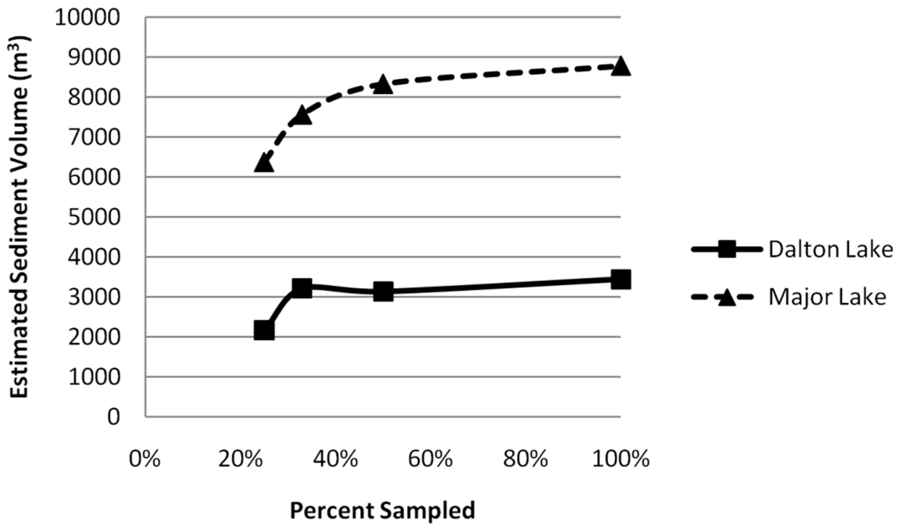
Previous we had smaller random subsamples providing interpolation accuracy representative to the greater sample size. To further examine these comparisons, we determined similarity through a simple graphing process. Graphing data from the whole sample and three subsamples (50%, 33% and 25%) based on the amount of sediment each predicted eventually produces a gradual sloping line (Figure 6). The asymptote of the plotted line shows only a slight increase after a sample approximately between 40%–50%. The data is displayed for both sample waters, but is more directly observed from Major Lake rather than at Dalton Lake. We originally assumed that predicted amounts of sediment would be more accurate with greater sample size, but the difference diminished when values exceeded 50%.

7. Summary and Conclusions

The first part of this project was to determine the accuracy of three interpolation methods based on how well they predicted the values at the known points. The best method produced the least error as measured by RMSE. In all of the sample waters, spline had the lowest RMSE, with IDW being a close alternative. Kriging ranked third in accuracy for point value prediction.

Kriging interpolation has been noted as being an accurate method in several studies, but was a poor performer in our study when RMSE values were compared [3,24,31,32]. Based on regionalized variable theory, the semi-variogram must be stationary over the area of interest and that the data is normally distributed [33]. These two issues may have influenced the outcome of the kriging RMSE values in our study. Further efforts to model different semi-variograms may improve the results obtained from the kriging algorithm.

Figure 6. Plot of sediment predicted by differing sampling amounts from two sample lakes in the Black Hills of South Dakota.

Figure 6. Plot of sediment predicted by differing sampling amounts from two sample lakes in the Black Hills of South Dakota.

Our effort to determine how many sample points are needed across these two study lakes was undertaken for more efficient sampling and potential cost savings. The methodology used for field collection requires personnel to commit to assisting for several days. If this fieldwork can be reduced while still obtaining similar results, then money in the form of time expended could be saved during data collection. Analysis for this aspect came from two different processes.

RMSE was again employed as a measure of interpolation accuracy, but in this case, it was with the subsamples (50%, 33% and 25%). Information from these tests was inconclusive. There was an original premise that there would be greater accuracy when more sample points were taken. We found that after approximately 40%–50% of our sample sizes, there was little overall improvement in the estimation of sediment volume. This study showed the importance of having the best accuracy especially when one considers the impact these could have on prioritization of projects and project amendments.

Throughout this study, many of the interpolation methods suffered in managing higher sediment values. When values were low or at least consistent, the interpolation methods all functioned well, with spline or IDW consistently the best alternatives. Kriging did well in some instances, but accuracy values suffered compared to those from other interpolation methods used. Subsample analysis showed that there were differences when the smaller samples were used. It is recommended to capture as much data as possible when performing sediment surveys in the Black Hills to ensure the most accurate estimates, but samples can be reduced and costs saved if it means fewer trips to gather data.

The results of an interpolation study can be considered in a step-wise fashion. One result of the process is normally a map which depicts the phenomena. If a researcher wants to judge the methods simply by visual means (i.e., appealing curvature of contour lines), then the results may look nice but could have poor representation in analysis of variables. It is important to apply the appropriate interpolation methods when developing surfaces as it may impact later modeling and analysis. In this study, the outcome was not simply to achieve an appealing map, but the results have a real world application. The application of this work was to provide an estimate of sediment volume. These conclusions were forwarded, along with a map of sediment distribution, to habitat biologists and administrators. This information is used for project prioritization and for more accurate private contractors bidding.