Abstract
This research examines the impact of climate and land use change on watershed hydrology. Seasonal variability in mean streamflow discharge, 100-year flood, and 7Q10 low-flow of the East Fork Little Miami River watershed, Ohio was analyzed using simulated land cover change and climate projections for 2030. Future urban growth in the Greater Cincinnati area, Ohio, by the year 2030 was projected using cellular automata. Projected land cover was incorporated into a calibrated BASINS-HSPF model. Downscaled climate projections of seven GCMs based on the assumptions of two IPCC greenhouse gas emissions scenarios were integrated through the BASINS Climate Assessment Tool (CAT). The discrete CAT output was used to specify a seed for a Monte Carlo simulation and derive probability density functions of anticipated seasonal hydrologic responses to account for uncertainty. Sensitivity analysis was conducted for a small catchment in the watershed using the Storm Water Management Model (SWMM) developed U.S. Environmental Protection Agency. The results indicated higher probability of exceeding the 100-year flood over the fall and winter months, and a likelihood of decreasing summer low flows.
1. Introduction
Floods, droughts and other weather-related extremes have inflicted, and are expected to inflict, growing costs on society [1,2,3,4,5]. According to the National Climatic Data Center of the National Oceanographic and Atmospheric Administration, over the past 30 years weather and climate-related disasters caused to communities in the U.S. total standardized losses in excess of $750 billion [6]. In 2011 alone, the estimated total damage cost due to wildfires, droughts and unprecedented flood events in the U.S. exceeded $52 billion [6]. Records of climatic variability and forecasts generated by climatic models provide decision-makers with the capability to assess risks of future conditions, develop scenarios, and increase resilience through practices and management options [3,7]. Coupled ocean-atmosphere General Circulation Models (GCMs) can be particularly useful in understanding future climates as they are capable of simulating climatic trends over decades [8]. Despite the advances in global climate modeling, considerable uncertainty exists with regard to regional variation and extent of future climatic impacts [9]. Arnell and Reynard [10] used a daily rainfall-runoff model and equilibrium vs. transient climate change scenarios to investigate variability in river flows in twenty one catchments in Great Britain. The study estimated an average river flow increase by 20% in wet periods and roughly 20% decrease in dry periods by 2050. Monthly flows were found to exhibit greater variability than annual flows with sharp increase in streamflow over the winter months. Inter-annual change was found to be less pronounced than inter-decadal streamflow variability [10]. Arnell [11] incorporated the UKCIP98 climate change scenarios into a calibrated hydrological model to investigate seasonal effects on mean monthly flows and low flows. The study compared natural multi-decadal variability to anthropogenic climate change effects and predicted increases in average monthly flows accompanied by substantial decreases in low flows in headwaters [11].
Rosenberg et al. [12] developed a comprehensive assessment of climate change impacts by regions and sectors for the conterminous U.S. Climate data for the analysis was provided by the Hadley/United Kingdom Meteorological Office (UKMO) general circulation model (GCM; HadCM2). Water yields for various time frames between 2030 and 2095 were modelled using the Hydrologic Unit Model for the United States (HUMUS). Overall, HadCM2 projections indicated wetter than normal conditions in the Pacific Northwest and the Ohio Valley and lower than normal water yields in the Lower Mississippi and Texas Gulf basins. Seasonal changes were also predicted including increased streamflow discharges in late winter and early spring [12]. Ficklin et al. [13] used GCM-projected variations in atmospheric CO2, temperature and precipitation to model impacts associated with climate change on evapotranspiration, water yield, streamflow, and water usage in San Joaquin Valley, California. The study predicted decrease in evapotranspiration by 37.5% and increases of water yield and stream flow by 36.5% and 23.5%, respectively. The study suggests high level of sensitivity in hydrologic endpoints with regard to potential changes in climatic conditions [13].
Denault et al. [9] explored the potential effect of future climate scenarios including increased rainfall intensity on urban stormwater peak discharges in a small catchment in British Columbia, Canada. The study examined the vulnerability of urban stormwater infrastructure to the effects of both urbanization and climate variability using rainfall-runoff simulations. The investigators found that upgrading existing infrastructure to projected streamflow alterations could be cost-efficient if incorporated in long-term water management planning [9]. Dessai and Hulme [14] argue that the implementation of successful water resource management strategies is often obstructed by the uncertainties associated with climate models predictions. The investigators suggest a framework to assess adaptation measures that are insensitive to ambiguities in climate model projections and can justify future investments in regional climate change adaptation strategies [14].
In addition to climate variability, conversion of land to urban uses is recognized as a major factor contributing to alterations in watershed hydrology [13,15,16,17]. Replacement of vegetation with impervious surfaces as a result of urban development affects microclimate and hydrology [16,18]. Urban development tends to remove vegetation and soil, increase imperviousness, and reduce natural infiltration capacity and ability to store floodwaters [15,17]. Alterations of a watershed’s hydrological characteristics due to urban development can significantly impact peak discharges, volume, and frequency of floods [13,16]. Over the past two decades, cellular automata (CA) models of urban simulation found numerous applications in practically every research area in the field of urban planning [18,19]. Researchers focus on the CA models in their explorations of the urban space because, for the most part, CA models are capable of conducting a number of previously intractable research tasks, such as modeling of spatial dynamics, simulation of micro-levels interactions, and capacity to predict emergent patterns [18,20]. Torrent et al. [19] developed a meta-simulation framework capable of running simulations incorporating both coarse scale (e.g., population growth) and fine scale (e.g., space and time) sprawl driving factors. Batty [20] explores a host of urban simulations models conceptually rooted in the complexity theory demonstrating their applicability to bottom-up stochastic temporal dynamics and phenomena associated with the processes of urban spatial evolution. Torrens et al. [20] represented a set of spatial determinants of sprawl on a geographic lattice to simulate the drivers of this well-known urban phenomenon.. Overall, research has demonstrated CA models applicability to spatially explicit representations of urban processes on a spatially referenced cellular lattice at incremental time steps governed by specific transition rules [21,22,23,24,25]. The CA model configurations have also increased in complexity. Onsted and Clarke [24] explored the applicability of SLEUTH to model the impact of regulatory policies such as voluntary differential assessment programs where lands are excluded from particular type of urban development in exchange of tax breaks. The approach successfully represented the shifting easement dynamics and contributed to improved goodness-of-fit statistics. Tang [26] used remote sensing and sub-cell fuzzy cellular automata to improve the accuracy of urban landscape change projections. Vancheri et al. [27] coupled the cell-based dynamics of cellular automata with multi-agent systems to analyze future real estate value and population distributions. Recent studies in cellular automata linked cell state transition in land use to associated activities such as residential development and employment [28]; and movement of capital and population [29]. Hansen [30] developed a scenario-based model framework which includes a land-use model, a runoff model, and a flooding screening model. Santé et al. [31] provide a detailed overview of recent developments in CA modeling.
This research links advances in urban growth modeling to downscaled climate projections to derive insights into the sensitivity of hydrologic response to changes in climatic conditions and level of urbanization. Land cover change is projected using a cellular automata (CA-Markov) model incorporating Markov transition probabilities and multi-criteria evaluation (MCE) [32]. Simulations from seven GCMs downscaled to individual Historical Climate Network (HCN) stations for the period 2010–2039 were obtained from the Consortium for Atlantic Regional Assessment (CARA) [33]. CARA’s website specifies simulated changes in temperature and precipitation under two of the IPCC commonly used future greenhouse gas emissions scenarios–A2 associated with rapid population growth and high energy use, and B2 associated with slower population growth and moderate energy use [33,34]. The sensitivity of hydrologic endpoints including mean seasonal streamflow (m3∙s−1), minimum (m3∙s−1), maximum (m3∙s−1), 100-year flood and 7Q10 low-flow (m3∙s−1) to climate drivers is examined using a calibrated hydrological model—the Hydrological Simulation Program–Fortran (HSPF) [35]. The seasonal effects of downscaled climate projections are incorporated into the model using the Climate Assessment Tool (CAT) built within the BASINS-HSPF modeling framework [7,36]. BASINS (Better Assessment Science Integrating Point and Nonpoint Sources) is a software package which combines the functionality of Geographic Information Systems (GIS) with state-of-the-art hydrological models and assessment tools to support comprehensive watershed and water-quality studies and guide the design and implementation of effective management strategies [7].
2. Materials and Methods
2.1. Description of the Study Area
Sensitivity of watershed hydrology to climate and land use change was examined through a simulation using a calibrated HSPF model for the East Fork Little Miami River watershed (referred to as East Fork hereafter). The watershed encompasses the south-eastern portion of the Little Miami River sub-basin (USGS Hydrologic Unit Code #05090202) covering a land area of approximately 1300 square kilometers. East Fork watershed is designated an Exceptional Warmwater Fisheries Habitat by the Ohio EPA [32]. The watershed receives an average monthly precipitation of 8.9 cm. The average annual precipitation ranges from 101.6 cm to 109.2 cm. Most of the annual rainfall (roughly 60%) occurs over the spring and summer months. Figure 1 displays the location of the study area in south-western Ohio.
According to the 1990 decadal census, the population of the Cincinnati-Middleton, OH-KY-IN Metropolitan Statistical Area (MSA) was 1.85 million. By 2000, the population increased to 2.01 million. Over 2.2 million currently reside in the OH-KY-IN MSA. Over a twenty-year period between 1990 and 2010, Hamilton County where the City of Cincinnati is located, lost almost 64,000 residents. At the same time, counties to the north and east of Cincinnati saw considerable increases in their population. Warren County increased its population by almost 100,000 people (or, 100%). Butler increased its population by 80,000 people (or, 70%). Clermont County, where the Lower East Fork Little Miami River watershed is located, gained 50,000 people which is an increase of over 30%.
The western portion of the watershed, which drains lower East Fork, is undergoing rapid suburbanization due to its location nearby the City of Cincinnati [32]. The prevailing urban development pattern is low-density residential with scattered commercial and industrial uses along major highways. In recent years, development moving in from the west led to increased population densities in the areas along US-50 and state routes 32 and 131. The construction of interchanges and extensions along the SR-125 and SR-32 corridors opened access to previously undeveloped sections in the lower and middle parts of the watershed. These areas are currently experiencing increased development pressure. Previous research has revealed that the rate of urban development in the East Fork watershed is affected by processes occurring at a larger scale [32]. In order to capture the dynamics of metropolitan development impacting the patterns of urbanization in the watershed, a cellular automata—Markov chains model was developed for the Cincinnati-Middleton metropolitan statistical area. The demographic transitions in the area in the past two decades suggest decline in population and employment densities within the urban core and rapid expansion of low-density greenfield development in the east, northeast and southwest directions [32]. Development trends in the East Fork watershed, located on the eastern fringe of the metropolitan area, are part of this overall exurban expansion.
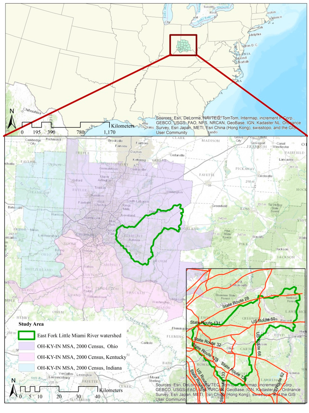
Figure 1.
Location of the Cincinnati Middleton OH-KY-IN MSA and the East Fork Little Miami River (EFLMR) watershed.
2.2. Conceptual Framework
Figure 2 depicts the conceptual framework and workflow of the study. The conceptual framework builds upon two primary dimensions—land cover change and projected climate variability to gain better understanding of the cumulative impact of these changes on runoff generation in an urbanizing watershed. The framework incorporates advanced land cover modeling techniques based on cellular automata and Markov chain probability and hydrological modeling using BASINS-HSPF and the Climate Assessment Tool (CAT) [36]. Projected 2010 land cover was validated using the 2010 parcel data for Clermont and Brown counties, Ohio. The hydrologic model of the watershed was calibrated and validated using the Root Mean Square Error (RMSE) and plotting observed versus simulated values. Since the climate model projections largely disagree on both the direction of change (increase/decrease) in precipitation and its magnitude, a Monte Carlo simulation was conducted to evaluate uncertainty in modeled results and estimate probability of exceedance of low flows (7Q10) and 100-year flood. The seasonal projected maximum and minimum precipitation were used as the basis of the climate scenarios. The initial results indicated a relatively modest magnitude of change which pointed out the need to rethink the scale of analysis. EFLMR is a relatively large watershed. The eastern sub-watershed is rapidly developing but still remains a relatively small portion of the East Fork Little Miami River watershed as a whole. The western portion including the headwaters is largely undeveloped consisting mainly of forested areas, pastures and agricultural land. The hydrological model was calibrated for the entire EFLMR watershed which explains the relatively modest magnitude of change (most of the area is undeveloped and this offsets the changes occurring in a small sub-watershed). To rectify for this and develop a better understanding of the changes occurring in the eastern portion of the watershed, one catchment was extracted from the eastern portion of the watershed as a separate unit of analysis. Further analysis was conducted within this rapidly suburbanizing catchment to reveal impact on runoff generation under extreme events.
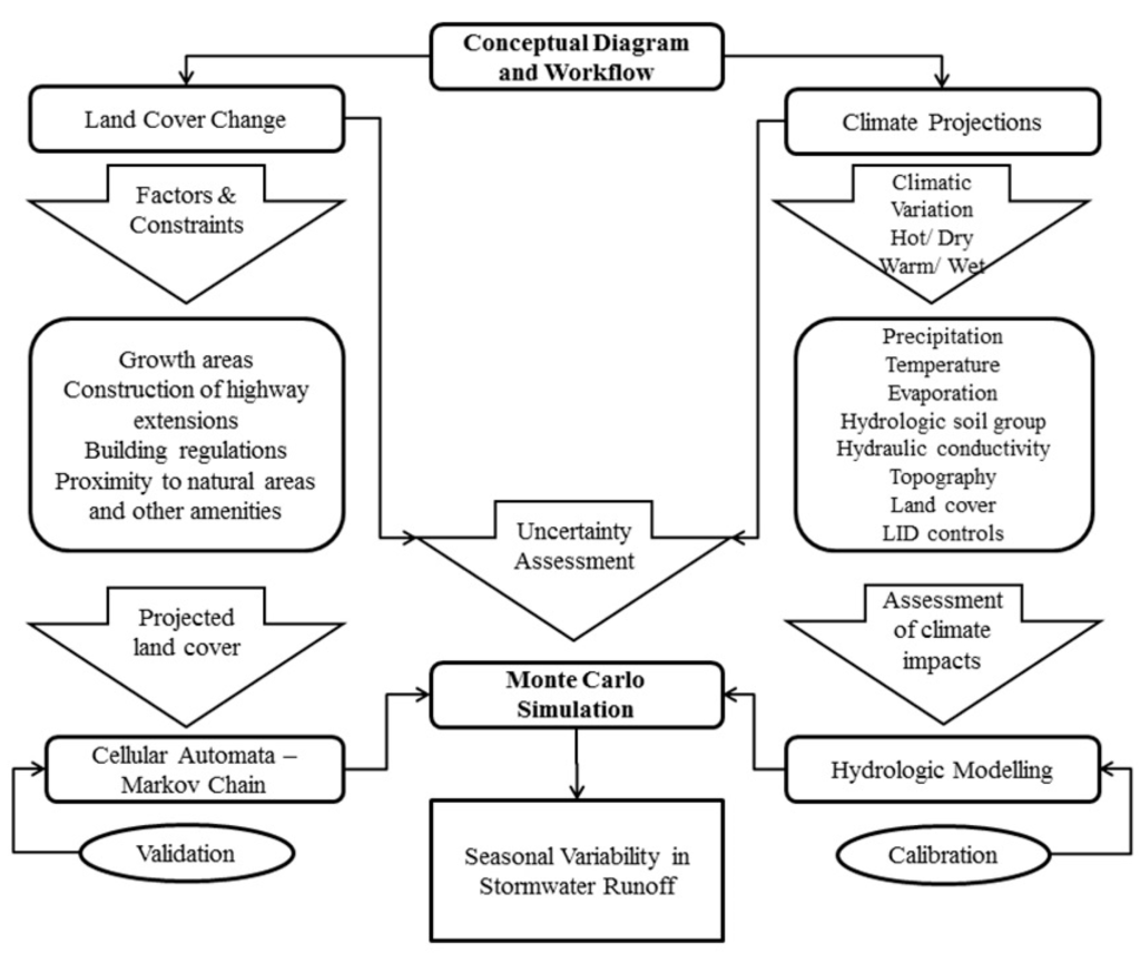
Figure 2.
Conceptual diagram and workflow.
2.3. CA-MARKOV Model of Land Cover Change
While in the past two decades urban growth CA models have remarkably improved their ability to achieve reliable simulations of urban morphologies, the exploration of coupling CA outputs with climate or other environmental models invites further investigation. Engelen et al. [37] developed a CA model as a component of a planning support system to examine the impact of climate change on land development of a Caribbean island. Inputs for the cellular automata (the micro-scale model) are first derived at the macro-scale based on four components: meteorological, demographic, economic, and land area requirement. Engelen et al. [37] used the model to study the impact of an increase in average temperature by 2 °C and the sea level rise of 20 cm on the land use patterns of coastal areas and the economy. The investigators simulated demand for land for various economic activities such as tourism, agriculture, exports, shopping and manufacturing. Arthur-Hartranft et al. [38] examine the modifications in vegetative cover, surface temperature and runoff resulting from simulated expansion of urbanized land in southeastern Pennsylvania. SLEUTH® urban growth model [23] was used to generate different scenarios of land cover alteration ranging from high impact development to more environmentally tolerant options that not only preserve but even extend vegetative cover. The land cover change images generated with the SLEUTH® model were then used as inputs in a hydrological model to develop a runoff response index under typical and atypical antecedent moisture conditions and investigate losses in the overall moisture storage due to urbanization. The study outlines important aspects of how the coupling of an urban CA model with environmental models can facilitate sustainable decisions regarding pace, scope, patterns and physical location of future urban development [38]. Liu et al. [39] generated various urban growth scenarios for the Pearl River Delta in southern China under alternative land use policies by integrating a cellular automata model with an artificial immune system technique that allows for dynamic parameterization of external drivers. Li et al. [40] combined ant colony optimization techniques with a cellular automata model to propose optimal zoning solutions for protected natural areas. The coupled model indicated improved performance compared to traditional models and resulted into a more compact urban form. Long et al. [41] incorporated spatial policy parameters into a constrained cellular automata model to evaluate an alternative development plan for the Beijing metropolitan area. The model was calibrated for four experimental urban forms using regionalized sensitivity analysis and evaluated for potential positive and negative impacts on the metropolitan area.
The historical land cover datasets used in the analysis were selected to be consistent with the climate data provided by CARA which was relative to a base period of 1971–2000 [34]. Past trends in landscape changes occurring in the study area were examined using the 1992 and 2001 National Land Cover Dataset (NLCD) datasets downloaded from the Multi-Resolution Land Characteristics Consortium [42]. Kappa Index of Agreement was used to validate and calibrate the land cover projections model [32]. The 2010 parcel data available through the Ohio Assessor and Property Tax Records was used to validate the 2010 land cover projection. For the purposes of simulating future development patterns, the original land cover/land use datasets were reclassified into seven land cover categories: urban high intensity, urban low intensity, woodland, cropland, wetlands, barren and water. They represented the initial “cell states” subject to change in the simulation process. A cellular automata—Markov transition probability model of land cover change was built within the CA-Markov module of IDRISI® Taiga GIS and Image Processing software [43]. The module inputs include a reclassified land cover grid representing the initial state of each pixel, a Markov transition probabilities matrix, a suitability image for each land cover/land use class subject to change, a contiguity filter for the cellular automata moving window, and a number of iterations [32,43].
The reclassified land cover images were used to generate the initial Markov transition probability matrix. They represented the observed frequencies of land cover class transitions during the initial observed period. The Markov transition probability matrix, created through the MARKOV module in IDRISI®, determined the likelihood of transition from the initial cell state (i.e., land cover class) to any other cell state based on past trends. Overall, four Markov transition probability matrices were computed for the analysis, each for a period of ten years.
The spatial patterns of the expected transitions were determined using a multi-criteria evaluation (MCE) approach which assigned a suitability score to each cell. MCE in IDRISI® requires a set of variables in the form of factors and constraints [43]. A constraining layer restricts transitions. Constraining layers were derived as separate Boolean images. An overlay by multiplication procedure was used to combine them into a composite constraint image. In this study, already developed land, streams, other water bodies, and road networks formed one set of constraints. Building regulations restricting construction on steep slopes because of slope instability, erosion, and landslide risk provided the regulatory basis for establishing another set of constraints. Separate constraining layers were developed for each simulated land cover class.
The degree of suitability of each cell for a particular objective was determined using input variables termed as factors. The choice of factors was determined based on the literature review [19,20,22,25,26] and statistical analysis. For the purposes of this analysis, factor variables included: (1) proximity to roads; (2) slopes below 25 percent (no restrictions based on the slope factor were applied to transitions to cropland, woodland, barren land and wetlands); (3) proximity to streams and water bodies; (4) proximity to protected natural areas and open space; and (5) proximity to growth areas, defined as areas that experienced substantial growth in population and employment between 1990 and 2000. Census tracts with increase in population density of more than 300 persons per square kilometer (2.5 standard deviations above the mean) and/or increase in employment density by more than 180 persons per square kilometer (2.5 standard deviations above the mean) were extracted and a new layer designated as growth areas was derived. The underlying assumption was that areas experiencing substantial growth in recent years would successfully attract future new development. Linear and sigmoidal fuzzy-logic functions were used to represent the distance decay. Various combinations of distance decay functions were applied to derive the composite suitability score for each of the seven land cover classes included in the analysis. These combinations determined the transition rules incorporated in the CA-Markov model. Assessment of the validity of the CA-Markov model was conducted using the Kappa Index to estimate the agreement between the 2010 projected land use and 2010 parcel data.
2.4. Assessment of the Impact of Climate Variability on Hydrologic Endpoints
The assessment of the potential impact of anticipated climate variability on watershed processes was conducted using a calibrated hydrological model and smoothed projections for the 2010–2039 change in mean annual and seasonal temperature and precipitation. Climatic data, derived from seven IPCC-supported GCMs, were provided by the Consortium for Atlantic Regional Assessment under two scenarios representing the mid-high (A2) and mid-low (B2) ranges of greenhouse gas emissions [44]. Both scenarios presume moderate levels of economic development. The A2 scenario assumes high rates of population growth, energy consumption, and land conversion while B2 represents a more environmentally friendly approach with moderate rates of population increase, energy use, and land cover change [34,44]. Table 1 provides a summary of the hydrological endpoints over a historical period of 35 years.

Table 1.
Monthly averages for the hydrologic endpoints values based on historical records 1969–2004 (Data Source: Weather Station OH335268 near Milford, Ohio, USA.
| Month | Hydrologic Endpoint Values Based on Historical Record 1969–2004 | ||||
|---|---|---|---|---|---|
| 100-Year Flood (m3 s−1) | 7Q10 (m3 s−1) | Maximum (m3 s−1) | Mean (m3 s−1) | Minimum (m3 s−1) | |
| January | 49.4 | 8.9 | 95.6 | 18.1 | 0.3 |
| February | 88.8 | 10.4 | 59.6 | 18.1 | 1.1 |
| March | 50.2 | 9.8 | 38.6 | 17.1 | 5.3 |
| April | 105.7 | 8.2 | 60.0 | 19.2 | 7.4 |
| May | 366.3 | 8.8 | 134.0 | 23.7 | 8.0 |
| June | 351.6 | 9.8 | 131.3 | 25.0 | 7.4 |
| July | 189.1 | 9.9 | 90.4 | 19.3 | 6.9 |
| August | 42.8 | 6.0 | 90.5 | 17.1 | 5.4 |
| September | 79.0 | 4.4 | 46.0 | 14.3 | 4.0 |
| October | 64.1 | 4.9 | 38.4 | 14.2 | 4.3 |
| November | 50.0 | 4.1 | 38.3 | 13.2 | 4.0 |
| December | 60.3 | 3.9 | 40.9 | 15.4 | 3.8 |
The Consortium for Atlantic Regional Assessment (CARA) provides historical records and climate projection data for 114 to individual Historical Climate Network (HCN) stations in the North Atlantic region and 67 near-by stations, 24 of which are located in Ohio. The HCN station at Hillsboro, OH (Historical Climate Network #333758, 39.21N, 83.62W) was selected for this analysis because of its proximity to the study area and appropriate elevation (approximately 290 m) which falls within the range of the highest and lowest elevation points observed in the watershed (380 m and 160 m, respectively). The climate projection data provided by CARA are in the form of deltas, or expected changes in the mean annual and seasonal temperature and precipitation (including respective standard deviations) relative to the base period, 1971–2000 [7,34]. Table 2 provides a summary of the downscaled projections from the seven general circulation models included in the analysis.
The Climate Assessment Tool (CAT) [36] incorporated in BASINS v.4 is a scenario generating utility which enables the user to adjust historical precipitation and temperature time series contained within BASINS Watershed Data Management (WDM) file according to expected changes [7]. For the purposes of this research, monthly times series subsets were aggregated by season and modified using the iterate changes approach to evaluate seasonal responses to future climate conditions (i.e., precipitation and temperature). The approach, also known as the delta method, consists of modifying historical data records by an array of projected changes, or deltas [7]. It offers a number of advantages including ease of implementation, capability of evaluating a wide range of potential outcomes, and consistency in preserving “any spatial or temporal structure present in observed weather records” ([7], pp. 2–3). Consequently, the delta method represents “a simple but effective form of spatial and temporal downscaling, whereby coarser scale climate change information is superimposed over more spatially (e.g., an individual weather station) and temporally detailed (e.g., daily or hourly data) historical observations” ([7], pp. 2–3).
Table 2.
Projected percent change in average annual and seasonal precipitation at HCN# 333758 (Hillsboro, OH) based on the outputs of seven GCMs for the period 2010–2039 (baseline 1971–2000).
| Scenarios/ | Deltas from General Circulation Models Output for 2010–2039 | ||||||
|---|---|---|---|---|---|---|---|
| Timeseries | CCCM a | CCSR b | CSIR c | ECHM d | HDCM e | NCAR f | GDFL g |
| A2 (mid-high) | Projected percent change in average precipitation over the base period 1971–2000 | ||||||
| Annual | 0.04 | −0.03 | −0.02 | −0.02 | 0.03 | 0.04 | 0.02 |
| Winter | 0.00 | 0.08 | 0.05 | −0.14 | 0.06 | 0.11 | −0.01 |
| Spring | 0.08 | −0.01 | 0.04 | −0.05 | 0.05 | −0.01 | 0.02 |
| Summer | −0.02 | −0.14 | 0.01 | 0.06 | 0.05 | 0.01 | 0.00 |
| Fall | 0.16 | 0.03 | −0.20 | 0.00 | −0.19 | 0.21 | 0.14 |
| B2 (mid-low) | Projected percent change in average precipitation over the base period 1971–2000 | ||||||
| Annual | 0.08 | 0.07 | 0.04 | 0.06 | 0.03 | −0.01 | 0.01 |
| Winter | −0.02 | 0.08 | 0.08 | 0.01 | 0.05 | 0.05 | −0.01 |
| Spring | 0.06 | 0.05 | 0.00 | −0.01 | 0.02 | −0.03 | 0.02 |
| Summer | 0.03 | 0.03 | 0.09 | 0.09 | 0.10 | −0.05 | −0.03 |
| Fall | 0.33 | 0.12 | −0.02 | 0.13 | −0.09 | 0.07 | 0.12 |
a CCCM—Canadian Centre for Climate Modeling and Analysis [45]b CCSR—University of Tokyo, Center for Climate System Research [46]c CSIRO—Australia’s Commonwealth Scientific and Industrial Research Organization [47]d ECHM—German High Performance Computing Centre for Climate and Earth System Research [48]e HADC—Hadley Centre for Climate Prediction and Research [49]f NCAR—National Center for Atmospheric Research [50]g GFDL—Geophysical Fluid Dynamics Laboratory [51]
The evaluation of watershed responses using BASINS CAT utility requires a calibrated HSPF watershed model. HSPF is a physically-based hydrologic model with capabilities to simulate flow and water quality processes using land cover/land use data, hourly meteorological inputs (e.g., hourly precipitation, solar radiation, evapotranspiration, and air temperature), and information on stormwater management practices [35]. For the purposes of this analysis, the National Elevation Dataset (NED) at 10 m resolution and the National Hydrographic Dataset downloaded from the National Map Viewer (USGS, http://viewer.nationalmap.gov/viewer/).
2.5. Sensitivity Testing
Sensitivity testing under various climate scenarios (hot/dry and warm/wet) for the near term period for a 20 year period (2010–2030) and various levels of imperviousness starting with the 2010 observed level of 31.2 percent was conducted for a portion of the Lower East Fork (near Milford). The Storm Water Management Model (SWMM) built within the USEPA stormwater simulator was used to conduct this portion of the analysis [52]. The model requires various inputs including hydrologic soil group, hydraulic conductivity, surface slope, land cover, topography, precipitation and evaporation time series, and low impact development (LID) controls. Ten scenarios were explored under various set of conditions. Outputs include infiltration (% rainfall), evaporation (% rainfall), runoff (% rainfall), average annual rainfall (in), average annual runoff (in), days per year with rainfall days per year with runoff, percent of wet days retained, smallest rainfall with runoff (in), largest rainfall without runoff (in), maximum rainfall retained (in).
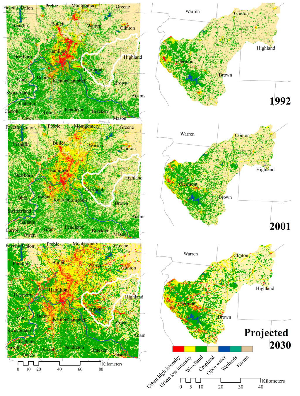
Figure 3.
The 1992–2001 land cover change derived from NLCD and the 2030 land cover projection.
3. Results and Discussion
3.1. Land Cover Change
The analysis of land cover changes occurring between 1992 and 2001 indicated that throughout the metropolitan area built-up land have increased by nearly 1200 square kilometers, or approximately 10 percent (Table 3). Urban area had mostly increased by encroaching on cropland, and to a lesser extent on woodland/open space. Figure 3 displays the reclassified land cover datasets for 1992 and 2001 as well as the projected 2030 land cover image. Throughout the same period the woodland/open space category was both gaining and losing area. The primary cause of these losses was the expansion of the urban development. The gains were likely due to establishment of conservation easements, expansion of protected areas, and secondary forest re-growth on land that was cleared but not rapidly developed. The trend analysis of the direction of the change associated with conversion of cropland confirmed that the most changes occurred in the northeast and east direction, including the East Fork watershed. According to the results of the CA-Markov urban growth model, the metropolitan urban land is expected to increase by approximately 15 percent between 2001 and 2010, 8 percent between 2010 and 2020, and some additional 7 percent between 2020 and 2030.
Table 3.
Summarizes the observed (1992–2001) and the projected land cover change (2001–2030) for the seven land use classes included in the simulation (area in square kilometers).
| OH-KY-IN MSA | 1992 | 2001 | Projected 2010 | Projected 2020 | Projected 2030 |
|---|---|---|---|---|---|
| Urban High Intensity | 361.38 | 377.71 | 538.97 | 700.70 | 860.72 |
| Urban Low Intensity | 662.94 | 1831.12 | 2335.50 | 2706.92 | 3029.08 |
| Woodland/Open space | 5440.65 | 5519.76 | 5942.51 | 6038.76 | 6098.52 |
| Cropland | 7360.33 | 6138.60 | 5061.85 | 4429.27 | 3884.77 |
| Water | 234.83 | 242.27 | 247.31 | 250.70 | 253.38 |
| Wetlands | 71.43 | 25.97 | 27.29 | 28.17 | 29.10 |
| Barren land | 18.10 | 14.22 | 12.95 | 11.88 | 10.92 |
| EFLMR Watershed | 1992 | 2001 | 2010 | 2020 | 2030 |
| Urban High Intensity | 10.35 | 14.74 | 29.19 | 29.21 | 85.37 |
| Urban Low Intensity | 39.80 | 117.48 | 135.45 | 169.48 | 263.89 |
| Woodland/ Open space | 328.17 | 417.42 | 420.31 | 420.38 | 397.01 |
| Cropland | 885.59 | 713.77 | 678.21 | 644.09 | 517.37 |
| Water | 12.79 | 12.80 | 12.75 | 12.75 | 13.00 |
| Wetlands | 2.34 | 2.03 | 2.44 | 2.44 | 2.52 |
| Barren land | 1.30 | 2.10 | 1.99 | 1.99 | 1.18 |
The trends in the land cover change processes observed at the metropolitan level were similar to those observed at the watershed level. In 1992, only 3.8 percent of the East Fork watershed area was urbanized. By 2001, the percentage of urban land increased to 132.2 sq.·km or 10.3 percent. Between 1992 and 2001, the East Fork watershed lost over 170 sq.·km of productive agricultural land. The CA-Markov model projection suggests that if the rates of change persist, by 2030 some additional 196 sq.·km of cropland would be converted to predominantly urban uses. This will include 85.4 sq.·km of urban high intensity land (i.e., industrial, commercial, transportation and high density residential uses). The change analysis indicated that woodland/open space increased between 1992 and 2001. Most of this increase was due secondary shrub/scrub regrowth on abandoned agricultural land. Some of this land was also converted to open space in the urbanizing areas.
3.2. Incorporating Downscaled Climate Projections in BASINS-HSPF
Kappa statistics were separately calculated for the agreement between observed and projected urban areas. The projected 2010 urban land use for the Lower and Middle East Fork was cross-tabulated with the residential, industrial and commercial land uses derived from the 2010 parcel data to assess the validity of the CA-Markov model (Figure 4). The overall Kappa statistic is 0.766, a very good agreement between observed data and modelled result. The area of the urban land use projected by the model was 143 sq.·km compared to the existing 149 sq.·km derived from the 2010 parcel data. Closer examination of the overlay on Figure 4 suggests that the model overestimated the extent of growth in the southeast part of the Middle East Fork while underestimating the amount of development in the northeast part of the Lower East Fork.
Meteorological data series associated with the weather station near Milford, OH (OH335268) were imported into Watershed Data Management (WDM) format using WDMUtil tool within BASINS v.4. The time series contained meteorological records from 03/31/1969 through 07/31/2004. Climate projection data for the period 2010–2039 summarized by season was downloaded from CARA’s website (Table 2). Historical streamflow base records from 1 January 1997 through 29 July 2004 obtained at the USGS monitoring gauge station at the watershed outlet in Perintown, Ohio (#03247500), were used to calibrate and validate the East Fork HSPF model (Figure 5). The calibration period covered 49 months (from 1 January 1997 through 31 December 2000) and was based on 1461 daily streamflow observations. The model was validated over a 43-month period (1 January 2001 through 29 July 2004) using 1306 daily streamflow observations. We derived a RMSE of 13.7 for the calibration period, and a RMSE of 20.6 for the validation period. The correlation coefficient between simulated and observed daily flow was found to be 0.986. Figure 5 presents the results from the calibration and validation procedures.
Adjustments to historical weather data using the delta method were computed using the operators specified by the “How to Modify” option of BASINS Climate Assessment Tool (CAT) [36]. The adjustments include re-computation of potential evapotranspiration using projected temperature change [7]. The deltas presented in Table 2, are incorporated in the hydrological model of the East Fork watershed using the stepwise approach suggested by USEPA [7]. The historical base record (1969 to 2004) was adjusted by constant multipliers based on the minimum and maximum projected seasonal changes from the climate models outputs.
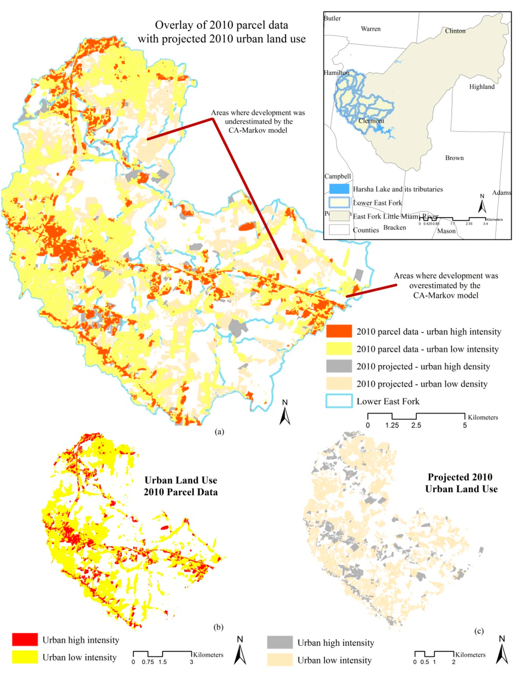
Figure 4.
Comparison of 2010 parcel data for the rapidly urbanizing Lower East Fork with the 2010 projected land use change. Top left, map (a) overlay of maps (b) and (c); Lower left, map (b) urban high and low density areas as derived from the 2010 parcel data; Lower right, map (c) projected urban high and low density areas.
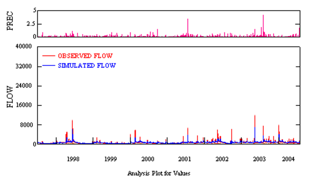
Figure 5.
Watershed hydrological model calibration and validation.
Table 2 displays the projected changes in precipitation by the year 2030 used in the adjustment of meteorological time series under scenarios A2 and B2. As Table 2 indicates, projected trends in future precipitation changes are not consistent across the models. CCCM [45] projects a 2 percent decrease while CCSR [46] projects an 8 percent increase in the average winter precipitation. Projections suggest that the average September through December precipitation changes vary from a reduction of 9% (HDCM) [49] to an increase of 33% (CCCM) [45] under scenario B2, and from a reduction of 20% (CSIRO) [47] to an increase of 21% (NCAR) [50] under scenario A2. The ECHM model [48] suggests a decrease in the average winter precipitation by 14% under scenario A2, while the NCAR model [50] projects an increase by 11%. Most models project an increase in average winter rainfall under scenario B2. CCSR model [46] suggests a 14-percent decrease in summer precipitation under scenario A2 while ECHM [48] suggest a 6-percent increase. Projections under scenario B2 suggest a 10-percent increase in summer rainfall (HDCM) [49] as well as a 5-percent decrease (NCAR) [50]. Similar trends are observed during the spring season (Table 2).
Minimum and maximum downscaled projection values across the seven general circulation models for each season were used as inputs to BASINS CAT to simulate deltas of expected change in precipitation patterns. A total of sixteen scenarios were generated, two for each season under each scenario. The BASINS CAT output suggested a decrease in winter, summer and spring low flows under both scenarios by the year 2030. However, more favorable conditions are likely to be observed under emissions scenario B2 which is expected to result in a lesser amount of decline of the 7Q10 low flows. The impact of climate and land use change on the 7Q10 low flow discharge (m3∙s−1) ranged from a reduction of 5% to a reduction of 35% during the summer season, a reduction of 6% to a reduction of 18% during the spring, and a reduction of 15% to a reduction of 52% during the winter months. The fall variation in 7Q10 discharge fluctuated from a reduction of 5% to an increase of 20%.
3.3. Monte Carlo Simulation
Due to the stochastic nature of the climate processes, the uncertainty inherent in climate and hydrological models, as well as the uncertainty associated with modeling sub-scale variation and heterogeneity [53], the discrete CAT output was entered into a series of Monte Carlo simulations to derive probability density and cumulative distribution functions of anticipated seasonal hydrologic response. An analysis of daily streamflow distributions revealed that the annual, spring, winter and fall values fit a log-logistic cumulative distribution function while the summer values followed a dagum distribution. A Kolmogorov-Smirnov (K-S) goodness-of-fit test was performed to determine how well the data fits the distributions. The results indicate that the calculated test statistic, D, was less than the critical value at the 0.01 significance level for all distributions. Thus, the null hypothesis with regard to the distributional form could not be rejected at this significance level for all estimated distributions.
The discrete output from the Climate Assessment Tool for minimum, maximum, 100-year flood discharge and 7Q10 low-flow (m3∙s−1) was used as a random number seed for sampling the specified log-logistic probability distributions using the Monte Carlo approach. Table 4 summarizes the results from the Monte Carlo simulation and probability analysis.
The results indicate that while the minimum and maximum temperature and precipitation change under scenario A2, there is a probability of 0.123 of exceeding the 100-year flood discharge. A projected 21% increase in precipitation over the fall months under scenario A2, yields a probability of exceedance of 0.177 for the 100-year flood discharge. A projected 33% maximum increase in precipitation over the same season is expected to yield a probability of exceedance of 0.254 of the same parameter under scenario B2. There is higher probability of decline below the baseline 7Q10 summer low flow. The results from the Monte Carlo analysis suggest a probability of 0.035 of a relative decrease in the summer 7Q10 flow under scenario A2, and a probability of 0.044 of a relative decrease under scenario B2 (the baseline values are mean of 8.6 m3∙s−1 and a minimum of 6.5 m3∙s−1). Similar patterns are observed for the spring low flows.
Table 4.
Results from the Monte Carlo simulation.
| Emissions Scenario | 100-Year Flood | 7Q10 | Mean | ||||
|---|---|---|---|---|---|---|---|
| Baseline (X) | (m3 s-1) | (m3 s-1) | (m3 s-1) | ||||
| Winter | 66.2 | 7.7 | 17.2 | ||||
| Spring | 174.1 | 8.9 | 20.0 | ||||
| Summer | 194.5 | 8.6 | 20.4 | ||||
| Fall | 64.4 | 4.5 | 13.9 | ||||
| Mid-High (A2) IPCC Emissions Scenario: X1 | Probability of Exceeding Baseline Values | ||||||
| Projected Change in Precipitation | P(X>X1) | P(X<X1) | P(X>X1) | ||||
| Min (ECHM) | −0.14 | Max (NCAR) | 0.11 | Winter | 0.123 | 0.029 | 0.077 |
| Min (ECHM) | −0.05 | Max (CCCM) | 0.08 | Spring | 0.045 | 0.013 | 0.022 |
| Min (CCSR) | −0.14 | Max (ECHM) | 0.06 | Summer | 0.036 | 0.035 | 0.010 |
| Min (CSIR) | −0.20 | Max (NCAR) | 0.21 | Fall | 0.177 | 0.009 | 0.085 |
| Mid-Low (B2) IPCC Emissions Scenario: X2 | Probability of Exceeding Baseline Values | ||||||
| Projected Change in Precipitation | P(X>X2) | P(X<X2) | P(X>X2) | ||||
| Min (CCCM) | −0.01 | Max (CSIR, CCSR) | 0.08 | Winter | 0.097 | 0.016 | 0.026 |
| Min (NCAR) | −0.03 | Max (CCCM) | 0.06 | Spring | 0.032 | 0.042 | 0.014 |
| Min (NCAR) | −0.05 | Max (HDCM) | 0.10 | Summer | 0.021 | 0.044 | 0.028 |
| Min (HDCM) | −0.09 | Max (CCCM) | 0.33 | Fall | 0.254 | 0.015 | 0.109 |
3.4. Sensitivity Analysis
Table 5 summarizes the results from the sensitivity analysis which includes three factors of variability: climate variability (hot/dry vs. warm/wet conditions), percent imperviousness (from the existing 30% to 90%), and various levels of low impact development practices such as disconnection of impervious surfaces, rain harvesting, rain gardens, street planters, infiltration basins, and porous pavement. The results indicate that LID controls can increase infiltration and reduce runoff volume even if the extent of the impervious surfaces increases by almost 60 percent (e.g., scenarios 1 and 2). The effect of the LID practices is particularly notable under warm and wet climatic conditions. Scenarios 7 and 8 demonstrate that under the same level of imperviousness (53.2%) under warn and wet climate, the full range of LID practices reduces the amount of runoff by 25% assuming similar evaporation rates.
Table 5.
Results from sensitivity analysis for two near-term climate scenarios with 20-year time span and various levels of development (% imperviousness) and LID controls.
| Climate Change Scenario | Hot/Dry/Near Term | Warm Wet/Near Term | ||||||||
|---|---|---|---|---|---|---|---|---|---|---|
| Percent Impervious | 31.20% | 53.20% | 53.20% | 90.00% | 90.00% | 31.20% | 53.20% | 53.20% | 90.00% | 90.00% |
| Wet Day Threshold (Inches) | 0.1 | 0.1 | 0.1 | 0.1 | 0.1 | 0.1 | 0.1 | 0.1 | 0.1 | 0.1 |
| LID control: | % of impervious area treated/% of treated area used for LID | |||||||||
| Disconnection | 10 | 10 | 10 | 0 | 10 | 10 | 10 | 10 | 0 | 10 |
| Rain harvesting | 0 | 0 | 2 | 0 | 0 | 0 | 0 | 2 | 0 | 0 |
| Rain gardens | 0 | 0 | 5 | 0 | 0 | 0 | 0 | 5 | 0 | 0 |
| Street planters | 10 | 10 | 10 | 0 | 10 | 10 | 10 | 10 | 0 | 10 |
| Infiltration basins | 0 | 0 | 10 | 0 | 0 | 0 | 0 | 10 | 0 | 0 |
| Porous pavement | 5 | 5 | 5 | 0 | 5 | 5 | 5 | 5 | 0 | 5 |
| Results: | Scenario 1 | Scenario 2 | Scenario 3 | Scenario 4 | Scenario 5 | Scenario 6 | Scenario 7 | Scenario 8 | Scenario 9 | Scenario 10 |
| Average Annual Rainfall (in) | 45.8 | 42.48 | 42.48 | 42.48 | 42.48 | 46.92 | 46.92 | 46.92 | 46.92 | 46.92 |
| Average Annual Runoff (in) | 18.27 | 19.1 | 13.06 | 32.89 | 27.1 | 15.97 | 15.1 | 15.01 | 36.96 | 30.82 |
| Days per Year With Rainfall | 82.34 | 80.79 | 80.84 | 80.79 | 80.79 | 85.00 | 80.79 | 84.94 | 84.99 | 84.99 |
| Days per Year with Runoff | 51.46 | 47.37 | 39.32 | 64.76 | 59.51 | 46.57 | 46.72 | 43.42 | 68.7 | 62.61 |
| Percent of Wet Days Retained | 37.5 | 41.37 | 51.36 | 19.85 | 26.35 | 45.21 | 42.18 | 48.88 | 19.17 | 26.34 |
| Smallest Rainfall w/Runoff (in) | 0.19 | 0.16 | 0.23 | 0.10 | 0.11 | 0.19 | 0.23 | 0.19 | 0.11 | 0.12 |
| Largest Rainfall w/o Runoff (in) | 0.35 | 0.36 | 0.43 | 0.21 | 0.28 | 0.39 | 0.36 | 0.41 | 0.23 | 0.25 |
| Max. Rainfall Retained (in) | 1.94 | 1.00 | 2.02 | 0.55 | 0.79 | 2.00 | 1.95 | 2.11 | 0.62 | 0.87 |
| Infiltration (%) | 52 | 57 | 61 | 9 | 21 | 34 | 35 | 61 | 9 | 21 |
| Evaporation (%) | 8 | 8 | 7 | 14 | 15 | 8 | 8 | 7 | 13 | 14 |
| Runoff (%) | 40 | 35 | 32 | 77 | 63 | 58 | 57 | 32 | 78 | 65 |
Hydraulic conductivity 0.4 (in/h), surface slope 5%; precipitation and evaporation data source in Milford; hydrologic soil group C.
4. Conclusions
This study examines the combined effect of land cover change and projected climate variability on the probability of exceeding the baseline (1971–2000) streamflow at the East Fork Little Miami River, Ohio. A cellular automata model of land cover is developed to simulate alterations in seven land cover categories in the Greater Cincinnati metropolitan area. The results from the simulation are entered into a calibrated BASINS-HSPF model for the East Fork Little Miami River watershed. Smoothed projections for the 2010–2039 mean annual and seasonal temperature and precipitation, derived from seven IPCC-endorsed GCMs, were entered into the meteorological time series for the calibrated HSPF model using BASINS-integrated Climate Assessment Tool. The potential impact of anticipated climate variability on the streamflow was examined under two IPCC scenarios: A2 (mid-high) and B2 (mid-low). Due to the wide range of projected precipitation changes, the discrete CAT output was used as random number seeds for a Monte Carlo simulation. The output from the simulation was used to estimate the probability of exceedance of the baseline (1971–2000) values. In addition, sensitivity analysis was performed using various climatic conditions, levels of imperviousness and LID practices.
The results suggest that by the year 2030 nearly 25 percent of the watershed area will be converted to urban uses if the current trends of development continue. The alterations of the landscape, including increases in impervious surfaces, are well-known to affect hydrological processes, increase runoff volume and peak discharge, and decrease base flows especially over the summer months. This study suggests that the changes in land cover and precipitation will generate various runoff scenarios. The results strongly suggest a probability of decreased low flows, especially during the summer months.
The outcomes of this research indicate that projected changes in rainfall and runoff generation will have implications for both urban stormwater management and natural systems protection and preservation. The study indicates that the short-term impacts of projected changes in temperature and precipitation combined with the effects of urbanization will result in higher probabilities of exceeding the baseline values for the 100-year flood discharges. Low impact development practices are found to affect the infiltration rates and therefore the overall amount of generated runoff. The sensitivity analysis is a useful tool that would allow stormwater managers to address insufficient conveyance capacity through routine replacement and scheduled upgrades in the future [9]. Due to the stochastic nature of the climate processes and the uncertainty associated with modeling sub-scale variation and heterogeneity [53] many researchers consider the outcomes of localized studies such as this as indication of potential changes in precipitation, temperature and runoff generation rather than guidelines for upgrading stormwater management infrastructure and practices [9,13].
The anticipated changes in 7Q10 low flows and more specifically, the increased probability of having these flows decline below the seasonal minimum can have deleterious effect on the aquatic ecosystems especially during the summer months. Denault et al. [9] reached a similar conclusion emphasizing the effects of urbanization and the associated increase in impervious surfaces on the reduction of the summer base flow. In addition, increased imperviousness and runoff volumes will certainly impact water quality in the affected streams of the watershed [54]. Therefore, the results from this study bring once again to the forefront the need for future urban development planning based on understanding that innovative approaches to reduce the negative impacts of increased imperviousness will certainly contribute to mitigating potential short- and mid-term climate change effects. Furthermore, developing priorities with regard to additional data collection and environmental goals most sensitive to climate-related variables will provide the basis for future management actions. Another possible solution is to revisit and update storm water management plans to include climate- related adaptation measures. A framework based on coupling climate and urban growth model can provide the basis for a decision-support tool to investigate scenarios, evaluate management options, and track the implementation of best management practices under changing climate conditions.
Acknowledgments
I would like to thank the anonymous reviewers for their helpful comments and suggestions. I am also grateful to my graduate research assistants who helped with the data collection for this project.
Author Contributions
Literature review, conceptualization, modeling, analysis, full write-up, figures, tables, and revisions.
Conflicts of Interest
The author declares no conflicts of interest.
References
- Kunkel, K.; Pielke, R.A., Jr.; Changnon, S.A. Temporal fluctuations in weather and climate extremes that cause economic and human health impacts: A review. Bull. Am. Meteorol. Soc. 1999, 80, 1077–1098. [Google Scholar]
- Pielke, R.A., Jr.; Downton, M.W. Precipitation and damaging floods: Trends in the United States, 1932–1997. J. Clim. 2000, 13, 3625–3637. [Google Scholar]
- Pielke, R.A., Jr. Statement of Dr. Roger Pielke Jr. to the Committee on Environment and Public Works of the United States Senate. Available online: http://epw.senate.gov/107th/Pielke_031302.htm#_edn1 (accessed on 13 March 2002).
- Brody, S.D.; Zahran, S.; Maghelal, P.; Grover, H.; Highfield, W.E. The rising cost of floods: Examining the impact of planning and development decisions on property damage in Florida. J. Am. Plan. Assoc. 2007, 73, 330–345. [Google Scholar] [CrossRef]
- Pielke, R.A., Jr.; Gratz, J.; Landsea, C.W.; Collins, D.; Saunders, M.; Musulin, R. Normalized hurricane damages in the United States: 1900–2005. Nat. Hazards Rev. 2008, 9, 29–42. [Google Scholar] [CrossRef]
- National Oceanic and Atmospheric Administration (NOAA). Billion Dollar U.S. Weather/Climate Disasters; National Climatic Data Center: Asheville, NC, USA, 2011. [Google Scholar]
- BASINS 4.0 Climate Assessment Tool (CAT): Supporting Documentation and User’s Manual; EPA/600/R-08/088F; U.S. Environmental Protection Agency: Washington, DC, USA, 2009.
- Manabe, S.; Milly, P.C.D.; Wetherald, R.T. Simulated long-term changes in river discharge and soil moisture due to global warming. Hydrol. Sci. J. 2004, 49, 625–642. [Google Scholar] [CrossRef]
- Denault, C.; Millar, R.G.; Lence, B.J. Assessment of possible impacts of climate change in an urban catchment. J. Am. Water Resour. Assoc. 2006, 42, 685–697. [Google Scholar] [CrossRef]
- Arnell, N.W.; Reynard, N.S. The effects of climate change due to global warming on river flows in Great Britain. J. Hydrol. 1996, 183, 397–424. [Google Scholar] [CrossRef]
- Arnell, N.W. Relative effects of multi-decadal climatic variability and changes in the mean and variability of climate due to global warming: Future streamflows in Britain. J. Hydrol. 2003, 270, 195–213. [Google Scholar]
- Rosenberg, N.J.; Brown, R.A.; Izaurralde, R.C.; Thomson, A.M. Integrated assessment of Hadley Centre (HadCM2) climate change projections on agricultural productivity and irrigation water supply in the conterminous United States.I. Climate change scenarios and impacts on irrigation water supply simulated with the HUMUS model. Agric. For. Meteorol. 2003, 117, 73–96. [Google Scholar]
- Ficklin, D.L.; Luo, Y.; Luedeling, E.; Zhang, M. Climate change sensitivity assessment of a highly agricultural watershed using SWAT. J. Hydrol. 2009, 374, 16–29. [Google Scholar] [CrossRef]
- Dessai, S.; Hulme, M. Assessing the robustness of adaptation decisions to climate change uncertainties: A case study on water resources management in the East of England. Glob. Environ. Chang. 2007, 17, 59–72. [Google Scholar] [CrossRef]
- DeWalle, D.R.; Swistock, B.R.; Johnson, T.E.; McGuire, K.J. Potential effects of climate change and urbanization on mean annual streamflow in the United States. Water Resour. Res. 2000, 36, 2655–2664. [Google Scholar]
- Franczyk, J.; Chang, H. The effects of climate change and urbanization on the runoff of the Rock Creek basin in the Portland metropolitan area, Oregon, USA. Hydrol. Process. 2009, 23, 805–815. [Google Scholar] [CrossRef]
- Tu, J. Combined impact of climate and land use changes on streamflow and water quality in eastern Massachusetts, USA. J. Hydrol. 2009, 37, 268–283. [Google Scholar] [CrossRef]
- Torrens, P.M. Automata-based models of urban systems. In Advanced Spatial Analysis: The CASA Book of GIS; Longley, P.A., Batty, M., Eds.; ESRI Press: Redlands, CA, USA, 2003; pp. 61–81. [Google Scholar]
- Torrens, P.M.; Kevrekidis, I.; Ghanem, R.; Zou, Y. Simple urban simulation atop complicated models: Multi-scale equation-free computing of sprawl using geographic automata. Entropy 2013, 15, 2606–2634. [Google Scholar]
- Batty, M. Cities and Complexity: Understanding Cities with Cellular Automata,Agent-Based Models and Fractals; MIT Press: Cambridge, MA, USA, 2007. [Google Scholar]
- Batty, M. Approaches to modeling in GIS: Spatial representation and temporal dynamics. In GIS,Spatial Analysis and Modeling; David, M., Batty, M., Goodchild, M.F., Eds.; ESRI Press: Redlands, CA, USA, 2005; pp. 41–62. [Google Scholar]
- Clarke, K.C.; Hoppen, S.; Gaydos, L.J. A self-modifying cellular automaton model of historical urbanization in the San Francisco Bay area. Environ. Plann. B 1997, 24, 247–261. [Google Scholar] [CrossRef]
- Clarke, K.C.; Gaydos, L.J. Loose-coupling a cellular automaton model and GIS: Long-term urban growth prediction for San Francisco and Washington-Baltimore. Int. J. Geogr. Inf. Sci. 1998, 12, 699–714. [Google Scholar] [CrossRef] [PubMed]
- Onsted, J.A.; Clarke, K.C. Forecasting enrollment in differential assessment programs using cellular automata. Environ. Plan. B 2011, 38, 829–849. [Google Scholar] [CrossRef]
- Yeh, A.G.; Li, X. A constrained CA model for simulation and planning of sustainable urban forms by using GIS. Environ. Plan. B: Plan. Des. 2001, 28, 733–753. [Google Scholar] [CrossRef]
- Tang, J. Modeling urban landscape dynamics using subpixel fractions and fuzzy cellular automata. Environ. Plan. B Plan. Des. 2011, 38, 903–920. [Google Scholar] [CrossRef]
- Vancheri, A.; Giordano, P.; Andrey, D.; Albeverio, S. Urban growth processes joining cellular automata and multiagent systems. Part 2: Computer simulations. Environ. Plan. B Plan. Des. 2008, 35, 863–880. [Google Scholar] [CrossRef]
- Van Vliet, J.; Hurkens, J.; White, R.; van Delden, H. An activity-based cellular automaton model to simulate land-use dynamics. Environ. Plan. B: Plan. Des. 2012, 39, 198–212. [Google Scholar] [CrossRef]
- He, C.; Okada, N.; Zhang, Q.; Shi, P.; Li, J. Modeling dynamic urban expansion processes incorporating a potential model with cellular automata. Landsc. Urban Plan. 2008, 86, 79–91. [Google Scholar] [CrossRef]
- Hansen, S.H. Meeting the climate change challenges in river basin planning: A scenario and model-based approach. Int. J. Clim. Chang. Strateg. Manag. 2013, 5, 21–37. [Google Scholar] [CrossRef]
- Santé, I.; García, A.M.; Miranda, D.; Crecente, R. Cellular automata models for the simulation of real-world urban processes: A review and analysis. Landsc. Urban Plan. 2010, 96, 108–122. [Google Scholar] [CrossRef]
- Mitsova, D.; Shuster, W.D.; Wang, X. A cellular automata model of land cover change to integrate urban growth with open space conservation. Landsc. Urban Plan. 2011, 99, 141–153. [Google Scholar] [CrossRef]
- Consortium for Atlantic Regional Assessment (CARA). Available online: http://www.cara.psu.edu/climate (accessed on 10 October 2013).
- Dempsey, R.; Fisher, A. Consortium for Atlantic Regional Assessment: Information tools for community adaptation to changes in climate or land use. Risk Anal. 2005, 25, 1495–1509. [Google Scholar] [CrossRef] [PubMed]
- Bicknell, B.R.; Imhoff, J.C.; Kittle, J.L.; Jobes, T.H.; Donigian, A.S. Hydrologic Simulation Program—Fortran (HSPF). User’s Manual for Release 12; US EPA National Exposure Research Laboratory: Athens, Greece, 2001. [Google Scholar]
- Imhoff, J.C.; Kittle, J.L.; Gray, M.R.; Johnson, T.E. Using the climate assessment tool (CAT) in US EPA BASINS integrated modeling system to assess watershed vulnerability to climate change. Water Sci. Technol. 2007, 56, 49–56. [Google Scholar] [CrossRef] [PubMed]
- Engelen, G.; White, R.; Uljee, I. Integrating constrained cellular automata models, GIS, and decision support tools for urban planning and policy making. In Decision Support Systems in Urban Planning; Timmermans Harry, P.J., Ed.; E & FN Spon: London, UK, 1997; pp. 125–155. [Google Scholar]
- Arthur-Hartranft, T.; Carlson, T.N.; Clarke, K.C. Satellite and ground-based microclimate and hydrologic analyses coupled with a regional urban growth model. Remote Sens. Environ. 2003, 86, 385–400. [Google Scholar] [CrossRef]
- Liu, X.; Li, X.; Shi, X.; Zhang, X.; Chen, Y. Simulating land-use dynamics under planning policies by integrating artificial immune systems with cellular automata. Int. J. Geogr. Inf. Sci. 2010, 24, 783–802. [Google Scholar] [CrossRef]
- Li, X.; Lao, C.; Liu, X.; Chen, Y. Coupling urban cellular automata with ant colony optimization for zoning protected natural areas under a changing landscape. Int. J. Geogr. Inf. Sci. 2011, 25, 575–593. [Google Scholar] [CrossRef]
- Long, Y.; Shen, Z.; Mao, Q. Retrieving spatial policy parameters from an alternative plan using constrained cellular automata and regionalized sensitivity analysis. Environ. Plan. B Plan. Des. 2012, 39, 586–604. [Google Scholar] [CrossRef]
- U.S. Department of the Interior. U.S. Geological Survey—Multi-Resolution Land Characteristics Consortium (MRLC) Viewer. Available online: http://www.mrlc.gov/ (accessed on 3 May 2012).
- Eastman, J.R. IDRISI Taiga; Clark University: Worcester, MA, USA, 2009. [Google Scholar]
- Morita, T.; Robinson, J.; Adegulugbe, J.; Alcamo, J.; Herbert, D.; La Rovere, E.; Nakicenovic, N.; Pitcher, H.; Raskin, P.; Riahi, K.; et al. Greenhouse gas emission mitigation scenarios and implications. In Climate Change 2001: Mitigation. Contribution of Working Group III to the Third Assessment Report of the Intergovernmental Panel on Climate Change; Metz, B., Davidson, O., Swart, R., Pan, J., Eds.; Cambridge University Press: Cambridge, UK, 2001. [Google Scholar]
- Flato, G.M.; Boer, G.J. Warming asymmetry in climate change simulations. Geophys. Res. Lett. 2001, 28, 195–198. [Google Scholar]
- Nozawa, T.; Emori, S.; Takemura, T.; Nakajima, T.; Numaguti, A.; Abe-Ouchi, A.; Kimoto, M. Coupled ocean-atmosphere model experiments of future climate change based on IPCC SRES scenarios. In Proceedings of the 11th Symposium on Global Change Studies, Long Beach, CA, USA, 9–14 January 2000; pp. 352–355.
- Gordon, H.B.; O’Farrell, S.P. Transient climate change in the CSIRO coupled model with dynamic sea ice. Month Weather Rev. 1997, 125, 875–907. [Google Scholar]
- Roeckner, E.; Oberhuber, J.M.; Bacher, A.; Christoph, M.; Kirchner, I. ENSO variability and atmospheric response in a global coupled atmosphere-ocean GCM. Clim. Dynam. 1996, 12, 737–754. [Google Scholar] [CrossRef]
- Gordon, C.; Cooper, C.; Senior, C.A.; Banks, H.T.; Gregory, J.M.; Johns, T.C.; Mitchel, J.F.B.; Wood, R.A. The simulation of SST, sea ice extents and ocean heat transports in a version of the Hadley Centre coupled model without flux adjustments. Clim. Dynam. 2000, 16, 147–168. [Google Scholar] [CrossRef]
- Washington, W.M.; Weatherly, J.W.; Meehl, G.A.; Semtner, A.J., Jr.; Bettge, T.W.; Craig, A.P.; Strand, W.G., Jr.; Arblaster, J.M.; Wayland, V.B.; James, R.; et al. Parallel climate model (PCM) control and transient simulations. Clim. Dynam. 2000, 16, 755–774. [Google Scholar]
- Knutson, T.R.; Delworth, T.L.; Dixon, K.W.; Stouffer, R.J. Model assessment of regional surface temperature trends (1949–1997). J. Geophys. Res. 1999, 104, 30981–30996. [Google Scholar] [CrossRef]
- Rossman, L. Stormwater Management Model User’s Manual Version 5.0; Document No. EPA 600-R-05-040; USEPA: Cincinnati, OH, USA, 2010. [Google Scholar]
- Bronstert, A.; Niehoff, D.; Burger, G. Effects of climate and land use change on storm runoff generation: Present knowledge and modeling capabilities. Hydrol. Process. 2002, 16, 509–529. [Google Scholar] [CrossRef]
- Tong, S.; Chen, W. Modeling the relationship between land use and surface water quality. J. Environ. Manag. 2002, 66, 377–393. [Google Scholar] [CrossRef]
© 2014 by the authors; licensee MDPI, Basel, Switzerland. This article is an open access article distributed under the terms and conditions of the Creative Commons Attribution license (http://creativecommons.org/licenses/by/4.0/).