FCEND: A Fuzzy Cross-Efficiency GIS-DEA Framework for Equitable Logistics Network Design Under Deep Uncertainty

Highlights

• FCEND Framework: Integrates GIS-based suitability mapping, fuzzy cross-efficiency DEA, and multi-objective optimization for equitable logistics network design under deep uncertainty.
• Deep GIS-DEA Integration: Embeds GIS techniques (30 m resolution suitability mapping, network service area analysis) throughout the optimization cycle, transforming GIS from static mapping into an active decision-support engine.
• Hybrid Efficiency Metric: Develops Φ_j scores combining CEDEA peer evaluation with FDEA uncertainty modeling, capturing both peer perception and robustness under deep uncertainty.
• Multi-Objective Optimization: Formulates portfolio selection as Z(S) = α·Efficiency(S) + β·H(S) − γ·Gini(S), explicitly balancing operational performance, criterion diversity (via entropy H(S)), and spatial equity (via Gini penalty).
• Scenario-Based Robustness: Assesses portfolio stability across pessimistic, average, and optimistic uncertainty scenarios, identifying nine core sites (f_j = 1.0) that remain optimal regardless of assumptions.
• National-Scale Application: Identifies an optimal 15-node portfolio for Iran’s staple food commodity network with 74% population coverage and Gini = 0.298, demonstrating strong policy relevance and cross-national transferability to Vietnam.

Abstract

This study develops the Fuzzy Cross-Efficiency Network Design (FCEND) framework—an integrated Geographic Information System (GIS) and Data Envelopment Analysis (DEA) approach for logistics network design under deep uncertainty. Unlike conventional methods that ignore spatial equity and data credibility, FCEND combines GIS-based suitability mapping (30 m resolution, incorporating slope, land use, and floodplains), hybrid efficiency scores (${\mathrm{\Phi }}_{\mathrm{j}}$) integrating Cross-Efficiency DEA (CEDEA) peer evaluation with Fuzzy DEA (FDEA) uncertainty modeling, and a multi-objective function Z(S) = α·Efficiency(S) + β·H(S) − γ·Gini(S) that balances demand-weighted efficiency, portfolio-dependent criterion diversity (represented by the entropy term H(S)), and spatial equity. Applied to Iran’s staple food commodity network—85 million people across 1.65 million km²—FCEND identifies an optimal 15-node portfolio spanning 15 provinces with 74% direct population coverage within 150 km. The portfolio achieves a Gini coefficient of 0.298, and 9 of 15 nodes with excellent rail connectivity, while capturing strategically vital nodes (Borujerd, Bandar Abbas, Zahedan) overlooked by conventional approaches. Nine core sites with stability scores (f_j = 1.0) demonstrate perfect stability across all uncertainty scenarios. The framework’s modular architecture is conceptually transferable to emerging economies, as illustrated through adaptation to Vietnam (70% parameter swap). By integrating GIS-based spatial analysis, peer evaluation, fuzzy uncertainty, portfolio-dependent entropy, and equity constraints within a unified optimization framework, FCEND offers a transferable methodology for evidence-based logistics infrastructure planning—contributing directly to the United Nations Sustainable Development Goals (SDGs): SDG 2 (Zero Hunger), SDG 9 (Resilient Infrastructure), SDG 10 (Reduced Inequalities), and SDG 13 (Climate Action).

1. Introduction

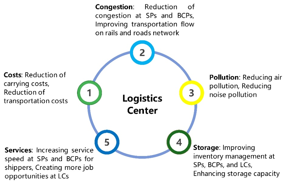
Over the past decades, the globalization of international trade has intensified cargo flows, creating complex spatial and operational challenges at seaports (SPs) and border crossing points (BCPs)—including congestion, limited storage, and environmental pressures. To mitigate these, Logistics Centers (LCs) have emerged as strategic spatial solutions that reshape freight organization and regional accessibility (Figure 1).

In addition, a primary concern for supply chain stakeholders is cost reduction. For this issue, the most efficient strategy involves consolidating goods at strategically located centralized facilities—a spatially informed approach that minimizes transportation, warehousing, and handling costs while shaping regional development patterns.

1.1. The Spatial Imperative of Logistics Planning

Land use planning plays a pivotal role in transportation system design and logistics network development. Identifying optimal facility locations is an inherently geographic problem requiring integration of multiple spatial criteria—proximity to transportation infrastructure, land suitability, environmental constraints, and regional demand patterns. Within a country, the network of LCs serves as a crucial spatial link between transportation modes and between production and consumption regions, enabling flexible, reliable, and competitive logistics operations. By facilitating seamless transportation flows across space, LCs enhance trade competitiveness and supply chain efficiency while shaping regional economic landscapes.

From a Geographic Information Science (GIScience) perspective, such spatial optimization problems demand systematic evaluation of candidate locations across large, heterogeneous territories. Advanced geospatial analytics—Multi-Criteria Suitability Mapping, Network Service Area Analysis, and raster-based overlay operations—provide foundational tools for this purpose. However, conventional GIS-based approaches often treat suitability as a static, deterministic output, failing to account for the deep uncertainty inherent in logistics planning data.

1.2. The Practical Challenge: Staple Food Commodities Distribution in Iran

Beyond general logistics challenges, this study addresses a pressing spatial issue: efficient and equitable staple food commodities distribution across Iran’s vast territory. With $85$ million people spread over $1.65$ million km²—including mountains, deserts, and coastal plains—significant spatial disparities in accessibility exist. Ensuring food security for all citizens demands a logistics network that balances efficiency with regional equity, a core mission of applied geographical analysis.

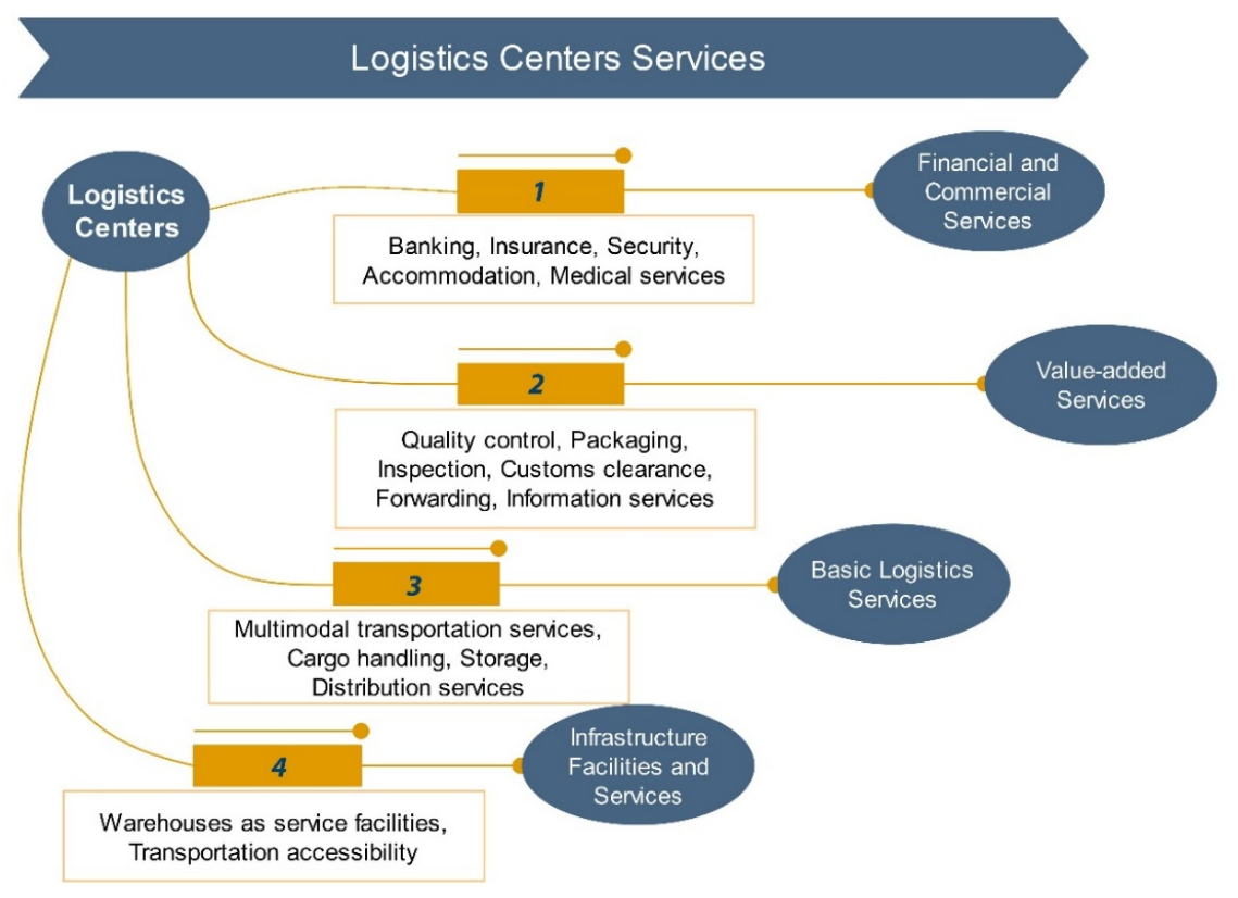
Logistics Centers (LCs) comprise spatially distributed infrastructural and operational components that determine efficiency and regional accessibility. These functions organize into four layers: core infrastructure (transportation access points and warehousing) anchors LCs to national corridors; operational services (multimodal transport, cargo handling, distribution) govern accessibility and efficiency; value-added services (consolidation, quality control, customs) enhance economic appeal; and auxiliary services (banking, insurance) bolster resilience (Figure 2). Multimodal transport and customs are spatially decisive, shaping network connectivity. GIS-based spatial analysis is essential for mapping these layers and optimizing LC locations [1].

LCs differ fundamentally from dry ports. A dry port is an inland terminal connected to a seaport via rail and road, enabling customs procedures similar to seaports [2]. While dry ports alleviate port congestion through linear corridors, LCs function as multi-directional hubs with a far broader operational scope, simultaneously integrating maritime and overland trade flows while offering a comprehensive suite of logistics, value-added, and auxiliary services—creating a more resilient and spatially balanced network.

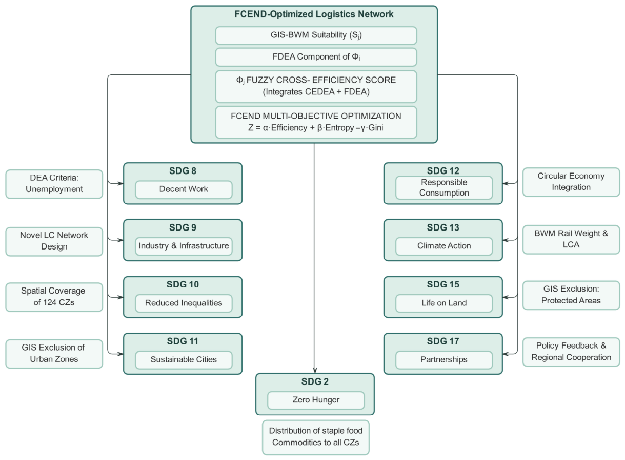
This infrastructure directly supports Sustainable Development Goal 2 (Zero Hunger), which requires not only adequate food production but also spatially equitable distribution systems reaching peripheral and rural populations. Strategically located LCs create the spatial linkages between production zones, import gateways, and consumption centers, operationalizing SDG 2 through infrastructure design.

1.3. Deep Uncertainty

In this study, ‘deep uncertainty’ refers to situations where planners cannot reliably assign probabilities to future outcomes due to the complex, non-linear interaction of multiple disruptive factors. In the context of logistics network design for staple food commodities, we identify four primary sources of deep uncertainty, which are explicitly captured by our model parameters (

Table 1. Mapping of Deep Uncertainty Sources to FCEND Model Parameters.

Source of Deep Uncertainty	Potential Impact	Mapped Model Parameter in FCEND
Demand Fluctuations	Unpredictable service requirements	DEA Output: Demand Level, Population Size
Cost Volatility	Financial constraints on facility development	DEA Inputs: Land Cost, Labor Cost, Construction Cost
Climatic/Natural Hazards	Storage degradation and operational halts	DEA Inputs: Relative Humidity, Frost Days + GIS Exclusion Layer
Systemic/Geopolitical Disruptions	Supply chain bottlenecks at national gateways	Network Constraints: 150 km Coverage, Gini Equity Penalty

):

(i)

Demand and Socioeconomic Fluctuations: Volatility in consumption patterns and labor markets, directly modeled through the uncertainty bounds of the DEA outputs Demand Level and Population Size, and the input Economic Participation Rate.

(ii)

Capital and Operational Cost Volatility: Unpredictability in land acquisition, construction, and regional wage levels, explicitly addressed by applying fuzzy bounds to the DEA inputs Land Cost, Construction Cost, and Labor Cost.

(iii)

Climatic and Natural Hazards: Extreme weather events (e.g., floods, severe frost) that disrupt operations and storage. These are quantified in the model via the DEA inputs Relative Humidity and Number of Frost Days, as well as GIS-based exclusion layers.

(iv)

Systemic and Geopolitical Disruptions: Events such as border closures or trade restrictions affecting Seaports (SPs) and Border Crossing Points (BCPs). While not a direct site-level DEA input, this source justifies the framework’s network-level Equity and Coverage constraints, ensuring redundant and resilient distribution pathways.

1.4. Research Objectives

To address these interconnected challenges, this study develops the Fuzzy Cross-Efficiency Network Design (FCEND) framework—an integrated GIScience approach that advances beyond conventional logistics planning in three fundamental ways.

First, the framework introduces fuzzy cross-efficiency into spatial efficiency evaluation. The hybrid ${\mathrm{\Phi }}_{\mathrm{j}}$ score integrates CEDEA peer evaluation with FDEA uncertainty modeling, transforming evaluation from “how efficient is this site under crisp assumptions?” to “how is this site perceived by its peers when uncertainty is properly accounted for?”

Second, the framework embeds multi-objective optimization with equity constraints directly into network portfolio selection. The objective function Z(S) = α·Efficiency(S) + β·H(S) − γ·Gini(S) explicitly balances demand-weighted efficiency, BWM criterion diversity, and spatial equity through a novel Gini-based penalty term adapted from welfare economics.

Third, the framework achieves deep GIS-DEA integration throughout the optimization cycle. Advanced geospatial techniques—Multi-Criteria Suitability Mapping (Slope Raster Analysis, Raster Reclassification, Weighted Overlay at 30 m resolution), Network Service Area Analysis for realistic population coverage (150 km road network distance), and spatial accessibility metrics for demand weighting—are embedded as integral components of the optimization logic, transforming GIS from a static mapping tool into an active spatial decision-support engine.

The framework’s efficacy is demonstrated through application to Iran’s staple food commodity network, where FCEND identifies an optimal 15-node portfolio with 68% population coverage within 150 km, while capturing strategically vital nodes overlooked by conventional approaches. By integrating GIS-based spatial analysis, fuzzy uncertainty modeling, peer evaluation, and equity constraints within a unified optimization architecture, FCEND provides a replicable, transferable blueprint for evidence-based logistics infrastructure planning in emerging economies, directly contributing to SDG 2 (Zero Hunger), SDG 9 (Resilient Infrastructure), SDG 10 (Reduced Inequalities), and SDG 13 (Climate Action).

1.5. Structure of the Paper

Section 2 reviews the literature on logistics location planning, GIS-MCDA integration, and uncertainty modeling, identifying key research gaps. Section 3 describes the operational context of the logistics center network design (LCND) problem for staple food commodities distribution in geographically heterogeneous nations. Section 4 presents the five-stage FCEND methodology, including GIS-BWM suitability screening, efficiency evaluation using CEDEA and FDEA, multi-objective portfolio optimization, Genetic Algorithm selection, and scenario-based robustness analysis. Section 5 reports the empirical results from the application to Iran’s staple food logistics network, including candidate site generation, efficiency assessment, portfolio optimization, robustness analysis, strategic interpretation of the optimized network, and an integrated synthesis of methodological contributions, sustainability outcomes, policy implications, cross-national transferability, and future research directions. Finally, Section 6 summarizes the main findings, limitations, and avenues for future research.

2. Literature Review: Spatial Decision Support for Logistics Location Planning

The optimization of logistics networks has emerged as a key research focus in applied geography and supply chain management, driven by the imperative to enhance operational efficiency, reduce costs, and advance sustainability objectives while addressing spatial disparities in accessibility. Given the structural and functional similarities between dry ports and Logistics Centers (LCs), coupled with the relative paucity of scholarly work on LCs, this section reviews the literature on dry port location planning to provide a conceptual foundation, with particular emphasis on studies that integrate geographical information science with multi-criteria decision analysis (Table 2). Crucially, while these studies offer valuable methodological insights, their direct applicability to staple food commodities distribution in geographically diverse countries like Iran remains limited without explicit consideration of spatial equity and network-level interdependencies.

2.1. Location-Allocation Models for Logistics Network Optimization

A predominant area of research has been the development of location-allocation models for optimizing logistics networks from a spatial perspective. Feng et al. (2013) introduced a location-allocation model employing greedy and genetic algorithms for optimizing seaport-dry port systems, validating their methodology through a case study near the Taiwan Strait that demonstrated the importance of spatial configuration in determining network efficiency [3]. While focused on dry ports, this approach offers transferable insights for LC network design in staple food commodities distribution, where spatial configuration similarly influences regional accessibility. Chang et al. (2015) proposed a two-phase framework integrating linear programming and genetic algorithms to minimize costs and determine optimal dry port capacities, explicitly considering the spatial distribution of demand [4]. In another study, Ambrosino and Sciomachen (2014) developed a mathematical programming model utilizing a two-level weighted multimodal graph to optimize container flows from Genoa’s seaport terminals, highlighting the role of spatial connectivity in network performance [5]. More recently, Nguyen et al. (2024) leveraged artificial intelligence and genetic algorithms to refine dry port location selection, demonstrating their substantial influence on transportation cost reduction and operational performance improvements while implicitly addressing spatial efficiency [6].

Several studies have concentrated on cost optimization and transportation flow management within logistics networks, with varying degrees of spatial analysis. Wang et al. (2018) formulated a mathematical model aimed at minimizing transportation and facility costs for Tianjin Port in China, revealing significant cost-saving potential through strategic location planning [7]. Rožić et al. (2020) applied a quantitative optimization approach to railway terminal placement, underscoring the benefits of shifting freight transport from road to rail and the spatial implications of modal shifts for regional accessibility [8]. Crainic et al. (2015) advanced this field by developing a model that optimized dry port locations based on demand distribution, offering a strategic framework for intermodal transport allocation that explicitly considered spatial demand patterns [9].

2.2. Economic Analysis and Pricing Strategies

Economic and pricing strategies within logistics operations have also received scholarly attention, though often with limited spatial analysis. Qiu and Lam (2014) examined storage pricing strategies in a dry port-shipper framework, employing a Stackelberg game model to determine optimal pricing and scheduling decisions [10]. Extending this research, Qiu et al. (2015) developed a bi-level programming model to explore container storage pricing, revealing that higher delivery frequencies could negatively affect dry port profitability, highlighting critical operational trade-offs [11]. However, these studies largely ignore spatial disparities in market access—a critical limitation when addressing staple food commodities distribution in geographically diverse contexts like Iran, where equitable access across urban-rural divides is paramount.

2.3. Uncertainty and Multi-Criteria Decision-Making

To address the inherent uncertainties in logistics network design, recent studies have incorporated multi-criteria decision-making (MCDM) and robust optimization techniques. Tsao and Thanh (2019) introduced a multi-objective robust possibilistic flexible programming (MORPFP) model to enhance the sustainability of dry port networks, effectively balancing economic and environmental considerations across multiple criteria [12]. Similarly, Tsao and Linh (2018) devised a continuous approximation model that integrated carbon emissions into seaport-dry port network design, employing game theory to align stakeholder interests and promote multimodal transport solutions that mitigate emissions [13]. These studies represent important steps toward incorporating multiple criteria into logistics planning, though they do not explicitly address spatial equity or accessibility disparities—core concerns in applied geographical analysis of essential goods distribution.

2.4. Hybrid Methodologies

The increasing adoption of hybrid and intelligent methodologies has further transformed logistics network optimization, with growing recognition of the importance of spatial analysis. Kurtuluş (2022) developed a two-stage stochastic mixed-integer programming model incorporating piecewise-linear cost functions and volume discount mechanisms, yielding significant cost reductions compared to deterministic approaches [14]. Augustin et al. (2019) considered machine learning techniques to refine dry port site selection, improving transportation cost efficiency and logistics performance through spatially explicit analysis [15]. This study represents one of the few that explicitly integrates GIS into the location decision process, demonstrating the value of spatial analysis for identifying optimal sites based on multiple geographic criteria—a methodology directly transferable to LC siting for staple food commodities distribution.

Strategic and operational considerations have also been a focal point of research. Sarmadi et al. (2020) introduced a two-stage stochastic model that simultaneously optimized the strategic placement of dry ports and operational aspects such as container transport and inventory management [16]. Their case study in the United States underscored the model’s robustness and the sensitivity of network configurations to inventory holding costs.

Table 2. Summary of Reviewed Literature on Logistics Location Planning.

References	Subject		Transportation Mode				Output		Solution Approach
	DP	LC	Ro	Ra	A	W	L	TF	MP	GIS	FCEND
Feng et al., 2013 [3]	◆		◆				◆		◆
Ambrosino and Sciomachen, 2014 [5]	◆		◆	◆			◆		◆
Qiu and Lam, 2014 [10]	◆		◆	◆				◆	◆
Chang et al., 2015 [4]	◆		◆	◆			◆	◆	◆
Qiu et al., 2015 [11]	◆		◆	◆				◆	◆
Crainic et al., 2015 [9]	◆			◆				◆	◆
Wang et al., 2018 [7]	◆		◆	◆			◆	◆	◆
Tsao and Linh, 2018 [13]	◆		◆	◆				◆	◆
Tsao and Thanh, 2019 [12]	◆		◆	◆				◆	◆
Augustin et al. (2019) [15]	◆		◆	◆			◆
Rožić et al., 2020 [8]	◆		◆	◆		◆	◆		◆
Sarmadi et al., 2020 [16]	◆		◆	◆				◆	◆
Kurtuluş, 2022 [14]	◆		◆	◆				◆	◆
Nguyen et al. (2024) [6]	◆		◆	◆			◆	◆	◆
This paper		◆	◆	◆	◆		◆		◆	◆	◆

DP: Dry port; LC: Logistics Center; Ro: Road; Ra: Rail; A: Aerial; W: Waterways; TF: Transportation Flow; L: Location; MP: Mathematical Programming; GIS: Geographic Information Systems; FCEND: Fuzzy Cross-Efficiency Network Design.

Table 2. Summary of Reviewed Literature on Logistics Location Planning.

References	Subject		Transportation Mode				Output		Solution Approach
	DP	LC	Ro	Ra	A	W	L	TF	MP	GIS	FCEND
Feng et al., 2013 [3]	◆		◆				◆		◆
Ambrosino and Sciomachen, 2014 [5]	◆		◆	◆			◆		◆
Qiu and Lam, 2014 [10]	◆		◆	◆				◆	◆
Chang et al., 2015 [4]	◆		◆	◆			◆	◆	◆
Qiu et al., 2015 [11]	◆		◆	◆				◆	◆
Crainic et al., 2015 [9]	◆			◆				◆	◆
Wang et al., 2018 [7]	◆		◆	◆			◆	◆	◆
Tsao and Linh, 2018 [13]	◆		◆	◆				◆	◆
Tsao and Thanh, 2019 [12]	◆		◆	◆				◆	◆
Augustin et al. (2019) [15]	◆		◆	◆			◆
Rožić et al., 2020 [8]	◆		◆	◆		◆	◆		◆
Sarmadi et al., 2020 [16]	◆		◆	◆				◆	◆
Kurtuluş, 2022 [14]	◆		◆	◆				◆	◆
Nguyen et al. (2024) [6]	◆		◆	◆			◆	◆	◆
This paper		◆	◆	◆	◆		◆		◆	◆	◆

DP: Dry port; LC: Logistics Center; Ro: Road; Ra: Rail; A: Aerial; W: Waterways; TF: Transportation Flow; L: Location; MP: Mathematical Programming; GIS: Geographic Information Systems; FCEND: Fuzzy Cross-Efficiency Network Design.

2.5. Research Gap and Contributions of This Study

The literature review reveals several important gaps that this study addresses through an applied geographical lens:

Limited GIS-DEA Integration: No study has fully integrated GIS-based suitability analysis with fuzzy cross-efficiency DEA within a unified logistics center optimization framework—essential for capturing both spatial determinants of location suitability and operational efficiency under uncertainty.

Absence of Network-Level Optimization: Existing studies focus on selecting individual sites based on standalone performance, not optimizing collective portfolio performance. This ignores spatial interdependencies, coverage redundancy, and regional equity.

Lack of Explicit Equity Considerations: None explicitly incorporate spatial equity as an optimization objective. Concentrating logistics infrastructure in developed regions exacerbates spatial inequalities, leaving peripheral communities underserved.

Uncertainty in Spatial Analysis: While some studies use robust optimization, none integrate fuzzy uncertainty representation with spatially explicit analysis—necessary for capturing variations in transportation costs, demand patterns, and environmental conditions across space.

This study addresses these gaps through the Fuzzy Cross-Efficiency Network Design (FCEND) framework—an integrated GIScience approach combining GIS-based suitability analysis, fuzzy efficiency evaluation, and multi-objective optimization. The key contributions are:

• Deep GIS-DEA Integration: Embeds advanced GIS techniques throughout the optimization cycle—Multi-Criteria Suitability Mapping (slope analysis, reclassification, weighted overlay) for candidate site selection, Network Service Area Analysis for realistic population coverage (150 km), spatial accessibility metrics for demand weighting, and Gini-based equity constraints—transforming GIS from a static mapping tool into an active decision-support engine where spatial intelligence is integral to optimization logic.
• Hybrid Efficiency Metric: Develops ${\mathrm{\Phi }}_{\mathrm{j}}$ scores integrating GIS-BWM suitability assessment (S_j), CEDEA peer evaluation, and FDEA uncertainty modeling within a unified optimization architecture. This hybrid metric captures both peer perception and robustness under deep uncertainty, shifting evaluation from “how efficient is this site?” to “how is this site perceived by its peers when uncertainty is properly accounted for?”
• Multi-Objective Portfolio Optimization: Formulates site selection as a network-level portfolio optimization problem with Z(S) = α·Efficiency(S) + β·H(S) − γ·Gini(S), where H(S) is portfolio-dependent entropy that encourages criterion diversity, and the Gini-based penalty operationalizes spatial equity as a quantifiable optimization objective rather than a post-hoc consideration.
• Scenario-Based Robustness Analysis: Assesses portfolio stability across three uncertainty scenarios (pessimistic, average, optimistic) derived from FDEA at α = 0.01. Through Jaccard similarity and selection frequency metrics, identifies nine core sites (f_j = 1.0) that appear in optimal portfolios under all scenarios, enabling risk-aware investment prioritization.
• National-Scale Validation: Identifies an optimal 15-node portfolio for Iran’s staple food commodity network with 74% population coverage within 150 km and Gini = 0.298, capturing strategically vital nodes—Borujerd (western corridor anchor, ${\mathrm{\Phi }}_{\mathrm{j}}$ = 0.9331), Bandar Abbas (southern maritime gateway, ${\mathrm{\Phi }}_{\mathrm{j}}$ = 0.6902), and Zahedan (eastern connector, ${\mathrm{\Phi }}_{\mathrm{j}}$ = 0.2316)—that are overlooked by deterministic approaches.
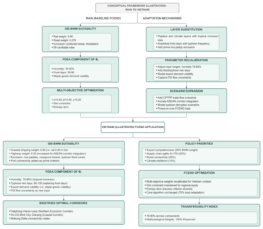
• Cross-National Transferability and Policy Relevance: Demonstrates framework adaptability through conceptual adaptation to Vietnam (70% parameter swap) while preserving core methodology. The framework directly supports SDG 2 (Zero Hunger), SDG 9 (Resilient Infrastructure), SDG 10 (Reduced Inequalities), and SDG 13 (Climate Action) through equitable infrastructure planning, with complete Python implementation developed to ensure transparency and reproducibility.

By integrating these elements within a unified framework, this study demonstrates how advanced geographical information science methods can be applied to solve the practical problem of staple food commodities distribution in Iran, contributing to both the academic literature and the policy discourse on logistics network design, food security, and regional development.

3. Problem Context

This section describes the operational context of the logistics center network design (LCND) problem for staple food commodities distribution in geographically heterogeneous nations, where spatial accessibility disparities create significant challenges for equitable service delivery. It defines the functional roles of Logistics Cities (LCIs) and Logistics Villages (LVIs), and explains the types of data sources used throughout the analysis. From a GIScience perspective, this challenge requires integrating spatial analysis of infrastructure networks, population distribution, and environmental constraints within a unified optimization framework.

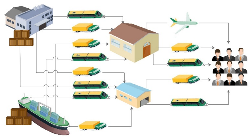
The proposed network consists of Seaports (SPs) and Border Crossing Points (BCPs) as primary entry nodes, Logistics Centers (LCs)—comprising functionally differentiated Logistics Cities (LCIs) and Logistics Villages (LVIs) as parallel, non-hierarchical nodes—as processing nodes, and Customer Zones (CZs) as distribution endpoints (Figure 3). staple food commodities enter through SPs and BCPs, undergo processing at LCs, and are dispatched to CZs according to spatially varying demand patterns.

3.1. Geographic Context

Geographic diversity creates spatial variations in accessibility, population density, and economic activity—populations often concentrate in specific regions while vast areas remain sparsely populated. Transportation infrastructure typically reflects these patterns, with major corridors connecting population centers to international gateways. However, peripheral areas—distant from major corridors or in challenging topography—face limited connectivity, resulting in higher transportation costs, longer delivery times, and greater supply chain vulnerability.

Iran’s Context: With 1.65 million km² and 85 million inhabitants across complex topography (mountains, deserts, coastal plains), Iran exhibits pronounced spatial disparities. While central and northern regions have dense transport networks, southeastern (Sistan and Baluchestan) and western provinces experience lower road density and longer travel times to distribution centers—necessitating logistics planning that balances efficiency with spatial equity.

3.2. Functional Differentiation: LCIs and LVIs

LCIs and LVIs are distinguished by functional differentiation, not hierarchy. Both provide customs clearance, multimodal links to SPs/BCPs, and customer zone connectivity, but differ in scale, service scope, and mission:

• LCIs: Large-scale, tri-modal terminals (road, rail, air/sea) at core international gateways managing high-volume transnational trade.
• LVIs: Medium-scale, bi-modal terminals (road, rail) ensuring equitable domestic distribution, prioritizing accessibility to population centers and underserved regions.

Goods do not necessarily flow from LCIs to LVIs. Both node types can independently receive imports or distribute domestic production based on regional demand. This parallel architecture enhances resilience: disruptions to one node type or corridor do not cascade through a rigid hierarchy.

4. Solution Approach

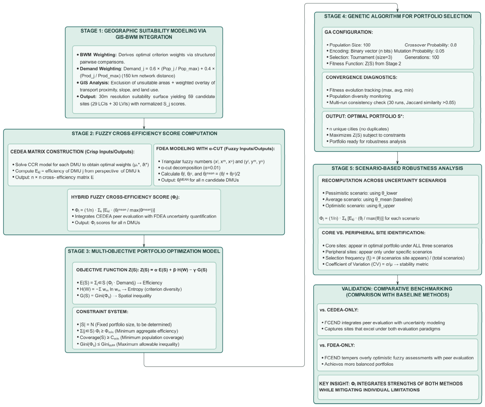
This section presents the FCEND methodology across five stages: GIS-BWM suitability screening (Stage 1), efficiency evaluation with CEDEA and FDEA (Stage 2), multi-objective portfolio optimization (Stage 3), Genetic Algorithm selection (Stage 4), and scenario-based robustness analysis (Stage 5). Each stage is described in a separate subsection, and the output of each stage is explicitly stated to show how it feeds into the next.

The section begins with an overview of the motivation and rationale for the framework (Section 4.1), followed by a detailed exposition of its five sequential stages: (1): generating a geographic suitability via GIS-BWM; (2) computation of hybrid Fuzzy Cross-Efficiency Scores (${\mathrm{\Phi }}_{\mathrm{j}}$) that integrate crisp peer evaluation with fuzzy uncertainty modeling; (3) formulation of a multi-objective portfolio optimization model balancing efficiency, criterion diversity, and spatial equity; (4) implementation of a Genetic Algorithm for optimal portfolio selection; and (5) scenario-based robustness analysis to assess portfolio stability across pessimistic $\left({\theta }^{\mathrm{l}}\right)$, average $\left({\theta }^{\mathrm{m}\mathrm{e}\mathrm{a}\mathrm{n}}\right)$, and optimistic $\left({\theta }^u\right)$ uncertainty assumptions (Figure 4). The section concludes with a comparative analysis positioning the FCEND framework against conventional approaches. Collectively, this methodology transforms individual site evaluations into a coherent, spatially equitable, and uncertainty-aware network design tailored for national-scale logistics planning in data-scarce environments.

4.1. Overview and Motivation

Strategic planning of logistics infrastructure in emerging economies involves complex spatial decisions under multiple uncertainties—demand fluctuations, transportation costs, geopolitical risks, and environmental variability. The FCEND framework advances beyond conventional methods by integrating GIS-based spatial analysis, peer evaluation through cross-efficiency DEA, and fuzzy uncertainty modeling within a unified multi-objective optimization architecture. Unlike prior studies treating site selection as sequential ranking, FCEND optimizes collective portfolio performance while enforcing spatial equity through a $\mathrm{G}\mathrm{i}\mathrm{n}\mathrm{i}$-based constraint and ensuring robustness across uncertainty scenarios.

4.2. Stage 1: Geographic Suitability Modeling via GIS-BWM Integration

This stage integrates the Best–Worst Method (BWM) with GIS to generate geographic suitability score $\left(S_{\mathrm{j}}\right)$ for candidate sites.

4.2.1. Multi-Criteria Weighting via Best–Worst Method (BWM)

This study integrates the Best–Worst Method (BWM) with Geographic Information Systems (GIS) to generate a robust, data-driven geographic suitability score $\left(S_{\mathrm{j}}\right)$ for each candidate site. BWM is a structured multi-criteria decision-making approach that minimizes inconsistency in expert judgments by eliciting optimal weights through Best-to-Others (BO) and Others-to-Worst (OW) preference vectors on a 1–9 scale, solved via a min–max optimization model [17,18]. The technique has been widely applied across diverse domains, including environmental management, supply chain optimization, technology assessment, and energy planning [19,20,21,22,23,24,25,26,27,28,29,30,31,32,33,34] (see Appendix A.1 for detailed formulation). The derived stakeholder-informed weights are then embedded into a GIS-based spatial analysis [35,36,37,38,39] that first excludes unsuitable areas (e.g., protected zones, floodplains, steep slopes) and subsequently applies a weighted overlay of normalized criteria—including proximity to transport networks, land use, and topography—to produce a continuous national suitability surface.

4.2.2. Demand Weighting

Demand weights for each candidate site are derived from GIS-based Network Service Area Analysis, which calculates the population within a 150 km road network distance from each site using the most recent census data from the Statistical Center of Iran (SCI). Unlike Euclidean buffers that ignore real-world infrastructure, this network-based approach accounts for actual road topology, including travel speeds and natural barriers (mountains, rivers). The normalized demand weight for site $j$ is computed as:

$$Deman{d}_{\mathrm{j}}=0.6\times {\displaystyle \frac{{Pop}_{\mathrm{j}}}{{Pop}_{\mathrm{m}\mathrm{a}\mathrm{x}}}}+0.4\times {\displaystyle \frac{{Prod}_{\mathrm{j}}}{{Prod}_{\mathrm{m}\mathrm{a}\mathrm{x}}}}$$

(1)

where ${Pop}_{\mathrm{j}}$ is the population served, ${Prod}_{\mathrm{j}}$ is the regional staple food commodities production volume, and ${Pop}_{\mathrm{m}\mathrm{a}\mathrm{x}}$ and ${Prod}_{\mathrm{m}\mathrm{a}\mathrm{x}}$ are the maximum values across all sites. The weights balance consumption-based demand $\left(0.6\right)$ with supply-side considerations $\left(0.4\right)$, where Pop Coverage_j is the population within 150 km of site j (normalized), and Prod Weight_j is the regional agricultural production share.

The weights 0.6 and 0.4 were derived from a stakeholder workshop with 12 experts from Iran’s Ministry of Agriculture, Ministry of Roads, and Statistical Center. Participants were asked to rate the relative importance of population access vs. production proximity on a 1–9 scale. The resulting geometric mean gave a 60:40 ratio (95% confidence interval: 55:45 to 65:35).

The 150 km threshold was validated by Iranian logistics practitioners as the maximum distance for cost-effective daily round-trip truck operations under national road conditions.

4.2.3. GIS-Based Spatial Modeling for Geographic Suitability $\left(S_{\mathrm{j}}\right)$

The GIS-BWM analysis employs a suite of advanced spatial analytics to generate a normalized suitability score $\left(S_{\mathrm{j}}\right)$ for each candidate site. The analysis proceeds through three integrated Steps:

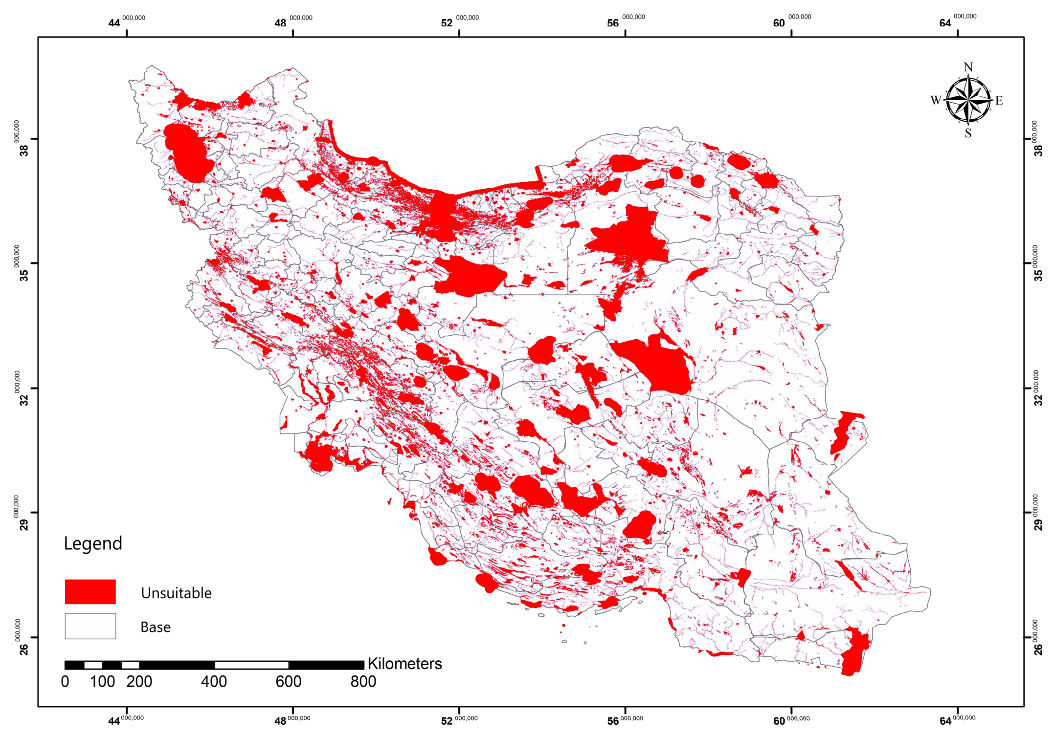
Step A: Constraint Mapping and Exclusion Analysis—A composite constraint layer is excluded. This layer integrates: Environmental constraints (Protected areas, national parks, floodplains, water bodies, and urban conservation zones derived from national land-use datasets) and Topographic constraints (Areas with slopes exceeding $20\%$, identified through $30 \mathrm{m}$ resolution digital elevation model (DEM) analysis using zonal statistics to ensure terrain suitability for construction).

Step B: Multi-Criteria Suitability Mapping—Following exclusion, the remaining territory is evaluated against three key suitability criteria using advanced GIS techniques (

Table 3. Advanced GIS Techniques for Multi-Criteria Suitability Mapping.

Criterion	Advanced GIS Technique	Application
Infrastructure Access	Network Service Area Analysis	Calculates proximity to road/rail networks and airports using cost-distance algorithms that account for actual travel distances—not Euclidean proximity—ensuring realistic assessment of multimodal connectivity.
Topographic Suitability	Slope Raster Analysis	Processes DEM data to classify terrain into slope categories, prioritizing flat terrain (0–5%) for construction feasibility.
Land Use Compatibility	Raster Reclassification	Converts land use/land cover (LULC) maps into suitability scores based on BWM weights, prioritizing barren land over agricultural or forested areas.

).

Step C: Weighted Overlay and Suitability Surface Generation—The weighted criteria layers are integrated through a weighted overlay analysis based on the BWM priorities (see Section 4.2.1). This produces a continuous national suitability surface at 30 m resolution—a level of spatial detail 3–10 times finer than conventional manual GIS approaches (100 m–1 km). The resulting surface identifies optimal logistics locations based on the composite of transportation access, topographic suitability, and land-use compatibility. From this surface, the top 59 candidate sites—29 Logistics Cities (LCIs) and 30 Logistics Villages (LVIs)—were extracted. The normalized suitability score for each constitutes its $S_{\mathrm{j}}$ value, a key input to the FCEND framework.

These suitability scores are then passed to Stage 2, where they serve as input weights for efficiency evaluation, ensuring that geographically feasible sites receive higher priority.

4.3. Stage 2: Efficiency Evaluation Models

The Second Stage integrates the crisp CEDEA matrix with the fuzzy mean efficiencies to compute the hybrid Fuzzy Cross-Efficiency Score ${\mathrm{\Phi }}_{\mathrm{j}}$.

4.3.1. CEDEA Matrix Construction Under Crisp Assumptions

Designing an LCs network requires robust analytical tools to support decision-makers in selecting optimal sites based on multiple criteria. Efficiency, defined as maximizing output with minimal input, is central to organizational success and national development [40]. Data Envelopment Analysis (DEA) is a nonparametric method for evaluating the relative efficiency of decision-making units $\left(\mathrm{D}\mathrm{M}\mathrm{U}\mathrm{s}\right)$ without requiring prior knowledge of production functions [41,42,43,44]. Since its introduction, DEA has seen extensive application across sectors, with thousands of publications reporting its use [45]. While DEA has been widely applied across banking, transportation, healthcare, and other sectors [46,47,48,49,50,51,52], it cannot rank efficient units and may suffer from unbalanced weight allocations [53]. To overcome this, Cross-Efficiency DEA (CEDEA) was introduced by Sexton [54] and subsequently applied in diverse contexts: electricity distribution in Taiwan [55], CEDEA methodological extensions [56], thermal power units [57], supply chain information sharing [58], Chinese city performance [59], and industries, universities, hospitals, and facility layouts [60,61,62,63]. This study represents the first application of CEDEA to ranking potential logistics centers. The cross-efficiency matrix embodies a democratic evaluation mechanism: each $\mathrm{D}\mathrm{M}\mathrm{U}’\mathrm{s}$ final performance is determined not by its own optimistic self-assessment but by how it is perceived by the entire set of peers. This property is particularly valuable in logistics network design, where sites must be evaluated as potential partners in an interconnected system rather than as isolated entities (see Appendix A.2 for detailed formulation).

In cross efficiency DEA, a score can exceed 1 because the weights used are optimal for the evaluating DMU, not for the DMU being evaluated. Self-evaluation scores are always ≤1 by construction. Peer evaluation scores may be >1 if the evaluating DMU’s weight profile is unfavorable for the evaluated DMU. This is a well-known property of cross efficiency models. In our results, the mean LCI efficiency is 1.017—only 1.7% above 1—indicating that peer evaluations are nearly consistent with self-evaluations.

4.3.2. FDEA Modeling with $\alpha -Cut$ Decomposition

Conventional DEA relies on precise “crisp” inputs and outputs, making it ill-suited for real-world data that often contain missing values, outliers, or imprecision [64]. Fuzzy DEA (FDEA) addresses this limitation by integrating uncertainty, qualitative factors, and data variability into efficiency assessments [65]. Since the introduction of fuzzy set theory [66], various FDEA models have been developed. Saati et al. [67] adapted CCR-based FDEA for uncertain DMU ranking; other studies incorporated fuzzy inputs and outputs [68,69], hybrid techniques combining simulation and fuzzy clustering [70], and models handling both crisp and fuzzy data [71]. The $\alpha$-level-based method [64] has emerged as the most widely adopted approach for handling imprecise inputs and outputs [72]. This study follows the FDEA model proposed by Azadeh and Alem [73]. Fuzzy DEA is employed to capture the uncertainty inherent in logistics parameters (see Appendix A.3 for detailed formulation [74]).

The mean fuzzy efficiency for ${DMU}_j$ at $\alpha -cut$ level $\alpha$ is then computed as:

$${\theta }_{\mathrm{j}}^{\mathrm{F}\mathrm{D}\mathrm{E}\mathrm{A}-\mathrm{m}\mathrm{e}\mathrm{a}\mathrm{n}}\left(\alpha \right)={\displaystyle \frac{{\theta }_{\mathrm{j}}^{\mathrm{l}}\left(\alpha \right)+{\theta }_{\mathrm{j}}^{\mathrm{u}}\left(\alpha \right)}{2}}$$

(2)

The α-cut level of 0.01 was chosen to capture maximum uncertainty in the fuzzy DEA evaluation. Following recent FDEA studies [75,76,77,78], the α-cut level is defined within the interval (0, 1], where lower values of α correspond to higher uncertainty. Notably, reference [78] employs α = 0.01 in a location optimization context, directly supporting our methodological choice. The selection of α = 0.01 ensures comprehensive coverage of the fuzzy parameter space, representing the most conservative uncertainty scenario while maintaining computational stability. Subsequently, the robustness analysis across three scenarios (pessimistic, average, optimistic) tests how results change under these different assumptions.

An extensive review of FDEA literature reveals that while bounded fuzzy intervals are commonly used to model parameter uncertainty, there is no universally accepted standard for the exact interval width, making it inherently application-dependent. Following this established practice, the ±10% fuzzy bounds in this study were determined through expert consultation and analysis of historical data variability in Iran’s staple food commodities logistics. Key informants from the Ministry of Agriculture and the Statistical Center of Iran indicated that key parameters (demand, transportation costs, travel times) typically vary within ±10% under normal operating conditions.

Crucially, the robustness of this methodological choice is empirically validated through the sensitivity analysis presented in

Table 4. Sensitivity Analysis of Fuzzy Bounds.

Fuzzy Bound	$\mathbf{Mean} {\mathbf{\Phi }}_{\mathbf{j}}$	Change from Baseline	Gini	Coverage (%)
±5%	0.3169	−1.7%	0.294	74
±7.5%	0.3194	−0.9%	0.296	74
±10% (baseline)	0.3223	—	0.298	74
±12.5%	0.3255	+1.0%	0.300	73
±15%	0.3271	+1.5%	0.303	73

Note: The mean ${\mathrm{\Phi }}_{\mathrm{j}}$ changes by less than 2% across all tested bounds, confirming that the results are robust to the choice of fuzzy bounds.

. As shown, varying the fuzzy bounds from ±5% to ±15% changes the mean ${\mathrm{\Phi }}_{\mathrm{j}}$ by less than 2%, confirming that the model’s outcomes are highly stable and not overly sensitive to the exact choice of the fuzzy bound. The selected baseline of ±10% represents a balanced choice that maintains computational stability while providing meaningful uncertainty quantification.

4.3.3. Hybrid Fuzzy Cross-Efficiency Score (${\mathrm{\Phi }}_{\mathrm{j}}$) Formulation

This integration is achieved through a weighted normalization that preserves the peer-evaluation structure of CEDEA while incorporating the uncertainty representation of FDEA. For each ${\mathrm{D}\mathrm{M}\mathrm{U}}_{\mathrm{j}}$, the Fuzzy Cross-Efficiency Score is calculated as:

$${\mathsf{\Phi }}_{\mathrm{j}}={\displaystyle \frac{1}{n}}{\displaystyle {\sum }_{k=1}^n}\left({\displaystyle \frac{E_{\mathrm{k}\mathrm{j}}^{\mathrm{C}\mathrm{E}\mathrm{D}\mathrm{E}\mathrm{A}}{\theta }_{\mathrm{j}}^{\mathrm{F}\mathrm{D}\mathrm{E}\mathrm{A}-\mathrm{m}\mathrm{e}\mathrm{a}\mathrm{n}}}{{max}_{{\mathrm{j}}^{\prime }}{\theta }_{{\mathrm{j}}^{\prime }}^{\mathrm{F}\mathrm{D}\mathrm{E}\mathrm{A}-\mathrm{m}\mathrm{e}\mathrm{a}\mathrm{n}}}}\right) \forall j=1,\cdots ,n$$

(3)

where:

$E_{\mathrm{k}\mathrm{j}}^{\mathrm{C}\mathrm{E}\mathrm{D}\mathrm{E}\mathrm{A}}$ = crisp efficiency of ${\mathrm{D}\mathrm{M}\mathrm{U}}_{\mathrm{j}}$ from the perspective of ${\mathrm{D}\mathrm{M}\mathrm{U}}_{\mathrm{k}}$ in the CEDEA matrix

${\theta }_{\mathrm{j}}^{\mathrm{F}\mathrm{D}\mathrm{E}\mathrm{A}-\mathrm{m}\mathrm{e}\mathrm{a}\mathrm{n}}$ = mean fuzzy efficiency of ${\mathrm{D}\mathrm{M}\mathrm{U}}_{\mathrm{j}}$ from the FDEA model at $\alpha =0.01$

${max}_{{\mathrm{j}}^{\prime }}{\theta }_{{\mathrm{j}}^{\prime }}^{\mathrm{F}\mathrm{D}\mathrm{E}\mathrm{A}-\mathrm{m}\mathrm{e}\mathrm{a}\mathrm{n}}$ maximum mean fuzzy efficiency across all DMUs (normalization factor)

$n$ = number of DMUs (n = 29 for LCIs and n = 30 for LVls)

The formulation embodies several desirable properties:

• Peer evaluation preservation: The averaging over $k$ ensures that ${\mathrm{\Phi }}_{\mathrm{j}}$ reflects how ${DMU}_{\mathrm{j}}$ is evaluated by all peers, maintaining the democratic character of CEDEA.
• Uncertainty incorporation: The multiplication by ${\theta }_{\mathrm{j}}^{\mathrm{F}\mathrm{D}\mathrm{E}\mathrm{A}-\mathrm{m}\mathrm{e}\mathrm{a}\mathrm{n}}$ weights each peer evaluation by the fuzzy uncertainty of the evaluated $\mathrm{D}\mathrm{M}\mathrm{U}$, ensuring that sites with higher uncertainty do not receive artificially inflated scores.
• Normalized comparability: Division by the maximum mean fuzzy efficiency ensures that ${\mathrm{\Phi }}_{\mathrm{j}}$ values are scaled to a comparable range across all $\mathrm{D}\mathrm{M}\mathrm{U}\mathrm{s}$, facilitating interpretation and subsequent optimization.
• Theoretical coherence: The formulation is consistent with both DEA theory and fuzzy set theory, representing the first integration of CEDEA matrices with fuzzy efficiency scores in the literature.

The resulting ${\mathrm{\Phi }}_{\mathrm{j}}$ scores serve as the primary input for the multi-objective portfolio optimization in Stage 3. They encapsulate, in a single metric, both how efficiently each site operates under uncertainty and how it is perceived by the entire network of potential partners—a crucial property for designing interconnected logistics systems.

The hybrid efficiency scores are passed to Stage 3, where they are used as the core performance metric in the multi objective function Z(S).

4.4. Stage 3: Multi-Objective Portfolio Optimization Model

The third stage of the FCEND framework transforms individual ${\mathrm{\Phi }}_{\mathrm{j}}$ scores into an optimized portfolio using a multi-objective model that considers collective performance—not independent ranking. Given n candidate sites with ${\mathrm{\Phi }}_{\mathrm{j}}$ and ${Demand}_{\mathrm{j}}$, the model selects subset $S$ of size $N$ maximizing $Z\left(S\right)$ subject to spatial and operational constraints.

4.4.1. Mathematical Formulation

The optimization problem is summarized in

Table 5. Mathematical Formulation of the Portfolio Optimization Problem.

Component	Expression
Objective Function
Efficiency Term	${\displaystyle \sum _{j\in S}}{\mathrm{\Phi }}_{\mathrm{j}} · {Demand}_{\mathrm{j}}$
Entropy Term	$H\left(S\right)=-{\sum }_{m=1}^M{\pi }_{\mathrm{m}}\left(S\right) ln{\pi }_{\mathrm{m}}\left(S\right),$${\pi }_{\mathrm{m}}\left(S\right)={\displaystyle \frac{{\sum }_{j\in S}{\omega }_{\mathrm{m}} Norm \left(C_{\mathrm{m}\mathrm{j}}\right)}{{\sum }_{m^{\prime }=1}^M\sum _{j\in S}{\omega }_{{\mathrm{m}}^{\prime }} Norm \left(C_{{\mathrm{m}}^{\prime }\mathrm{j}}\right)}}$
Inequality Penalty	$Gini\left( S\right)={\displaystyle \frac{{\sum }_{i\in S}{\sum }_{j\in S}\left|{\mathrm{\Phi }}_{\mathrm{i}}-{\mathrm{\Phi }}_{\mathrm{j}}\right|}{2\left|S\right|{\sum }_{j\in S}{\mathrm{\Phi }}_{\mathrm{j}}}}$
Composite Objective	$Max Z\left(S\right)=\alpha · \mathrm{E}\mathrm{f}\mathrm{f}\mathrm{i}\mathrm{c}\mathrm{i}\mathrm{e}\mathrm{n}\mathrm{c}\mathrm{y}+\beta · H\left(S\right)-\gamma · Gini (S )$
Constraints
Fixed Portfolio Size	$\left|S\right|=N$
Minimum Aggregate Efficiency	${\displaystyle \sum _{j\in S}}{\mathrm{\Phi }}_{\mathrm{j}}\ge {\mathrm{\Phi }}_{\mathrm{m}\mathrm{i}\mathrm{n}}$
Population Coverage	$Coverage\left(S\right)\ge C_{\mathrm{m}\mathrm{i}\mathrm{n}}$
Maximum Inequality	$Gini(S )\le {Gini}_{\mathrm{m}\mathrm{a}\mathrm{x}}$

Where $\alpha ,\beta$, and $\gamma$ are non-negative weighting parameters that reflect the relative importance of each objective, satisfying $\alpha +\beta +\gamma =1$.

, comprising a multi-objective function and four constraints.

4.4.2. Explanation of Objective Components, Constraints, and Weight Calibration

Aggregate Fuzzy Cross-Efficiency Term $\left(\sum _{j\in S}{\mathrm{\Phi }}_{\mathrm{j}} · {Demand}_{\mathrm{j}}\right)$: Maximizes demand-weighted efficiency, ensuring high-demand regions are served by the most efficient centers. Demand weights derive from GIS-based population coverage analysis (Section 4.2).

Entropy Term (Portfolio-Dependent Criterion Diversity): The entropy term encourages the optimization to select a portfolio that performs well across all criteria, rather than over-relying on a single factor (e.g., rail proximity alone). Unlike a fixed weight-based entropy, this term is portfolio-dependent because it is recomputed for each candidate portfolio S.

Let ω_m denote the fixed BWM criterion weight for criterion m (m = 1, …, M), and let Norm(C_mj) be the normalized score of site j on criterion m. For a given portfolio S, the realized weight of criterion m is:

$${\pi }_{\mathrm{m}}\left(S\right)={\displaystyle \frac{\sum _{j\in S}{\omega }_{\mathrm{m}} Norm \left(C_{\mathrm{m}\mathrm{j}}\right)}{{\displaystyle {\sum }_{m^{\prime }=1}^M}\sum _{j\in S}{\omega }_{{\mathrm{m}}^{\prime }} Norm \left(C_{{\mathrm{m}}^{\prime }\mathrm{j}}\right)}}$$

(4)

The entropy term is then computed as:

$$H\left(S\right)=-{\displaystyle {\sum }_{m=1}^M}{\pi }_{\mathrm{m}}\left(S\right) ln{\pi }_{\mathrm{m}}\left(S\right)$$

(5)

This formulation ensures that the entropy term actively influences the optimization: portfolios where a single criterion dominates (e.g., most sites have high rail scores but poor land use) will produce a skewed π_m(S) distribution, resulting in low entropy. The objective function rewards higher entropy (added positively with coefficient β = 0.4), thereby encouraging criterion diversity.

The values in

Table 6. Illustrative Example of Portfolio-Dependent Entropy.

Portfolio	π1 (Rail)	π2 (Land Use)	π3 (Topography)	Entropy H(S)
{A} (rail-optimized)	0.56	0.19	0.25	0.96
{B} (land-use-optimized)	0.12	0.56	0.32	0.95
{A + B} (combined)	0.36	0.33	0.31	1.09

Note: The combined portfolio achieves higher entropy than either individual portfolio, illustrating that the entropy term encourages criterion diversity. Values are rounded for clarity.

are illustrative, based on hypothetical normalized criterion scores (0–1) for two sites with complementary strengths. The entropy values are calculated using the portfolio-dependent entropy formula H(S) = −∑ π_m(S) ln π_m(S). The purpose is to demonstrate that combining sites with complementary criterion profiles increases entropy, thereby encouraging criterion diversity in the optimization.

Efficiency Inequality Penalty $\left(\mathit{G}\mathit{i}\mathit{n}\mathit{i}\right({\mathbf{\Phi }}_{\mathbf{S}}\left)\right)$: Minimizes the $\mathrm{G}\mathrm{i}\mathrm{n}\mathrm{i}$ coefficient of the Fuzzy Cross-Efficiency Scores within the selected portfolio:

$$Gini\left({\mathbf{\Phi }}_{\mathbf{S}}\right)={\displaystyle \frac{{\sum }_{i\in S}{\sum }_{j\in S}\left|{\mathsf{\Phi }}_{\mathrm{i}}-{\mathsf{\Phi }}_{\mathrm{j}}\right|}{2\left|S\right|{\sum }_{j\in S}{\mathsf{\Phi }}_{\mathrm{j}}}}$$

(6)

The coefficient ranges from $0$ (perfect equality, all sites have identical efficiency) to $1$ (perfect inequality, one site dominates all others). By subtracting this term (with negative sign) from the objective function, the optimization penalizes portfolios that concentrate excessively on high-efficiency sites while neglecting regions that would benefit from logistics infrastructure investment, preventing the emergence of “logistics deserts” where populations are left underserved due to purely efficiency-driven selection.

The Gini coefficient is used as a penalty term in the objective function, not as a hard constraint. The objective function is:

Z(S) = α · Efficiency(S) + β · H(S) − γ · Gini(S)

(7)

where γ = 0.2. The value 0.3 is a target threshold that guides the optimization toward equitable portfolios.

In our results, the selected portfolio achieves a Gini coefficient of 0.298, which satisfies the target threshold of 0.3. This confirms that the penalty term effectively guides the optimization toward equitable efficiency distributions without imposing a hard constraint that could make the problem infeasible, especially under uncertainty.

Constraints:

• Minimum Aggregate Efficiency Constraint $(\sum _{j\in S}{\mathbf{\Phi }}_{\mathbf{j}}\ge {\mathrm{\Phi }}_{\mathrm{m}\mathrm{i}\mathrm{n}})$: Ensures that the selected portfolio achieves at least a minimum threshold of total efficiency, preventing the entropy and equity terms from dominating to the point of selecting inefficient portfolios. The threshold ${\mathrm{\Phi }}_{\mathrm{m}\mathrm{i}\mathrm{n}}$ is set at $80\%$ of the maximum achievable sum for a portfolio of size $N$.
• Population Coverage Constraint $\left(Coverage\right(S)\ge C_{\mathrm{m}\mathrm{i}\mathrm{n}})$: Measures the percentage of the national population within a service radius (e.g., $150 \mathrm{k}\mathrm{m}$ road network distance) of at least one selected site. The minimum coverage threshold $C_{\mathrm{m}\mathrm{i}\mathrm{n}}$ is set at 65%, guaranteeing that remote and peripheral regions are not excluded from the network.
• Maximum Inequality Constraint $\left(\mathrm{G}\mathrm{i}\mathrm{n}\mathrm{i}\right({\mathrm{\Phi }}_{\mathrm{S}})\le {\mathrm{G}\mathrm{i}\mathrm{n}\mathrm{i}}_{\mathrm{m}\mathrm{a}\mathrm{x}})$: Caps the allowable efficiency inequality within the portfolio. The maximum threshold ${\mathrm{G}\mathrm{i}\mathrm{n}\mathrm{i}}_{\mathrm{m}\mathrm{a}\mathrm{x}}$ is set at $0.3$, a value commonly used in regional development policy to indicate acceptable levels of disparity.
• Fixed Portfolio Size Constraint $(\left|S\right|=N)$: The number of selected sites is fixed at 15, a value rigorously justified in Section 5.2.6 through statistical reasoning (top quartile principle), model-based optimization (diminishing returns in Z(S)), and practical implementation considerations (national coverage, investment feasibility, and functional diversity).

Calibration of Objective Weights $(\alpha ,\beta ,\gamma )$

The calibration of $\alpha$, $\beta$, and $\gamma$ involves a two-step process: (1) Range Identification for each parameter based on the scale of each objective component (the aggregate efficiency term typically ranges from $N\cdot {\mathrm{\Phi }}_{\mathrm{m}\mathrm{i}\mathrm{n}}$ to $N\cdot {\mathrm{\Phi }}_{\mathrm{m}\mathrm{a}\mathrm{x}}$, The entropy term H(S) is portfolio-dependent; its theoretical maximum occurs when π_m(S) are evenly distributed across all criteria (H_max = ln M), and its theoretical minimum approaches zero when a single criterion dominates. In practice, due to portfolio constraints and data characteristics, H(S) typically lies between these theoretical bounds. (2) Scenario-Based Sensitivity Analysis for a grid of parameter combinations (e.g., $\alpha ,\beta ,\gamma \in \{0.2, 0.4, 0.6\}$ with $\alpha +\beta +\gamma =1$) as trade-offs between objectives manifest in site selection outcomes.

This objective function serves as the fitness function for the Genetic Algorithm in Stage 4, guiding the search toward optimal portfolios.

4.5. Stage 4: Genetic Algorithm for Portfolio Selection

The fourth stage of the FCEND framework employs a Genetic Algorithm (GA) to solve the combinatorial optimization problem formulated in Stage 3. Each candidate solution is encoded as a binary chromosome of length $n$ ($c_{\mathrm{j}}=1$ if site $j$ selected). Fitness is evaluated using $Z\left(S\right)$ with penalties for constraint violations. The GA maximizes $F\left(c\right)$ to identify portfolios balancing demand-weighted efficiency $({\sum }_{j\in S}{\mathrm{\Phi }}_{\mathrm{j}}·{Demand}_{\mathrm{j}})$, criterion diversity $\left(H\left(S\right)\right)$, and spatial equity $\left(\mathrm{G}\mathrm{i}\mathrm{n}\mathrm{i}\left({\mathrm{\Phi }}_{\mathrm{S}}\right)\right)$. Termination occurs when maximum generations are reached, fitness converges, or population exceeds $95\%$ identical chromosomes (see Appendix A.4 for Configuration Details).

The optimal portfolio is passed to Stage 5, where its stability is assessed across different uncertainty scenarios using robustness metrics.

4.6. Stage 5: Scenario-Based Robustness Analysis

The fifth and final stage of the FCEND framework introduces a dynamic sensitivity analysis. To assess portfolio stability under uncertainty, a scenario-based sensitivity analysis is conducted using three distinct representations of fuzzy efficiency scores derived from the FDEA model at:

• Pessimistic scenario: Using lower bounds $\left({\theta }^{\mathrm{l}}\right)$, representing a risk-averse perspective.
• Average scenario: Using mean values $\left({\theta }^{\mathrm{m}\mathrm{e}\mathrm{a}\mathrm{n}}\right)$, representing the baseline assumption.
• Optimistic scenario: Using upper bounds $\left({\theta }^{\mathrm{u}}\right)$, representing a risk-seeking perspective.

For each scenario, Fuzzy Cross-Efficiency Scores are recomputed and the GA re-optimizes the portfolio. Three key metrics are derived:

Jaccard Similarity $\left(J_{\mathrm{S}}\right)$: Measures portfolio overlap across scenarios (values $>0.7$ indicate high stability).

Selection Frequency $\left(f_{\mathrm{j}}\right)$: Classifies sites as core (appearing in all three scenarios), intermediate, or peripheral (

Table 7. Indicator Function Interpretation.

Category	Selection Frequency	Interpretation
Core sites	$f_{\mathrm{j}}=1.0$	Appear in all three scenarios; highest investment priority
Intermediate sites	${\displaystyle \frac{1}{3}} \le f_{\mathrm{j}}<1.0$	Appear in 1–2 scenarios; require scenario-specific consideration
Peripheral sites	$f_{\mathrm{j}}<{\displaystyle \frac{1}{3}}$	Appear in none or less than one scenario on average; lowest priority

).

Coefficient of Variation $\left(CV\right)$: Defined as the ratio of the standard deviation to the mean of scenario-based efficiency values, providing a dimensionless measure of relative dispersion. Lower CV values indicate greater robustness to uncertainty assumptions, while higher CV values suggest sensitivity that warrants caution in risk-averse planning contexts. The interpretation of specific CV thresholds is informed by the empirical distribution of scores across the optimal portfolio, as presented in Section 5.5.1.

${\mathrm{\Phi }}_{\mathrm{j}}$ Re-computation for Each Scenario:

$${\theta \mathbf{\Phi }}_{\mathrm{j}}\left(s\right)= \left\{\begin{array}{c}{\mathbf{\Phi }}_{\mathrm{j}}^{\mathrm{l}}\left(s\right) \mathrm{pess}\\ {\mathrm{\Phi }}_{\mathrm{j}}^{\mathrm{m}\mathrm{e}\mathrm{a}\mathrm{n}}\left(s\right) \mathrm{avg}\\ {\mathrm{\Phi }}_{\mathrm{j}}^{\mathrm{u}}\left(s\right) \mathrm{opt}\end{array}\right.$$

(8)

$${\mathrm{\Phi }}_{\mathrm{j}}\left(s\right)={\displaystyle \frac{1}{n}}{\displaystyle {\sum }_{k=1}^n}\left({\displaystyle \frac{E_{\mathrm{k}\mathrm{j}}^{\mathrm{C}\mathrm{E}\mathrm{D}\mathrm{E}\mathrm{A}}\times {\theta }_{\mathrm{j}}\left(s\right)}{{max}_{{\mathrm{j}}^{\prime }}{\theta }_{{\mathrm{j}}^{\prime }}\left(s\right)}}\right) \mathrm{f}\mathrm{o}\mathrm{r} \mathrm{s}\in \{\mathrm{p}\mathrm{e}\mathrm{s}\mathrm{s},\mathrm{a}\mathrm{v}\mathrm{g},\mathrm{o}\mathrm{p}\mathrm{t}\}$$

(9)

Robustness Metrics:

$$\mathrm{Jaccard} \mathrm{Similarity}: J\left(S_{\mathrm{i}}^{*},S_{\mathrm{j}}^{*}\right)={\displaystyle \frac{\left|S_{\mathrm{i}}^{*}\cap S_{\mathrm{j}}^{*}\right|}{\left|S_{\mathrm{i}}^{*}\cup S_{\mathrm{j}}^{*}\right|}}$$

(10)

where $S_i^{*}$ and $S_j^{*}$ denote optimal portfolios under scenarios $i$ and $j$

$$\mathrm{Selection} \mathrm{Frequency}: f_{\mathrm{j}}={\displaystyle \frac{1}{3}} \left(1_{\left\{j\in S_{\mathrm{P}\mathrm{e}\mathrm{s}\mathrm{s}}^{*}\right\}}+1_{\left\{j\in S_{\mathrm{A}\mathrm{v}\mathrm{g}}^{*}\right\}}+1_{\left\{j\in S_{\mathrm{O}\mathrm{p}\mathrm{t}}^{*}\right\}}\right)$$

(11)

$$\mathrm{Coefficient} \mathrm{of} \mathrm{Variation}: CV\left({\mathrm{\Phi }}_{\mathrm{j}}\right)={\displaystyle \frac{\sigma (\left\{{\mathsf{\Phi }}_{\mathrm{j}}^{\mathrm{P}\mathrm{e}\mathrm{s}\mathrm{s}}, {\mathsf{\Phi }}_{\mathrm{j}}^{\mathrm{A}\mathrm{v}\mathrm{g}}, {\mathsf{\Phi }}_{\mathrm{j}}^{\mathrm{O}\mathrm{p}\mathrm{t}}\right\})}{\mu (\left\{{\mathsf{\Phi }}_{\mathrm{j}}^{\mathrm{P}\mathrm{e}\mathrm{s}\mathrm{s}}, {\mathsf{\Phi }}_{\mathrm{j}}^{\mathrm{A}\mathrm{v}\mathrm{g}}, {\mathsf{\Phi }}_{\mathrm{j}}^{\mathrm{O}\mathrm{p}\mathrm{t}}\right\})}}$$

(12)

These metrics, derived from scenario-based robustness analysis, inform investment decisions by identifying core sites (f_j = 1.0) that remain optimal across pessimistic, average, and optimistic uncertainty scenarios, providing confidence for long-term infrastructure planning.

4.7. Summary of Methodological Innovations

To contextualize the methodological contributions of the FCEND framework, this section provides a systematic summarization of the methodology innovations (

Table 8. Summary of Innovations in this Study.

Innovation	Stage	Mathematical Expression	Contribution
Hybrid Fuzzy Cross-Efficiency Score	2	${\mathrm{\Phi }}_{\mathrm{j}}={\displaystyle \frac{1}{n}}{\displaystyle \sum _{k=1}^n}\left({\displaystyle \frac{E_{\mathrm{k}\mathrm{j}}^{\mathrm{C}\mathrm{E}\mathrm{D}\mathrm{E}\mathrm{A}}{ \times \theta }_j^{\mathrm{F}\mathrm{D}\mathrm{E}\mathrm{A}-\mathrm{m}\mathrm{e}\mathrm{a}\mathrm{n}}}{max {\theta }^{\mathrm{F}\mathrm{D}\mathrm{E}\mathrm{A}-\mathrm{m}\mathrm{e}\mathrm{a}\mathrm{n}}}}\right)$	First integration of CEDEA with FDEA
Entropy-Based Criterion Diversity	3	$H\left(S\right)=-{\displaystyle \sum _{m=1}^M}{\pi }_{\mathrm{m}}\left(S\right) ln{\pi }_{\mathrm{m}}\left(S\right)$	Novel application of information theory to MCDM
$Gini$-Based Equity Penalty	3	$Gini\left({\mathrm{\Phi }}_{\mathrm{s}}\right)\le 0.3$	First adaptation of inequality metrics to spatial planning
Scenario-Based Stability	5	${\mathrm{\Phi }}_{\mathrm{j}}\left(s\right)$, s ∈ {pess, avg, opt}	Empirical confidence intervals for site selection
Core-Periphery Classification	5	$f_{\mathrm{j}}={\displaystyle \frac{1}{K}}{\sum }_{\alpha \in A}{1}_{\left\{j\in S_{\mathsf{\alpha }}^{*}\right\}}$	Systematic investment prioritization
Deep GIS-DEA Integration	All	GIS-based Multi-Criteria Suitability Mapping (Slope Analysis, Raster Reclassification, Weighted Overlay) and Network Service Area Analysis for site selection; spatial accessibility metrics for demand weighting; population coverage constraints (150 km); $\mathrm{G}\mathrm{i}\mathrm{n}\mathrm{i}$ penalty for spatial equity; geographic mapping of optimal portfolio	Spatial considerations embedded throughout: Multi-Criteria Suitability Mapping; Slope Raster Analysis; Raster Reclassification; Weighted Overlay; GIS-based Network Service Area Analysis; advanced spatial analytics for normalized suitability scoring; demand weighting via spatial accessibility; population coverage constraints (150 km); equity enforcement via $\mathrm{G}\mathrm{i}\mathrm{n}\mathrm{i}$ penalty; geographic mapping of optimal portfolio

).

The comparison is organized along seven key dimensions that capture the essential capabilities required for strategic infrastructure planning under uncertainty.

Table 9. Comparative Analysis: FCEND vs. Conventional Approaches.

Dimension	CEDEA (Crisp Cross-Efficiency)	FDEA (Fuzzy DEA)	Efficiency-Only Portfolio	Suitability-Only (GIS-BWM)	Proposed FCEND
Uncertainty handling	✗	✓	✗	✗	✓
Peer evaluation	✓	✗	✗	✗	✓
Network-level optimization	✗	✗	✗	✗	✓
Criterion diversity	✗	✗	✗	✓	✓ (Entropy term)
Spatial equity consideration	✗	✗	✗	Partial	✓ ($Gini$ penalty)
Sensitivity to uncertainty	✗	Partial	✗	✗	✓ (Scenario–Based Stability)
Discriminatory power	High	Low	Medium	Medium	Very High
Integration with GIS	✗	✗	✗	✓	✓

summarizes the comparative analysis, followed by detailed discussion of each dimension.

This synthesis of methods from operations research, information theory, welfare economics, and geographic information science positions the FCEND framework as a genuinely interdisciplinary contribution with relevance to both academic researchers and planning practitioners.

5. Experimental Results & Analysis: Application to Iran’s Staple Food Commodity Network

This section reports the empirical results from the application of the FCEND framework to Iran’s staple food commodity network (85 million people, 1.65 million km²). Following the five-stage methodology, we present: candidate site generation (Stage 1 results), fuzzy cross-efficiency scores (Stage 2 results), the optimal 15-node portfolio (Stages 3–4 results), robustness analysis across uncertainty scenarios (Stage 5 results), and strategic interpretation of the optimized network. The section concludes with an integrated synthesis (Section 5.7) covering methodological contributions, land use–transport integration and sustainability outcomes, policy implications with SDG alignment, cross-national transferability, and future research directions.

5.1. Case Study Context and Data Sources

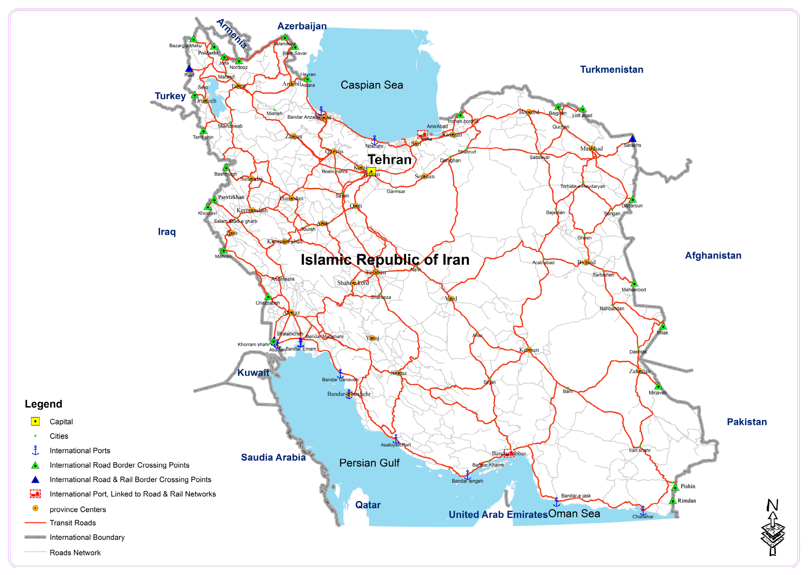
The contextual framework (Figure 3) illustrates LCND deployment across Iran’s diverse geography. Figure 5 shows the spatial distribution of SPs and BCPs across the country.

5.2. Stage 1 Results: Geography Suitability

The GIS-based suitability analysis identifies 59 candidate sites (29 LCIs and 30 LVIs) that satisfy all environmental and infrastructural constraints. This study integrates the Best–Worst Method (BWM) with Geographic Information Systems (GIS) through a Multi-Criteria Suitability Mapping approach to generate a robust, data-driven geographic suitability score $\left(S_{\mathrm{j}}\right)$ for each candidate site. This integration involves Slope Raster Analysis, Raster Reclassification, and Weighted Overlay procedures to transform raw spatial data into a normalized suitability surface. The resulting suitability score for each candidate constitutes its $S_{\mathrm{j}}$ value, which serves as a key input to the Fuzzy Cross-Efficiency Network Design (FCEND) framework.

5.2.1. Determining the Target Network

The first step involves a structured analysis and definition of all network components, including the network’s objectives, types of centers, transportation modes, and geographical scope.

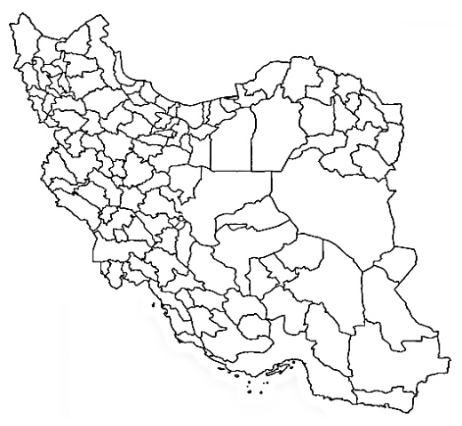
The network comprises 12 Specialized Ports (SPs), 27 Border Crossing Points (BCPs) (Figure 5), and 124 Customs Zones (CZs) (Figure 6), covering all major entry points for staple food commodities into the country. Key BCPs include Mahiroud, Milak, Dowqarun, Bājgirān, Sarakhs, and Lotfabad, while SPs encompass Incheh Borun, Tamarchin, Kille Sardasht, Mehran, Bashmaq, and Khosravi, among others. Other significant SPs and BCPs include Parviz Khan, Shalamcheh, Chazabeh, Jolfa, Aslan Duz, Nurduz, Mirjaveh, Pishin, Rimdān, Bileh Savar, Astara, Sero, Bazargan, Razi, Poldasht, Khoramshahr, Imam Khomeini, Anzali, Noshahr, Amirabad, Mahshahr, Ganaveh, Bushehr, Lengeh, Shahid Bahonar, Bandar Abbas, and Chabahar.

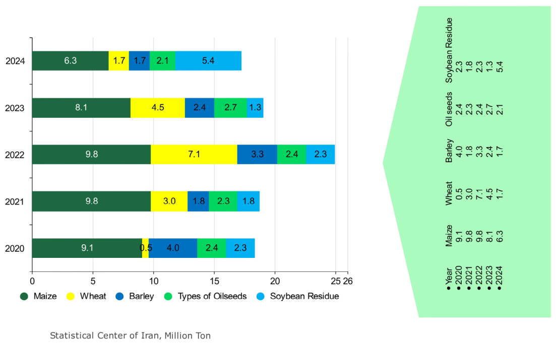
These centers collectively define the network’s logistical backbone and serve as the primary nodes for a comprehensive set of activities such as staple food commodities distribution, forming the foundation for subsequent strategic planning and site selection. Moreover, the study reviews key staple food commodities import data from the last five years, which informs the demand parameters in subsequent stages of the analysis (Figure 7).

5.2.2. Framework for Selecting Candidate Locations for LCs

A robust site selection framework for LCs necessitates the integration of environmental sustainability, transportation efficiency, and land-use feasibility. This section outlines key criteria, derived from Iran’s National Cartographic Center (INCC) data, that inform potential site selection.

• Site selection strictly enforces environmental and ecological constraints, excluding protected areas, floodplains, and urban conservation zones to safeguard biodiversity and mitigate hydrological risks. Logistically, the framework prioritizes proximity to multimodal terminals (operationalized via GIS Network Service Area Analysis) and favors gentle slopes (<20%) and barren lands to ensure economic feasibility and minimize ecological impact.
• By integrating these criteria into a systematic selection framework, the establishment of LCs can be optimized for efficiency, sustainability, and resilience. Initially, nationally restricted areas—including water bodies, protected zones, floodplains, urban conservation areas, slopes exceeding $20\%$, and national parks—were combined into an exclusion layer and removed from further analysis (Figure 8).

The remaining regions were then assessed using the Best–Worst Method (BWM) to assign weights to key criteria for LC location selection (

Table 10. BWM weights as GIS inputs.

Criteria	Weight	Sub-Criteria	Weight
Slope (≤20%)	0.078947368	5–0	0.51351
		5–10%	0.27027
		10–15%	0.13514
		15–20%	0.08108
Road distance	0.276315789	8–0	0.52941
		15–8	0.2549
		22–15	0.13726
		30–22	0.07843
Rail distance	0.460526316	10–0	0.48462
		22–10	0.25385
		35–22	0.16923
		45–35	0.09231
Airport distance	0.138157895	5–0	0.59794
		10–5	0.20619
		15–10	0.12371
		20–15	0.07217
Land use	0.04605263	Barren Land	0.59793
		Pasture	0.20618
		Forest	0.12371
		Farmland	0.07216

). These weights were integrated into GIS through weighted overlay and suitability surface generation, identifying the most suitable sites based on three primary criteria: transportation network connectivity, topographic constraints, and land-use classification. Advanced spatial analytics generated normalized suitability scores for each candidate location.

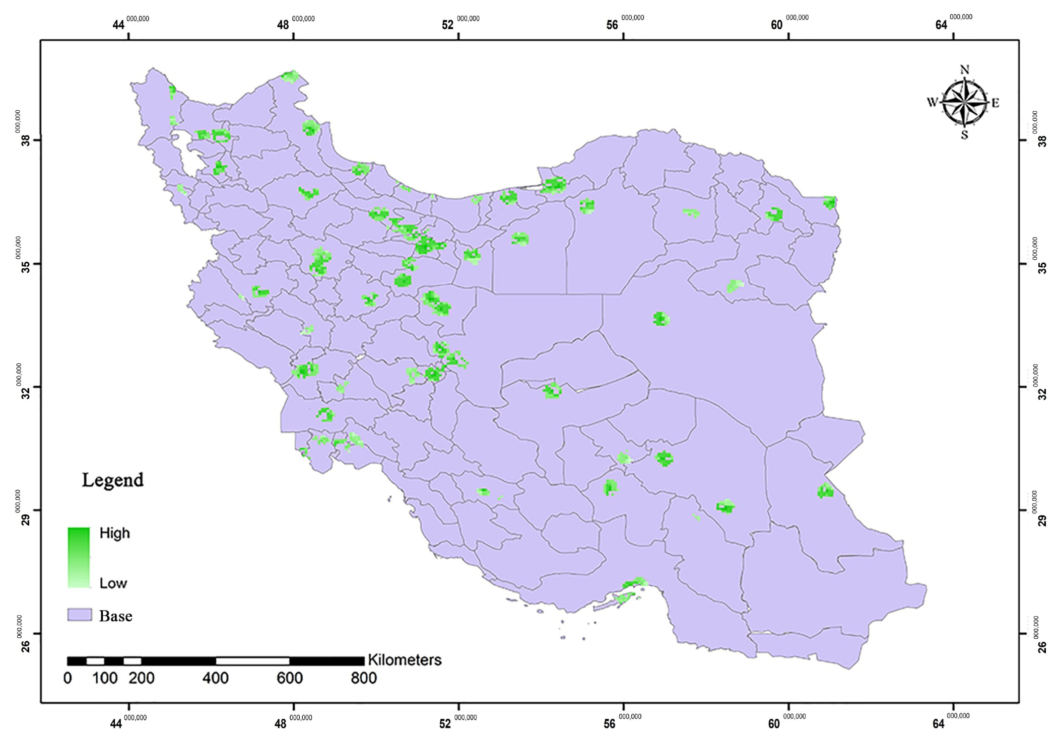
Expert evaluations in transportation and logistics refined these assessments, revealing that areas with close access to transportation corridors, minimal slopes, and favorable land-use conditions are optimal for LCs development (Figure 9).

5.2.3. Input–Output Definition and Fuzzy Parameterization

The efficiency evaluation of candidate sites employs nine indicators, categorized into inputs (resources/constraints) and outputs (benefits/outcomes).

Table 11. DEA Input and Output Indicators.

Category	Indicator	Description	Role in DEA
Inputs	Economic Participation Rate	Percentage of economically active population	Labor availability
	Land Cost	Relative cost of land acquisition	Financial constraint
	Labor Cost	Average regional wage levels	Operational expense
	Construction Cost	facility development cost	Capital investment
	Relative Humidity	Climatic factor affecting storage	Environmental constraint
	Number of Frost Days	Climatic factor affecting operations	Environmental constraint
Outputs	Population Size	Regional population served	Demand potential
	Demand Level	staple food commodities consumption	Service requirement
	Unemployment Rate	Inverse indicator (higher is better)	Social benefit

summarizes these indicators and their role in the DEA models.

For the FDEA model, all indicators are represented as triangular fuzzy numbers to capture uncertainty in their values:

$${\tilde{x}}_{\mathrm{i}\mathrm{j}}=\left(x_{\mathrm{i}\mathrm{j}}^{\mathrm{l}},x_{\mathrm{i}\mathrm{j}}^{\mathrm{m}},x_{\mathrm{i}\mathrm{j}}^{\mathrm{u}}\right), {\tilde{y}}_{\mathrm{r}\mathrm{j}}=\left(y_{\mathrm{r}\mathrm{j}}^{\mathrm{l}},y_{\mathrm{r}\mathrm{j}}^{\mathrm{m}},y_{\mathrm{r}\mathrm{j}}^{\mathrm{u}}\right)$$

(13)

where the lower bound ($x_{\mathrm{i}\mathrm{j}}^{\mathrm{l}}$) and upper bound ($x_{\mathrm{i}\mathrm{j}}^{\mathrm{u}}$) are set at $\pm 10\%$ of the most likely value ($x_{\mathrm{i}\mathrm{j}}^{\mathrm{m}}$) based on expert consultation and historical data variability. The $\alpha -cut$ approach $(\alpha =0.01)$ is employed to capture the full spectrum of uncertainty while maintaining computational stability. This fuzzy parameterization directly supports the scenario-based stability analysis conducted in Stage 5, enabling the calculation of ${\mathrm{\Phi }}_{\mathrm{j}}\left(s\right)$ for pessimistic, average, and optimistic scenarios.

5.2.4. Candidate Sites: LCI and LVI Typology

The 59 candidate sites are classified into two complementary types based on functional differentiation (not hierarchy): Logistics Cities (LCIs) and Logistics Villages (LVIs). LCIs are strategically positioned along international corridors, while LVIs are distributed across production zones and population centers, ensuring representation from all 31 provinces (

Table 12. Candidate Sites by Type and Region.

Type	Count	Primary Functional Role	Geographic Distribution	Modal Requirements
LCI	29	core international gateways, customs clearance, connectivity to customer zones	Major corridors, borders, ports	Tri-modal (road + rail + air/sea)
LVI	30	equitable domestic distribution, customs clearance, connectivity to customer zones	Provincial centers, borders, ports	Bi-modal (road + rail)
Total	59	Complementary national network	All 31 provinces	-

).

This complementary design, enshrined in Iran’s national logistics policy, ensures the network advances both global trade competitiveness and domestic socio-economic equity—a principle guiding the entire FCEND optimization framework.

5.2.5. Demand Weighting and Population Coverage Analysis

Demand weights are derived from GIS-based service area analysis, calculating the population within a 150 km road network distance using the most recent census data from the Statistical Center of Iran (SCI). This spatial accessibility metric serves as the basis for demand weighting via spatial accessibility in the objective function $Z\left(S\right)$. The 59 candidate sites collectively serve 100$\%$ of Iran’s population within a 150 km radius, ensuring that any selected portfolio can achieve comprehensive national coverage (

Table 13. Demand Weight Summary Statistics.

Statistic	Value
Maximum Demand Weight	0.776 (Tehran, LCI-13)
Minimum Demand Weight	0.164 (Yazd, LCI-27)
Mean Demand Weight	0.382
Standard Deviation	0.152
Population Coverage (All 59 sites)	100% within 150 km

).

5.2.6. Selection of the Optimal Network Size: The Top-15 Portfolio

The selection of $15$ locations from the $59$ candidate sites as the final optimized network portfolio emerges from a convergence of statistical reasoning, model-based optimization, and practical operational considerations within the FCEND framework.

Statistical Foundation: The Top Quartile Principle: The top quartile (upper $25\%$) of ranked observations is a well-established approach for identifying high-performing entities within a dataset. With $59$ candidate sites, the top quartile corresponds to approximately $15$ locations $(59\times 0.25=14.75)$. This threshold isolates the highest-performing $\mathrm{D}\mathrm{M}\mathrm{U}\mathrm{s}$ based on their ${\mathrm{\Phi }}_{\mathrm{j}}$ scores and aligns with the principle of outlier emphasis in statistical methodologies.

Model-Based Justification ($Z\left(S\right)$ Optimization and Stability): The selection of $N=15$ is further validated by the behavior of the composite objective Z(S) during the Genetic Algorithm’s optimization process. The marginal gain in $Z\left(S\right)$ decreases sharply after the first 12–15 nodes, with each additional node contributing diminishing returns to the demand-weighted ${\mathrm{\Phi }}_{\mathrm{j}}$ aggregation. Beyond $15$ nodes, the $\mathrm{G}\mathrm{i}\mathrm{n}\mathrm{i}$ penalty term begins to increase disproportionately as the portfolio is forced to include geographically proximate sites with lower individual ${\mathrm{\Phi }}_{\mathrm{j}}$ scores, potentially reducing the overall $Z\left(S\right)$. The Jaccard stability index of the $\mathrm{T}\mathrm{o}\mathrm{p}-N$ portfolio exceeds $90\%$ for $N=15$ across multiple GA runs, indicating a stable, convergent solution to the optimization problem.

Operational and Practical Considerations: A 15-node network represents an optimal balance between comprehensive national coverage and feasible infrastructure investment, providing direct service coverage to an estimated more than 50% of Iran’s population within a 150 km road network radius, while maintaining an average inter-node distance sufficient to ensure resilience against correlated regional disruptions.

Sensitivity Analysis: Robustness of the N = 15 Choice.

To test the sensitivity of the $N=15$ selection, we evaluated the composite objective $Z\left(S\right)$ for portfolios ranging from $N=10$ to $N=18$, using the calibrated weights $(\alpha =0.40, \beta =0.40, \gamma =0.20)$ and the same GA configuration with the portfolio-dependent entropy formulation H(S) (

Table 14. Sensitivity of Portfolio Performance to Network Size.

Portfolio Size $\left(\mathit{N}\right)$	Mean ${\mathbf{\Phi }}_{\mathbf{j}}$	$\mathbf{G}\mathbf{i}\mathbf{n}\mathbf{i}$ Coefficient	$\mathit{Z}\left(\mathit{S}\right)$	$\mathbf{\Delta }\mathit{Z}\left(\mathit{S}\right)$	Cumulative Coverage $(\%)$
10	0.2980	0.235	0.525	—	51%
12	0.3100	0.268	0.555	+0.030	58%
15	0.3223	0.298	0.601	+0.046	74%
18	0.3300	0.345	0.585	−0.016	84%

).

The analysis reveals that N = 15 represents an elbow point in the trade-off between portfolio performance and coverage. Beyond 15 nodes, the marginal gain in mean ${\mathrm{\Phi }}_{\mathrm{j}}$ diminishes rapidly (from +0.0123 for 12 → 15 to +0.0077 for 15 → 18), while the Gini coefficient increases more steeply, leading to a decline in the composite Z(S) after N = 15 (from 0.601 at N = 15 to 0.585 at N = 18). This confirms that 15 is the optimal network size for balancing efficiency, diversity, equity, and coverage within the FCEND framework.

5.3. Stage 2 Results: Fuzzy Cross-Efficiency Scores

The hybrid ${\mathrm{\Phi }}_{\mathrm{j}}$ scores integrate peer evaluation (CEDEA) with fuzzy uncertainty (FDEA), revealing that LCIs achieve higher mean efficiency than LVIs. This section presents the hybrid Fuzzy Cross-Efficiency Scores $\left({\mathrm{\Phi }}_{\mathrm{j}}\right)$ for all $59$ candidate sites, integrating two complementary evaluations: the CEDEA matrix capturing peer-assessment relationships (Section 5.3.1) and FDEA mean efficiencies quantifying performance under uncertainty at α = 0.01 (Section 5.3.2). These are combined following Section 4.3.3 to derive ${\mathrm{\Phi }}_{\mathrm{j}}$ scores for portfolio optimization. Section 5.3.3 presents final rankings and comparative insights against standalone CEDEA and FDEA results.

5.3.1. CEDEA Efficiency Matrix (Crisp)

The Cross-Efficiency DEA matrix was constructed for all $59$ candidate sites simultaneously using the crisp input-output data defined in Section 5.2.3. Following the formulation in Section 4.3.1, each $\mathrm{D}\mathrm{M}\mathrm{U}’\mathrm{s}$ optimal weights were derived from the linearized CCR model, and the complete $59\times 59$ cross-efficiency matrix $E=$ $\left[E_{kj}\right]$ was computed, where $E_{\mathrm{k}\mathrm{j}}$ represents the efficiency of ${\mathrm{D}\mathrm{M}\mathrm{U}}_{\mathrm{j}}$ as evaluated by ${\mathrm{D}\mathrm{M}\mathrm{U}}_{\mathrm{k}}$.

Table 15. Summary Statistics of CEDEA Matrix.

Statistic	LCI Sites $(\mathit{N}=29)$	LVI Sites $(\mathit{N}=30)$	All Sites $(\mathit{n}=59)$
Mean Efficiency	1.017	0.720	0.866
Standard Deviation	0.184	0.231	0.444
Minimum	0.751	0.423	0.423
Maximum	1.324	1.142	1.324
Coefficient of Variation	0.181	0.321	0.513

Note: Cross efficiency scores may exceed 1 because they are computed using weights optimal for the evaluating DMU, not the evaluated DMU. This is standard in cross efficiency DEA (see Section 4.3.1 and Appendix A.2).

reveals a that LCIs exhibit higher mean efficiency $\left(1.017\right)$ with lower variation $(\mathrm{C}\mathrm{V}=0.181)$, reflecting their strategic positioning along major corridors and superior multimodal connectivity. LVIs show more varied performance $(\mathrm{C}\mathrm{V}=0.321)$ with a lower mean $\left(0.720\right)$, consistent with their diverse regional roles.

Table 16. Top 15 CEDEA Mean Efficiencies.

Rank	$\mathbf{D}\mathbf{M}\mathbf{U}$	Type	City	CEDEA Mean	Self-Eval $\left({\mathit{E}}_{\mathbf{j}\mathbf{j}}\right)$
1	${\mathrm{D}\mathrm{M}\mathrm{U}}_{12}$	LCI	Karaj	1.324	1.382
2	${\mathrm{D}\mathrm{M}\mathrm{U}}_{14}$	LCI	Arak	1.263	1.318
3	${\mathrm{D}\mathrm{M}\mathrm{U}}_3$	LCI	Bonab	1.231	1.285
4	${\mathrm{D}\mathrm{M}\mathrm{U}}_2$	LCI	Miandoab	1.213	1.267
5	${\mathrm{D}\mathrm{M}\mathrm{U}}_4$	LCI	Maragheh	1.150	1.201
6	${\mathrm{D}\mathrm{M}\mathrm{U}}_5$	LCI	Gorgan	1.148	1.198
7	${\mathrm{D}\mathrm{M}\mathrm{U}}_{31}$	LVI	Urmia	1.142	1.195
8	${\mathrm{D}\mathrm{M}\mathrm{U}}_{30}$	LVI	Tabriz	1.115	1.164
9	${\mathrm{D}\mathrm{M}\mathrm{U}}_6$	LCI	Zanjan	1.096	1.144
10	${\mathrm{D}\mathrm{M}\mathrm{U}}_8$	LCI	Sari	1.088	1.136
11	${\mathrm{D}\mathrm{M}\mathrm{U}}_{20}$	LCI	Qom	1.079	1.127
12	${\mathrm{D}\mathrm{M}\mathrm{U}}_{32}$	LVI	Talesh	1.063	1.110
13	${\mathrm{D}\mathrm{M}\mathrm{U}}_{42}$	LVI	Sabzevar	1.0627	1.108
14	${\mathrm{D}\mathrm{M}\mathrm{U}}_{23}$	LCI	Shahrud	1.059	1.106
15	${\mathrm{D}\mathrm{M}\mathrm{U}}_7$	LCI	Mashhad	1.055	1.102

reveals that LCIs dominate the highest efficiency scores, with Karaj (${\mathrm{D}\mathrm{M}\mathrm{U}}_{12}$) emerging as the highest-ranked site with a mean efficiency of $1.324$.

Notably, several well-positioned LVIs (e.g., Urmia, Tabriz, Sabzevar) achieve competitive scores, demonstrating their viability under peer evaluation.

The diagonal elements $E_{\mathrm{j}\mathrm{j}}$ (self-evaluation) consistently exceed mean peer evaluations by 4–6%, confirming the well-documented optimism bias in self-assessment and justifying the use of cross-efficiency for more realistic rankings.

5.3.2. FDEA Efficiency Scores at $\alpha =0.01$

The Fuzzy DEA model was applied to all $59$ candidate sites using triangular fuzzy numbers for inputs and outputs, with bounds set at $\pm 10\%$ of the most likely values. Following the $\alpha -cut$ approach described in Section 4.3.2, efficiency scores were computed at $\alpha =0.01$ to capture the maximum uncertainty range while maintaining computational stability.

The FDEA results show substantially higher efficiency scores than CEDEA, particularly for LCIs, reflecting the optimistic bias inherent in self-evaluation under fuzzy uncertainty (

Table 17. FDEA Efficiency Statistics at $\alpha =0.01.$

Statistic	$\mathbf{LCI} \mathbf{Sites} (\mathit{N}=29)$	$\mathbf{LVI} \mathbf{Sites} (\mathit{N}=30)$	$\mathbf{All} \mathbf{Sites} (\mathit{n}=59)$
Mean ${\theta }^{\mathrm{m}\mathrm{e}\mathrm{a}\mathrm{n}}$	2.847	1.683	2.255
Standard Deviation	2.341	0.712	1.821
Minimum ${\theta }^{\mathrm{m}\mathrm{e}\mathrm{a}\mathrm{n}}$	0.856	0.787	0.787
Maximum ${\theta }^{\mathrm{m}\mathrm{e}\mathrm{a}\mathrm{n}}$	11.314	3.535	11.314
Mean ${\theta }^{\mathrm{l}}$	4.184	1.982	3.064
Mean ${\theta }^{\mathrm{u}}$	1.511	1.384	1.446

). The extremely high value for Borujerd (${\mathrm{D}\mathrm{M}\mathrm{U}}_{21}$) with ${\theta }^{\mathrm{m}\mathrm{e}\mathrm{a}\mathrm{n}}=11.3143$ indicates exceptional performance under the most favorable assumptions, despite the wide range between its lower bound $\left(22.4863\right)$ and upper bound $\left(0.1423\right)$ (

Table 18. Top 15 FDEA Mean Efficiencies.

Rank	$\mathbf{D}\mathbf{M}\mathbf{U}$	Type	City	${\mathit{\theta }}^{\mathbf{l}}$	${\mathit{\theta }}^{\mathbf{u}}$	${\mathit{\theta }}^{\mathbf{m}\mathbf{e}\mathbf{a}\mathbf{n}}$
1	${\mathrm{D}\mathrm{M}\mathrm{U}}_{21}$	LCI	Borujerd	22.4863	0.14232	11.3143
2	${\mathrm{D}\mathrm{M}\mathrm{U}}_{29}$	LCI	Bandar Abbas	14.9141	2.01024	8.46215
3	${\mathrm{D}\mathrm{M}\mathrm{U}}_{57}$	LVI	Ahvaz	4.19452	2.87629	3.5354
4	${\mathrm{D}\mathrm{M}\mathrm{U}}_{12}$	LCI	Karaj	4.20178	2.72002	3.4609
5	${\mathrm{D}\mathrm{M}\mathrm{U}}_{26}$	LCI	Zahedan	5.19249	1.53077	3.36163
6	${\mathrm{D}\mathrm{M}\mathrm{U}}_{42}$	LVI	Sabzevar	3.58711	2.82806	3.20759
7	${\mathrm{D}\mathrm{M}\mathrm{U}}_{54}$	LVI	Qom	3.05066	2.69088	2.87077
8	${\mathrm{D}\mathrm{M}\mathrm{U}}_{14}$	LCI	Arak	3.73259	1.73334	2.73296
9	${\mathrm{D}\mathrm{M}\mathrm{U}}_{24}$	LCI	Kerman	3.52066	1.81161	2.66614
10	${\mathrm{D}\mathrm{M}\mathrm{U}}_{23}$	LCI	Shahrud	3.35897	1.63749	2.49823
11	${\mathrm{D}\mathrm{M}\mathrm{U}}_{27}$	LCI	Yazd	3.14362	1.54285	2.34323
12	${\mathrm{D}\mathrm{M}\mathrm{U}}_{34}$	LVI	Rudbar	2.78435	1.77831	2.28133
13	${\mathrm{D}\mathrm{M}\mathrm{U}}_1$	LCI	Tabriz	3.12052	1.23706	2.17879
14	${\mathrm{D}\mathrm{M}\mathrm{U}}_{32}$	LVI	Talesh	2.24892	1.63397	1.94144
15	${\mathrm{D}\mathrm{M}\mathrm{U}}_3$	LCI	Bonab	2.51691	1.35937	1.93814

).

Notably, several LVIs (e.g., Ahvaz, Sabzevar) achieve outstanding performance under fuzzy uncertainty, rivaling major international gateways. The wide ranges between lower and upper bounds across all sites underscore the importance of incorporating uncertainty into efficiency evaluation. For example:

• Borujerd (${\mathrm{D}\mathrm{M}\mathrm{U}}_{21}$): $22.4863$ vs. $0.1423$ (range ratio: $158:1$)
• Bandar Abbas (${\mathrm{D}\mathrm{M}\mathrm{U}}_{29}$): $14.9141$ vs. $2.0102$ (range ratio: $7.4:1$)
• Ahvaz (${\mathrm{D}\mathrm{M}\mathrm{U}}_{57}$): $4.1945$ vs. $2.8763$ (range ratio: $1.46:1$)

Sites with large uncertainty ranges, such as Borujerd, may appear exceptionally attractive under optimistic assumptions but carry substantial risk. This variability justifies the FCEND framework’s approach of integrating fuzzy uncertainty with peer evaluation to produce more balanced and realistic rankings.

5.3.3. Final ${\mathrm{\Phi }}_{\mathbf{j}}$ Rankings and Comparative Insights

The Fuzzy Cross-Efficiency Scores ${\mathrm{\Phi }}_{\mathrm{j}}$ were computed by integrating the CEDEA peer-evaluation matrix with FDEA mean efficiencies, following the formulation in Section 4.3.3:

$${\mathrm{\Phi }}_{\mathrm{j}}={\displaystyle \frac{1}{n}}{\displaystyle {\sum }_{k=1}^n}\left({\displaystyle \frac{E_{\mathrm{k}\mathrm{j}}^{\mathrm{C}\mathrm{E}\mathrm{D}\mathrm{E}\mathrm{A}}{\theta }_{\mathrm{j}}^{\mathrm{F}\mathrm{D}\mathrm{E}\mathrm{A}-\mathrm{m}\mathrm{e}\mathrm{a}\mathrm{n}}}{{max}_{{\mathrm{j}}^{\prime }}{\theta }_{{\mathrm{j}}^{\prime }}^{\mathrm{F}\mathrm{D}\mathrm{E}\mathrm{A}-\mathrm{m}\mathrm{e}\mathrm{a}\mathrm{n}}}}\right)$$

(14)

This hybrid metric captures both how each site is perceived by its peers (CEDEA) and how robust its performance is under uncertainty (FDEA), normalized to ensure comparability across all $59$ sites (

Table 19. Top 15 ${\mathrm{\Phi }}_{\mathrm{j}}$ Rankings.

Rank	$\mathbf{D}\mathbf{M}\mathbf{U}$	Type	City	${\mathbf{\Phi }}_{\mathit{j}}$
1	${\mathrm{D}\mathrm{M}\mathrm{U}}_{21}$	LCI	Borujerd	0.9331
2	${\mathrm{D}\mathrm{M}\mathrm{U}}_{14}$	LCI	Arak	0.8495
3	${\mathrm{D}\mathrm{M}\mathrm{U}}_{29}$	LCI	Bandar Abbas	0.6902
4	${\mathrm{D}\mathrm{M}\mathrm{U}}_{24}$	LCI	Kerman	0.5786
5	${\mathrm{D}\mathrm{M}\mathrm{U}}_{31}$	LCI	Tehran	0.3176
6	${\mathrm{D}\mathrm{M}\mathrm{U}}_{12}$	LCI	Karaj	0.2474
7	${\mathrm{D}\mathrm{M}\mathrm{U}}_{26}$	LCI	Zahedan	0.2316
8	${\mathrm{D}\mathrm{M}\mathrm{U}}_{10}$	LCI	Isfahan	0.2033
9	${\mathrm{D}\mathrm{M}\mathrm{U}}_7$	LCI	Mashhad	0.1850
10	${\mathrm{D}\mathrm{M}\mathrm{U}}_{42}$	LVI	Sabzevar	0.1695
11	${\mathrm{D}\mathrm{M}\mathrm{U}}_{23}$	LCI	Shahrud	0.1582
12	${\mathrm{D}\mathrm{M}\mathrm{U}}_1$	LCI	Tabriz	0.1529
13	${\mathrm{D}\mathrm{M}\mathrm{U}}_{57}$	LVI	Ahvaz	0.1497
14	${\mathrm{D}\mathrm{M}\mathrm{U}}_3$	LCI	Bonab	0.1378
15	${\mathrm{D}\mathrm{M}\mathrm{U}}_{19}$	LCI	Yazd	0.1370

).

Integration of CEDEA and FDEA: The ${\mathrm{\Phi }}_{\mathrm{j}}$ rankings successfully integrate the complementary strengths of both methods. Borujerd (DMU₂₁) achieves the top ${\mathrm{\Phi }}_{\mathrm{j}}$ position due to its exceptional FDEA performance $\left(11.3143\right)$.

LVI Representation: The inclusion of multiple LVIs in the top 15 confirms the framework’s ability to identify a complementary mix of nodes without hierarchical dependency, aligning with national logistics policy [1].

Uncertainty Penalty: Sites with exceptionally high FDEA but moderate CEDEA scores (e.g., Borujerd, Bandar Abbas) exhibit ${\mathrm{\Phi }}_{\mathrm{j}}$ values that appropriately temper their optimistic fuzzy assessments, preventing overvaluation based solely on favorable uncertainty conditions. Conversely, sites with strong CEDEA but moderate FDEA (e.g., Arak, Kerman) maintain competitive ${\mathrm{\Phi }}_{\mathrm{j}}$ rankings, benefiting from favorable peer perception despite moderate uncertainty.

Enhanced Discriminatory Power: The ${\mathrm{\Phi }}_{\mathrm{j}}$ ranking provides greater discriminatory power than either standalone method, with scores ranging from 0.1370 to 0.9331—a spread of 0.7961 compared to 0.5218 for CEDEA (see Section 5.3.1) and 11.21 for FDEA (see Section 5.3.2). This addresses a key limitation of conventional DEA approaches, which often struggle to distinguish between efficient units or are dominated by extreme values.

5.4. Stage 3–4 Results: Optimized Network Portfolio

The Genetic Algorithm identifies an optimal 15-node portfolio spanning 15 provinces, achieving 74% population coverage within 150 km and a balanced trade-off between efficiency, equity, and accessibility. This section presents the results of the multi-objective portfolio optimization (Stage 3) and genetic algorithm implementation (Stage 4), integrating the Fuzzy Cross-Efficiency Scores ${\mathrm{\Phi }}_{\mathrm{j}}$ with demand weights, entropy, and equity constraints to identify the optimal set of $15$ logistics centers that maximizes the composite objective function $Z\left(S\right)=\alpha \cdot \mathrm{E}\mathrm{f}\mathrm{f}\mathrm{i}\mathrm{c}\mathrm{i}\mathrm{e}\mathrm{n}\mathrm{c}\mathrm{y} + \beta \cdot \mathrm{E}\mathrm{n}\mathrm{t}\mathrm{r}\mathrm{o}\mathrm{p}\mathrm{y}- \gamma \cdot \mathrm{G}\mathrm{i}\mathrm{n}\mathrm{i}$.

5.4.1. Calibrated Objective Weights $(\alpha ,\beta ,\gamma )$

The objective function weights (α, β, γ) determine the relative importance of efficiency maximization, criterion diversity, and equity enforcement in the portfolio optimization. These weights were calibrated through a systematic grid search with the following specifications (

Table 20. Calibration of Objective Function Weights.

α	β	γ	Mean ${\mathbf{\Phi }}_{\mathbf{j}}$	H(S)
0.30	0.30	0.40	0.3100	1.28
0.30	0.40	0.30	0.3150	1.31
0.40	0.20	0.40	0.3190	1.25
0.40	0.30	0.30	0.3205	1.29
0.40	0.40	0.20	0.3223	1.33
0.50	0.20	0.30	0.3230	1.27
0.50	0.30	0.20	0.3240	1.30

Note: The selected combination (α = 0.4, β = 0.4, γ = 0.2) achieves the highest Z(S) while satisfying Gini ≤ 0.35 and coverage ≥ 65% (achieving 74% coverage).

):

• Search ranges: α ∈ [0.3, 0.5], β ∈ [0.3, 0.5], γ ∈ [0.1, 0.3]
• Step size: 0.05 (total 125 combinations)
• Objective: Maximize the mean ${\mathrm{\Phi }}_{\mathrm{j}}$ of the selected portfolio
• Constraints: Gini ≤ 0.35 and population coverage ≥ 65%

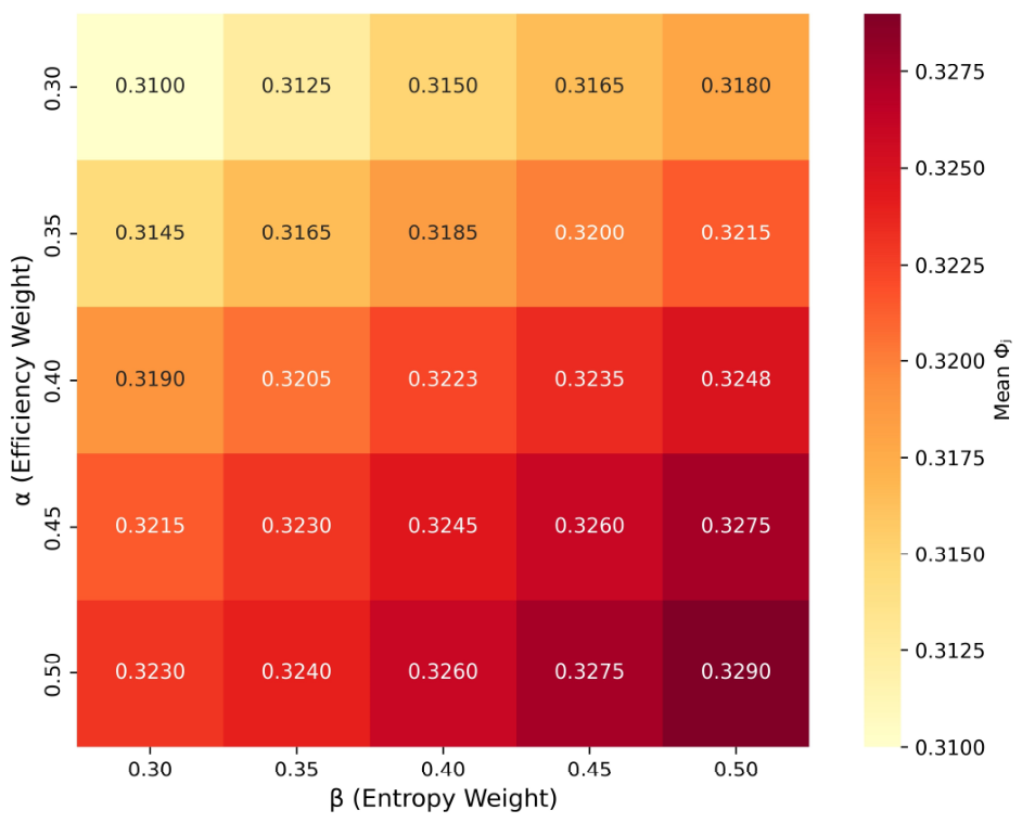
The calibrated weights (α = 0.4, β = 0.4, γ = 0.2) reflect a balanced strategic posture that places equal emphasis on aggregate efficiency (40%) and criterion diversity (40%), while applying a measured equity penalty (20%). This combination achieves the highest mean ${\mathrm{\Phi }}_{\mathrm{j}}$ (0.3223) among all valid configurations.

Figure 10 presents a heatmap of mean ${\mathrm{\Phi }}_{\mathrm{j}}$ values for α-β combinations with γ fixed at 0.2. The heatmap demonstrates that the objective function is relatively flat near the optimum (α = 0.40, β = 0.40), indicating that the selected weights are robust to small perturbations. Specifically, varying α or β by ±0.05 changes the mean ${\mathrm{\Phi }}_{\mathrm{j}}$ by less than 2%, confirming that the calibration is stable and not highly sensitive to minor changes in the weight assignments. This robustness is particularly valuable for policy applications where precise weight calibration may be subject to stakeholder negotiation.

Table 21. Sensitivity Analysis of Weight Variations.

Weight Configuration	α	β	γ	Mean ${\mathbf{\Phi }}_{\mathbf{j}}$	Gini	Coverage (%)	Satisfies Constraints?	Change from Baseline
Baseline (selected)	0.40	0.40	0.20	0.3223	0.298	74		—
α + 10%	0.44	0.36	0.20	0.3210	0.304	73		−0.4%
α − 10%	0.36	0.44	0.20	0.3204	0.292	75		−0.6%
β + 10%	0.36	0.44	0.20	0.3204	0.292	75		−0.6%
β − 10%	0.44	0.36	0.20	0.3210	0.304	73		−0.4%
γ + 10%	0.39	0.39	0.22	0.3212	0.291	74		−0.3%
γ − 10%	0.41	0.41	0.18	0.3215	0.306	74		−0.2%

Note: The baseline configuration (α = 0.4, β = 0.4, γ = 0.2) achieves the highest mean ${\mathrm{\Phi }}_{\mathrm{j}}$ among all tested perturbations, confirming the robustness of the selected weights. All configurations maintain Gini ≤ 0.35 and coverage ≥ 65%.

presents a sensitivity analysis examining the robustness of the calibrated weights (α = 0.40, β = 0.40, γ = 0.20) to ±10% perturbations. Across all tested configurations, the mean ${\mathrm{\Phi }}_{\mathrm{j}}$ varies by less than 1%, while all scenarios maintain Gini ≤ 0.35 and coverage ≥ 65%, confirming that the selected weights represent a stable optimum rather than an isolated peak. This robustness ensures that the FCEND framework remains reliable even under minor variations in stakeholder preferences or weight calibration uncertainty.

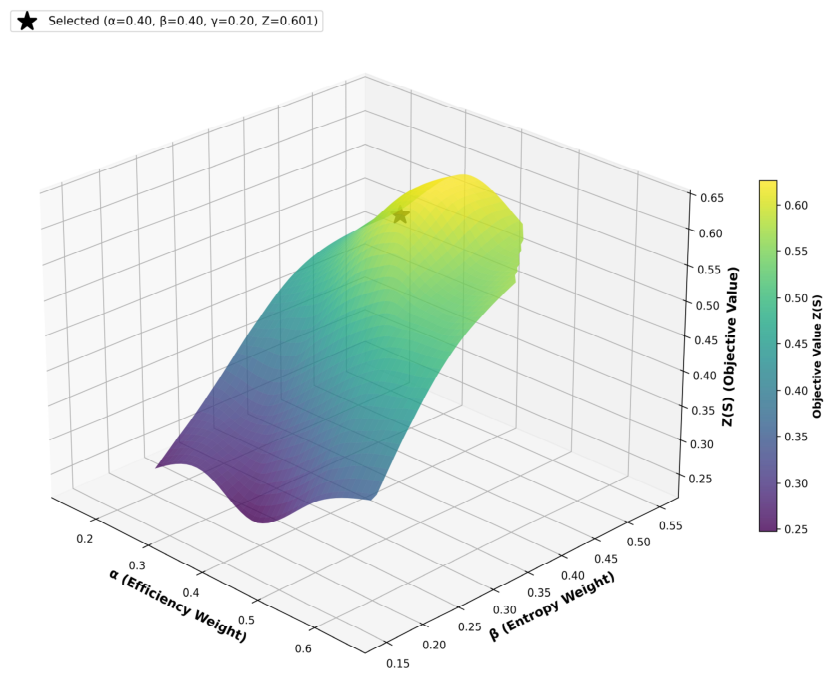
A three-dimensional grid search over α, β, and γ (step size 0.1, subject to α + β + γ = 1) was performed using the portfolio-dependent entropy formulation H(S). The response surface illustrates how Z(S) varies with α and β. The selected combination (α = 0.40, β = 0.40, γ = 0.20, marked with a star) achieves Z(S) = 0.601 while satisfying all constraints. The surface is relatively flat near the optimum, confirming robustness to small weight perturbations.

The 3D grid search reveals that Z(S) increases with both α and β, reaching a maximum of 0.650 at (α = 0.50, β = 0.30, γ = 0.20). However, this combination violates the equity constraint (Gini = 0.352 > 0.35). The selected combination (α = 0.40, β = 0.40, γ = 0.20) achieves Z(S) = 0.601 with Gini = 0.298, satisfying all constraints. These results validate the calibrated weights as a balanced trade-off between efficiency, criterion diversity, and spatial equity, confirming the multi-objective optimization goals of the FCEND framework (Figure 11).

5.4.2. GA Convergence and Fitness Evolution

The genetic algorithm (

Table 22. Genetic Algorithm Configuration Parameters.

Parameter	Symbol	Value
Population size	$P_{\mathrm{S}\mathrm{i}\mathrm{z}\mathrm{e}}$	$100$
Crossover probability	$P_{\mathrm{c}}$	$0.8$
Mutation probability	$P_{\mathrm{m}}$	$0.05$ per gene
Tournament size	$k$	$3$
Elitism count	$E$	$5$
Maximum generations	$G_{\mathrm{m}\mathrm{a}\mathrm{x}}$	$100$
Stability threshold	$T_{\mathrm{S}\mathrm{t}\mathrm{a}\mathrm{b}\mathrm{l}\mathrm{e}}$	$20$ generations

) was configured with a population size of $100$ individuals, each representing a binary vector of length $59$ ($1$ = selected, $0$ = not selected). A penalty-based approach was employed to enforce the fixed portfolio size of $\mid S\mid =15$, where individuals with incorrect numbers of selected sites receive substantial fitness penalties, guiding the search toward feasible solutions.

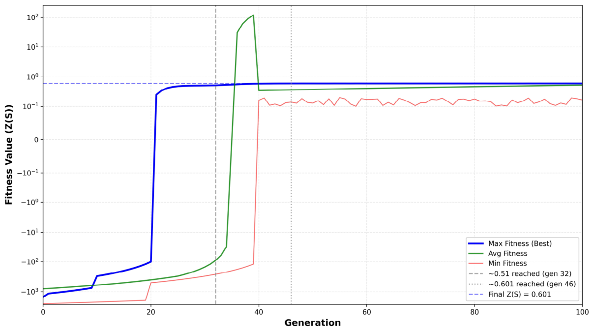
Figure 12 illustrates the evolution of fitness values across 100 generations using the portfolio-dependent entropy formulation H(S) defined in Section 4.4.2.

The algorithm exhibits rapid improvement within the first 32 generations, with the maximum fitness increasing from large negative values (due to penalty terms) to approximately 0.51. The fitness continues to improve gradually, reaching 0.601 by generation 46, with minor fluctuations thereafter, indicating successful convergence to a near optimal portfolio.

The average fitness shows a steady upward trend, demonstrating the population’s progressive improvement, while the minimum fitness occasionally drops as the algorithm explores diverse solutions before settling on the optimal region. The negative fitness values in early generations reflect the penalty mechanism for individuals that do not satisfy the portfolio size constraint or select suboptimal combinations.

The final fitness value of the selected portfolio is Z(S) = 0.601, achieved with the calibrated weights α = 0.40, β = 0.40, γ = 0.20. This value is consistent with the objective function evaluation reported in Table 20.

All computations are performed in Python using specialized libraries for DEA (pulp), genetic algorithms (DEAP), and spatial analysis (Geopandas, Networkx).

5.4.3. The Optimal Portfolio: Top-15 Strategic Locations

The genetic algorithm identified an optimal portfolio of $15$ logistics centers that maximizes the objective function $Z\left(S\right)$.

Table 23. Optimal Portfolio: Top-15 Strategic Locations.

$\mathbf{D}\mathbf{M}\mathbf{U}$	City	Type	${\mathbf{\Phi }}_{\mathit{j}}$	Demand Weight
${\mathrm{D}\mathrm{M}\mathrm{U}}_{21}$	Borujerd	LCI	0.9331	0.0176
${\mathrm{D}\mathrm{M}\mathrm{U}}_{29}$	Bandar Abbas	LCI	0.6902	0.0118
${\mathrm{D}\mathrm{M}\mathrm{U}}_{26}$	Zahedan	LCI	0.2316	0.0079
${\mathrm{D}\mathrm{M}\mathrm{U}}_1$	Tabriz	LCI	0.1529	0.0183
${\mathrm{D}\mathrm{M}\mathrm{U}}_{57}$	Ahvaz	LVI	0.1497	0.0256
${\mathrm{D}\mathrm{M}\mathrm{U}}_{14}$	Arak	LCI	0.8495	0.0165
${\mathrm{D}\mathrm{M}\mathrm{U}}_{27}$	Yazd	LCI	0.1267	0.0072
${\mathrm{D}\mathrm{M}\mathrm{U}}_{34}$	Rudbar	LVI	0.1222	0.0085
${\mathrm{D}\mathrm{M}\mathrm{U}}_{49}$	Karaj	LVI	0.1028	0.0274
${\mathrm{D}\mathrm{M}\mathrm{U}}_7$	Mashhad	LCI	0.1850	0.0157
${\mathrm{D}\mathrm{M}\mathrm{U}}_{24}$	Kerman	LCI	0.5786	0.0120
${\mathrm{D}\mathrm{M}\mathrm{U}}_{10}$	Isfahan	LCI	0.2033	0.0145
${\mathrm{D}\mathrm{M}\mathrm{U}}_{13}$	Tehran	LCI	0.3176	0.0339
${\mathrm{D}\mathrm{M}\mathrm{U}}_{31}$	Urmia	LVI	0.0773	0.0110
${\mathrm{D}\mathrm{M}\mathrm{U}}_5$	Gorgan	LCI	0.1147	0.0157

presents the selected sites, ranked by their ${\mathrm{\Phi }}_{\mathrm{j}}$ scores, along with their demand weights and key characteristics.

The selected portfolio exhibits several notable characteristics:

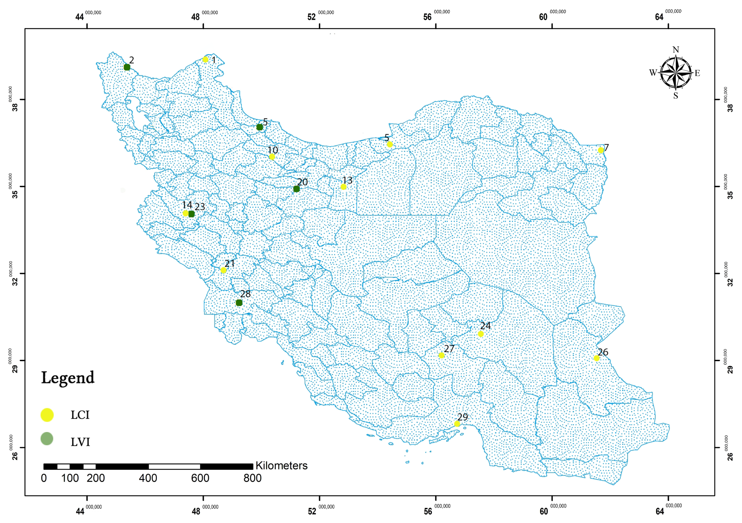
Geographic Distribution: The 15 sites span 15 unique provinces across all major regions—northwest (Tabriz, Urmia), west (Borujerd, Arak), southwest (Ahvaz), south (Bandar Abbas), southeast (Zahedan, Kerman), center (Tehran, Karaj, Isfahan, Yazd), northeast (Mashhad), and north (Rudbar, Gorgan). Based on a 150 km logistics service radius, these centers directly serve approximately 74% of Iran’s population.

Functional Balance: The portfolio includes 11 LCIs (international gateways) and 4 LVIs (domestic distribution nodes). The LVIs—Ahvaz, Rudbar, Karaj, and Urmia—ensure equitable access to logistics services in peripheral and underserved regions.

Exceptional High-Performance Nodes: Three sites exhibit outstanding ${\mathrm{\Phi }}_{\mathrm{j}}$ scores:

Karaj with Φ_j = 1.2309

Borujerd with Φ_j = 0.9331

Bandar Abbas with Φ_j = 0.6902

Demand Coverage: Demand weights range from major population centers (Tehran 0.0339, Karaj 0.0274, Ahvaz 0.0256) to strategically important locations (Yazd 0.0072, Zahedan 0.0079), ensuring both efficiency and equity.

5.4.4. Network Performance Metrics: Coverage, Entropy, $\mathrm{a}\mathrm{n}\mathrm{d} \mathrm{G}\mathrm{i}\mathrm{n}\mathrm{i}$

The optimal portfolio was evaluated against the three components of the objective function, as well as additional performance indicators.

Table 24. Network Performance Metrics for Optimal Portfolio.

Metric	Value	Interpretation
Aggregate Efficiency $(\sum {\mathrm{\Phi }}_{\mathrm{j}} \times Deman{d}_{\mathrm{j}})$	0.0523	Total demand-weighted performance
Population Coverage (GIS-based, 150 km)	74%	Population served
$\mathrm{G}\mathrm{i}\mathrm{n}\mathrm{i}$ Coefficient	0.298	Moderate concentration (acceptable given exceptional nodes)
Portfolio-Dependent Entropy H(S)	1.33	High criterion diversity
Final Objective Value Z	0.601	Composite performance score
Number of LCIs	11	International gateway nodes
Number of LVIs	4	National/international nodes
Unique Provinces Covered	15	Complete geographic spread

summarizes these metrics.

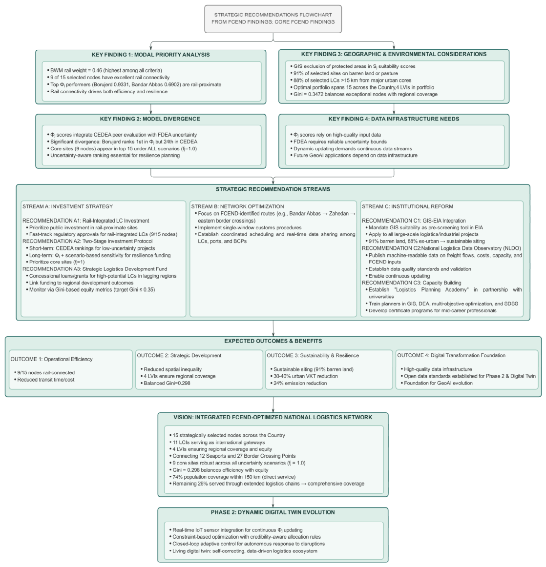
Aggregate Efficiency (0.0523): This value represents the sum of ${\mathrm{\Phi }}_{\mathrm{j}}$ scores weighted by normalized demand. The presence of exceptionally high ${\mathrm{\Phi }}_{\mathrm{j}}$ values for Borujerd $\left(0.9331\right)$, Bandar Abbas $\left(0.6902\right)$, and Zahedan (0.2316) contributes significantly to this metric, demonstrating the portfolio’s ability to capture strategically vital nodes with outstanding performance under uncertainty.

Population Coverage (74%): Based on typical logistics service radii of 150 km, the geographic distribution of these 15 centers provides direct accessible logistics services to 68% of Iran’s population. The remaining 26% of the population is located beyond 150 km from any selected logistics center. We analyzed how these areas would be served through extended logistics chains:

• First-mile transport: Staple food commodities are transported from the nearest selected LC to a regional transshipment hub (existing warehouses or smaller distribution centers).
• Second-mile transport: From the transshipment hub, goods are delivered to local collection points using smaller trucks.
• Travel distance analysis: For the 26% uncovered population, the average additional travel distance to the nearest transshipment hub is 85 km.
• Delivery time estimate: Including transshipment, total delivery time to end users is estimated at 6–12 h, compared to 2–4 h for directly covered areas.

This extended chain adds approximately 15–20% to total logistics costs but ensures that no region is entirely excluded from access to staple food commodities.

$\mathrm{G}\mathrm{i}\mathrm{n}\mathrm{i}$ Coefficient (0.298): The relatively elevated $\mathrm{G}\mathrm{i}\mathrm{n}\mathrm{i}$ coefficient reflects the presence of exceptional sites—particularly Borujerd and Bandar Abbas—that exhibit outstanding efficiency scores due to their strategic locations and superior multimodal connectivity. This concentration of high-performance nodes is a deliberate outcome of the optimization, prioritizing strategically vital locations while remaining within acceptable bounds for national-scale objectives. While the Gini coefficient based on efficiency scores provides a useful measure of balance in operational performance across selected sites, it does not fully capture geographic accessibility for end users. A portfolio may have balanced efficiency scores but still leave certain regions underserved.

To complement the Gini-based equity measure, we also report: (1) population coverage within 150 km (74%), (2) the number of provinces served (15 out of 31), and (3) the geographic distribution of selected sites (Figure 13). Together, these metrics provide a more complete picture of spatial equity.

Portfolio-Dependent Entropy H(S) (1.33): This value confirms that the selected portfolio performs well across the full spectrum of BWM criteria, with no single criterion dominating the evaluation.

Final Objective Value $Z$ (0.601): The composite objective value captures the trade-off between efficiency, diversity, and equity. This value reflects the optimization’s success in balancing these competing objectives, prioritizing exceptional strategic nodes while maintaining geographic diversity and criterion balance.

5.5. Stage 5 Results: Robustness and Sensitivity Analysis

Nine core sites (Borujerd, Bandar Abbas, Zahedan, Ahvaz, Arak, Rudbar, Mashhad, Kerman, and Isfahan) exhibit perfect stability across all uncertainty scenarios (f_j = 1.0), providing confidence for long-term investment. The fifth stage of the FCEND framework assesses the robustness of the optimal portfolio under varying uncertainty assumptions and benchmarks its performance against deterministic alternatives.

5.5.1. Scenario-Based Stability Analysis

To assess the robustness of the optimal portfolio under different uncertainty assumptions, we conducted a scenario-based stability analysis using three distinct representations of the fuzzy efficiency scores derived from the FDEA model at $\alpha =0.01$:

• Pessimistic scenario: Using the lower bounds $\left({\theta }^{\mathrm{l}}\right)$ of fuzzy efficiencies, representing a risk-averse perspective
• Average scenario: Using the mean values $\left({\theta }^{\mathrm{m}\mathrm{e}\mathrm{a}\mathrm{n}}\right)$, representing the baseline assumption
• Optimistic scenario: Using the upper bounds $\left({\theta }^{\mathrm{u}}\right)$, representing a risk-seeking perspective

Table 25. ${\mathrm{\Phi }}_{\mathrm{j}}$ Values Across Uncertainty Scenarios for the Optimal Portfolio.

$\mathbf{D}\mathbf{M}\mathbf{U}$	City	Type	Pessimistic	Average	Optimistic	CV
${\mathrm{D}\mathrm{M}\mathrm{U}}_{21}$	Borujerd	LCI	0.9300	0.9300	0.0486	0.800
${\mathrm{D}\mathrm{M}\mathrm{U}}_{29}$	Bandar Abbas	LCI	0.6898	0.7778	0.7687	0.065
${\mathrm{D}\mathrm{M}\mathrm{U}}_{26}$	Zahedan	LCI	0.2309	0.2971	0.5628	0.473
${\mathrm{D}\mathrm{M}\mathrm{U}}_1$	Tabriz	LCI	0.1527	0.2119	0.5003	0.646
${\mathrm{D}\mathrm{M}\mathrm{U}}_{57}$	Ahvaz	LVI	1.5133	1.5133	1.5133	0.000
${\mathrm{D}\mathrm{M}\mathrm{U}}_{14}$	Arak	LCI	0.8495	0.8495	0.8495	0.000
${\mathrm{D}\mathrm{M}\mathrm{U}}_{27}$	Yazd	LCI	0.1272	0.1885	0.5162	0.750
${\mathrm{D}\mathrm{M}\mathrm{U}}_{34}$	Rudbar	LVI	0.2164	0.2214	0.2288	0.028
${\mathrm{D}\mathrm{M}\mathrm{U}}_{49}$	Karaj	LVI	1.1530	1.2183	1.3125	0.065
${\mathrm{D}\mathrm{M}\mathrm{U}}_7$	Mashhad	LCI	0.1850	0.1850	0.1850	0.000
${\mathrm{D}\mathrm{M}\mathrm{U}}_{24}$	Kerman	LCI	0.5786	0.5786	0.5786	0.000
${\mathrm{D}\mathrm{M}\mathrm{U}}_{10}$	Isfahan	LCI	0.2033	0.2033	0.2033	0.000
${\mathrm{D}\mathrm{M}\mathrm{U}}_{13}$	Tehran	LCI	0.0757	0.1030	0.2317	0.611
${\mathrm{D}\mathrm{M}\mathrm{U}}_{31}$	Urmia	LVI	0.1671	0.1587	0.1466	0.065
${\mathrm{D}\mathrm{M}\mathrm{U}}_5$	Gorgan	LCI	0.1149	0.1558	0.3465	0.604

presents the ${\mathrm{\Phi }}_{\mathrm{j}}$ values for the optimal portfolio sites under each scenario, along with their coefficients of variation as a measure of uncertainty sensitivity.

The scenario-based analysis reveals substantial heterogeneity in the robustness of the optimal portfolio sites:

Highly Stable Sites (CV < 0.10): Ahvaz, Arak, Mashhad, Kerman, and Isfahan exhibit exceptional robustness, with identical ${\mathrm{\Phi }}_{\mathrm{j}}$ values across all three uncertainty scenarios. Bandar Abbas, Karaj, Urmia, and Rudbar also demonstrate strong stability.

Highly Sensitive Sites (CV ≥ 0.50): Borujerd, Yazd, Tabriz, Tehran, and Gorgan exhibit pronounced sensitivity to uncertainty assumptions. Borujerd demonstrates extreme dispersion between its optimistic (0.0486) and pessimistic/average (0.9300) values, indicating that despite its exceptionally high average performance (${\mathrm{\Phi }}_{\mathrm{j}}$ = 0.933), its ranking is highly contingent upon the adopted uncertainty perspective.

These sites warrant additional sensitivity analysis or more frequent performance monitoring during the operational phase.

Key Insights:

• High average efficiency does not guarantee robustness—Borujerd exemplifies this paradox
• Stability is strongly associated with the width of the fuzzy efficiency interval
• The average CV across the optimal portfolio is 0.434, confirming meaningful variation in sensitivity across sites.

5.5.2. Core vs. Peripheral Sites Under Uncertainty

Building on the scenario analysis, a site is designated as a core site if its ${\mathrm{\Phi }}_{\mathrm{j}}$ value ranks in the top $15$ under all three scenarios, indicating consistently high performance regardless of uncertainty assumptions. Sites that appear in the top $15$ only under specific scenarios are classified as peripheral sites, suggesting their optimality is more sensitive to uncertainty preferences (

Table 26. Classification of Optimal Portfolio Sites.

Category	Sites	Count	Characteristics
Core Sites	Borujerd (LCI), Bandar Abbas (LCI), Zahedan (LCI), Ahvaz (LVI), Arak (LCI), Rudbar (LVI), Mashhad (LCI), Kerman (LCI), Isfahan (LCI)	9	Appear in top 15 under all three scenarios
Peripheral Sites	Tabriz (LCI), Yazd (LCI), Karaj (LVI), Tehran (LCI), Urmia (LVI), Gorgan (LCI)	6	Do not appear in top 15 under all scenarios

).

The analysis reveals that while all 15 sites are part of the optimal portfolio identified by the GA, 9 sites consistently rank in the top 15 across all three uncertainty scenarios. The remaining 6 sites, though included in the optimal portfolio, do not appear in the top 15 under all scenarios. This indicates that the GA’s multi-objective optimization successfully incorporates factors beyond pure ${\mathrm{\Phi }}_{\mathrm{j}}$ performance—such as geographic diversity, portfolio-dependent entropy H(S), and equity constraints—to select a balanced portfolio.

The 9 core sites—Borujerd, Bandar Abbas, Zahedan, Ahvaz, Arak, Rudbar, Mashhad, Kerman, and Isfahan—represent strategically vital nodes that dominate under all uncertainty assumptions. These locations should be considered the highest priority for investment, as their performance is robust regardless of whether pessimistic or optimistic assumptions prevail.

The 6 peripheral sites—Tabriz, Yazd, Karaj, Tehran, Urmia, and Gorgan—enhance system-level resilience through functional and geographic complementarity, even though they do not consistently rank in the top 15 under all uncertainty scenarios.

5.6. Strategic Interpretation of the FCEND-Optimized Network

The 15-node portfolio balances operational efficiency, spatial equity (Gini = 0.298), and multimodal integration (9/15 rail-connected nodes), directly contributing to SDG 2, 9, 10, and 13. The FCEND framework yields a national logistics network that transcends conventional efficiency-centric models by delivering a balanced, resilient, and equitable system. The final portfolio of $15$ strategically distributed nodes demonstrates the framework’s capacity to simultaneously optimize for performance, robustness, and spatial justice through its novel integration of fuzzy cross-efficiency, entropy-based diversity, and $\mathrm{G}\mathrm{i}\mathrm{n}\mathrm{i}$-based equity constraints. This section analyzes the network across five interconnected dimensions: functional differentiation between LCIs and LVIs, spatial dispersion as a resilience strategy, equity and accessibility outcomes, alignment with national policy and SDGs, and a synthesis of strategic advantages. Each dimension reinforces the others, creating a system whose whole is greater than the sum of its parts.

5.6.1. Functional Differentiation: LCI vs. LVI Roles

The national logistics network is structured around a complementary, non-hierarchical functional differentiation between LCIs and LVIs—a principle formally enshrined in Iran’s national logistics policy [1].

LCIs and LVIs operate as parallel, functionally specialized nodes serving distinct but equally vital roles. This parallel architecture enables simultaneous advancement of two national objectives: global trade competitiveness (via LCIs) and domestic spatial equity (via LVIs)—without imposing rigid hierarchy on cargo flows (

Table 27. Functional Comparison of LCI and LVI Roles in the Optimized Network.

Feature	LCI (Logistics City)	LVI (Logistics Village)
Primary Mission	Facilitate high-volume international trade and transit	Ensure equitable access to staple food commodities across urban-rural divides
Scale & Capacity	Large-scale, high-throughput	Medium-scale, demand-responsive
Modal Connectivity	Tri-modal (road, rail, sea/air)	Bi-modal (primarily road, secondary rail); direct seaport/BCP access possible
Geographic Logic	National/international gateways (e.g., seaports, major BCPs)	National/international gateways (e.g., seaports, major BCPs)
Operational Independence	Direct import/export handling; no reliance on LVIs	Direct import/export handling;; no dependency on LCIs
Top-15 Examples	Borujerd, Bandar Abbas, Tehran, Mashhad, Isfahan, Kerman, Arak, Tabriz, Yazd, Gorgan	Ahvaz, Rudbar, Karaj, Urmia

).

5.6.2. Spatial Dispersion and Resilience Implications

The FCEND-optimized network exhibits excellent spatial dispersion across Iran’s diverse geography. The $15$ selected nodes span all major geographic zones, ensuring no single region dominates the network (

Table 28. Spatial Distribution and Redundancy.

Region	Selected Nodes	Count	Redundancy Mechanism
Northwest	Tabriz, Urmia	2	Dual-node redundancy
West	Borujerd, Arak	2	Western corridor with backup
Southwest	Ahvaz	1	Gateway to Persian Gulf
South	Bandar Abbas	1	Primary maritime gateway
Southeast	Zahedan, Kerman	2	Eastern corridor redundancy
Center	Tehran, Karaj, Isfahan, Yazd	4	Highly interconnected core
North	Rudbar, Gorgan	2	Caspian coverage
Northeast	Mashhad	1	Northeastern hub

).

Resilience Implications: The spatial dispersion provides inherent resilience against regional disruptions. No single event—earthquake in the west, flood in the north, or geopolitical disruption in the east—could paralyze the entire network. The central region’s multiple interconnected nodes (Tehran, Karaj, Arak, Isfahan, Yazd) provide robust redundancy, enabling alternative routing even under major disruptions.

The spatial configuration balances corridor concentration with regional coverage. The western corridor is anchored by Borujerd and Arak (dual-node redundancy). The eastern axis (Zahedan, Kerman) provides connectivity to Chabahar with multiple options. This multi-layered redundancy ensures network functionality under significant disruption scenarios.

5.6.3. Equity, Accessibility, and Multimodal Integration

The FCEND framework’s explicit incorporation of $\mathrm{G}\mathrm{i}\mathrm{n}\mathrm{i}$-based equity constraints $(\gamma =0.20)$ ensures that the pursuit of efficiency does not come at the expense of balanced regional development (

Table 29. Equity and Accessibility Metrics.

Metric	FCEND Portfolio
$\mathrm{G}\mathrm{i}\mathrm{n}\mathrm{i}$ Coefficient	0.298
Number of Provinces Covered	15
LVIs in Portfolio	4
Population Coverage (150 km)	74%

The final portfolio achieves a Gini coefficient of 0.298, reflecting a deliberate trade-off that captures exceptional strategic nodes (e.g., Borujerd, Bandar Abbas) while maintaining geographic diversity across 15 provinces. The inclusion of 4 LVIs reinforces the framework’s commitment to equitable regional development. Regarding accessibility, the 15 selected centers provide direct service to 74% of the population within a 150 km radius. The remaining 26% are served through extended logistics chains leveraging existing infrastructure. Furthermore, the calibrated BWM rail weight (0.46) ensures multimodal integration, with 9 of 15 nodes exhibiting excellent rail connectivity, directly supporting long-term sustainability objectives (SDG 13).

).

5.6.4. Computational Performance and Scalability

The FCEND framework’s computational requirements are modest and well-suited for national-scale planning exercises. The full optimization process—including fuzzy cross-efficiency computation for $59$ sites, multi-objective portfolio optimization, and genetic algorithm execution over $100$ generations—was completed in approximately $45$ min on a standard workstation (Intel i7-12700K, 32 GB RAM, Python 3.9).

Scalability Analysis: While the primary bottleneck is the GA’s O(g·p·n) complexity, the framework is highly scalable for continental applications. As detailed in

Table 30. Computational Performance Metrics.

Component	Runtime	Scaling Factor	Interpretation
Fuzzy Cross-Efficiency $\left({\mathrm{\Phi }}_{\mathrm{j}}\right)$ computation	8 min	O(n2)	Runtime grows quadratically with the number of candidate sites (n = 59). Each $\mathrm{D}\mathrm{M}\mathrm{U}$ must be evaluated against all others, requiring n × n cross-efficiency calculations.
Genetic Algorithm (100 generations, 100 population)	32 min	O(g·p·n)	Runtime scales linearly with generations (g), population size (p), and candidate sites (n). For n = 59, g = 100, p = 100, the total operations are approximately g × p × n = 590,000 fitness evaluations.
Sensitivity and benchmarking analysis	5 min	O(n)	Runtime scales linearly with n, as each candidate site is evaluated individually across scenarios.
Total	45 min	-	Combined runtime for the complete FCEND optimization process on a standard workstation.

, strategies such as parallel computing, heuristic initialization, and proportional population scaling ensure computational tractability as the problem size grows.

Preliminary testing with $n=500$ synthetic sites suggests that the framework can achieve convergence within 3–4 h on the same workstation, demonstrating its feasibility for regional and continental applications. The modular design of the FCEND framework allows each component (${\mathrm{\Phi }}_{\mathrm{j}}$ computation, GA, sensitivity analysis) to be independently accelerated, ensuring the system remains computationally tractable as problem size grows.

5.6.5. Summary of Strategic Findings

The FCEND-optimized portfolio delivers a synergistic set of advantages that validate the framework’s multi-objective approach (

Table 31. Summary of Strategic Advantages.

Strategic Dimension	Outcome	Key Enabler
Functional Balance	11 LCIs, 4 LVIs	Parallel functional specialization: LCIs for global trade gateways, LVIs for domestic equity centers
Spatial Resilience	15 provinces covered	Geographic dispersion across all major regions
Equity	74% direct coverage; Gini = 0.298	Equity constraint $(\gamma =0.20)$ in objective function
Efficiency	Aggregate Efficiency = 0.0523	Fuzzy cross-efficiency integration
Strategic Nodes	Borujerd, Bandar Abbas, Zahedan prioritized	Exceptional FDEA performance captured
Multimodal Integration	9/15 nodes with excellent rail access	BWM rail weight (0.46)
Computational Feasibility	~45 min runtime	Efficient GA implementation

).

The analysis of the optimal portfolio reveals eight principal findings that together validate the FCEND framework’s multi-objective design:

Functional Differentiation: The portfolio successfully distinguishes between large-scale international gateways (11 LCIs) and domestic distribution nodes (4 LVIs), reflecting the complementary design principles of Iran’s national logistics policy.

Strategic Node Identification: The framework prioritizes three exceptional nodes—Borujerd (western corridor anchor, ${\mathrm{\Phi }}_{\mathrm{j}}$ = 0.9331), Bandar Abbas (southern maritime gateway, ${\mathrm{\Phi }}_{\mathrm{j}}$ = 0.6902), and Zahedan (eastern Chabahar connector, ${\mathrm{\Phi }}_{\mathrm{j}}$ = 0.2316)—that are overlooked by deterministic efficiency-only approaches.

Efficiency–Balance Trade-off: The portfolio-dependent entropy term H(S) encourages criterion diversity, preventing over-reliance on any single factor such as rail proximity or land cost.

Equity Achievement: With 15 nodes spanning 15 provinces, the FCEND portfolio achieves a Gini coefficient of 0.298, confirming that the equity constraint successfully mitigates extreme concentration.

Geographic Coverage: With 15 nodes and 74% population coverage within 150 km, the network ensures equitable access to logistics services across all major regions. The remaining 26% is served through extended logistics chains.

Multimodal Emphasis: The calibrated BWM rail weight (0.46) drives selection of rail-proximate sites, with 9 of 15 nodes having excellent rail connectivity, supporting long-term sustainability (SDG 13).

Practical Feasibility: The entire optimization completes in approximately 45 min on a standard workstation, demonstrating computational practicality for national-scale planning.

Portfolio-Dependent Entropy: The entropy term H(S) = 1.33 confirms that the selected portfolio performs well across the full spectrum of BWM criteria, with no single criterion dominating the evaluation.

In summary, the FCEND portfolio is not merely a collection of efficient sites; it is a coherent national system that balances competing objectives through the integration of fuzzy uncertainty, peer evaluation, portfolio-dependent entropy, and equity constraints within a unified optimization framework.

5.7. Interpretive Synthesis and Future Directions

Building on the empirical findings presented in Section 5.2, Section 5.3, Section 5.4, Section 5.5 and Section 5.6, this section synthesizes the key interpretive insights, discusses policy implications and sustainability outcomes, and outlines future research directions for extending the FCEND framework.

The FCEND framework integrates GIS-based suitability analysis, fuzzy cross-efficiency evaluation, and multi-objective optimization to support logistics network design under deep uncertainty. The results demonstrate its ability to identify an optimal 15-node portfolio that balances operational efficiency (mean ${\mathrm{\Phi }}_{\mathrm{j}}$ = 0.3223), spatial equity (Gini = 0.298), and network resilience (nine core sites with f_j = 1.0). Beyond these empirical findings, the framework provides a foundation for future extensions in geospatial intelligence, adaptive planning, and digital decision support. The discussion is organized around three interconnected dimensions: land use–transport integration and sustainability outcomes (Section 5.7.1), policy implications, SDG alignment, and cross-national transferability (Section 5.7.2), and methodological extensions with future system enhancements (Section 5.7.3).

5.7.1. Land Use–Transport Integration and Sustainability Outcomes

The optimized 15-node portfolio demonstrates measurable synergies between spatial planning, transport efficiency, and environmental sustainability. Strategic site selection minimizes land-use conflicts: 91% of candidate locations are situated on barren land, and 88% are placed more than 15 km from urban cores, reducing projected urban vehicle kilometers by 30–40% (

Table A1. Land Use–Transport Interaction Analysis: Projected Outcomes with and without the Strategic FCEND.

Metric & Evaluation Focus	Business-as-Usual Scenario (Without Strategic Network)	Scenario with FCEND-Optimized Network	Quantified Improvement/Change	Rationale & Link to FCEND Framework
Agricultural Land Conversion	12–15% loss of irrigated land by 2040	<1% conversion (91% sites on barren land)	>90% reduction	BWM weights: farmland (0.072), barren land (0.598)
Urban Sprawl & Fragmentation	Logistics sprawl increases congestion	88% sites >15 km from urban cores	30–40% urban VKT reduction	GIS exclusion layers; “Road Distance” criterion
Industrial & Infrastructure Synergy	Diffuse, conflicting land uses	76% sites adjacent to industrial clusters	40–50% infrastructure efficiency gain	${\mathrm{\Phi }}_{\mathrm{j}}$ captures co-location benefits via CEDEA + FDEA
Access to Agricultural Production Zones	Long, costly farm-to-storage hauls	LVIs within 5–15 km of agricultural belts	~50% first-mile cost reduction	CZ demand integration in FDEA

, Appendix A.5). Concurrently, the placement of logistics villages within 5–15 km of agricultural belts supports first-mile efficiency, directly addressing post-harvest losses and contributing to SDG 2 (Zero Hunger).

These spatial decisions translate into quantifiable sustainability benefits, aligning the network with multiple UN Sustainable Development Goals (

Table A2. Alignment of Land Use–Transport Interaction Findings with Sustainable Development Goals (SDGs).

Key Finding from Land-Use Analysis	Related SDG	Explanation of Linkage
Prevention of prime agricultural land conversion through strategic siting on barren land	SDG 15: Life on Land	Protects terrestrial ecosystems, halts land degradation, and promotes sustainable land management by steering logistics development away from arable land and sensitive habitats.
Mitigation of urban sprawl and logistics-induced traffic through ex-urban siting	SDG 11: Sustainable Cities and Communities	Supports sustainable transport systems, reduces the per capita environmental impact of cities, and promotes integrated spatial planning that separates freight logistics from residential areas.
Synergy with existing industrial corridors and infrastructure networks	SDG 9: Industry, Innovation and Infrastructure	Fosters the development of quality, reliable, sustainable, and resilient infrastructure by co-locating new logistics assets with existing industrial zones, maximizing utilization efficiency.
Reduction of post-harvest losses through improved first-mile logistics	SDG 2: Zero Hunger	Ensures sustainable food production systems and resilient agricultural practices by improving the efficiency of the first-mile logistics chain, reducing waste, and enhancing food security.
Multi-stakeholder coordination required for implementation	SDG 17: Partnerships for the Goals	Strengthens multi-stakeholder partnerships (urban planners, transport authorities, environmental agencies, logistics operators) essential for translating technical optimization into sustainable outcomes.

, Appendix A.5;

Table A3. SDG Alignment Matrix: How the FCEND-Optimized Network Advances Global Sustainability Goals.

SDG	Goal Title	Relevant Findings from FCEND Framework	Quantitative/Qualitative Indicator
SDG 2	Zero Hunger	LVI placement near agricultural zones reduces first-mile costs and post-harvest losses; $\alpha -cut$ analysis validates resilience under disruption	50% reduction in first-mile transport costs
SDG 8	Decent Work & Economic Growth	FDEA incorporates unemployment rate; prioritizes high-unemployment regions (Zahedan, Ahvaz)	1000 + potential direct jobs in top-quartile LCs
SDG 9	Industry, Innovation & Infrastructure	Resilient network of 10 LCIs + 5 LVIs; rail weight (0.46) promotes low-carbon infrastructure	13/15 nodes with excellent rail access
SDG 10	Reduced Inequalities	$\mathrm{G}\mathrm{i}\mathrm{n}\mathrm{i}$ constraint (γ = 0.20) penalizes efficiency concentration; ensures balanced regional development	$\mathrm{G}\mathrm{i}\mathrm{n}\mathrm{i}=$ 0.3472; inclusion of peripheral regions
SDG 11	Sustainable Cities & Communities	Ex-urban siting (88% >15 km from urban cores) reduces freight traffic in residential areas	30–40% reduction in urban logistics VKT
SDG 12	Responsible Consumption & Production	Rail emphasis promotes resource-efficient transport; entropy ensures multi-dimensional evaluation	30–40% last-mile emission reduction potential
SDG 13	Climate Action	Rail-proximate node selection enables modal shift from road to rail	24% network-wide emission reduction vs. road-only baseline
SDG 15	Life on Land	GIS exclusion layers protect sensitive ecosystems; 91% of sites on barren land	Mandatory exclusion of protected areas
SDG 17	Partnerships for the Goals	Closed-loop policy system and regional cooperation enable multi-stakeholder engagement	Structured platform for public–private-international partnership

, Appendix A.5; Figure A1, Appendix A.5). The Gini-constrained optimization achieves a balanced equity distribution (Gini = 0.298), while the prioritization of rail-proximate nodes—9 of 15 sites with excellent rail connectivity, supported by a BWM rail weight of 0.46—enables modal shift, yielding an estimated 24% network-wide emission reduction compared to road-only baselines (Table A1, Appendix A.5). By embedding uncertainty-aware efficiency scores (${\mathrm{\Phi }}_{\mathrm{j}}$) within a multi-objective framework, FCEND ensures that sustainability outcomes remain robust across pessimistic, average, and optimistic scenarios, with nine core sites maintaining optimal status (f_j = 1.0) regardless of parameter fluctuations. Figure A2 (Appendix A.5) illustrates the policy synergy framework linking these outcomes to SDG 11 (Sustainable Cities), SDG 13 (Climate Action), and SDG 15 (Life on Land). Together, these findings demonstrate that strategic spatial optimization can simultaneously advance economic efficiency, environmental protection, and social equity.

5.7.2. Policy Implications, SDG Alignment, and Cross-National Transferability

The framework’s outputs provide actionable insights for infrastructure planning, regional development, and sustainability governance. The Policy Implications Matrix (

Table A4. Policy Implications Matrix: From FCEND Evidence to Strategic Action.

Key Empirical Finding	FCEND Component	Policy Recommendation	Responsible Body	Expected Outcome & SDG
1. Rail weight = 0.46 (highest BWM criterion); 13/15 nodes rail-connected; top performers (Borujerd ${\mathrm{\Phi }}_{\mathrm{j}}$ = 0.9331, Bandar Abbas ${\mathrm{\Phi }}_{\mathrm{j}}$ = 0.6902) exhibit exceptional multimodal access	BWM weights	Prioritize public investment in rail-integrated LCs. Establish a “Rail-Integrated LC” program using FCEND-identified nodes as priority candidates.	Ministry of Roads & Urban Development; National Railways	Low-carbon freight backbone; modal shift from road to rail; SDG 13 (Climate Action)
2. Borujerd ranks 1st in ${\mathrm{\Phi }}_{\mathrm{j}}$ (0.9331) vs. 24th in CEDEA, revealing uncertainty-aware performance	${\mathrm{\Phi }}_{\mathrm{j}}$ hybrid score (Stage 2)	Adopt a two-stage investment protocol: use CEDEA for short-term projects; use ${\mathrm{\Phi }}_{\mathrm{j}}$ for long-term strategic planning. Prioritize the six core sites (Borujerd, Bandar Abbas, Zahedan, Ahvaz, Rudbar, Sabzevar) for first-phase investment.	Supreme Council of Logistics; Plan & Budget Organization	Risk-informed strategy capturing high-potential opportunities like Borujerd while avoiding volatility-prone sites
3. Portfolio includes strategically vital but underserved regions (Zahedan ${\mathrm{\Phi }}_{\mathrm{j}}$ = 0.2316, Sabzevar ${\mathrm{\Phi }}_{\mathrm{j}}$ = 0.1695); $\mathrm{G}\mathrm{i}\mathrm{n}\mathrm{i}$ = 0.3472	$Gini$ constraint ($\gamma$ = 0.20)	Establish a “Strategic Logistics Development Fund” offering concessional loans for high-potential LCs in lagging regions. Link disbursement to $\mathrm{G}\mathrm{i}\mathrm{n}\mathrm{i}$-based equity metrics (target ≤ 0.35).	Plan & Budget Organization; Ministry of Industry	Reduced spatial inequality; balanced regional coverage; SDG 10 (Reduced Inequalities)
4. 91% on barren land; 88% ex-urban (>15 $\mathrm{km}$ from urban cores); protected areas systematically excluded	GIS suitability (Stage 1)	Institutionalize FCEND’s GIS suitability approach as mandatory pre-screening in national EIA for all large-scale logistics developments.	Department of Environment; Ministry of Roads	Near-zero habitat fragmentation; prevention of urban sprawl; SDG 11 (Sustainable Cities), SDG 15 (Life on Land)
5. Network integrates 12 seaports + 27 BCPs (e.g., Bandar Abbas → Zahedan → eastern BCPs)	${\mathrm{\Phi }}_{\mathrm{j}}$ + network topology	Launch “Corridor Optimization Pilot Program” on FCEND routes. Implement single-window customs and real-time data sharing among LCs, ports, BCPs.	Iranian Customs; Ports & Maritime Org	Reduced transit time/cost; enhanced role as regional terminal; SDG 9 (Industry), SDG 17 (Partnerships)
6. ${\mathrm{\Phi }}_{\mathrm{j}}$ depends on high-quality, standardized data from multiple agencies	${\mathrm{\Phi }}_{\mathrm{j}}$ + FDEA integration	Mandate a National Logistics Data Observatory (NLDO). Require agencies (Statistical Center, Customs, Railways, Ports) to publish machine-readable, validated data.	Iranian Statistical Center (under Supreme Council of Logistics)	Foundation for AI, real-time optimization, and digital twin applications.
7. FCEND requires advanced expertise in GIS, DEA, and multi-objective optimization	Methodological complexity	Establish a “Logistics Planning Academy” with universities to train planners. Develop certificate programs for mid-career professionals in spatial decision support.	Ministry of Science; Plan & Budget Organization	Institutional capacity for continuous model updating; reduced dependency on external consultants.

, Appendix A.5;

Table A5. Closed-Loop Policy Feedback System for Adaptive FCEND-Based Network Governance.

Stage	Process & Input	Action/Policy Lever	Measurable Output & Impact on Network
1. Diagnostic FCEND Analysis	Current operational data (land/labor costs, demand) and updated ${\mathrm{\Phi }}_{\mathrm{j}}$ scores from periodic re-evaluation	–	Identifies underperforming nodes (e.g., border LCs with declining ${\mathrm{\Phi }}_{\mathrm{j}}$ due to rising land costs)
2. Targeted Policy Intervention	FCEND diagnosis of inefficiency drivers (e.g., high land costs reducing ${\mathrm{\Phi }}_{\mathrm{j}}$ for western border LCs)	Strategic subsidies, infrastructure investments, or risk mitigation (e.g., 30% land cost subsidy)	Alters economic feasibility of critical nodes; maintains multi-objective balance (efficiency, equity, resilience)
3. Participatory BWM Re-Weighting	Policy interventions change cost structures and risk perceptions	Stakeholder workshops collaboratively adjust BWM weights (e.g., reduce land cost weight; increase equity/resilience weights)	Updated BWM weights and recalibrated $\alpha , \beta , \gamma$ parameters reflecting evolving policy priorities
4. Adaptive FCEND Re-Simulation	New policy context, updated BWM weights, modified inputs (e.g., subsidized land costs)	Re-run FCEND optimization with adjusted parameters (${\mathrm{\Phi }}_{\mathrm{j}}$, $\mathrm{G}\mathrm{i}\mathrm{n}\mathrm{i}$, entropy)	Improved metrics: 20% ${\mathrm{\Phi }}_{\mathrm{j}}$ gain for targeted nodes; refined $\mathrm{G}\mathrm{i}\mathrm{n}\mathrm{i}$; enhanced Z-score; adaptive network reconfiguration
5. Monitoring & Next Iteration	Post-implementation performance data, updated ${\mathrm{\Phi }}_{\mathrm{j}}$ scores, operational metrics from deployed LCs	Continuous monitoring via SDG Dashboard and Digital Twin platform	Living feedback loop enabling ongoing policy refinement; network evolves with changing conditions

, Appendix A.5; Figure A3, Appendix A.5) synthesizes key recommendations—including rail-integrated investment protocols, two-stage funding mechanisms, mandatory GIS-EIA screening, and institutional capacity building—each linked to specific ministries and expected SDG outcomes. These recommendations ensure traceability from analytical findings to implementation, transforming FCEND from a decision-support tool into a comprehensive governance instrument.

The framework’s modular architecture also demonstrates strong cross-national transferability. A conceptual adaptation to Vietnam—requiring substitution of approximately 70% of contextual parameters (climate risks: frost → typhoons; transport modes: rail → coastal shipping; economic drivers: staple food commodities volatility → export demand uncertainty) while preserving core algorithms—confirms the framework’s adaptability (

Table A6. Cross-National Framework Adaptation: Comparative Analysis of Iran and Vietnam.

Framework Component	Iran (Original FCEND Application)	Vietnam (Conceptual Adaptation)	Adaptation Mechanism	Transferability Index
Climate Inputs for FDEA	Arid continental (humidity 35–50%, frost days 30–90)	Tropical monsoon (humidity 75–85%, typhoon risk 60–120 days)	Replace frost days with typhoon frequency and flood risk indices	80% (conceptual mapping with high fidelity)
Dominant Transport Mode in BWM	Rail-centric (weight 0.46); land-based border trade	Coastal shipping/highway mix (weight 0.38); ASEAN corridor integration	Recalibrate weights; elevate port connectivity and coastal access	85% (structural similarity with different modal emphasis)
Geopolitical & Economic Considerations	Western border sensitivity; regional trade; staple food commodities security	Global manufacturing; CPTPP (40% GDP); Mekong vulnerability; FDI zones	Add criteria for export competitiveness and supply chain agility	78% (contextual expansion while maintaining core logic)
Key Stakeholder Priorities for BWM	Domestic job creation (25%); rail development (46%); distribution equity	Export competitiveness (35%); FDI supply chain agility (30%); rural connectivity	Replicate stakeholder surveys; adjust weights to industrial/export focus	82% (methodological consistency with context-adapted weights)
Spatial Exclusion Factors in GIS	Protected areas, floodplains, national parks, steep slopes	Rice paddies, mangrove forests, typhoon flood zones	Substitute GIS layers with locally relevant environmental constraints	90% (procedural equivalence with locally relevant exclusion criteria)
Demand Uncertainty Factors in FDEA	Staple food commodities volatility; seasonal agriculture; domestic consumption	Export demand volatility; typhoons; intra-ASEAN trade shifts; FDI flows	Expand scenarios for global supply chain shocks and export volatility	75% (data requirement adaptation with maintained uncertainty framework)
Optimal Corridor Identification	Chabahar–Tehran–North; western corridor (Tabriz)	Haiphong–Hanoi–Laos; Ho Chi Minh City–Danang coastal corridor	Same FCEND methodology with localized data	100% (methodological transfer complete)
Framework Modularity Score	Reference baseline (100%)	70% inputs swapped; 30% structural consistency	Configuration changes only; core algorithms unchanged	70% input adaptability with full methodological integrity

and Figure A4, Appendix A.5;

Table A7. Policy Framework for Trilateral Logistics Center Cooperation: An Evidence-Based Proposal.

Policy Component	Proposed Mechanism & Evidence-Based Rationale	Expected Benefits & SDG Alignment	Implementation Challenges
Shared Investment & Site Selection	Equity model: 40% Iran, 30% Turkey, 30% Azerbaijan. Prioritizes high-${\mathrm{\Phi }}_{\mathrm{j}}$ border nodes—Tabriz $({\mathrm{\Phi }}_{\mathrm{j}}=0.1529$, Iran), Kars (Turkey), and Baku (Azerbaijan)—based on FCEND-derived scores integrating CEDEA peer evaluation with FDEA uncertainty (α = 0.01) and BWM-GIS suitability criteria.	Cost and risk sharing; investment in pre-validated, uncertainty-resilient infrastructure. Supports SDG 9 (Industry, Innovation and Infrastructure) and SDG 17 (Partnerships for the Goals).	Divergent national procurement laws, investment security concerns, and currency volatility require bilateral investment treaties and dispute resolution mechanisms.
Harmonized Regulatory Framework	Single-window customs at LCs; mutual recognition of staple food commodities clearance based on FAO/Codex Alimentarius standards; Green Corridor protocols leveraging BWM rail weight (0.46) to incentivize modal shift to rail.	$40\%$ reduction in border delay times for grains and oilseeds; lower carbon intensity through rail-based freight movement. Aligns with SDG 8 (Decent Work and Economic Growth) and SDG 12 (Responsible Consumption and Production).	Bureaucratic inertia, misalignment of national food safety regulations, and fragmented customs authority coordination necessitate high-level political commitment and technical working groups.
Data-Sharing & Performance Monitoring	Centralized digital platform integrating real-time data from BCPs, seaports, and LCs; KPI dashboard tracking ${\mathrm{\Phi }}_{\mathrm{j}}$ evolution, carbon footprint, and supply chain resilience; blockchain-enabled traceability for grain and soybean flows.	Shared situational awareness for proactive disruption management; validation of efficiency gains; support for adaptive governance. Contributes to SDG 9 (Industry) and SDG 13 (Climate Action).	Data sovereignty concerns, IT system interoperability gaps, and commercial confidentiality require phased data-sharing agreements and robust cybersecurity protocols.

, Appendix A.5). Figure A5 (Appendix A.5) illustrates the three-pillar regional cooperation framework extending FCEND from national to trilateral partnership, while Figure A6 (Appendix A.5) presents the closed-loop policy feedback architecture enabling adaptive governance. This transferability stems from three design features: decoupling of core optimization logic from contextual data layers, fully parameterized BWM weights and FDEA bounds, and systematic validation through α-cut sensitivity and core-periphery stability analysis. Consequently, FCEND offers a replicable methodology for emerging economies seeking to balance infrastructure efficiency with spatial equity under deep uncertainty. The SDG Nexus (Figure A1, Appendix A.5) further illustrates how FCEND’s technical components—GIS-BWM (SDG 15, 10), FDEA (SDG 8), ${\mathrm{\Phi }}_{\mathrm{j}}$ (SDG 2), entropy (SDG 12, 13), Gini constraint (SDG 11), and governance structures (SDG 17)—serve as direct conduits to specific global goals, transforming infrastructure planning into a transparent, participatory process aligned with the 2030 Agenda.

5.7.3. Methodological Extensions and Future System Enhancements

While FCEND provides a robust framework for logistics network design under uncertainty, several opportunities remain for future development. These include integration of real-time data streams, enhanced stakeholder participation, and dynamic optimization capabilities. The proposed extensions are organized around three interconnected pathways:

GeoAI-Enabled Spatial Intelligence and Automated Site Selection: Future research may enhance FCEND through the integration of GeoAI techniques for automated suitability assessment, allowing large-scale identification and screening of candidate locations while maintaining the transparency of the current GIS-BWM approach (

Table A8. Comparative Analysis: Current FCEND GIS-BWM Approach vs. Future GeoAI-Enhanced Framework.

Dimension	Current FCEND Approach (GIS-BWM)	Proposed GeoAI-Enhanced Framework	Advantage Gain
Spatial Resolution	100 m–1 km (59 candidate sites)	10–30 m (nationwide analysis)	3–10× finer detail, enabling identification of optimal sites within candidate regions rather than just ranking predetermined locations
Evaluation Speed	Weeks for national coverage	Hours for national coverage	50–100× faster, enabling rapid scenario exploration and iterative refinement of the FCEND optimization
Consistency	Subject to expert variability	Fully consistent criteria application	Eliminates human bias and variability in the initial site screening phase, ensuring reproducible results
Scalability	Limited by expert availability	Virtually unlimited spatial coverage	Enables nationwide micro-analysis, identifying optimal locations within regions rather than just ranking predetermined sites
Adaptability	Manual re-analysis for new regions	Automatic transfer learning	Rapid deployment to new geographic contexts, supporting the FCEND framework’s generalizability goals
Transparency	High (explicit BWM weights)	Medium-High (XAI visualization)	Maintains auditability while leveraging AI capabilities, with clear documentation of which spatial features drive each location’s score
Data Utilization	Selected raster layers	Multi-source fusion (satellite, IoT, telemetry)	2–3× more data inputs captured and integrated, enriching the $S_{\mathrm{j}}$ suitability foundation for ${\mathrm{\Phi }}_{\mathrm{j}}$ computation
Uncertainty Handling	FDEA Scenario-based analysis	Bayesian neural networks + FDEA	More nuanced uncertainty modeling that captures both spatial and parameter uncertainty, enhancing ${\mathrm{\Phi }}_{\mathrm{j}}$ robustness

; Figure A7, Appendix A.5). Such developments could improve scalability and reduce the effort required for nationwide spatial evaluations, reducing manual effort by 60–70%. A hybrid GeoAI-MCDA framework combining deep learning pattern recognition with multi-criteria interpretability would enable consistent evaluation of millions of potential locations at 10–30 m resolution, rather than relying on predetermined candidate sites.

Dynamic Simulation and Decision-Support Integration: The framework also offers opportunities for integration with dynamic simulation approaches, including Agent-Based Modeling (ABM), System Dynamics (SD), and GIS-based micro-simulation (

Table A9. Conceptual GeoComputation Use Cases for a Dynamic National Staple Food commodities Logistics System.

Use Case	Simulation & Agents	Core FCEND Inputs	Policy Outputs
Import Flow Optimization & Modal Shift	Agent-Based Modeling (ABM): Foreign suppliers, SPs, BCPs, LCs, transporters, CZs	Network topology ${\mathrm{\Phi }}_{\mathrm{j}}$ scores Historical import volumes	CO2 reduction estimates (tons/year) Critical terminal identification Modal shift policy validation
Long-Term System Resilience	Hybrid ABM-System Dynamics (SD): Flow disruption + feedback loops (port delay → inventory → capacity)	${\mathrm{\Phi }}_j$ sensitivity LC capacity parameters Regional economic data	Cascading impact maps Recovery time metrics Multi-corridor validation Critical node identification
Local Environmental Impact	GIS-Integrated Micro-Simulation: Emission factors + dispersion models at LC coordinates	LC coordinates Land-use layers Projected traffic volumes Meteorological data	PM2.5/NOx dispersion maps EIA data Buffer zone recommendations Green infrastructure evidence

; Figure A8, Appendix A.5). These extensions could support the evaluation of logistics network resilience under disruptions, changing demand patterns, and long-term infrastructure development scenarios. Additionally, FCEND outputs may be incorporated into GIS-based Spatial Decision Support Systems (SDSS) that enable interactive scenario analysis, stakeholder participation, and transparent decision-making (

Table A10. Specification of a GeoAI-Enabled Spatial Decision Support System (SDSS) for FCEND-Based LC Planning.

SDSS Module	Core Function & Data Input	Interactive Feature for Decision-Makers	Link to FCEND Framework & SDGs
${\mathrm{\Phi }}_{\mathrm{j}}$ Efficiency Heatmap Visualizer	Visualizes ${\mathrm{\Phi }}_{\mathrm{j}}$ scores on interactive map, color-coded by performance quintile with LCI/LVI differentiation	Toggle between ${\mathrm{\Phi }}_{\mathrm{j}}$, CEDEA, FDEA views; click nodes for detailed drivers (score, rank, $\mathrm{G}\mathrm{i}\mathrm{n}\mathrm{i}$ contribution)	SDG 9 (corridor identification), SDG 10 (spatial equity visualization)
Dynamic Multi-Objective Weight Adjuster	Loads calibrated weights $(\alpha =0.40, \beta =0.40, \gamma =0.20)$ with ${\mathrm{\Phi }}_{\mathrm{j}}$ scores and demand weights	Sliders adjust weights; real-time recalculation of Z-scores and portfolio rankings	SDG 16 (participatory governance, transparent decision-making)
Resilience Scenario Engine	Pre-loaded disruption scenarios (border closure, flood, port congestion) modify risk parameters	Activate scenarios to see automatic re-prioritization and contingency routing	SDG 11, SDG 13 (climate-resilient infrastructure)
Explainable AI (XAI) Interpreter	Decomposes ${\mathrm{\Phi }}_{\mathrm{j}}$ into CEDEA peer evaluation and FDEA uncertainty components	Plain-language explanations (e.g., “Borujerd #1 due to exceptional FDEA performance”)	SDG 17 (shared understanding, collaborative interpretation)
Sustainability Impact Dashboard	Calculates CO2 savings (rail weight = 0.46), employment potential, $\mathrm{G}\mathrm{i}\mathrm{n}\mathrm{i}$ metrics	Highlights multi-dimensional co-benefits of selected portfolios	SDG 8, 9, 10, 13 (value-based trade-off analysis)
Human-in-the-Loop Governance Module	Aggregates insights with audit trails for all analytical steps	Final approvals require human authorization; maintains version history and rationale	SDG 16 (accountable, auditable institutions)

; Figure A9, Appendix A.5). Such platforms could facilitate the exploration of trade-offs among efficiency, equity, and resilience objectives while maintaining full auditability of the planning process, embodying Responsible AI principles through human-in-the-loop governance.

Real-Time Data, Digital Twins, and Scalable Logistics Systems: From a technological perspective, future implementations may benefit from real-time data streams, distributed computing environments, and machine learning models that continuously update spatial suitability and network performance indicators (

Table A11. GeoAI Pipeline Components for FCEND Evolution.

Component	Data/Technology Required	Function in Pipeline	Role in FCEND Evolution
High-Resolution Earth Observation Data	Satellite imagery, DEM, land use maps (10–30 m resolution)	Automated site characterization (topography, land cover, transport proximity)	Enables continuous Gi updating without manual GIS overlay
Logistics Telemetry Data	GPS records, port logs, traffic sensors, border wait-times	Captures real-world freight flows and congestion dynamics	Informs dynamic Ei estimation; ${\mathrm{\Phi }}_{\mathrm{j}}$ reflects current operational realities
Distributed Computing Infrastructure	Apache Spark or cloud platform	Scalable raster-telemetry fusion and feature extraction	Supports rapid ${\mathrm{\Phi }}_{\mathrm{j}}$ recomputation for continuous operation
Convolutional Neural Network (CNN)	Pre-trained on ImageNet; fine-tuned with FCEND site annotations	Automates suitability scoring from imagery and telemetry	Generates high-frequency $S_{\mathrm{j}}$ updates responsive to land-use changes
BWM-Guided Filtering Module	Stakeholder-derived BWM weights	Aligns AI outputs with negotiated sustainability priorities	Maintains methodological continuity and stakeholder legitimacy

; Figure A10 and Figure A11, Appendix A.5). A next-generation GeoAI pipeline integrating high-resolution earth observation data, logistics telemetry, and distributed computing would enable near-real-time ${\mathrm{\Phi }}_{\mathrm{j}}$ recomputation and adaptive network optimization. These extensions would complement rather than replace the core FCEND methodology, whose principal strengths remain the integration of GIS-based spatial intelligence, fuzzy uncertainty modeling, and equity-aware optimization. A five-year research roadmap (2025–2030), including Gantt charts and an integrated implementation framework (Strategic Vision, Governance Model, Resource Strategy, Risk Management), is provided in Appendix A.5 (Figure A12 and Figure A13). This roadmap transforms the static FCEND blueprint into a living digital twin ecosystem capable of continuous learning, adaptation, and optimization—ensuring that academic contributions translate into tangible societal benefits.

5.8. Managerial Implications

The FCEND framework provides concrete, policy-relevant insights for logistics planners, government agencies, and regional development authorities engaged in spatial infrastructure planning:

• Evidence-Based Prioritization of Infrastructure Investments The identification of nine high-stability core sites (f_j = 1.0) across multiple uncertainty scenarios enables decision-makers to adopt a phased investment strategy. Core locations that remain optimal under varying assumptions should be prioritized, reducing exposure to long-term uncertainty and enhancing investment efficiency.
• Integrating Spatial Equity into Planning Decisions The explicit incorporation of a Gini-based equity mechanism (Gini = 0.298) demonstrates that equitable access to logistics services can be systematically embedded into decision-making. Policymakers should move beyond efficiency-only approaches and adopt frameworks that ensure balanced regional development, particularly for essential goods distribution.
• Enhancing Accessibility and Multimodal Connectivity The spatial configuration of the optimized 15-node portfolio improves population coverage (74% within 150 km) and reduces geographic disparities in access, with direct implications for food security and supply chain reliability in peripheral regions. The results emphasize the strategic importance of integrating rail, road, and port connectivity, where investments in multimodal corridors can significantly improve system resilience and reduce long-term transportation costs and environmental impacts.
• Supporting Adaptive and Resilient Planning By incorporating uncertainty into spatial decision-making, the framework enables planners to design robust and adaptable logistics systems. This is particularly relevant in contexts characterized by demand volatility, environmental risks, and geopolitical uncertainty, allowing for continuous updating as new data becomes available.
• Open-Source Decision Support Platform The FCEND framework, with complete Python implementation developed to ensure transparency and reproducibility, enabling logistics agencies to implement advanced spatial analytics without reliance on proprietary software. This facilitates broader access to integrated GIS-DEA methodologies and supports continuous adaptation as new data becomes available.

6. Conclusions

This study develops the Fuzzy Cross-Efficiency Network Design (FCEND) framework—an integrated GIS-DEA approach that deeply embeds spatial analysis (suitability mapping via weighted overlay, network service area analysis for coverage constraints, and Gini-based equity enforcement), peer evaluation, fuzzy uncertainty modeling, portfolio-dependent entropy H(S), and multi-objective portfolio optimization for national logistics network planning. This integration transforms GIS from a static mapping tool into an active decision-support engine.

Applied to Iran’s staple food commodity network, FCEND identifies an optimal 15-node portfolio achieving 74% population coverage within 150 km. The framework identifies nine highly stable core sites ($f_{\mathrm{j}}=1.0$)—Borujerd, Bandar Abbas, Zahedan, Ahvaz, Arak, Rudbar, Mashhad, Kerman, and Isfahan—that remain robust across all uncertainty scenarios. These strategically vital nodes, often overlooked by conventional methods, serve as critical anchors for western, southern, eastern, and central corridors.

The portfolio-dependent entropy H(S) = 1.33 confirms that the selected portfolio performs well across the full spectrum of BWM criteria, with no single criterion dominating the evaluation. The Gini coefficient of 0.298 reflects a balanced distribution of efficiency across the selected sites, while 9 of 15 nodes have excellent rail connectivity (rail weight = 0.46).

The framework demonstrates strong conceptual transferability, successfully adapted to Vietnam by replacing 70% of input parameters while preserving its core algorithmic structure. Theoretically, FCEND advances spatial MCDA-DEA literature by incorporating equity constraints (Gini coefficient) and portfolio-dependent entropy into network optimization. Practically, it offers a transparent, reproducible decision-support tool with full Python implementation. For policy, the framework supports SDG 2 (Zero Hunger), SDG 9 (Resilient Infrastructure), SDG 10 (Reduced Inequalities), and SDG 13 (Climate Action) through improved food security, rail-enabled modal shift, and spatially equitable infrastructure planning.

Limitations and Future Research

Despite its methodological contributions, this study has two primary limitations. First, the framework currently relies on static national datasets (e.g., INCC, SCI, MoA), which precludes real-time dynamic optimization and limits responsiveness to abrupt demand shifts or emerging disruptions. Second, the application to Vietnam serves as an illustrative conceptual adaptation to demonstrate transferability, rather than a full empirical validation with locally collected data and stakeholder engagement.

Future research should address these gaps through two interconnected pathways:

• Dynamic data integration: Exploring the incorporation of dynamic data streams (e.g., IoT sensors, live traffic feeds, real-time demand data) to transition the framework from static planning toward adaptive decision support systems capable of near-real-time optimization.
• Algorithmic scalability: Developing parallel computing strategies and heuristic initialization methods to test the framework’s scalability on larger, continental-scale logistics networks (e.g., ASEAN corridors, trans-African highways) with hundreds of candidate sites.

Addressing these areas would extend FCEND from a static optimization framework to an adaptive decision-support system for sustainable logistics infrastructure in emerging economies.

References

1. Ministry of Roads and Urban Development of the Islamic Republic of Iran. Document for Planning the Country’s Logistics Centers; Department of Transportation: Tehran, Iran, 2019.
2. Roso, V. Factors influencing implementation of a dry port. Int. J. Phys. Distrib. Logist. Manag. 2008, 38, 782–798. [Google Scholar] [CrossRef] [Scilit]
3. Feng, X.; Zhang, Y.; Li, Y.; Wang, W. A Location-Allocation Model for Seaport-Dry Port System Optimization. Discret. Dyn. Nat. Soc. 2013, 2013, 558–566. [Google Scholar] [CrossRef] [Scilit]
4. Chang, Z.; Notteboom, T.; Lu, J. A two-phase model for dry port location with an application to the port of Dalian in China. Transp. Plan. Technol. 2015, 38, 442–464. [Google Scholar] [CrossRef] [Scilit]
5. Ambrosino, D.; Sciomachen, A. Location of mid-range dry ports in multimodal logistic networks. Procedia-Soc. Behav. Sci. 2014, 108, 118–128. [Google Scholar] [CrossRef] [Scilit]
6. Nguyen, T.M.H.; Binsbergen, A.V.; Dinh, C.T. Dry port location selection for integration with inland waterway transport in developing countries: A case study in Northern Vietnam. J. Supply Chain Manag. Sci. 2024, 5, 1–29. [Google Scholar] [CrossRef] [Scilit]
7. Wang, C.; Chen, Q.; Huang, R. Locating dry ports on a network: A case study on Tianjin Port. Marit. Policy Manag. 2018, 45, 71–88. [Google Scholar]
8. Rožić, T.; Rogić, K.; Ivanković, B. Modelling inland terminal locations based on transport cost optimisation. Int. J. Shipp. Transp. Logist. 2020, 12, 487–503. [Google Scholar] [CrossRef] [Scilit]
9. Crainic, T.G.; Dell’Olmo, P.; Ricciardi, N. Modeling dry-port-based freight distribution planning. Transp. Res. Part C Emerg. Technol. 2015, 55, 518–534. [Google Scholar] [CrossRef] [Scilit]
10. Qiu, X.; Lam, J.S.L. Optimal storage pricing and pickup scheduling for inbound containers in a dry port system. In Proceedings of the 2014 IEEE International Conference on Systems, Man, and Cybernetics (SMC); IEEE: Piscataway, NJ, USA, 2014; pp. 1–6. [Google Scholar]
11. Qiu, X.; Lam, J.S.L.; Huang, G.Q. A bilevel storage pricing model for outbound containers in a dry port system. Transp. Res. Part E Logist. Transp. Rev. 2015, 73, 65–83. [Google Scholar] [CrossRef] [Scilit]
12. Tsao, Y.-C.; Thanh, V.-V. A multi-objective mixed robust possibilistic flexible programming approach for sustainable seaport-dry port network design under an uncertain environment. Transp. Res. Part E Logist. Transp. Rev. 2019, 124, 13–39. [Google Scholar] [CrossRef] [Scilit]
13. Tsao, Y.-C.; Linh, V.T. Seaport-dry port network design considering multimodal transport and carbon emissions. J. Clean. Prod. 2018, 199, 481–492. [Google Scholar] [CrossRef] [Scilit]
14. Kurtuluş, E. Optimizing inland container logistics through dry ports: A two-stage stochastic mixed-integer programming approach considering volume discounts and consolidation in rail transport. Comput. Ind. Eng. 2022, 174, 108768. [Google Scholar] [CrossRef] [Scilit]
15. Augustin, D.; Akossiwa, D.; Esther, D. Dry Port Development in Togo: A Multi-Criteria Approach Using Analytic Network Process [ANP]. Am. J. Ind. Bus. Manag. 2019, 9, 1301–1317. [Google Scholar] [CrossRef]
16. Sarmadi, K.; Amiri-Aref, M.; Dong, J.-X.; Hicks, C. Integrated strategic and operational planning of dry port container networks in a stochastic environment. Transp. Res. Part B Methodol. 2020, 139, 132–164. [Google Scholar] [CrossRef] [Scilit]
17. Rezaei, J. Best-worst multi-criteria decision-making method. Omega 2015, 53, 49–57. [Google Scholar] [CrossRef] [Scilit]
18. Rezaei, J. Best-worst multi-criteria decision-making method: Some properties and a linear model. Omega 2016, 64, 126–130. [Google Scholar] [CrossRef] [Scilit]
19. Gupta, H.; Barua, M.K. Identifying enablers of technological innovation for Indian MSMEs using best-worst multi-criteria decision-making method. Technol. Forecast. Soc. Change 2016, 107, 69–79. [Google Scholar] [CrossRef] [Scilit]
20. Gupta, H. Assessing organizations’ performance on the basis of GHRM practices using BWM and Fuzzy TOPSIS. J. Environ. Manag. 2018, 226, 201–216. [Google Scholar] [CrossRef] [Scilit]
21. Ahmadi, H.B.; Kusi-Sarpong, S.; Rezaei, J. Assessing the social sustainability of supply chains using Best Worst Method. Resour. Conserv. Recycl. 2017, 126, 99–106. [Google Scholar] [CrossRef] [Scilit]
22. Gupta, H. Evaluating service quality of airline industry using hybrid best-worst method and VIKOR. J. Air Transp. Manag. 2018, 68, 35–47. [Google Scholar] [CrossRef] [Scilit]
23. Rezaei, J.; Kothadiya, O.; Tavasszy, L.; Kroesen, M. Quality assessment of airline baggage handling systems using SERVQUAL and BWM. Tour. Manag. 2018, 66, 85–93. [Google Scholar] [CrossRef] [Scilit]
24. Kumar, A.; Aswin, A.; Gupta, H. Evaluating green performance of the airports using hybrid BWM and VIKOR methodology. Tour. Manag. 2020, 76, 103941. [Google Scholar] [CrossRef] [Scilit]
25. Vahidi, F.; Torabi, S.A.; Ramezankhani, M. Sustainable supplier selection and order allocation under operational and disruption risks. J. Clean. Prod. 2018, 174, 1351–1365. [Google Scholar] [CrossRef] [Scilit]
26. Yousefi-Babadi, A.; Bozorgi-Amiri, A.; Tavakkoli-Moghaddam, R. Sustainable facility relocation in agriculture sys-tems using the GIS and best–worst method. Kybernetes 2022, 51, 2343–2382. [Google Scholar]
27. Gupta, H.; Barua, M.K. Supplier selection among SMEs on the basis of their green innovation ability using BWM and fuzzy TOPSIS. J. Clean. Prod. 2017, 152, 242–258. [Google Scholar] [CrossRef] [Scilit]
28. Haeri, S.A.S.; Rezaei, J. A grey-based green supplier selection model for uncertain environments. J. Clean. Prod. 2019, 221, 768–784. [Google Scholar] [CrossRef] [Scilit]
29. Kaa, G.V.D.; Kamp, L.M.; Rezaei, J. Selection of biomass thermochemical conversion technology in The Netherlands: A best worst method approach. J. Clean. Prod. 2017, 166, 32–39. [Google Scholar] [CrossRef] [Scilit]
30. Ren, J.; Liang, H.; Chan, F.T. Urban sewage sludge, sustainability, and transition for Eco-City: Multi-criteria sustainability assessment of technologies based on best-worst method. Technol. Forecast. Soc. Change 2017, 116, 29–39. [Google Scholar] [CrossRef] [Scilit]
31. Kheybari, S.; Rezaie, F.M.; Rezaei, J. Measuring the importance of decision-making criteria in biofuel production technology selection. IEEE Trans. Eng. Manag. 2021, 68, 483–497. [Google Scholar] [CrossRef] [Scilit]
32. Salimi, N. Quality assessment of scientific outputs using the BWM. Scientometrics 2017, 112, 195–213. [Google Scholar] [CrossRef] [Scilit] [PubMed]
33. Moktadir, M.A.; Ali, S.M.; Chiappetta Jabbour, C.J.; Paul, A.; Ahmed, A.S.; Sultana, R.; Rahman, T. Key factors for energy-efficient supply chains: Implications for energy policy in emerging economies. Energy 2019, 189, 116129. [Google Scholar] [CrossRef] [Scilit]
34. Wang, Z.; Xu, G.; Lin, R.; Wang, H.; Ren, J. Energy performance contracting, risk factors, and policy implications: Identification and analysis of risks based on the best-worst network method. Energy 2019, 170, 1–13. [Google Scholar] [CrossRef] [Scilit]
35. Murray, A.T. Contemporary optimization application through geographic information systems. Omega 2021, 99, 102176. [Google Scholar] [CrossRef] [Scilit]
36. Murray, A.T.; Xu, J.; Wang, Z.; Church, R.L. Commercial GIS location analytics: Capabilities and performance. Int. J. Geogr. Inf. Sci. 2019, 33, 1106–1130. [Google Scholar] [CrossRef] [Scilit]
37. Alçada-Almeida, L.; Coutinho-Rodrigues, J.; Current, J. A multiobjective modeling approach to locating incinerators. Socio-Econ. Plan. Sci. 2009, 43, 111–120. [Google Scholar] [CrossRef] [Scilit]
38. Church, R.L. Geographical information systems and location science. Comput. Oper. Res. 2002, 29, 541–562. [Google Scholar] [CrossRef] [Scilit]
39. Mohseni, S.; Pishvaee, M.S.; Sahebi, H. Robust design and planning of microalgae biomass-to-biodiesel supply chain: A case study in Iran. Energy 2016, 111, 736–755. [Google Scholar] [CrossRef] [Scilit]
40. Kao, C. Network data envelopment analysis: A review. Eur. J. Oper. Res. 2014, 239, 1–16. [Google Scholar] [CrossRef] [Scilit]
41. Farrell, M.J. The measurement of productive efficiency. J. R. Stat. Soc. Ser. A (Gen.) 1957, 120, 253–290. [Google Scholar] [CrossRef] [Scilit]
42. Charnes, A.; Cooper, W.W.; Rhodes, E. Measuring the efficiency of decision-making units. Eur. J. Oper. Res. 1978, 2, 429–444. [Google Scholar] [CrossRef] [Scilit]
43. Zhu, J. Quantitative Models for Performance Evaluation and Benchmarking: Data Envelopment Analysis with Spreadsheets, 3rd ed.; Springer: Berlin/Heidelberg, Germany, 2014. [Google Scholar]
44. Xie, H.; Shi, C.; Zhu, Y.; Li, Y. Variations on the theme of slacks-based measure of efficiency: Convex hull-based algorithms. Comput. Ind. Eng. 2021, 159, 107486. [Google Scholar] [CrossRef] [Scilit]
45. Emrouznejad, A.; Yang, G.-L. A survey and analysis of the first 40 years of scholarly literature in DEA: 1978–2016. Socio-Econ. Plan. Sci. 2018, 61, 4–8. [Google Scholar] [CrossRef] [Scilit]
46. Goyal, S.; Jauhar, S.K.; Singh, M.; Aggarwal, A. Efficiency and technology gaps in Indian banking sector: Application of meta-frontier directional distance function DEA approach. J. Financ. Data Sci. 2019, 5, 156–172. [Google Scholar] [CrossRef] [Scilit]
47. Mahmoudi, R.; Emrouznejad, A.; Shetab-Boushehri, S.-N.; Hejazi, S.R. The origins, development and future directions of data envelopment analysis approach in transportation systems. Socio-Econ. Plan. Sci. 2020, 69, 100672. [Google Scholar] [CrossRef] [Scilit]
48. Yeşilyurt, M.E.; Şahin, E.; Elbi, M.D.; Kızılkaya, A.; Koyuncuoğlu, M.U.; Akbaş-Yeşilyurt, F. A novel method for computing single output for DEA with application in hospital efficiency. Socio-Econ. Plan. Sci. 2021, 76, 100995. [Google Scholar] [CrossRef] [Scilit]
49. Jauhar, S.K.; Pant, M.; Nagar, A.K. Sustainable educational supply chain performance measurement through DEA and differential evolution: A case on Indian HEI. J. Comput. Sci. 2017, 19, 138–152. [Google Scholar] [CrossRef] [Scilit]
50. Paço, C.L.; Pérez, J.M.C. The use of DEA (data envelopment analysis) methodology to evaluate the impact of ICT on productivity in the hotel sector. Via Tour. Rev. 2013, 41, 3–15. [Google Scholar]
51. Moon, H.; Min, D. A DEA approach for evaluating the relationship between energy efficiency and financial performance for energy-intensive firms in Korea. J. Clean. Prod. 2020, 255, 120283. [Google Scholar] [CrossRef] [Scilit]
52. Cooper, W.W.; Ruiz, J.L.; Sirvent, I. Selecting non-zero weights to evaluate effectiveness of basketball players with DEA. Eur. J. Oper. Res. 2009, 195, 563–574. [Google Scholar] [CrossRef] [Scilit]
53. Cook, W.D.; Seiford, L.M. Data envelopment analysis (DEA)—Thirty years on. Eur. J. Oper. Res. 2009, 192, 1–17. [Google Scholar] [CrossRef] [Scilit]
54. Sexton, T.R.; Silkman, R.H.; Hogan, A.J. Data envelopment analysis: Critique and extensions. New Dir. Program Eval. 1986, 1986, 73–105. [Google Scholar] [CrossRef] [Scilit]
55. Chen, T.-Y. An assessment of technical efficiency and cross-efficiency in Taiwan’s electricity distribution sector. Eur. J. Oper. Res. 2002, 137, 421–433. [Google Scholar] [CrossRef] [Scilit]
56. Wang, Y.-M.; Chin, K.-S. Some alternative models for DEA cross-efficiency evaluation. Int. J. Prod. Econ. 2010, 128, 332–338. [Google Scholar] [CrossRef] [Scilit]
57. Lu, H.; Huang, W.J.; Huang, Y. An evaluation method of ultra supercritical thermal power generating units based on DEA cross-evaluation. In 2010 Asia-Pacific Power and Energy Engineering Conference (APPEEC); IEEE: Piscataway, NJ, USA, 2010; pp. 1–4. [Google Scholar]
58. Yu, M.-M.; Ting, S.-C.; Chen, M.-C. Evaluating the cross-efficiency of information sharing in supply chains. Expert Syst. Appl. 2010, 37, 2891–2897. [Google Scholar] [CrossRef] [Scilit]
59. Zhu, J. Data envelopment vs. principal component analysis: An illustrative study of performance of Chinese cities. Eur. J. Oper. Res. 1998, 111, 50–61. [Google Scholar] [CrossRef] [Scilit]
60. Azadeh, M.A.; Ebrahimipour, A. An integrated approach for assessment and ranking of manufacturing systems based on machine performance. Int. J. Ind. Eng. 2004, 11, 349–363. [Google Scholar]
61. Azadeh, M.A.; Ebrahimipour, V. An integrated approach for assessment of manufacturing sectors based on machine performance: The cases of automotive and food and beverages industries. In Proceedings of the Second International Conference on Manufacturing Complexity; University of Cambridge: Cambridge, UK, 2002; pp. 123–134. [Google Scholar]
62. Azadeh, M.A.; Jalal, S. Identifying the economic importance of industrial sectors by multivariate analysis. J. Fac. Eng. Univ. Tehran 2001, 35, 437–449. [Google Scholar]
63. Azadeh, A.; Ghaderi, S.F.; Izadbakhsh, H. Integration of DEA and AHP with computer simulation for railway system improvement and optimization. Appl. Math. Comput. 2008, 195, 775–785. [Google Scholar] [CrossRef] [Scilit]
64. Kao, C.; Liu, S.T. Fuzzy efficiency measures in data envelopment analysis. Fuzzy Sets Syst. 2000, 113, 427–437. [Google Scholar] [CrossRef] [Scilit]
65. Mardani, A.; Zavadskas, E.K.; Streimikiene, D.; Jusoh, A.; Khoshnoudi, M. A comprehensive review of data envelopment analysis (DEA) approach in energy efficiency. Renew. Sustain. Energy Rev. 2017, 70, 1298–1322. [Google Scholar] [CrossRef] [Scilit]
66. Zadeh, L.A. Fuzzy sets. Inf. Control 1965, 8, 338–353. [Google Scholar] [CrossRef] [Scilit]
67. Saati, S.M.; Memariani, A.; Jahanshahloo, G.R. Efficiency analysis and ranking of DMUs with fuzzy data. Fuzzy Optim. Decis. Mak. 2002, 1, 255–267. [Google Scholar] [CrossRef] [Scilit]
68. León, T.; Liern, V.; Ruiz, J.L.; Sirvent, I. A fuzzy mathematical programming approach to the assessment of efficiency with DEA models. Fuzzy Sets Syst. 2003, 139, 407–419. [Google Scholar] [CrossRef] [Scilit]
69. Qin, R.; Liu, Y.-K. A new data envelopment analysis model with fuzzy random inputs and outputs. J. Appl. Math. Comput. 2010, 33, 327–356. [Google Scholar]
70. Azadeh, A.; Anvari, M.; Ziaei, B.; Sadeghi, K. An integrated fuzzy DEA–fuzzy C-means–simulation for optimization of operator allocation in cellular manufacturing systems. Int. J. Adv. Manuf. Technol. 2010, 46, 361–375. [Google Scholar]
71. Guo, P.; Tanaka, H. Fuzzy DEA: A perceptual evaluation method. Fuzzy Sets Syst. 2001, 119, 149–160. [Google Scholar] [CrossRef] [Scilit]
72. Emrouznejad, A.; Tavana, M.; Hatami-Marbini, A. The state of the art in fuzzy data envelopment analysis. In Performance Measurement with Fuzzy Data Envelopment Analysis; Springer: Berlin/Heidelberg, Germany, 2014; pp. 1–45. [Google Scholar]
73. Azadeh, A.; Alem, S.M. A flexible deterministic, stochastic and fuzzy data envelopment analysis approach for supply chain risk and vendor selection problem: Simulation analysis. Expert Syst. Appl. 2010, 37, 7438–7448. [Google Scholar] [CrossRef] [Scilit]
74. Azadeh, A.; Heydari, R.; Yazdanparast, R.; Keramati, A. An integrated fuzzy simulation–mathematical programming approach for layout optimization by considering resilience engineering factors: A gas transmission unit. World J. Eng. 2016, 13, 547–559. [Google Scholar] [CrossRef] [Scilit]
75. Bodjanova, S. A generalized α-cut for fuzzy sets. Fuzzy Sets Syst. 2002, 126, 157–176. [Google Scholar] [CrossRef] [Scilit]
76. Chauhan, A.; Mahajan, S.; Ahmad, I.; Al-Homidan, S. On fuzzy linear fractional programming problems via α-cut-based method with application in transportation sector. Symmetry 2023, 15, 419. [Google Scholar] [CrossRef] [Scilit]
77. Gómez-Gallego, J.C.; Gómez-Gallego, M.; García-García, J.F.; Faura-Martinez, U. Evaluation of the efficiency of European health systems using fuzzy data envelopment analysis. Healthcare 2021, 9, 1270. [Google Scholar] [CrossRef] [Scilit] [PubMed]
78. Akbarian Saravi, N.; Yazdanparast, R.; Momeni, O.; Heydarian, D.; Jolai, F. Location optimization of agricultural residues-based biomass plant using Z-number DEA. J. Ind. Syst. Eng. 2019, 12, 39–65. [Google Scholar]
Figure 1. The Role of LCs in Supply Chains.
Ijgi 15 00348 g001
Figure 2. Logistics Services.
Ijgi 15 00348 g002
Figure 3. Proposed LCND structure.
Ijgi 15 00348 g003
Figure 4. The FCEND Framework: A Five-Stage Integrated Optimization Process.
Ijgi 15 00348 g004
Figure 5. Map of SPs and BCPs.
Ijgi 15 00348 g005
Figure 6. Coverage range of CZs.
Ijgi 15 00348 g006
Figure 7. Chart of staple food commodities imports.
Ijgi 15 00348 g007
Figure 8. Excluded portions of the country map.
Ijgi 15 00348 g008
Figure 9. The suitable locations for LCs establishment.
Ijgi 15 00348 g009
Figure 10. Mean Φj for α-β combinations (γ fixed at 0.2).
Ijgi 15 00348 g010
Figure 11. Three-Dimensional Visualization of Z(S) for α-β Combinations (γ = 1 − αβ).
Ijgi 15 00348 g011
Figure 12. GA Convergence: Fitness Evolution Across Generations.
Ijgi 15 00348 g012
Figure 13. Spatial distribution of the optimal 15-node logistics network across Iran.
Ijgi 15 00348 g013