Multi-Hazard Coastal Susceptibility Mapping Using Machine Learning and Deep Learning in Deltaic Louisiana

Abstract

Compound coastal hazards such as flooding, land subsidence, storm surge, and salinity intrusion impose accelerating risks on deltaic communities. This study presents a unified multi-hazard susceptibility mapping framework for Terrebonne Parish, Louisiana, modeling all four hazards from a common 30 m predictor stack, with per-hazard exclusion of label-related predictors. Eight Machine Learning and Deep Learning algorithms were benchmarked per hazard against an ensemble meta-learner. Generalizability was assessed under three designs of increasing spatial rigor: blocked holdout, interleaved block cross-validation, and a strict contiguous-zone design with a 5 km buffer. Best holdout F1-macro ranged from 0.644 (salinity) to 0.923 (flood). Interleaved-block cross-validation was statistically indistinguishable from holdout; only the buffered contiguous-zone design revealed genuine transfer limits, with F1-macro declining 12–54 percentage points by hazard. Ensemble stacking did not improve upon cross-validation-guided single-model selection despite roughly five times the training cost. Salinity labels were derived from 21 kriged monitoring stations (RMSE = 3.40 PSU; R² = 0.82). A composite Multi-Hazard Susceptibility Index (mean = 0.675 parish-wide; 0.674 land-masked) identifies southern coastal Terrebonne as the priority zone for risk reduction, robust to reweighting of any single hazard. To our knowledge, this is the first framework to jointly map these four hazards while quantifying how validation design governs apparent model transferability.

1. Introduction

Coastal zones are among the most environmentally volatile and socio-economically critical landscapes on Earth, where the convergence of sea-level rise, land subsidence, intensifying tropical cyclones, and saltwater encroachment generates compound hazard environments that challenge traditional single-hazard risk frameworks [1,2]. The Mississippi River Delta in southern Louisiana exemplifies this convergence at exceptional intensity: flooding, land subsidence, storm surge inundation, and salinity intrusion co-occur across overlapping geographic domains, creating cascading hazard chains that amplify individual risk severities [3]. Between 1932 and 2016, Louisiana lost over 4833 km² of coastal land through the combined action of eustatic sea-level rise, tidal erosion, diminished fluvial sediment supply, and anthropogenic subsidence driven by hydrocarbon extraction and flood-control infrastructure [3,4]. Hurricanes Katrina (2005) and Ida (2021) together caused over $200 billion in economic damage and displaced hundreds of thousands of residents, illustrating the catastrophic consequence of unmitigated compound coastal exposure [5]. Susceptibility mapping the geographic delineation of hazard-prone areas based on environmental conditioning factors has become a standard tool for disaster risk reduction, land-use planning, and emergency management [6,7,8]. Traditional approaches relying on expert-driven multi-criteria decision analysis (MCDA) or physically based numerical models, while mechanistically informative, face operational limitations from computational demands and the difficulty of parameter estimation across large, heterogeneous coastal regions [6,7]. The past decade has consequently seen increasing adoption of data-driven Machine Learning and Deep Learning algorithms [7,9]. Ensemble tree-based methods such as RF and GBM have consistently demonstrated strong performance across flood, landslide, and groundwater susceptibility applications, while XGBoost has established itself as a strong competitor through advanced regularization and efficient computation [10,11,12,13]. DL architectures including MLP, CNN, LSTM, and hybrid CNN-LSTM have been increasingly explored for geospatial hazard assessment [8,14,15], though systematic DL superiority over well-tuned ML on tabular geospatial data remains empirically unresolved.

These four hazards are not independent phenomena but components of a tightly coupled physical system. Storm surge is the principal trigger of episodic coastal flooding and simultaneously drives pulses of saline water far into the interior marsh through the bayou and canal network. Recurrent inundation and saltwater exposure accelerate the oxidation of organic marsh soils and the compaction of unconsolidated Holocene sediments, increasing rates of land subsidence [16]. Subsidence, in turn, lowers the land surface relative to sea level, deepening flood ponding, extending the inland reach of storm surge, and enlarging the zone of tidal salinity influence. Sustained salinization stresses and ultimately kills freshwater and intermediate marsh vegetation, and the resulting marsh loss removes the frictional attenuation that vegetated wetlands provide against surge propagation [3,4], closing a positive feedback loop in which each hazard modifies the boundary conditions of the others. Because of this coupling, single-hazard assessments systematically misestimate risk in deltaic settings; joint, spatially explicit assessment of all four hazards is a prerequisite for coherent coastal risk management and motivates the integrated framework developed here. Despite these methodological advances, most published studies examine individual hazards in isolation, and integrated multi-hazard frameworks remain comparatively rare, a critical deficiency for deltaic regions where, as outlined above, the four hazards are physically coupled [6,7]. Equally consequential is how such models are evaluated: geospatial data are spatially autocorrelated, and the design of the evaluation itself determines how much of that autocorrelation inflates apparent performance [17,18]. Section 1.1 develops these deficiencies, together with two further design considerations, into the specific research gaps addressed here. In brief, this study benchmarks eight Machine Learning and Deep Learning algorithms across four co-occurring coastal hazards under three progressively stricter spatial evaluation designs and empirically tests whether ensemble meta-learning improves upon cross-validation-guided single-model selection. Terrebonne Parish, Louisiana, serves as the benchmark setting: it concentrates within a single parish, with some of the fastest rates of relative sea-level rise and coastal land loss in North America, active subsidence over compacting Holocene deposits, recurrent hurricane surge impacts, and progressive salinization of its marsh–estuary system [3,16]. It is thus an extreme but structurally representative case of the deltaic environments, from the Mekong to the Nile to the Ganges–Brahmaputra, where integrated multi-hazard assessment is most urgently needed, and Section 3 details this rationale.

1.1. Research Significance

Despite substantial advances in susceptibility mapping, the multi-hazard literature exhibits four interconnected deficiencies that limit both analytical scope and operational reliability. Multi-hazard integration remains rare, most published frameworks address a single hazard in isolation, and integrated pipelines covering four co-occurring coastal hazards within a unified design are particularly scarce for deltaic settings [6,7]. Algorithm diversity is similarly limited, with comparative studies typically benchmarking two to four methods drawn from either the ML or DL literature; to the best of our knowledge, few comparative studies have evaluated four ML algorithms against four DL architectures in a multi-hazard coastal context. Spatially honest validation is nearly universally absent whereas most studies rely on random holdout evaluation that violates the spatial independence assumption, producing optimistically biased performance estimates that overstate transferability to new locations [17,18]. Factor comprehensiveness is also constrained, with most compilations including 10–20 predictors rather than the broader thematic coverage required to characterize the full range of geomorphic, hydrologic, soil, climate, and anthropogenic drivers operating simultaneously in a coastal deltaic multi-hazard environment.

Two additional design considerations further differentiate this study from prior work. Feature circularity, the inclusion of variables used to construct hazard labels as predictors, is rarely addressed systematically yet inflates model performance by enabling label reconstruction rather than genuine prediction; this study applies systematic per-hazard feature exclusion to eliminate this confound. Furthermore, while individual algorithms are extensively benchmarked in the literature, the effectiveness of learned meta-aggregation under strict spatial validation has not, to the best of our knowledge, been empirically evaluated for multi-hazard susceptibility mapping. This study develops and tests a Spatially Aware Ensemble Meta-Learner (SAEML) under the same spatial CV conditions as the base models, providing an empirical assessment of whether stacking improves upon CV-guided single-model selection in spatially autocorrelated coastal settings.

1.2. Research Objectives

The specific objectives of this study are:

• Compile and harmonize 65 environmental conditioning factors at 30 m resolution into ten thematic categories from multi-source remote sensing, in situ, and modeled datasets.
• Compare eight ML and DL algorithms for susceptibility mapping of four co-occurring coastal hazards: flooding, land subsidence, storm surge, and salinity intrusion.
• Evaluate model generalizability through five-fold spatial block cross-validation with 5 km blocks alongside conventional holdout testing and quantify performance degradation attributable to spatial autocorrelation.
• Identify the most influential conditioning factors for each hazard through permutation-based feature importance aggregated across tree-based models.
• Generate five-class susceptibility maps at 30 m resolution and derive a composite Multi-Hazard Susceptibility Index for integrated coastal risk management.
• Develop and systematically evaluate a Spatially Aware Ensemble Meta-Learner (SAEML) combining calibrated predictions from all eight base models through a three-stage hierarchical fusion framework, specifically assessing whether ensemble stacking improves upon the best individual base model under spatially honest cross-validation.

2. Literature Review

2.1. Machine Learning for Hazard Susceptibility Mapping

ML algorithms have substantially changed natural hazard susceptibility mapping over the past decade, with ensemble tree-based methods RF, XGBoost, and GBM consistently ranking among the best performers across landslide, flood, and groundwater susceptibility applications [7,12]. RF’s bagging ensemble and random feature selection confer inherent resistance to overfitting by reducing variance through model averaging [19]. XGBoost achieves efficient optimization of complex nonlinear feature relationships through regularized gradient boosting with second-order gradient information [13], while GBM’s sequential gradient correction iteratively focuses on previously misclassified observations [20]. SVM leverages kernel functions to operate effectively in high-dimensional feature spaces, achieving strong generalization through structural risk minimization [21]. Park and Kim [10] demonstrated XGBoost superiority for groundwater potential mapping across complex geological terrain. Waleed and Sajjad [11] and Tepetidis et al. [12] confirmed ensemble tree methods as State-of-the-Art for flood susceptibility mapping at regional scales. Yet the collective evidence is less conclusive than the volume of studies suggests: reported algorithm rankings are inconsistent across regions and hazard types, and because published studies differ simultaneously in predictor sets, label construction, sampling design, and validation protocol, performance differences can rarely be attributed to the algorithms themselves rather than to the experimental setup [7]. However, comparative benchmarks across four co-occurring coastal hazards using a common, controlled experimental design remain absent from the published literature.

2.2. Deep Learning for Hazard Susceptibility Assessment

DL architecture has been progressively adapted for geospatial hazard assessment, motivated by their capacity to learn hierarchical feature representations without manual feature engineering. Riche et al. [14] demonstrated that a hybrid CNN-LSTM outperforms classical ML for binary flood susceptibility mapping by simultaneously capturing local inter-feature interactions via convolutional filters and sequential dependencies via gated memory cells. Ullah et al. [8] applied 1D-CNN to multi-hazard susceptibility, showing that convolutional operations can extract meaningful interaction patterns even from unordered tabular geospatial inputs by treating feature vectors as pseudo-sequences. LSTMs were originally designed for temporal sequence modeling [22] and their suitability for static tabular geospatial data where no natural ordering exists has been questioned in geospatial applications [7]. Hybrid CNN-LSTM architectures have shown promise for event-based forecasting such as typhoon formation [15] and have been proposed for multi-hazard assessment [7]. Moreover, most reported DL advantages derive from binary, single-hazard case studies evaluated under random data splits, precisely the conditions under which highly flexible models profit most from spatially autocorrelated test data, leaving unresolved whether any advantage persists under spatially honest evaluation or generalizes across hazard types. The present study provides a systematic empirical comparison of these four DL architectures against four ML algorithms under a controlled experimental protocol, an evaluation not previously conducted in a multi-hazard coastal setting.

2.3. Multi-Hazard Susceptibility Assessment Frameworks

Multi-hazard susceptibility mapping has grown rapidly as a research area within geospatial risk science. Ullah et al. [8] conducted one of the first CNN-based multi-hazard evaluations, simultaneously mapping flood, fire, and landslide susceptibility in Pakistan using a unified DL architecture. Karakas et al. [6] developed a hybrid multi-hazard susceptibility model for a Turkish river basin by integrating frequency-ratio statistical weighting with ensemble ML classifiers. [7] provided a comprehensive review documenting the rapid transition from single- to multi-hazard frameworks, noting an accelerating trend toward DL methods. Despite these advances, critical limitations characterize the existing literature: most studies focus on terrestrial hazard combinations (flood, landslide, drought) rather than the co-occurring coastal hazards most relevant to deltaic systems; few benchmark more than three to four algorithms; spatial validation essential for assessing true transferability is nearly universally absent; and composite Multi-Hazard Susceptibility Indices integrating four simultaneous coastal hazards remain unreported. This study addresses these four gaps within a single, unified framework.

2.4. Spatial Cross-Validation in Geospatial Machine Learning

Roberts et al. [17] established the foundational theoretical and practical framework for spatial cross-validation in ecological and geospatial modeling, demonstrating quantitatively that random cross-validation yields substantially biased performance estimates when training and test data are spatially autocorrelated, as is invariably the case for rasterized conditioning factor datasets. Their spatial block CV approach ensures training and test partitions are separated by a minimum distance exceeding the spatial autocorrelation range of the response variable, providing unbiased estimates of model transferability to new spatial locations. Wadoux et al. [18] extended this debate by arguing that spatial CV may itself underestimate prediction accuracy in areas densely represented in training data because spatial blocking excludes nearby high-information samples from validation, and that design-based inference using probability sampling may be more appropriate for formal map accuracy assessment. Together, Roberts et al. [17] and Wadoux et al. [18] establish that no single validation scheme is universally optimal: random CV is optimistic (exploits autocorrelation), while spatial CV can be conservative (excludes informative neighbors). This study adopts spatial block CV as the more conservative and operationally honest choice for assessing transferability to unsurveyed locations. The consequential implication is that performance metrics from most published susceptibility mapping studies are inflated and non-transferable; yet, despite these well-established recommendations, most studies published through 2025 continue to rely exclusively on random holdout evaluation [7]. Crucially, however, “spatial cross-validation” is not a single design: block size, fold contiguity, and buffering each determine how much autocorrelation the evaluation removes, and these implementation choices are rarely reported, let alone compared. This study therefore evaluates every model under three progressively stricter designs, spatially blocked holdout, interleaved 5 km block cross-validation, and buffered contiguous-zone cross-validation, quantifying how the design itself changes apparent performance.

2.5. Ensemble Meta-Learning in Geospatial Applications

Ensemble meta-learning, or stacking, combines the predictions of multiple base models through a learned aggregation function, the meta-learner, rather than simple averaging or voting, enabling the meta-model to exploit differential algorithm strengths across the feature space [23]. While stacking is widely adopted in competitive ML benchmarks and has demonstrated consistent performance improvements over individual models, its application to geospatial susceptibility mapping remains rare. A key vulnerability of standard stacking in geospatial contexts is spatial data leakage during meta-learner training: if base model predictions on the training set are generated without spatial separation from the test set, the meta-learner implicitly learns from spatially autocorrelated predictions, inheriting the same overestimation bias as the base models. Beyond leakage, the geospatial stacking literature offers little critical evidence that learned aggregation justifies its cost: reported gains are typically small, obtained under random cross-validation, and unaccompanied by any training-cost accounting, so whether stacking outperforms a well-selected single model under spatially honest evaluation has remained an open empirical question. This study mitigates this risk by training the SAEML exclusively on out-of-fold predictions generated through 5-fold spatial block cross-validation, ensuring that every meta-training sample represents a spatially independent prediction. The resulting SAEML is, to our knowledge, the first ensemble meta-learner for multi-hazard susceptibility mapping designed to enforce spatial separation at both the base-model and meta-learner training stages.

3. Study Area

3.1. Geographic Setting

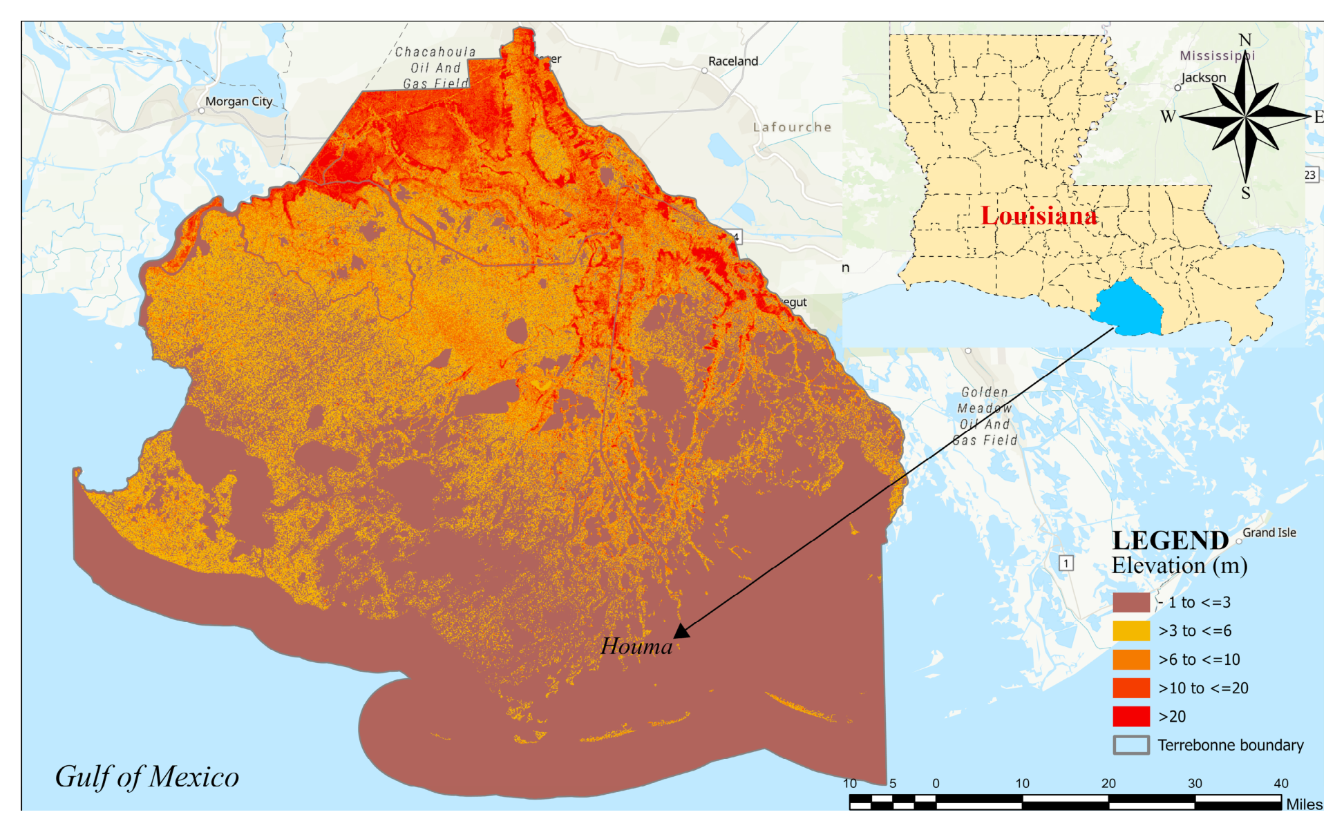
Terrebonne Parish is in the southeastern coastal zone of Louisiana, USA (Figure 1), covering approximately 5500 km². The parish is bounded by the Gulf of Mexico to the south and contains some of the most biologically productive coastal wetlands in North America, supporting commercial fisheries, extensive oil and gas infrastructure, and a population of approximately 110,000 residents concentrated in and around Houma, the parish seat. Terrebonne Parish was selected as the benchmark setting for four reasons. First, it is among the few places on Earth where all four studied hazards are simultaneously and intensely expressed. The parish lies within the Mississippi River deltaic plain, which accounts for the majority of coastal wetland loss in the conterminous United States; it records some of the world’s fastest rates of relative sea-level rise, has sustained repeated major hurricane impacts (Gustav in 2008, Ida in 2021), and is undergoing progressive salinization of its freshwater and intermediate marshes [3,16]. Second, it is geomorphologically archetypal: a low-relief plain of compacting Holocene deltaic sediments, organic marsh soils, and a dense distributary bayou-and-canal network, the same structural template as the world’s other large, inhabited deltas, so a framework validated here transfers conceptually to those settings. Third, the parish offers exceptional data density for evidence-based label construction and validation, effective FEMA flood-zone delineations, long-record USGS gauging and salinity monitoring, NOAA tide gauges, published geodetic subsidence measurements (tide-gauge-derived and GPS), and complete SSURGO soil coverage, prerequisites for the 65-factor predictor stack this framework requires. Fourth, steep north–south hazard gradients within a compact extent make the parish a demanding testbed for spatial evaluation: models must transfer across pronounced environmental transitions over short distances, precisely the conditions under which validation design matters most.

3.2. Topographic and Geomorphic Characteristics

Terrebonne Parish is characterized by extremely low relief typical of the Mississippi River deltaic plain. Elevations range from below sea level in coastal marsh areas to approximately 5–8 m in the northern upland fringe. The landscape is dominated by emergent freshwater, intermediate, brackish, and saline marshes, interspersed with bayous, canals, and shallow bays. The near-zero topographic gradients and extensive hydrological connectivity across the parish are the primary geomorphic controls on flood propagation, storm surge penetration, and salinity intrusion dynamics.

3.3. Climate and Hydrology

The parish experiences a humid subtropical climate (Köppen Cfa; [24]) with hot, humid summers and mild winters. Mean annual precipitation ranges from approximately 1276 to 1707 mm, with a summer maximum associated with convective thunderstorms and tropical cyclones. The hydrological regime is governed by tidal exchange, river discharge, and precipitation-driven sheet flow across low-gradient marsh surfaces.

3.4. Coastal Dynamics and Hazard Context

Tides are microtidal, with National Oceanic and Atmospheric Administration (NOAA) tide gauges recording some of the fastest rates of relative sea-level rise in the world due to combined eustatic rise and regional land subsidence [16]. Geodetic measurements indicate spatially variable subsidence rates, highest in areas of hydrocarbon extraction, Holocene sediment compaction, and organic soil oxidation. Terrebonne is highly exposed to tropical cyclones: Hurricanes Gustav (2008) and Ida (2021) caused severe impacts, with Ida making landfall as a Category 4 storm over the parish. Federal Emergency Management Agency (FEMA) flood zone classifications range from Zone X, which denotes minimal flood hazard outside the 500-year floodplain, to Zone VE, which designates high-risk coastal areas subject to wave action with Base Flood Elevations assigned. The oil and gas sector exerts substantial landscape influence through canal dredging, fluid withdrawal, and associated infrastructure.

Each of the four hazards is individually severe in Terrebonne. Flooding: much of the parish lies within FEMA Special Flood Hazard Areas, and the parish has sustained repeated federally declared flood disasters, with Hurricanes Gustav (2008) and Ida (2021) producing widespread inundation. Land subsidence: measured rates in coastal Louisiana average approximately 9 mm yr⁻¹, among the highest of any populated coastal region, with local maxima associated with hydrocarbon extraction and drained organic soils [16]. Storm surge: the parish’s open, low-gradient shoreline allowed Ida’s Category 4 landfall surge to penetrate far inland, and comparable exposure recurs on decadal timescales. Salinity intrusion: progressive salinization has converted extensive freshwater and intermediate marsh toward brackish and saline states, contributing to the parish’s share of Louisiana’s 4833 km² of coastal land loss since 1932 [3]. No hazard is a minor addition to the composite: all four are individually consequential, which is why the composite index assigns them equal standing, a choice justified, and stress-tested against alternative weightings, in Section 4 and Section 6.5. These processes are tightly interlinked within the parish. Degradation of the Isles Dernieres and Timbalier barrier-island chains has weakened the first line of defense against hurricane surge, allowing storm events to push saline Gulf water through Terrebonne and Timbalier Bays and up the parish’s distributary bayous and navigation canals, most directly the Houma Navigation Canal, deep into interior freshwater marshes [3]. Each surge event thus produces simultaneous flooding and a pulse of salinization; recurrent saltwater exposure stresses flood-attenuating marsh vegetation and accelerates oxidation of the parish’s organic soils, which, together with compaction of Holocene deposits and legacy hydrocarbon extraction, sustains some of the highest subsidence rates on the Louisiana coast [16]. Subsidence in turn deepens flood ponding, extends the inland reach of subsequent surges, and enlarges the tidally influenced zone, while the dense dredged-canal network provides increasingly efficient conduits for salt transport [4]. Hurricane Ida (2021) illustrated this compound behavior concretely, producing surge inundation, extensive wetland loss, and elevated interior-marsh salinity as a single cascading event. The parish is therefore exposed not merely to four hazards but to their interactions, the specific condition the integrated framework of this study is designed to assess.

4. Methodology

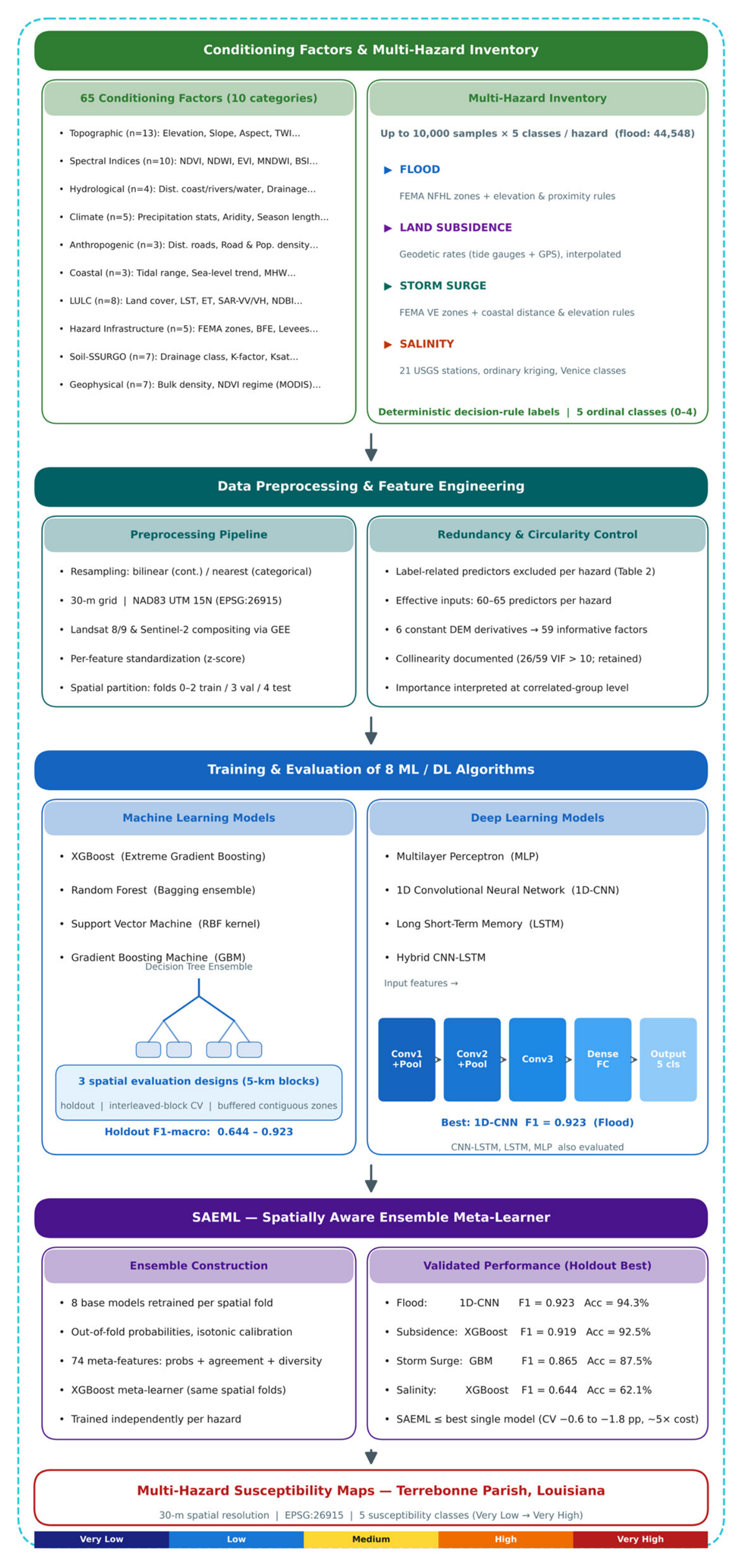
This section presents the complete methodological framework encompassing five principal stages: (1) multi-source conditioning factor compilation and harmonization; (2) hazard label generation and predictor exclusion to prevent circular reasoning; (3) stratified sampling, data partitioning, and preprocessing; (4) training and systematic spatial evaluation of eight ML and DL algorithms alongside the proposed SAEML; and (5) five-class susceptibility map generation and composite index derivation. The overall workflow is summarized in Figure 2.

4.1. Multi-Source Conditioning Factor Dataset

Sixty-five environmental conditioning factors were assembled from remote sensing platforms, in situ networks, government databases, and derived geospatial products (

Table 1. The 65 environmental conditioning factors compiled for multi-hazard susceptibility mapping in Terrebonne Parish, organized by thematic category. GEE = Google Earth Engine; NHD = National Hydrography Dataset; NLCD = National Land Cover Database; SSURGO = Soil Survey Geographic Database; LA = Louisiana; Res. = spatial resolution.

No.	Factor	Category	Source	Res.
1	Aspect	Topographic	30 m DEM derivative	30 m
2	Convergence Index	Topographic	30 m DEM derivative	30 m
3	Elevation	Topographic	USGS 3DEP/SRTM	30 m
4	Hill Shade	Topographic	30 m DEM derivative	30 m
5	Plan Curvature	Topographic	30 m DEM derivative	30 m
6	Profile Curvature	Topographic	30 m DEM derivative	30 m
7	Slope	Topographic	30 m DEM derivative	30 m
8	SPI	Topographic	30 m DEM derivative	30 m
9	Total Curvature	Topographic	30 m DEM derivative	30 m
10	TPI-Large	Topographic	30 m DEM derivative	30 m
11	TPI-Small	Topographic	30 m DEM derivative	30 m
12	TRI	Topographic	30 m DEM derivative	30 m
13	TWI	Topographic	30 m DEM derivative	30 m
14	BSI	Spectral	Sentinel-2/Landsat (GEE)	30 m
15	EVI	Spectral	Sentinel-2/Landsat (GEE)	30 m
16	MNDWI	Spectral	Sentinel-2/Landsat (GEE)	30 m
17	NDBI	Spectral	Sentinel-2/Landsat (GEE)	30 m
18	NDSI	Spectral	Sentinel-2/Landsat (GEE)	30 m
19	NDVI	Spectral	Sentinel-2/Landsat (GEE)	30 m
20	NDWI	Spectral	Sentinel-2/Landsat (GEE)	30 m
21	SAVI	Spectral	Sentinel-2/Landsat (GEE)	30 m
22	SI-1	Spectral	Sentinel-2/Landsat (GEE)	30 m
23	SI-3	Spectral	Sentinel-2/Landsat (GEE)	30 m
24	Dist. to Coastline	Hydrological	NHD/coastline shapefile	30 m
25	Dist. to Rivers	Hydrological	NHD flowlines	30 m
26	Dist. to Waterbodies	Hydrological	NHD waterbodies	30 m
27	Drainage Density	Hydrological	NHD flowlines (derived)	30 m
28	Aridity Index	Climate	PRISM/WorldClim v2	30 m
29	Growing Season Length	Climate	PRISM/NOAA	30 m
30	Max 24 h Precip.	Climate	PRISM	30 m
31	Mean Annual Precip.	Climate	PRISM	30 m
32	Precip. Seasonality	Climate	WorldClim v2	30 m
33	Dist. to Roads	Anthropogenic	TIGER/Line Roads	30 m
34	Population Density	Anthropogenic	LandScan/Census 2020	30 m
35	Road Density	Anthropogenic	TIGER/Line Roads (derived)	30 m
36	Mean High Water	Coastal	NOAA CO-OPS tidal gauges	30 m
37	Sea-Level Trend	Coastal	NOAA CO-OPS tidal gauges	30 m
38	Tidal Range	Coastal	NOAA CO-OPS tidal gauges	30 m
39	Dist. to Urban	LULC	NLCD 2021	30 m
40	Dist. to Wetland	LULC	NLCD 2021	30 m
41	Evapotranspiration	LULC	MODIS MOD16A2	500 m->30 m
42	Land Surface Temp.	LULC	MODIS MOD11A1	1 km->30 m
43	LULC Type	LULC	NLCD 2021	30 m
44	SAR VH	LULC	Sentinel-1 GRD (GEE)	10 m->30 m
45	SAR VV	LULC	Sentinel-1 GRD (GEE)	10 m->30 m
46	Water Occurrence	LULC	JRC Global Surface Water	30 m
47	Base Flood Elevation	Hazard Infra.	FEMA FIRM/BFE grid	30 m
48	Canal Density	Hazard Infra.	LA hydrography layer	30 m
49	Dist. to Levee	Hazard Infra.	USACE/CPRA levee data	30 m
50	FEMA Flood Zone	Hazard Infra.	FEMA FIRM (2023)	30 m
51	Oil/Gas Well Density	Hazard Infra.	Louisiana DNR well registry	30 m
52	Bulk Density	Geophysical	POLARIS soil dataset	30 m
53	NDVI Long-Term Mean (MODIS)	Geophysical	MODIS MOD13A3	1 km->30 m
54	NDVI Seasonal Variability (MODIS)	Geophysical	MODIS MOD13A3 (derived)	30 m
55	NDWI Seasonal Variability (MODIS)	Geophysical	Sentinel-2/Landsat (GEE)	30 m
56	Relative Elevation	Geophysical	DEM/NHD (derived)	30 m
57	Soil Erodibility (K)	Geophysical	USDA SSURGO	30 m
58	Subsidence Rate	Geophysical	Geodetic (NOAA tide-gauge trend + published GPS)	30 m
59	SSURGO Drain. Class	Soil	USDA SSURGO (2023)	30 m
60	SSURGO Flood Freq.	Soil	USDA SSURGO (2023)	30 m
61	SSURGO Hydro. Group	Soil	USDA SSURGO (2023)	30 m
62	SSURGO Ksat	Soil	USDA SSURGO (2023)	30 m
63	SSURGO Organic Matter	Soil	USDA SSURGO (2023)	30 m
64	SSURGO Pond Freq.	Soil	USDA SSURGO (2023)	30 m
65	SSURGO Water Table	Soil	USDA SSURGO (2023)	30 m

). All factors were resampled to 30 m resolution and projected to NAD83 UTM Zone 15N (EPSG:26915), organized into ten thematic categories.

Each thematic category corresponds to physical control on one or more of the four hazards, and the stack was designed for process coverage rather than variable count. Topographic factors govern gravitational water routing and ponding (flood), surge run-up extent, and relative exposure to inundation as the land surface subsides. Spectral indices provide current-condition proxies for vegetation vigor, surface moisture, and surface salinity expression, which modulate infiltration, evapotranspiration, and marsh integrity. Hydrological distance factors encode proximity to the conveyance network through which floodwater, surge, and salt propagate. Climate factors capture the precipitation regime that drives pluvial flooding and the freshwater balance that opposes salinity intrusion. Anthropogenic factors register development pressure and impervious surfaces that alter runoff and exposure. Coastal factors, tidal range, Sea-Level Trend, and mean high water set the marine boundary conditions for surge and salinity intrusion. Land use/land cover factors describe surface roughness, wetland buffering capacity, and the thermal–hydrological regime of the surface. Hazard-infrastructure factors represent both engineered protection and engineered drivers: levees and Base Flood Elevations encode designed defenses, while dredged canals accelerate salt transport and wetland fragmentation, and hydrocarbon extraction contributes to subsidence. Soil factors control infiltration, drainage, compressibility, and organic-matter content, the primary substrate controls on subsidence and flood retention. Geophysical factors capture subsurface compaction potential and hydro-ecological seasonality. Within each category, a variable was retained when it (i) had a defensible mechanistic link to at least one hazard, (ii) was available wall-to-wall at or near the 30 m analysis grid, and (iii) originated from an authoritative, documented source. Redundancy among correlated variables was deliberately accepted at the compilation stage and is quantified explicitly in Section 4.2, leaving the tree-based and deep learners to weight correlated evidence.

Using one shared stack for all four hazards, rather than four bespoke compilations, is likewise a deliberate design choice. First, commensurability: the composite index is defensible only if the four susceptibility surfaces derive from identical inputs, resolution, and preprocessing; hazard-specific stacks would confound differences between hazards with differences between datasets. Second, relevance is enforced where it is critical: variables involved in constructing a hazard’s labels are excluded from that hazard’s predictor set (

Table 2. Feature exclusion per hazard to prevent circular reasoning in susceptibility modeling.

Hazard	Total	Included	Excluded (n)	Excluded Features
Flood	65	60	5	Elevation, TWI, Dist. to Rivers, Dist. to Waterbodies, FEMA Flood Zone
Subsidence	65	64	1	Subsidence Rate
Storm Surge	65	62	3	Elevation, Dist. to Coastline, FEMA Flood Zone
Salinity	65	65	0	None (labels from USGS water quality monitoring)

), so the effective input differs by hazard (60 predictors for flood, 62 for storm surge, 64 for subsidence, 65 for salinity). Third, low-relevance factors are empirically self-pruning: permutation importance shows that the 30 least influential predictors jointly carry approximately 2% of total importance in the salinity models, with mechanistically remote factors such as road density ranking 46th of 65 at roughly 1% of the leading predictor’s importance, the algorithms assign such factors negligible weight rather than being misled by them. The per-hazard importance rankings (Section 5.5) therefore double as an empirical relevance screen, documenting which of the shared factors each hazard’s models use.

Harmonization to the 30 m analysis grid followed data-type-specific rules chosen to minimize resampling artifacts. Continuous rasters, MODIS land surface temperature and evapotranspiration, SoilGrids bulk density, MODIS NDVI, Sentinel-1 backscatter, and the coarse-resolution climate surfaces were resampled by bilinear interpolation, whereas categorical and class-coded layers, land cover, FEMA flood zones, water occurrence, and SSURGO soil attributes were assigned by nearest-neighbor or rasterized directly from source polygons, which preserves class codes and introduces no synthetic values. Sentinel-2-derived indices were composited and exported at the 30 m analysis scale in Google Earth Engine. Two forms of uncertainty follow, and they behave differently. For coarse-native datasets (500 m to 4 km), resampling to 30 m creates no information at 30 m: these variables act as smooth regional fields whose effective resolution remains their native one, appropriate for the broad-scale drivers they represent (climate regime, geophysical setting), but incapable of resolving local variation, a constraint noted in the Limitations. For fine-native datasets (10 m Sentinel-2), aggregation entails minor smoothing of sub-grid detail. Residual resampling uncertainty nonetheless propagates into the predictor stack, and is a further reason redundancy across thematic groups (Section 4.2) was tolerated: correlated evidence from independent sources buffers single-layer error. The native resolution of every dataset is documented in Table 1.

The datasets span acquisition periods matched to the processes they represent, and Table 1 lists the acquisition year(s) of every source. Static or slowly varying properties, SRTM topography (February 2000), SSURGO soil attributes, and geophysical setting are treated as time-invariant at the decadal scale of susceptibility assessment. Current-condition variables describe the contemporary landscape state: Sentinel-2 annual and seasonal composites, Landsat 8/9 composite, and Sentinel-1 backscatter statistics (cloud-free multi-temporal composites assembled in Google Earth Engine at factor compilation, January–February 2026), NLCD 2021, and the effective FEMA NFHL and SSURGO releases (accessed January 2026). Long-term regime variables deliberately integrate multi-year records: PRISM/ACIS climate statistics (2000–2023), WorldClim v2 normals (1970–2000), MODIS-derived vegetation and water regime metrics (multi-year record through compilation), JRC surface-water occurrence (1984 onward), NOAA tidal statistics and Sea-Level Trends (full station periods of record), USGS salinity records (2000–2024), and geodetic subsidence rates from tide-gauge trends and published GPS campaigns. This temporal mixture is by design: susceptibility is a quasi-static property driven jointly by the current landscape state and the long-term process regime, regime variables require multi-decadal averaging to be stable, while state variables must be recent. The consequence is that predictors and labels align at the regime level, and the resulting maps represent susceptibility under the contemporary landscape configuration and recent climate, consistent with the static scope acknowledged in the Limitations.

Topographic Factors (13): Derived from a 30 m DEM: aspect, convergence index, elevation, hillshade, plan curvature, profile curvature, slope, Stream Power Index (SPI), total curvature, TPI-large (15-cell), TPI-small (3-cell), Terrain Ruggedness Index (TRI), and Topographic Wetness Index (TWI).

Spectral Indices (10): Calculated from annual composites of Sentinel-2 and Landsat imagery via Google Earth Engine [25,26]: Bare Soil Index (BSI), Enhanced Vegetation Index (EVI), Modified Normalized Difference Water Index (MNDWI), Normalized Difference Built-up Index (NDBI), Normalized Difference Salinity Index (NDSI), Normalized Difference Vegetation Index (NDVI), Normalized Difference Water Index (NDWI), Soil-Adjusted Vegetation Index (SAVI), Salinity Index-1 (SI-1), and Salinity Index-3 (SI-3).

Hydrological Factors (4): Distance to coastline, rivers, waterbodies, and drainage density.

Climate Factors (5): Aridity index, growing season length, maximum 24 h precipitation, mean annual precipitation, and precipitation seasonality from PRISM [27] and WorldClim v2 [28].

Anthropogenic Factors (3): Distance to roadways, population density, and road density.

Coastal Factors (3): Mean high water level, Sea-Level Trend, and tidal range from NOAA CO-OPS tidal station records [29].

Land Use/Land Cover Factors (8): Distance to urban, distance to wetlands, evapotranspiration (ET), land surface temperature (LST), LULC classification from NLCD 2021 [30], Sentinel-1 SAR backscatter (VH, VV polarizations), and JRC Global Surface Water occurrence [31].

Hazard Infrastructure Factors (5): Base Flood Elevation (BFE), canal density, distance to levee, FEMA flood zone classification [32], and oil/gas well density.

Soil Factors (7): From USDA SSURGO [33]: drainage class, flood frequency rating, hydrologic soil group, saturated hydraulic conductivity (Ksat), organic matter content, ponding frequency, and depth to seasonal high-water table.

Geophysical Factors (7): Bulk density, MODIS NDVI [34], NDVI seasonal variation, NDWI seasonal variation, relative elevation (height above nearest drainage), soil erodibility (K-factor), and subsidence rate from geodetic measurements. Note that the spectral category’s NDVI and the geophysical category’s MODIS-derived NDVI variables are distinct rather than duplicated: the former is a 30 m annual composite from Sentinel-2/Landsat representing current fine-scale vegetation condition, whereas the latter, labeled “NDVI long-term mean (MODIS)” and “NDVI seasonal variability (MODIS)”, derive from the multi-year 1 km MODIS record and characterize the vegetation regime. The two NDVI variables correlate at only r = 0.33 across the study area, confirming complementary rather than redundant information.

Quality screening of the compiled stack revealed that six DEM-derived variables, plan curvature, profile curvature, total curvature, TPI-large, TPI-small, and TRI, are constant (zero) across the study area, a consequence of computing curvature-type derivatives from an integer-meter DEM over terrain with near-zero relief. These variables were retained in the stack for completeness but carry no information; the effective predictor count is therefore 59. Their presence does not affect model training, as constant features receive zero splits and zero importance.

4.2. Multicollinearity and Predictor Redundancy

Multicollinearity among the predictors was assessed through pairwise Pearson correlation and variance inflation factors (VIF), reported in full as Supplementary Figure S1 and Table S1. As expected for a comprehensive environmental stack, redundancy is substantial: the vegetation-index family is nearly collinear (NDVI/SAVI/EVI pairwise |r| = 0.95–1.00), 81 predictor pairs exhibit |r| ≥ 0.8, and 26 of the 59 informative predictors exceed the conventional VIF threshold of 10, led by the spectral water and salinity indices. Redundant predictors were retained rather than removed, for two reasons: tree-based ensembles and regularized neural networks are robust to predictor redundancy for prediction, and removal risks discarding hazard-specific information in a stack shared across four physically distinct hazards. The interpretive consequence, that permutation importance can be shared or diluted among correlated predictors, is acknowledged in the feature-importance methodology and Discussion, and importance rankings are interpreted at the level of correlated factor groups where appropriate.

4.3. Hazard Label Generation and Feature Exclusion

Susceptibility labels for each hazard were generated by transparent, deterministic decision rules applied to authoritative evidence layers and classified into five ordinal classes: Very Low (0), Low (1), Moderate (2), High (3), and Very High (4). No numerical weighting was used: each pixel was assigned according to the first matching rule in the fixed hierarchies below, which are stated in full to ensure reproducibility.

Flood: Labels derive from FEMA National Flood Hazard Layer (NFHL) effective flood zones augmented with topographic and hydrographic criteria: Zone VE → Very High; Zones A/AE (and equivalent A-type zones) → High; Zone X with elevation < 3 m and distance to rivers < 2 km, or unmapped areas with elevation < 2 m and distance to waterbodies < 1 km → Moderate; remaining Zone X areas, and areas with elevation < 5 m and Topographic Wetness Index > 5 → Low; all remaining areas → Very Low.

Land subsidence: The subsidence-rate surface, interpolated by thin-plate spline from 25 geodetic observations (11 NOAA tide-gauge-derived rates with the global mean Sea-Level Trend removed, and 14 published GPS and geodetic measurements; [35,36,37]), was classified by rate thresholds: <2 (Very Low), 2–5 (Low), 5–8 (Moderate), 8–11 (High), and ≥11 mm yr⁻¹ (Very High).

Storm surge: FEMA VE coastal velocity zones → Very High; outside Zone VE, susceptibility was assigned by joint coastal-proximity and elevation criteria: distance to coastline < 5 km and elevation < 3 m → High; distance < 15 km and elevation < 5 m → Moderate; distance < 30 km and elevation < 8 m → Low; otherwise Very Low.

Salinity intrusion: Mean specific conductance for 2000–2024 was compiled for 21 USGS NWIS monitoring stations across Terrebonne, Lafourche, and Plaquemines Parishes and converted to salinity (PSU) via the PSS-78 relation. Station salinities were interpolated to the 30 m grid by ordinary kriging (exponential variogram fitted to the real stations only; effective range ≈ 168 km), with a marine boundary condition of eight pseudo-stations at 35 PSU along the open-Gulf edge of the domain, required because kriging cannot exceed its data range, and the estuarine station network (maximum 29.3 PSU) would otherwise misclassify the open Gulf. The kriging variance surface is provided as a spatial map of label confidence (Supplementary Figure S2), and leave-one-station-out cross-validation yields RMSE = 3.40 PSU (12% of the observed range), bias = +0.59 PSU, and R² = 0.82, with correct class assignment at 12 of 21 stations. The kriged surface was classified by Venice System thresholds: <0.5 (Very Low), 0.5–5 (Low), 5–18 (Moderate), 18–30 (High), >30 PSU (Very High). The spectral salinity indices (NDSI, SI-1, SI-3) are conditioning factors only and played no role in label generation. To prevent circular reasoning, a methodological pitfall whereby variables used to construct hazard labels are also used as predictors, artificially inflating model performance features directly involved in label generation were systematically identified and excluded from each hazard’s predictor set (Table 2). This exclusion is essential for generating genuine predictive relationships rather than tautological label reconstruction.

4.4. Sampling Strategy and Data Partitioning

To ensure class balance and geographic coverage, up to 10,000 pixels per susceptibility class were randomly sampled per hazard from all valid pixels (50,000 samples for subsidence, storm surge, and salinity; 44,548 for flood, where the Very Low class is exhausted at 4548 available pixels). Without balancing, naturally imbalanced class distributions bias classifiers toward dominant classes. Data partitioning is spatial rather than random: the study area was tessellated into 5 km × 5 km blocks, blocks were assigned to five folds by seeded random interleaving, and folds 0–2 (≈60%) served as the training set, fold 3 (≈20%) as the validation set for hyperparameter selection and early stopping, and fold 4 (≈20%) as the holdout test set, which was never exposed to any model-selection procedure. The holdout evaluation is therefore itself spatially blocked at the 5 km scale, a property whose consequences for interpreting holdout-versus-cross-validation comparisons are analyzed in Section 5.4.

This balanced design has three implications for calibration and real-world use. First, predicted class probabilities are calibrated to the balanced training distribution rather than to true areal prevalence; raw probabilities should not be read as real-world class frequencies, although prevalence re-weighting is a straightforward post-processing correction. Second, the final susceptibility maps are discrete class assignments, which are far less sensitive to prevalence shift than probability magnitudes. Third, all eight algorithms were faced with the identical sampling design, so the comparative conclusions, which algorithm transfers best, and by how much, are unaffected by the balancing choice.

4.5. Machine Learning Algorithms

The eight algorithms were selected to span four complementary learning mechanisms within each of the ML and DL families, rather than to maximize the number of models compared. Among the ML methods, RF represents bagging with variance reduction through randomized ensembles, XGBoost and GBM represent two contrasting implementations of gradient boosting (regularized second-order optimization versus classical sequential correction), and SVM represents kernel-based maximum-margin learning, collectively the mechanisms that dominate the susceptibility-mapping literature [7,12]. Among the DL methods, MLP represents fully connected universal approximation, 1D-CNN local cross-feature interaction extraction, LSTM gated sequential memory, and CNN-LSTM a stacked convolutional–recurrent representation; the architecture families most frequently adapted to tabular geospatial inputs [8,14]. Three practical criteria further constrained the selection: documented performance in prior hazard susceptibility applications, computational feasibility at the 50,000-sample scale of this study on CPU workstation hardware, and availability of directly comparable implementations under an identical training protocol. The deliberate retention of LSTM, despite published doubts about its suitability for unordered tabular data [7], provides a direct empirical test of that concern. Hyperparameters for all eight models were selected through systematic grid-search cross-validation on the held-out validation partition (fold 3; Section 4.4), with the search conducted independently for each algorithm–hazard combination prior to final evaluation on the holdout test set. Final configurations are reported below.

XGBoost: Regularized gradient boosting ensemble with parameters: max_depth = 8, learning_rate = 0.1, n_estimators = 300, subsample = 0.8, colsample_bytree = 0.8 [13].

Random Forest (RF): Bagging ensemble with bootstrap sampling and random feature subsets: n_estimators = 300, max_depth = 20, min_samples_split = 5, min_samples_leaf = 2,

max_features = sqrt(n) [19].

SVM: RBF kernel with C = 10, gamma = ‘scale’; features standardized to zero mean and unit variance prior to training [21].

GBM: Sequential gradient correction: n_estimators = 200, max_depth = 6, learning_rate = 0.1, subsample = 0.8, min_samples_split = 5 [20].

4.6. Deep Learning Architectures

MLP: Three hidden layers (256-128-64 neurons), ReLU activation, batch normalization, dropout (0.3). Implemented via scikit-learn MLPClassifier with Adam optimizer and early stopping [38].

1D-CNN: Two convolutional layers (64/128 filters, kernel size 3), ReLU, batch norm, adaptive average pooling, fully connected layers (2048-128-n_classes), dropout (0.3). PyTorch implementation, 50 epochs with early stopping [8].

LSTM: Two-layer gated memory cell network (128 hidden units, dropout 0.3), two fully connected layers (64-n_classes). Adam optimizer with early stopping [22].

CNN-LSTM: Two convolutional layers (64 filters, kernel 3) with batch norm and ReLU, followed by LSTM layer (128 units), two fully connected layers (64-n_classes), dropout (0.3) [15].

To diagnose overfitting risk at this sample size, training- and validation-accuracy learning curves were computed for all four DL architectures on every hazard as a function of training-set fraction (Supplementary Figure S4). The curves show the canonical converging pattern rather than divergence: validation accuracy rises monotonically with training-set size while the train–validation gap narrows, indicating that the 30-epoch early-stopping protocol (validation-based checkpoint selection, patience of 10) controls overfitting and that the models operate in a data-sufficient regime at approximately 30,000–35,000 effective training samples. Two architecture-specific observations follow. The sequence models (LSTM, CNN-LSTM) converge more slowly and erratically than the 1D-CNN and MLP, consistent with their optimization overhead on non-sequential inputs (Section 6.1) but likewise show no runaway train–validation divergence. More importantly, the learning curves bound only the classical, sample-size form of generalization error; the decisive risk in this setting is spatial generalization, which no within-distribution diagnostic can detect and which the three-design spatial evaluation (Section 5.4) quantifies directly: a model can be perfectly well-fit in the learning-curve sense and still degrade sharply under buffered contiguous-zone evaluation.

4.7. Spatial Evaluation Designs

Model generalizability was assessed under three progressively stricter spatial designs. (1) Spatially blocked holdout: the fold-four test set described above. (2) Interleaved-block cross-validation: five-fold cross-validation over the same 5 km blocks, with blocks assigned to folds by seeded random interleaving; in each iteration four folds are used for training and one for testing. Because neighboring blocks generally belong to different folds, training and test samples can lie within tens of meters of one another across block boundaries; this design controls for block-scale heterogeneity but not for short-range spatial dependence. (3) Strict contiguous-zone cross-validation: the blocks were grouped into five geographically contiguous west-to-east zones balanced by sample count, and in each iteration all training samples within 5 km of any test sample were additionally discarded, guaranteeing a minimum 5 km separation between training and test data.

The 5 km scale is supported by empirical variograms of representative conditioning factors (Supplementary Figure S3): fitted effective ranges span 22–150 km (median ≈ 31 km), reflecting the regional gradients that dominate deltaic environmental structure, but the variograms are strongly structured at short range, with roughly half of the total semivariance accruing within the first 5 km. The 5 km buffer of the strict design therefore removes the steep short-range dependence. At the same time, the residual long-range structure cannot be blocked out within a single parish, which is precisely why comparing the three designs is informative: their divergence measures how much apparent skill each level of spatial control leaves in place.

4.8. Performance Metrics

Model performance was assessed using: overall accuracy (OA), F1-macro (unweighted mean of per-class F1 scores, selected as the primary metric for its equal treatment of all classes), F1-weighted (frequency-weighted F1), Cohen’s Kappa (k) [39], Precision-macro, Recall-macro, and per-class F1 scores for all five susceptibility classes.

4.9. Permutation-Based Feature Importance

Permutation-based feature importance was computed for XGBoost, RF, and GBM following the algorithm of Breiman [19]. For each predictor in turn, its values were randomly permuted on the holdout test set while all other predictors remained unchanged, and the resulting decrease in F1-macro relative to the unpermuted baseline was recorded as the feature’s importance score. This procedure was repeated five times per feature with different random seeds to reduce estimation variance, and mean scores were recorded. Importance scores were subsequently averaged across the three tree-based models to produce a model-averaged, algorithm-robust assessment that is less sensitive to the idiosyncratic feature preferences of any single algorithm. Permutation importance was not computed for SVM, MLP, 1D-CNN, LSTM, or CNN-LSTM given the substantially greater computational cost for these architectures and their lack of inherent feature attribution mechanisms. Permutation importance quantifies each predictor’s contribution to model predictions: it identifies statistical association, not causal influence, and importance can be shared or diluted among correlated predictors (Section 4.2). Rankings are therefore interpreted as statistically grounded hypotheses about process, to be corroborated against independent physical evidence, rather than as causal attribution.

4.10. Susceptibility Map Generation

Final susceptibility maps were generated by applying XGBoost, trained per hazard on its full training partition, to the complete Terrebonne Parish raster stack (9,266,642 pixels at 30 m resolution) using a memory-efficient chunk-based prediction pipeline. XGBoost was used for map production across all four hazards, rather than the per-hazard holdout leader, for three reasons. First, performance: XGBoost is the top holdout performer for land subsidence (F1-macro = 0.919) and salinity intrusion (0.644), and within 0.017 and 0.003 F1-macro of the leaders for flood (0.906 versus 0.923, 1D-CNN) and storm surge (0.862 versus 0.865, GBM), respectively. Second, consistency: a single algorithm family yields class-probability surfaces with uniform calibration behavior across the four hazards, which matters when the surfaces are combined into a composite index. Third, practicality: seconds-scale training and efficient batched prediction make parish-scale map regeneration computationally trivial, supporting the operational updating envisioned in Section 6.5. Both five-class classification maps and continuous probability maps were generated per hazard.

The composite Multi-Hazard Susceptibility Index (MHSI) was computed as the arithmetic mean of normalized class values (class/4) across the four hazards. Equal weighting was adopted because hazard severity is application-dependent, salinity intrusion dominates threats to freshwater supply while storm surge dominates threats to structures, so no application-independent differential weighting can be defended a priori; equal weighting is the transparent, assumption-minimal baseline of composite-indicator practice, and all four individual surfaces are published for users requiring application-specific weights. Because 31.9% of the administrative extent is open water, the MHSI is reported in two forms: parish-wide over all valid pixels, and land-masked with open water excluded, the latter recommended for management prioritization, since risk-reduction decisions apply on land. A weighting sensitivity analysis (Section 6.5; Supplementary Table S2) shows that on land, up-weighting any single hazard twofold preserves the top-decile priority zone at 88–94% overlap (Jaccard) with rank correlations of 0.91–0.92 against the equal-weight index; an aggressive surge/flood-dominant scheme relocates the top decile and marks the boundary of this robustness.

4.11. Spatially Aware Ensemble Meta-Learner (SAEML)

The Spatially Aware Ensemble Meta-Learner (SAEML) combines calibrated predictions from all eight base models through a three-stage framework explicitly designed to eliminate spatial data leakage. Unlike conventional stacking which generates base-model predictions on the training set without spatial separation, every component of the SAEML pipeline is conditioned on spatially disjoint partitions, ensuring that the meta-learner never trains predictions from spatially proximal samples. This design eliminates autocorrelation exploitation in the meta-model, but it also constrains the SAEML to learn from a restricted pool of out-of-fold (OOF) predictions; whether this constraint allows the meta-model to exceed the performance of the strongest individual base model is an empirical question addressed in Section 5.7.

Stage 1 Out-of-Fold Prediction Generation: All eight base models were retrained on each of the five spatial folds, generating OOF probability predictions for every training sample from a fold in which that sample was excluded from model training. This produces 40 spatially isolated base models per hazard (8 algorithms × 5 folds), and 160 models in total across all four hazards. Because each OOF prediction is generated by a model that has never seen the sample or its spatial neighbors during training, the complete OOF prediction set constitutes a spatially honest, cross-validated representation of each base model’s behavior at genuinely new locations.

Stage 2 Isotonic Calibration and Meta-Feature Engineering: Raw OOF class probability estimates from each base model were calibrated using isotonic regression, which corrects systematic overconfidence or underconfidence in predicted probabilities without introducing parametric assumptions. The calibrated predictions were then transformed into a 74-dimensional meta-feature matrix with the following explicit structure: 40 calibrated class probability scores (8 models × 5 classes); eight model confidence scores (maximum predicted probability per model); eight predicted class labels encoded as ordinal features. To these were added five per-class prediction variance scores across models; one inter-model agreement entropy score; seven pairwise model disagreement metrics (derived from the four tree-model pairs most likely to disagree); and five softmax margin features capturing class separation confidence (40 + 8 + 8 + 5 + 1 + 7 + 5 = 74). This meta-feature representation provides the meta-learner access to both individual model confidence estimates and inter-model agreement signals.

Stage 3 XGBoost Meta-Learner: An XGBoost classifier was trained on the 74-dimensional meta-feature matrix using the same five spatial folds to maintain consistent spatial separation throughout. Hyperparameters were optimized on the spatial validation folds (max_depth = 4, learning_rate = 0.05, n_estimators = 200, subsample = 0.8). The trained meta-learner was evaluated on the independent holdout test set and additionally through five-fold spatial CV to quantify its holdout-to-CV performance gap, defined as the absolute difference in F1-macro between the holdout test set and spatial cross-validation performance, which serves as the primary metric for diagnosing spatial overfitting.

4.12. Computational Environment

All experiments were conducted on a single workstation (Dell Precision 3680; Intel Core i9-14900, 24 cores/32 threads; 128 GB RAM; Windows 11). All model training and inference used the CPU only; no GPU acceleration was employed. The software environment comprised Python 3.12.10 with scikit-learn 1.8.0, XGBoost 3.2.0, PyTorch 2.10.0 (CPU build), NumPy 2.4.2, pandas 3.0.0, and rasterio 1.5.0. Training the 32 final model–hazard combinations required 71 min in total, with individual models ranging from ~1 s (Random Forest) to ~560 s (LSTM) per hazard (Section 5.3). The SAEML ensemble evaluation (Section 5.7) added a further ≈6.2 h of training. Retraining all eight base models under the interleaved-block and strict contiguous-zone spatial cross-validation designs (Section 5.4) required substantially more compute: the strict design alone totaled approximately 26 h across 320 model–fold combinations, with the slowest individual fold (SVM, storm surge) requiring close to 12 h. The full evaluation was therefore completed over several days rather than in a single run; nonetheless, no specialized computing infrastructure beyond the workstation described above was required at any stage. That the full framework runs on a standard engineering workstation without GPU support underscores its accessibility for operational coastal-management agencies.

5. Results

5.1. Test Set Performance

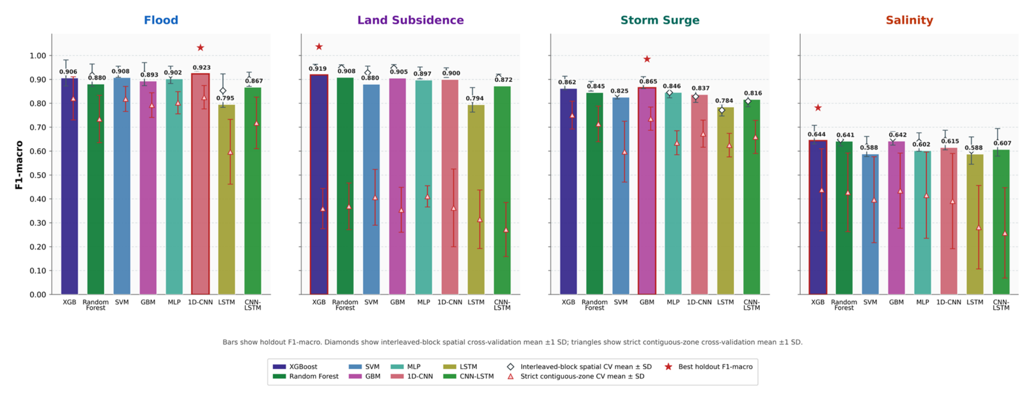
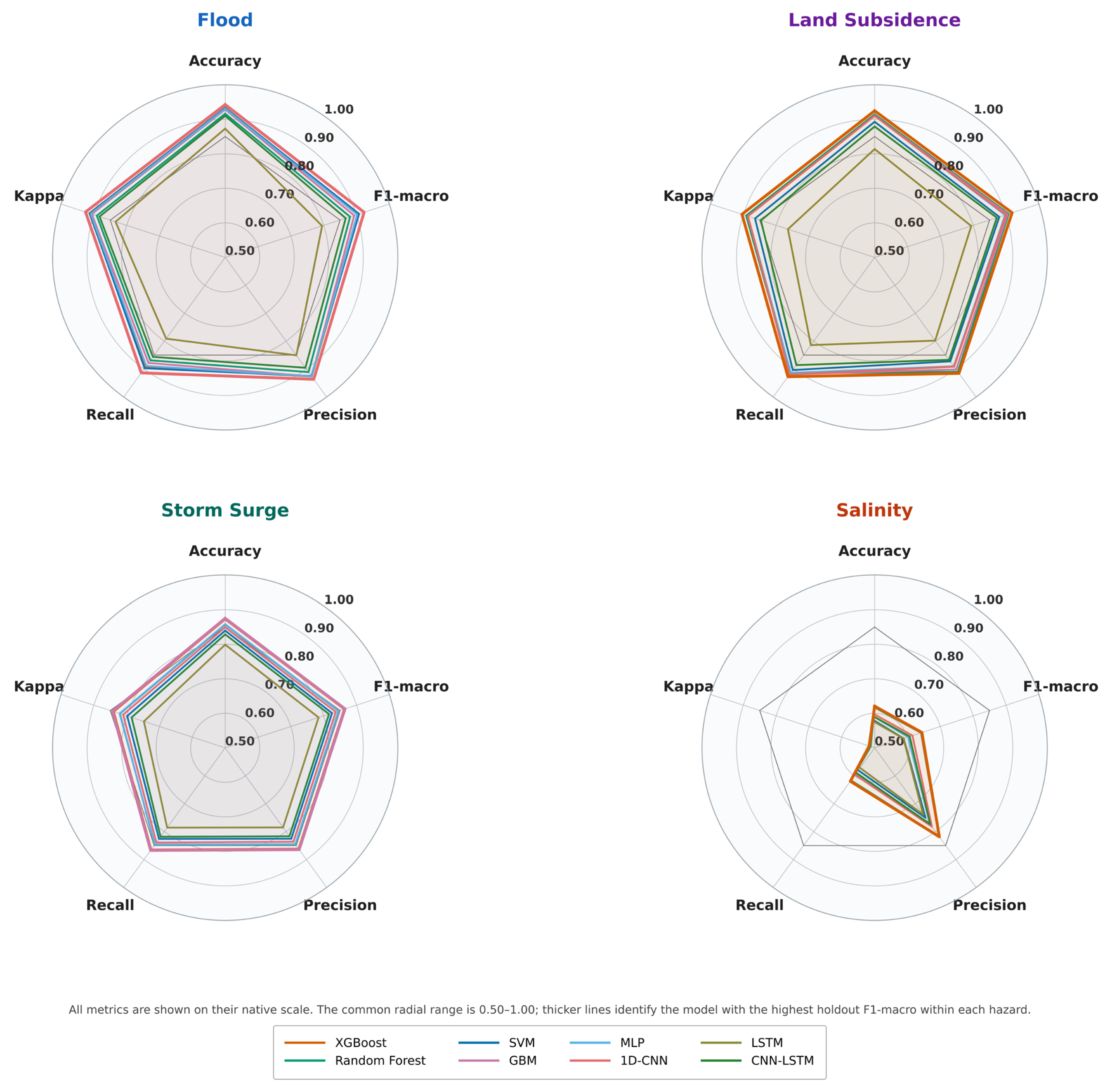
Across the 32 model–hazard combinations evaluated on the independent holdout test set, overall accuracy ranged from 57.5% (LSTM, salinity) to 94.3% (1D-CNN, flood), and F1-macro from 0.588 (LSTM, salinity) to 0.923 (1D-CNN, flood;

Table 3. Complete holdout test performance for all 32 base models (Terrebonne Parish), evaluated on the spatially blocked fold-four holdout partition. * = best model per hazard based on F1-macro. n = number of conditioning factors after per-hazard feature exclusion (Table 2). Time = training time on the CPU workstation described in the Computational Environment subsection.

Hazard	Model	n	Acc.	F1-Macro	F1-wt	Kappa	Time (s)
Flood	XGBoost	60	0.9337	0.9058	0.9323	0.9134	5.5
Flood	Random Forest	60	0.9164	0.8804	0.9159	0.8910	1.4
Flood	SVM	60	0.9330	0.9076	0.9320	0.9126	35.3
Flood	GBM	60	0.9283	0.8930	0.9259	0.9062	195.6
Flood	MLP	60	0.9309	0.9022	0.9293	0.9097	10.4
Flood	1D-CNN *	60	0.9427	0.9232	0.9424	0.9254	69.3
Flood	LSTM	60	0.8730	0.7952	0.8646	0.8340	465.1
Flood	CNN-LSTM	60	0.9101	0.8671	0.9075	0.8827	153.5
Subsidence	XGBoost *	64	0.9247	0.9186	0.9247	0.9041	3.2
Subsidence	Random Forest	64	0.9145	0.9083	0.9146	0.8913	1.2
Subsidence	SVM	64	0.8928	0.8796	0.8936	0.8644	20.4
Subsidence	GBM	64	0.9107	0.9053	0.9102	0.8865	241.6
Subsidence	MLP	64	0.9100	0.8972	0.9105	0.8857	12.1
Subsidence	1D-CNN	64	0.9100	0.8996	0.9099	0.8858	114.1
Subsidence	LSTM	64	0.8138	0.7942	0.8132	0.7642	557.2
Subsidence	CNN-LSTM	64	0.8791	0.8720	0.8774	0.8464	198.1
Storm Surge	XGBoost	62	0.8720	0.8620	0.8728	0.8392	4.0
Storm Surge	Random Forest	62	0.8572	0.8450	0.8574	0.8206	1.3
Storm Surge	SVM	62	0.8395	0.8254	0.8402	0.7983	48.9
Storm Surge	GBM *	62	0.8752	0.8650	0.8754	0.8432	255.3
Storm Surge	MLP	62	0.8582	0.8455	0.8583	0.8216	8.3
Storm Surge	1D-CNN	62	0.8493	0.8368	0.8505	0.8108	106.1
Storm Surge	LSTM	62	0.7990	0.7845	0.8012	0.7476	558.2
Storm Surge	CNN-LSTM	62	0.8286	0.8162	0.8310	0.7850	205.2
Salinity	XGBoost *	65	0.6206	0.6439	0.6296	0.5167	2.4
Salinity	Random Forest	65	0.6171	0.6411	0.6266	0.5123	1.0
Salinity	SVM	65	0.5781	0.5882	0.5732	0.4642	104.8
Salinity	GBM	65	0.6196	0.6418	0.6279	0.5153	168.2
Salinity	MLP	65	0.5890	0.6017	0.5860	0.4780	9.1
Salinity	1D-CNN	65	0.5968	0.6150	0.6014	0.4868	84.1
Salinity	LSTM	65	0.5746	0.5876	0.5770	0.4584	362.7
Salinity	CNN-LSTM	65	0.5892	0.6067	0.5930	0.4775	255.1

, Figure 3). No single algorithm consistently dominated across all four hazards: 1D-CNN achieved the highest F1-macro for flooding (0.923; Acc = 94.3%), XGBoost for land subsidence (0.919; Acc = 92.5%), and GBM for storm surge (0.865; Acc = 87.5%) and XGBoost for salinity intrusion (0.644; Acc = 62.1%). This hazard-dependent ranking replicates the well-documented context-dependence of algorithm performance and extends it to a simultaneous multi-hazard coastal setting. The performance metric radar chart (Figure 4) confirms that top-performing models achieve near-balanced profiles across Accuracy, F1-macro, Precision, Recall, and Cohen’s Kappa, while LSTM displays a noticeably smaller polygon indicating uniformly lower performance across all metrics and hazards, attributable to the architectural mismatch between sequential modeling and unordered tabular inputs. Cohen’s Kappa exceeded 0.88 for all best models except salinity (0.737), confirming strong agreement beyond chance. Overall accuracy and F1-macro were highly concordant (Pearson r = 0.997), validating F1-macro as the primary ranking criterion for the class-balanced experimental design employed here.

5.2. Per-Class Performance and Discrimination

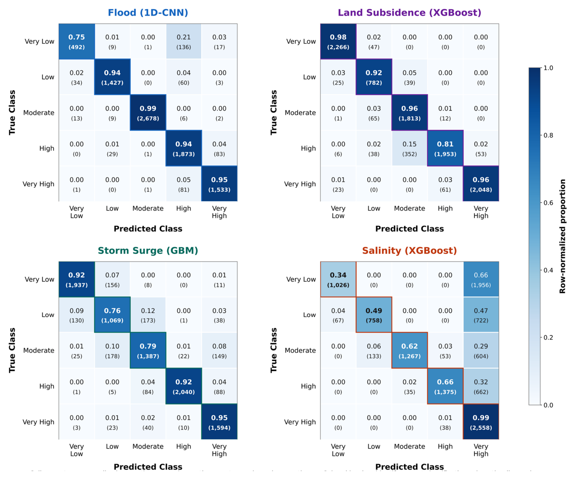
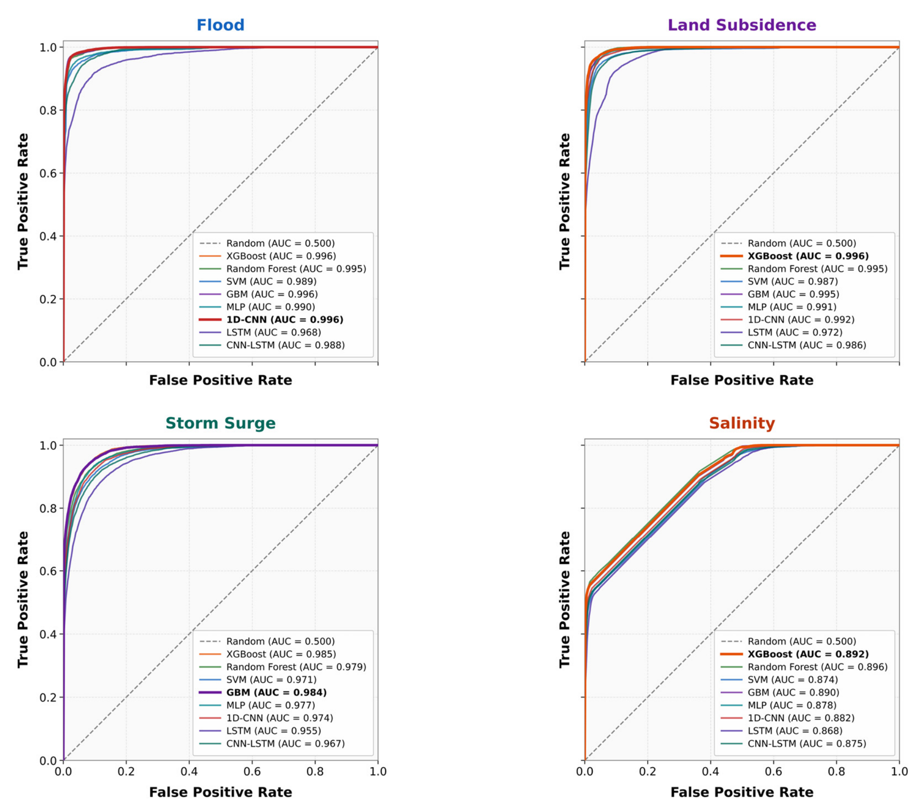
Normalized confusion matrices for the best-performing model per hazard (Figure 5) and per-class F1 scores (

Table 4. Per-class F1 scores for the best-performing model per hazard (Terrebonne Parish).

Hazard	Best Model	F1 (V. Low)	F1 (Low)	F1 (Mod.)	F1 (High)	F1 (V. High)
Flood	1D-CNN	0.823	0.952	0.994	0.904	0.942
Subsidence	XGBoost	0.978	0.880	0.885	0.882	0.968
Storm Surge	GBM	0.921	0.752	0.803	0.951	0.898
Salinity	XGBoost	0.504	0.622	0.754	0.777	0.562

) reveal systematic misclassification patterns that illuminate the geographic and physical complexity of each susceptibility continuum. For flood (1D-CNN), the Very Low class yields the lowest per-class F1 (0.823), with a substantial fraction of Very Low samples misclassified as High susceptibility (confusion matrix diagonal: 0.75 for Very Low vs. 0.94–0.99 for other classes; Figure 4). This reflects the geomorphic ambiguity of isolated upland remnants embedded within broadly flood-prone deltaic terrain. The Moderate class achieves near-perfect classification (F1 = 0.994), corresponding to spatially extensive intermediate marsh zones with consistent conditioning factor signatures. For land subsidence (XGBoost), High susceptibility shows the lowest per-class F1 (0.810), with misclassification primarily toward the Very High class, a pattern consistent with continuous subsidence rate gradients that create smooth transitions rather than discrete boundaries across classes 3 and 4. For storm surge (GBM), the Low class is most ambiguous (F1 = 0.752; Figure 4), reflecting the uncertain transition zone between elevated upland areas with minimal surge exposure and low-lying zones that experience partial inundation under moderate storm conditions. For salinity (XGBoost), both Very Low (F1 = 0.504) and High (F1 = 0.777) classes are most challenging, consistent with the diffuse and temporally variable nature of salinity gradients in Terrebonne’s interconnected bayou and canal network. Macro-average one-vs-rest ROC curves (Figure 6) confirm high discriminative capacity across all models and hazards. Area Under the Curve (AUC) ranged from 0.868 (LSTM, salinity) to 0.996 (XGBoost and 1D-CNN, flood; XGBoost, subsidence). For flood, subsidence, and storm surge, the best-performing model’s AUC was 0.984 or higher, indicating excellent class separation despite the challenging multi-class ordinal structure. Salinity consistently yields the lowest AUC values (0.868–0.896), reinforcing the interpretation that salinity susceptibility is more difficult to discriminate at the 30 m scale given sparse ground-truth monitoring and complex tidal exchange dynamics.

5.3. Training Efficiency

Training time varied by nearly three orders of magnitude across algorithms (Table 3). Random Forest was fastest (1.0–1.4 s per hazard), followed by XGBoost (2.4–5.5 s) and MLP (8–12 s). SVM required 20–105 s and the 1D-CNN 69–114 s, while the most expensive models were GBM (168–255 s), whose boosting stages are inherently sequential, and the sequence architectures (CNN-LSTM 154–255 s; LSTM 363–558 s). Training all 32 final model–hazard combinations required 71 min in total on the CPU-only workstation described in the Computational Environment subsection. Set against Table 3 and

Table 5. Spatial cross-validation results (mean +/− std across 5 folds) for all 32 base models (Terrebonne Parish). F1 = F1-macro; Acc. = overall accuracy. (* = best model per hazard within each CV design (interleaved or strict), based on F1-macro.)

Hazard	Model	Interleaved CV F1	Interleaved CV Acc. (%)	Strict CV F1	Strict CV Acc. (%)	Decline (pp)
Flood	XGBoost	0.927 ± 0.055	95.2	0.821 ± 0.090	87.5	11
Flood	RF	0.917 ± 0.047	94.5	0.735 ± 0.099	83.6	18
Flood	SVM	0.932 ± 0.023	94.7	0.819 ± 0.052	84.1	11
Flood	GBM	0.922 ± 0.048	95.1	0.793 ± 0.051	83.9	13
Flood	MLP	0.919 ± 0.036	94.2	0.802 ± 0.047	85.1	12
Flood	1D-CNN	0.947 ± 0.013 *	95.0	0.826 ± 0.049 *	86.1	12
Flood	LSTM	0.853 ± 0.070	89.2	0.597 ± 0.136	71.0	26
Flood	CNN-LSTM	0.900 ± 0.030	92.0	0.718 ± 0.108	77.4	18
Subsidence	XGBoost	0.949 ± 0.014 *	95.1	0.360 ± 0.084	52.3	59
Subsidence	RF	0.949 ± 0.012	95.3	0.369 ± 0.098	53.6	58
Subsidence	SVM	0.928 ± 0.028	93.5	0.407 ± 0.117	56.9	52
Subsidence	GBM	0.947 ± 0.014	95.1	0.354 ± 0.094	51.9	59
Subsidence	MLP	0.927 ± 0.025	93.4	0.411 ± 0.045 *	57.3	52
Subsidence	1D-CNN	0.928 ± 0.020	93.2	0.363 ± 0.163	47.7	57
Subsidence	LSTM	0.815 ± 0.051	82.5	0.315 ± 0.122	42.5	50
Subsidence	CNN-LSTM	0.909 ± 0.013	91.3	0.272 ± 0.113	37.9	64
Storm Surge	XGBoost	0.885 ± 0.028	89.1	0.751 ± 0.058 *	77.4	13
Storm Surge	RF	0.871 ± 0.020	88.0	0.714 ± 0.075	71.8	16
Storm Surge	SVM	0.839 ± 0.021	84.8	0.598 ± 0.127	62.1	24
Storm Surge	GBM	0.886 ± 0.025 *	89.4	0.736 ± 0.049	76.5	15
Storm Surge	MLP	0.845 ± 0.022	85.5	0.635 ± 0.050	65.0	21
Storm Surge	1D-CNN	0.828 ± 0.025	83.8	0.673 ± 0.057	68.7	16
Storm Surge	LSTM	0.771 ± 0.024	77.9	0.625 ± 0.049	63.1	15
Storm Surge	CNN-LSTM	0.809 ± 0.023	81.8	0.660 ± 0.069	67.9	15
Salinity	XGBoost	0.669 ± 0.039 *	64.8	0.438 ± 0.172 *	44.2	23
Salinity	RF	0.647 ± 0.026	63.8	0.428 ± 0.165	43.8	22
Salinity	SVM	0.619 ± 0.042	61.5	0.397 ± 0.180	40.8	22
Salinity	GBM	0.653 ± 0.028	64.4	0.435 ± 0.157	44.5	22
Salinity	MLP	0.638 ± 0.038	63.0	0.416 ± 0.181	42.7	22
Salinity	1D-CNN	0.646 ± 0.041	62.5	0.391 ± 0.199	38.8	26
Salinity	LSTM	0.602 ± 0.057	58.4	0.281 ± 0.175	29.6	32
Salinity	CNN-LSTM	0.637 ± 0.058	61.6	0.258 ± 0.189	27.2	38

, the efficiency ranking sharpens the operational recommendation: XGBoost delivers top-tier or near-top performance for every hazard at seconds-scale training cost, whereas the sequence architectures combine the highest cost with the weakest strict-CV transfer.

5.4. Spatial Cross-Validation Results

The three evaluation designs yield a methodologically consequential comparison (Table 5). Under interleaved-block cross-validation, performance is statistically indistinguishable from, and often slightly above, spatially blocked holdout performance: best-model F1-macro of 0.947 (1D-CNN) versus 0.923 for flood, 0.949 (XGBoost) versus 0.919 for subsidence, 0.886 (GBM) versus 0.865 for storm surge, and 0.669 (XGBoost) versus 0.644 for salinity, with fold-level standard deviations of 0.011–0.052. Interleaved blocking therefore provides no additional protection against spatial optimism beyond blocked holdout: because adjacent blocks fall in different folds, every test block is surrounded by training blocks, and models exploit cross-boundary spatial continuity. Under the strict contiguous-zone design with a 5 km buffer, performance declines substantially: best strict-CV F1-macro falls to 0.826 ± 0.049 (1D-CNN) for flood, 0.751 ± 0.058 (XGBoost) for storm surge, 0.438 ± 0.172 (XGBoost) for salinity, and 0.411 ± 0.044 (MLP) for subsidence. These are the best-model declines of 12, 14, 23, and 54 percentage points relative to interleaved-block CV; mean declines across the eight algorithms of 15, 17, 26, and 56 points, respectively. The strict design also re-ranks the algorithms: the interleaved-CV winner retains first place only for flood (1D-CNN) and salinity (XGBoost), storm surge shifts from GBM to XGBoost and subsidence from XGBoost to MLP, and the sequence architectures (LSTM and CNN-LSTM) fall to the bottom of the ranking for every hazard, indicating that their apparent competitiveness under interleaved evaluation rested largely on spatial interpolation. The hazards divide into two transfer regimes: flood and storm surge, whose dominant predictors encode portable physical relationships (elevation, coastal distance, flood-zone geometry) and retain most of their skill, whereas subsidence and salinity, learned from regionally specific spatial fields (east–west subsidence gradients; a smooth kriged salinity surface constrained by sparse stations), transfer poorly. The macro-average ROC curves (Figure 6), computed on the holdout set, should accordingly be read as upper bounds on discriminative capacity. This three-way comparison demonstrates that the protection offered by spatial cross-validation depends critically on fold geometry and buffering, not merely on the use of blocks; published susceptibility accuracies obtained under random splitting or unbuffered blocking should be read as upper bounds on geographic transferability.

5.5. Feature Importance Analysis

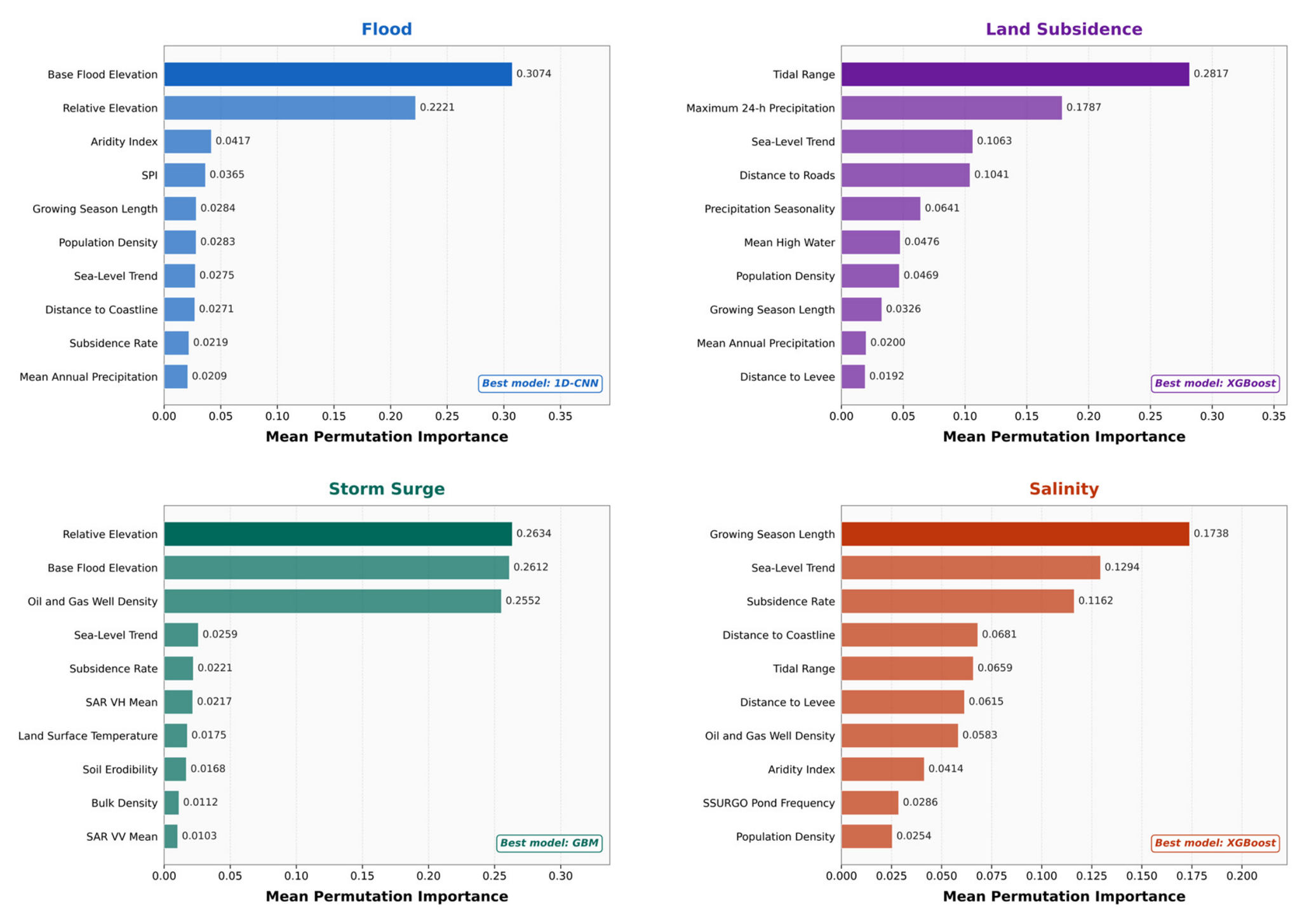
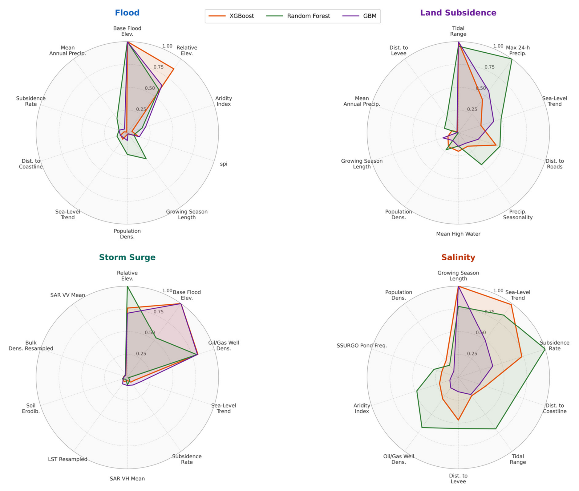
Permutation-based feature importance identified hazard-specific factor rankings with partially shared predictors across hazards, each consistent with the geomorphic and anthropogenic context of coastal Louisiana (

Table 6. Top 10 conditioning factors per hazard ranked by aggregate permutation importance (mean across XGBoost, RF, GBM) for Terrebonne Parish.

Rank	Flood	Imp.	Subsidence	Imp.	Storm Surge	Imp.	Salinity	Imp.
1	Base Flood Elev.	0.307	Tidal Range	0.282	Relative Elev.	0.263	Grow. Season Len.	0.174
2	Relative Elev.	0.222	Max 24hr Precip.	0.179	Base Flood Elev.	0.261	Sea-Level Trend	0.129
3	Aridity Index	0.042	Sea-Level Trend	0.106	Oil Gas Well Dens.	0.255	Subsidence Rate	0.116
4	SPI	0.036	Dist. to Roads	0.104	Sea-Level Trend	0.026	Dist. to Coastline	0.068
5	Grow. Season Len.	0.028	Precip. Seasonality	0.064	Subsidence Rate	0.022	Tidal Range	0.066
6	Population Density	0.028	Mean High Water	0.048	SAR VH	0.022	Dist. to Levee	0.061
7	Sea-Level Trend	0.028	Population Density	0.047	LST	0.018	Oil Gas Well Dens.	0.058
8	Dist. to Coastline	0.027	Grow. Season Len.	0.033	Soil Erodibility	0.017	Aridity Index	0.041
9	Subsidence Rate	0.022	Mean Ann. Precip.	0.020	Bulk Density	0.011	Pond Frequency	0.029
10	Mean Ann. Precip.	0.021	Dist. to Levee	0.019	SAR VV	0.010	Population Density	0.025

; Figure 7 and Figure 8). For flood susceptibility, Base Flood Elevation (mean importance = 0.307) and relative elevation (0.222) dominate, with every remaining factor an order of magnitude lower: BFE directly encodes FEMA’s engineering assessment of flood exposure, while relative elevation captures the subtle but decisive micro-topographic relief of an otherwise nearly flat deltaic surface. For land subsidence, Tidal Range (0.282) leads, capturing the tidal loading cycle that drives cyclical consolidation of estuarine sediments, followed by maximum 24 h precipitation (0.179), Sea-Level Trend (0.106), and distance to roads (0.104), the latter tracing the developed natural-levee corridors that separate compaction-prone backswamp from more stable ground. For storm surge, three predictors are statistically inseparable at the top: relative elevation (0.263), Base Flood Elevation (0.261), and oil and gas well density (0.255), the last functioning as a compound spatial indicator of exposed coastal zones characterized by extensive canal dredging, land loss, and reduced natural attenuation capacity. For salinity intrusion, growing season length (0.174) leads as a smooth climatic proxy for the parish’s north–south freshwater–marine gradient, followed by Sea-Level Trend (0.129), the primary marine forcing of saltwater encroachment along the bayou and canal network, and subsidence rate (0.116). The radar charts (Figure 8) show that the three tree ensembles agree closely on the identity of each hazard’s leading predictors, with GBM assigning the largest absolute F1-decreases to the top factors in all four hazards. Sea-Level Trend is the only factor ranking in the top 10 for all four hazards, establishing relative sea-level acceleration as the cross-cutting vulnerability indicator of Terrebonne Parish’s compound coastal hazard environment; oil and gas well density is top-tier for storm surge and top-10 for salinity, marking the industrial landscape signature as the leading anthropogenic gradient.

5.6. Susceptibility Maps and Multi-Hazard Composite Index

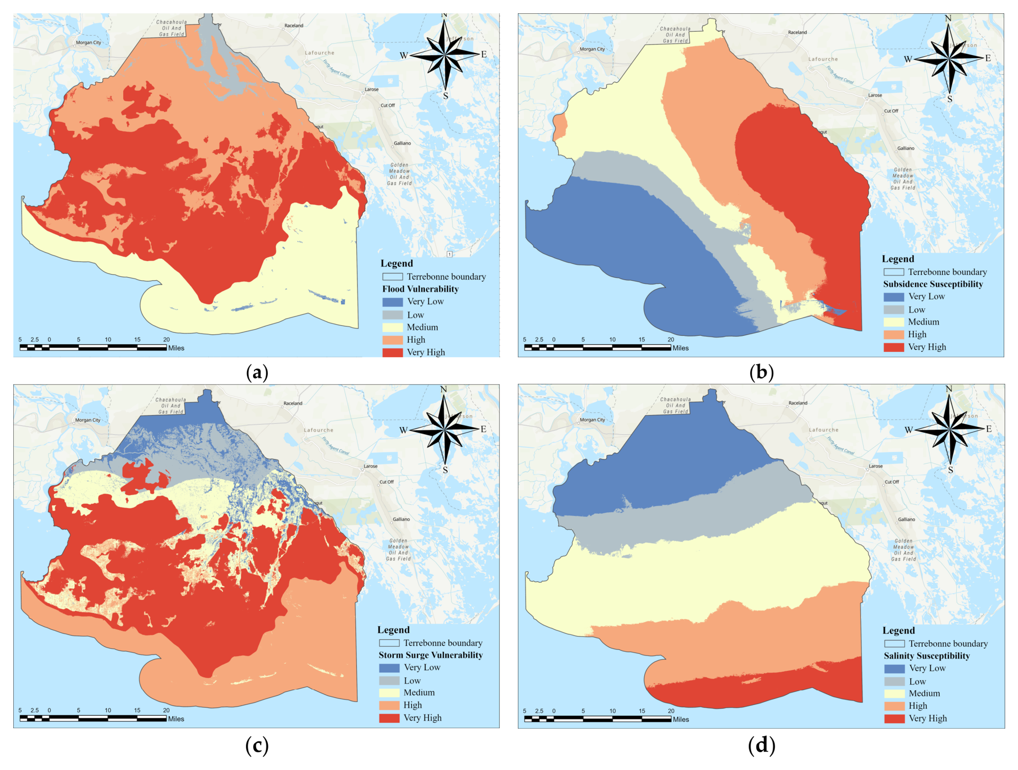
Five-class susceptibility maps at 30 m resolution were generated for each hazard across all 9,266,642 pixels within the Terrebonne Parish administrative boundary (Figure 9). This pixel count corresponds to approximately 8340 km², which exceeds the parish’s ~5500 km² land-and-transitional-water extent because the administrative boundary polygon encompasses open-water tidal bodies and nearshore Gulf of Mexico areas south of the barrier islands. Pixels classified as open water by NLCD 2021 were retained in susceptibility map output but excluded from training sample selection. Flood susceptibility (Figure 9a) is strongly skewed toward elevated susceptibility: Very Low (12,728 pixels; 0.1%), Low (185,426; 2.0%), Moderate (1,554,686; 16.8%), High (5,005,678; 54.0%), and Very High (2,508,124; 27.1%), with over 81% of the parish classified as High or Very High. This pattern reflects the near-universal low relief and marginal elevation above sea level characteristic of the Mississippi deltaic plain. Land subsidence (Figure 9b) exhibits a more spatially differentiated, Moderate-dominated distribution: Very Low (17.2%), Low (6.4%), Moderate (48.3%), High (14.2%), and Very High (13.9%), with highest susceptibility concentrated in zones of active hydrocarbon extraction and unconsolidated Holocene sediments. Storm surge (Figure 9c) mirrors a flood’s distribution toward high susceptibility (~80% High or Very High), reflecting the extensive low-lying coastal exposure of the southern parish. Salinity intrusion (Figure 9d) exhibits a pronounced north–south gradient under the upgraded 21-station kriged labels: Very Low (1.4%), Low (16.1%), Moderate (22.8%), High (18.2%), and Very High (41.5%), with the Very High class dominated by the open-Gulf and lower-estuarine waters south of the barrier islands (euhaline by construction) and the freshest classes confined to the northern upland margins. The map should accordingly be read jointly with the land-masked treatment of open water described in Section 4 and the kriging-variance surface (Supplementary Figure S2), which flags the under-sampled interior marsh as the zone of greatest label uncertainty.

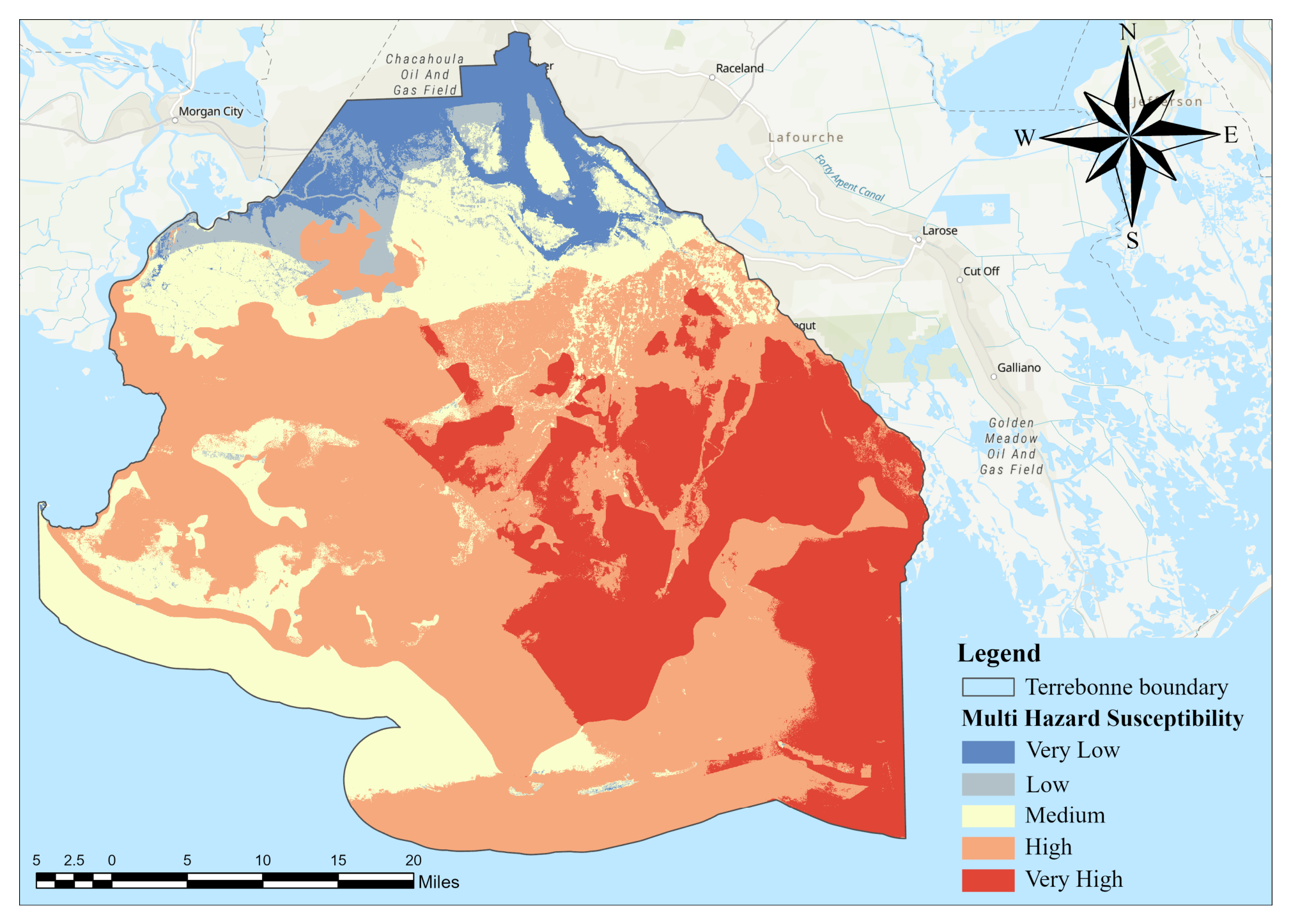
The composite MHSI (Figure 10) integrates all four normalized hazard susceptibility surfaces into a continuous compound risk index (mean = 0.675, std = 0.122, range = 0.188–0.938). Southern Terrebonne records the highest composite MHSI values (>0.75), where all four hazards simultaneously converge at elevated susceptibility identifying this zone as the highest-priority area for integrated coastal risk reduction and climate adaptation investment. The north–south MHSI gradient reflects the region’s geomorphic transition from relatively stable Pleistocene upland terraces in the north to actively subsiding, tidally influenced Holocene depositional plains and open water in the south. Communities situated within this high-MHSI southern zone face compounding hazard interactions: storm surge-induced flooding accelerates organic soil oxidation and subsidence while simultaneously driving saltwater intrusion that degrades freshwater resources and further compromises marsh structural integrity.

5.7. SAEML Ensemble Meta-Learner Results

Table 7. SAEML performance versus the strongest single base model per hazard (Terrebonne Parish). Base model selected by interleaved-block CV F1-macro; CV values are mean ± SD across five folds; ΔCV = SAEML CV F1 minus base CV F1 in percentage points; Train = total SAEML training time (all three stages).

Hazard	Best Base Model (CV)	Base Holdout F1	Base CV F1 (Mean ± SD)	SAEML Holdout F1	SAEML CV F1 (Mean ± SD)	ΔCV (pp)	SAEML Train (h)
Flood	1D-CNN	0.923	0.947 ± 0.013	0.950	0.936 ± 0.031	−1.10	1.46
Subsidence	XGBoost	0.919	0.949 ± 0.014	0.929	0.944 ± 0.016	−0.54	1.89
Storm Surge	GBM	0.865	0.886 ± 0.025	0.867	0.880 ± 0.028	−0.66	1.60
Salinity	XGBoost	0.644	0.669 ± 0.039	0.625	0.652 ± 0.020	−1.75	1.25

presents SAEML performance alongside the strongest single model per hazard. Under interleaved-block spatial cross-validation, the criterion on which operational model selection must rest, the meta-learner achieved F1-macro of 0.936 ± 0.031 for flood, 0.944 ± 0.016 for subsidence, 0.880 ± 0.028 for storm surge, and 0.652 ± 0.020 for salinity, trailing the best single base model in every case (0.947, 0.949, 0.886, and 0.669, respectively; deficits of 0.5–1.8 percentage points). On the spatially blocked holdout zone, the differences are mixed and inconsistent in sign: modest gains for flood (0.950 versus 0.923), subsidence (0.929 versus 0.919), and storm surge (0.867 versus 0.865), and a loss for salinity (0.625 versus 0.644), all within fold-level variability. These results were obtained at a total SAEML training cost of 22,293 s (≈6.2 h), roughly five times the 71 min required to train all 32 final base models. Calibrated probability stacking with agreement meta-features therefore does not improve upon cross-validation-guided single-model selection for any of the four hazards.

6. Discussion

6.1. Algorithm Performance: ML Versus DL

Model superiority proved hazard-dependent rather than algorithmic. The 1D-CNN, XGBoost, and GBM each led different hazards under holdout evaluation, while LSTM was consistently the weakest performer regardless of hazard. The 1D-CNN’s advantage for flood susceptibility is consistent with findings by Ullah et al. [8], who demonstrated that convolutional filters effectively capture local multi-factor interaction patterns; the co-occurrence of low Base Flood Elevation, low relative elevation, and proximity to drainage represents an interaction structure that additive tree models encode less efficiently through axis-aligned splits. XGBoost’s superiority for land subsidence reflects the dominance of categorical and semi-ordinal predictors (soil drainage class, hydrologic soil group) that gradient boosting partitions efficiently through asymmetric splits on ordered feature thresholds [13]. GBM’s advantage for storm surge, the hazard most strongly governed by gradual coastal-proximity and elevation gradients, may reflect its sequential residual correction, which iteratively captures diffuse, nonlinear boundary behavior more effectively than deep networks trained on relatively small samples [20]. Salinity proved the most difficult hazard for every algorithm (best holdout F1-macro of 0.644, XGBoost): salinity dynamics integrate multiple weakly observed drivers, and the labels inherit the irreducible uncertainty of kriging from a sparse station network (quantified by the published variance surface, Supplementary Figure S2), so the performance ceiling reflects the evidence base rather than any algorithmic deficiency. LSTM’s consistent underperformance provides an important architectural caution: sequential memory networks designed for ordered time series impose an artificial ordering on static tabular inputs, introducing optimization overhead without capturing genuine spatial structure, contradicting the assumption underlying several recent DL applications in geospatial susceptibility mapping [7].

The strict contiguous-zone results (Section 5.4) push this interpretation from algorithms to processes: the four hazards are divided into two transfer regimes. Flood and storm surge, whose dominant predictors encode portable physical relationships among terrain, coastal proximity, and inundation, retained most of their skill under strict evaluation (best F1-macro of 0.826 and 0.751, respectively). Subsidence and salinity, learned from regionally specific interpolated fields, the east–west subsidence-rate gradient and the smooth kriged salinity surface, degraded sharply (0.411 and 0.438): models trained on such labels partly memorize regional position through spatially structured predictors and cannot reproduce it in unseen zones. Transferability is thus governed less by algorithm family than by whether a hazard’s predictive structure is physically portable, a geomorphological property of the hazard itself, not of the learner.

6.2. Validation Design and Spatial Transferability

The three-design comparison in Section 5.4 has direct implications for how susceptibility benchmarks should be produced and read. The near-equivalence of blocked holdout and interleaved-block CV shows that the mere use of spatial blocks, the most common implementation of “spatial cross-validation” in the susceptibility literature, does not deliver the honest assessment it is widely assumed to provide: without buffering and contiguity, fold geometry leaves every test sample embedded in training context, and the evaluation measures interpolation rather than transfer. The strict contiguous-zone results quantify the difference: hazard-mean F1-macro declines of 15 (flood), 17 (storm surge), 26 (salinity), and 56 (subsidence) percentage points relative to interleaved-block CV (grand mean 29 points), accompanied by a re-ranking in which the sequence architectures (LSTM, CNN-LSTM) fall to the bottom for every hazard and the interleaved winner survives only for flood and salinity. The magnitude of decline is itself diagnostic: hazards whose predictive structure is physically portable lose 15–17 points, whereas hazards learned from regionally specific spatial fields lose 26–56 points. Practical mitigation follows directly: model selection for deployment at unsampled locations should rest on strict spatial evaluation; the maps are most defensible for relative ranking and regional prioritization; zone-level performance variability identifies where new ground truth would most improve transferability; and spatial-context architectures, domain adaptation, and uncertainty quantification are the methodological remedies pursued in Future Work. Following Wadoux et al. [18], the strict design may itself be conservative for prediction within densely sampled areas, true performance for infill mapping lies between the interleaved and strict estimates, and the pair should be reported together as bracketing bounds.

6.3. Hazard-Specific Factor Insights

A caveat frames this section: permutation importance measures predictive contribution under the trained model, not causal influence. A highly ranked predictor may act as a statistical proxy for an unmeasured driver, and importance among correlated predictors (Section 4.2) can be shared or diluted across the correlated group. The interpretations that follow therefore treat the rankings as hypotheses whose physical plausibility is assessed against independent process knowledge. The clearest example is oil and gas well density: its high ranking for subsidence is consistent with documented extraction-induced compaction in coastal Louisiana, but the variable plausibly also proxies the broader spatial footprint of hydrocarbon activity, dredged access canals, spoil banks, and associated wetland degradation, so its importance should be read as marking the industrial landscape signature rather than isolating fluid withdrawal as a mechanism. Its comparably high rank for storm surge susceptibility invites the same two-level reading. Mechanistically, hydrocarbon infrastructure is a genuine modifier of surge dynamics in Terrebonne: the dredged access-canal network provides low-friction conduits that accelerate and extend surge propagation into the interior marsh; canal spoil banks disrupt natural sheet-flow drainage; and extraction-enhanced subsidence and wetland fragmentation progressively remove the vegetated surface roughness that attenuates surge. Statistically, however, well density is also strongly spatially confounded with coastal position; wells concentrate in the low-lying southern marshes where surge susceptibility is highest for reasons of elevation and proximity alone, so its importance score bundles genuine anthropogenic amplification with simple coastal geography. Distinguishing these contributions rigorously would require process-based surge modeling with and without canal networks (e.g., ADCIRC scenario runs), which we identify in Future Work as the appropriate test of the amplification hypothesis; within a statistical framework, the ranking establishes that the industrial footprint carries substantial predictive information about surge susceptibility, consistent with, but not proof of, the documented physical pathways.

The permutation importance rankings align with and extend prior geomorphic and risk literature on Louisiana coastal dynamics. For flood susceptibility, the two dominant predictors are Base Flood Elevation (0.307) and relative elevation (0.222), with all remaining factors an order of magnitude lower, a terrain–hydraulic dominance consistent with inundation control by elevation relative to local drainage in near-flat deltaic terrain. Both predictors reward process-level scrutiny. BFE values are themselves outputs of FEMA’s process-based hydraulic and coastal modeling, so the predictor imports distilled engineering hydraulics, modeled water-surface elevations for the 1-annual-chance event, into the statistical framework, and its top rank partly reflects genuine process content. Two caveats bound this reading: BFE shares provenance with the FEMA flood zones from which the flood labels derive, so although the zone classification itself is excluded from the flood predictor set (Table 2), BFE retains a partial, indirect association with the label source and should be interpreted with corresponding caution; and, as established above, importance rankings identify association rather than mechanism. Soil erodibility, prominent in the impurity-based screening of the originally submitted analysis, falls to rank 12 under permutation importance, impurity-based measures are known to inflate continuous, high-cardinality predictors and to share credit among correlated soil attributes, although its residual contribution retains a coherent interpretation as a proxy for the fine-textured, poorly drained soils of flood-prone depositional environments. Tidal Range as the top subsidence predictor (0.282) accords with Jankowski et al.’s [16] finding that tidal forcing is a primary short-term control on vertical displacement in Louisiana’s coastal plain, with repetitive tidal loading consolidating estuarine sediments; its co-occurrence with precipitation-regime factors (maximum 24 h precipitation, 0.179) and Sea-Level Trend (0.106) indicates that the models read subsidence susceptibility chiefly from the coastal-gradient and hydroclimatic setting of compaction-prone deposits. For storm surge, three predictors are statistically inseparable at the top: relative elevation (0.263), Base Flood Elevation (0.261), and oil and gas well density (0.255). The prominence of well density alongside the two terrain–hydraulic factors corroborates Turner and McClenachan [4], who attributed over 35,000 wetland cuts to oil and gas infrastructure, reducing natural surge attenuation and creating direct inundation pathways into previously sheltered interior zones; the mechanistic and confounding aspects of this predictor are examined below. For salinity, growing season length (0.174) leads, followed by Sea-Level Trend (0.129) and subsidence rate (0.116): the models read salinity susceptibility from the parish’s north–south freshwater–marine gradient, growing season length acting as a smooth climatic proxy for that gradient, combined with marine forcing and coupled land-surface lowering, consistent with the regionally structured character of the kriged salinity labels (Section 5.4). Across hazards, Sea-Level Trend is the only factor ranking in the top 10 for all four, identifying relative sea-level acceleration as the parish’s master compound-risk gradient, while oil and gas well density is top-tier for storm surge and top-10 for salinity, together arguing directly for integrated multi-hazard governance rather than single-hazard management. The definitive test of these process interpretations, coupling the statistical framework to process-based hydrologic and hydraulic simulation (rainfall–runoff modeling over the soil grid; HEC-RAS or ADCIRC water-surface fields in place of their statistical proxies), is identified in Future Work.

Positioned against the broader multi-hazard literature, these results agree on some dimensions and diverge instructively on others. The holdout performance reported here (best F1-macro of 0.644–0.923) is consistent with the high skill reported for CNN-based multi-hazard mapping in Pakistan [8] and hybrid statistical–Machine Learning mapping in Turkey [6]; however, those studies evaluated under random or single-holdout designs, so their accuracies are directly comparable only to this study’s optimistic bounds. Under buffered contiguous-zone evaluation, scores here fall by 12–54 percentage points, a caveat that plausibly extends to published multi-hazard accuracies in general. Predictor-importance patterns likewise agree at the top of the rankings: terrain elevation and hydrologic or coastal proximity dominate here as in terrestrial multi-hazard studies [6,7,8]. By contrast, the prominence of anthropogenic-infrastructure factors, oil and gas well density, and canal density, is distinctive to the deltaic setting and has no counterpart in the terrestrial literature. Methodologically, the retain-and-disclose treatment of correlated predictors adopted here contrasts with the factor-selection strategies of statistical susceptibility frameworks such as the GIS Matrix Method [40], which prune predictors before modeling; both are defensible, but pruning optimizes single-factor interpretability whereas retention preserves complementary information for prediction across four physically distinct hazards. Finally, the emphasis this study places on label quality, a published kriging variance surface, and leave-one-station-out validation, parallels growing attention to inventory completeness and automated quality control in susceptibility research [41]: in both cases, the reliability ceiling of the final map is set by the evidence base rather than by the learning algorithm. The susceptibility patterns themselves, compound risk concentrated along the low-lying coastal fringe, mirror the coastal-gradient organization reported wherever surge, flooding, and salinization co-occur in deltaic settings.

6.4. SAEML: Ensemble Meta-Learning for Spatial Generalization

The ensemble results warrant a candid operational reading. SAEML matches but does not exceed the best single models: its cross-validated F1-macro trails the best base model by 0.5–1.8 percentage points on every hazard, and its holdout differences (−1.9 to +2.7 points) are inconsistent in sign and within fold-level variability. The mechanistic explanation is error correlation: all eight base models learn from the same predictor stack and the same labels, so their errors are strongly correlated and the agreement-based meta-features carry little complementary information, where the base models fail, they tend to fail together. Set against a training cost roughly five times that of all base models combined (≈6.2 h versus 71 min), the operational recommendation is unambiguous: for multi-hazard susceptibility mapping, benchmark a diverse model set under spatially honest cross-validation and deploy the best single model; the resources that stacking consumes are better invested in strict spatial evaluation, improved labels, and uncertainty quantification. The meta-learner’s model-disagreement output retains diagnostic value as a spatial uncertainty indicator, and we retain it for that purpose rather than for prediction. We note that this negative finding was established under the interleaved-block design; there is no reason to expect stacking of the same base models to fare better under the strict contiguous-zone design, where all base models lose skill.

6.5. Implications for Coastal Risk Management

The susceptibility maps and composite MHSI (Figure 10) provide spatially explicit, quantitatively grounded information with direct relevance to coastal risk management in Terrebonne Parish. The composite index consistently identifies southern Terrebonne, the zone of highest MHSI values (>0.75), as the highest-priority area for integrated risk reduction investment, where concurrent exposure to all four hazards creates compound vulnerability that no single-hazard management strategy can adequately address. The finding that over 81% of the parish falls in the High or Very High flood susceptibility class, and nearly 80% for storm surge, indicates the need to shift risk communication from event-driven response to systematic long-term resilience planning. Practical applications include prioritization of elevated building standards and managed retreat zones in the High and Very High susceptibility classes; routing of infrastructure investment (levees, floodgates, living shorelines) toward the high-MHSI southern zone; integration of salinity and subsidence susceptibility surfaces into freshwater supply planning and structural engineering design standards; and targeted land-use regulation restricting high-density development in areas where two or more hazards intersect at elevated susceptibility levels. One important caveat is that the strict contiguous-zone results demonstrate substantial performance degradation at truly new locations (best-model F1-macro of 0.41–0.83, hazard-dependent), implying that pixel-level predictions in poorly sampled subregions should be treated as indicative rather than authoritative and supplemented with targeted field validation campaigns before informing high-stakes regulatory decisions. The susceptibility maps are most reliable and defensible for regional-scale pattern identification, relative risk ranking among sub-units of the parish, and prioritization of field investigation resources.

Translating the continuous index into operational tiers requires thresholds tied to interventions, and the discrete structure of the land-masked MHSI provides natural break points. Because the index is the mean of four ordinal class values, it moves in steps of 1/16, and its land distribution is strongly structured: 56.6% of land pixels average exactly High susceptibility (MHSI = 0.75) across the four hazards, a plateau reflecting the parish’s pervasive baseline exposure. Only 4.0% of land exceeds this plateau (MHSI ≥ 0.8125), marking locations where Very High classes accumulate across multiple hazards. Three decision tiers follow. Tier 1, critical priority (MHSI ≥ 0.8125; 4.0% of land): the defensible target for the most consequential interventions, voluntary acquisition and relocation eligibility, exclusion of new critical facilities, and first-ranked structural protection investment. Tier 2, elevated management (MHSI = 0.75; 56.6% of land): enhanced building standards (freeboard above Base Flood Elevation), stormwater and drainage upgrading, and hazard-disclosure requirements; because the composite cannot discriminate within this plateau, prioritization inside Tier 2 should rest on the per-hazard composition (number of Very High classes) and on asset exposure from the parcel overlay described below. Tier 3, standard management (MHSI < 0.75; 39.4% of land): baseline code compliance and periodic reassessment. These tiers are screening thresholds, not regulatory determinations: Tier 1 assignment warrants site-level verification, and the tier boundaries themselves should be revisited as the index is updated, since they are properties of the current hazard-class distributions rather than fixed physical constants. Realistic integration proceeds through institutional mechanisms that already exist. First, the Terrebonne Parish Hazard Mitigation Plan, updated on FEMA’s five-year cycle, requires a spatially explicit hazard identification and risk assessment; the four susceptibility maps and the land-masked MHSI can serve directly as that assessment’s evidence layer, replacing the parish-uniform hazard rankings typical of such plans with 30 m spatial differentiation. Second, Louisiana’s Coastal Master Plan screens candidate protection and restoration projects through predictive modeling at the coast-wide scale; the susceptibility surfaces provide a parish-scale complement for ranking nonstructural projects, home elevation, acquisition, and floodproofing, within Terrebonne. Third, FEMA’s Community Rating System awards flood-insurance premium reductions for open-space preservation and enhanced regulatory standards targeted to mapped hazard areas; the High and Very High flood and surge classes constitute a defensible targeting layer for such credits. A concrete decision-support workflow illustrates the intended use: overlay the land-masked MHSI top decile with parcel boundaries and critical-infrastructure locations (schools, water intakes, emergency facilities, evacuation routes); rank exposed assets by composite susceptibility; and use that ranking to sequence mitigation investments in annual capital planning. Two caveats bound this use. Susceptibility classifications should trigger site-level verification rather than serve as parcel-level regulatory determinations, because strict spatial evaluation (Section 5.4) shows that accuracy degrades away from well-characterized areas; and because of the balanced sampling design (Section 4.4), decisions should rest on class assignments and relative rankings rather than on raw predicted probabilities.

Because no single observable corresponds to “multi-hazard susceptibility,” evaluation of the composite index proceeds to three levels. First, its components are validated individually: each hazard layer carries holdout and cross-validated performance under three spatial designs, and the salinity layer additionally carries a published interpolation-variance surface. Second, the index’s construction is tested for robustness: the weighting sensitivity analysis shows the land-masked top-decile priority zone is 88–94% stable under twofold up-weighting of any single hazard, while the all-pixel index is substantially more weight-sensitive because open-water pixels dominate its upper tail, itself a reason to prefer the land-masked index for prioritization. Third, independent event-based evaluation is the appropriate next step: the high-priority zone can be tested for concordance with historical multi-hazard footprints, Hurricane Ida’s damage assessments and National Flood Insurance Program claim distributions, surveyed high-water marks, post-storm wetland-loss mapping, and with the hazard zones already used in parish mitigation planning. Such retrospective concordance analysis quantifies decision-relevant skill (whether the index ranks damaged locations above undamaged ones) without requiring the composite to predict any single event and is identified as a priority for future work.

7. Limitations

Several limitations constrain these findings; each is paired with a research direction in Section 9.

Label uncertainty: Hazard labels derive from documented decision rules applied to existing datasets rather than field observation. This is most consequential for salinity, where labels rest on ordinary kriging of 21 stations (leave-one-station-out RMSE = 3.40 PSU; R² = 0.82); the published kriging-variance surface maps this uncertainty, which is greatest in the under-sampled interior marsh, and salinity’s lower classification ceiling across all models is consistent with it.

Validation design: Even the strict contiguous-zone design cannot remove regional-scale gradients (variogram effective ranges of 22–150 km) within a single parish; transfer estimates to genuinely distant settings require multi-parish evaluation. Conversely, following Wadoux et al. [18], strict spatial CV may understate accuracy for infill prediction within the sampled domain; the interleaved and strict designs are therefore reported as bracketing bounds.

Static scope: The framework maps static susceptibility, omitting seasonal variability, long-term subsidence and sea-level trajectories, and future climate and land-use scenarios; trend variables in the predictor stack embed recent dynamics, but the maps are a contemporary snapshot.

Scale and data representation: The 30 m grid under-represents wetland transition zones narrower than the grid spacing; several predictors have coarse native resolutions; and six DEM-derived variables are uninformative on this near-flat terrain, reducing the effective predictor count to 59.

Modeling design: Pixels are classified independently of their neighbors, and class-balanced sampling means predicted probabilities are not prevalence-calibrated (Section 4.4).

Ensemble finding and geographic scope: The Spatially Aware Ensemble Meta-Learner did not outperform cross-validation-guided single-model selection on any hazard (cross-validated F1 deficits of 0.5–1.8 percentage points at roughly five times the training cost), and this negative finding was established under interleaved-block evaluation rather than the strict contiguous-zone design. All results pertain to Terrebonne Parish; transferability to neighboring parishes requires explicit validation.

8. Conclusions

This study sets out to determine whether four co-occurring coastal hazards can be credibly mapped within a single Machine Learning framework, and what honest spatial evaluation of such a framework requires. Four contributions emerge.

First, a reproducible template for unified multi-hazard susceptibility assessment: a common 30 m predictor stack across ten thematic categories, documented evidence-based labeling with per-hazard circularity control, and an identical benchmarking protocol across eight ML and DL algorithms, to the best of our knowledge the first such controlled design spanning flooding, subsidence, storm surge, and salinity intrusion.

Second, a quantitative demonstration that validation design governs apparent transferability. Spatially blocked holdout and interleaved-block cross-validation, the field’s most common “spatially aware” evaluations, proved statistically indistinguishable, while buffered contiguous-zone evaluation revealed genuine transfer degradation of 12 (flood) to 54 (subsidence) percentage points in best-model F1-macro. The practical prescription is concrete: spatial blocking without contiguity and buffering does not deliver honest evaluation, and published block-CV susceptibility accuracies should be read as upper bounds on transferability.

Third, an empirically grounded operational recommendation on ensembles: spatially aware calibrated stacking of all eight base models failed to improve on cross-validation-guided single-model selection for any hazard and cross-validated F1-macro deficits of 0.5–1.8 percentage points at roughly five times the training cost, so operational multi-hazard mapping is better served by benchmarking a diverse model set under spatially honest evaluation and deploying the best single model.

Fourth, management-ready outputs with quantified confidence: five-class maps for all four hazards; a salinity surface with published interpolation uncertainty; and a composite index reported parish-wide and land-masked, whose southern-Terrebonne priority zone is robust to twofold reweighting of any single hazard. Because the parish’s coupled hazard system typifies subsiding deltas worldwide, both the framework and these evaluation-design findings extend beyond coastal Louisiana.

9. Future Work

Future research directions follow directly from the limitations in Section 7. Addressing label uncertainty, the priority is strengthening the evidence base: event-based labels, post-storm damage assessments, surveyed high-water marks, observed salinity exceedances, and targeted densification of the salinity monitoring network, guided by the published kriging-variance surface toward the under-sampled interior marsh, would raise the salinity performance ceiling and enable the event-based concordance testing of the composite index outlined in Section 6.5. Integration of satellite-derived salinity proxies and hydrodynamic model output (e.g., Delft3D or ADCIRC-based salinity fields) as additional evidence layers is the natural next upgrade of the salinity evidence base. Addressing the validation-design constraint of single-parish evaluation, the framework should be applied to Lafourche and Plaquemines Parishes with cross-parish training and testing, complementing the within-parish strict spatial CV reported here; spatial-context architectures (graph neural networks, patch-based models) and domain adaptation are the natural modeling remedies for the transfer degradation the strict design quantifies. Addressing static scope, incorporating time-series predictors and scenario forcing, relative sea-level trajectories, land-use change, and marsh-loss projections would convert the contemporary snapshot into dynamic susceptibility trajectories. Addressing scale, the 10 m Sentinel-2 bands and commercial sub-meter imagery could support a multi-scale analysis in which fine-resolution spectral gradients are summarized within each 30 m cell (sub-pixel wetland fraction, edge density), sharpening representation of the narrow marsh transition zones where hazard interactions concentrate. Addressing modeling design, prevalence re-weighting would make predicted probabilities decision-grade rather than rank-grade; conformal prediction or Bayesian methods would attach formal uncertainty statements to each pixel for operational risk communication; and SHAP-based attribution would sharpen mechanistic interpretation of correlated predictor groups (Section 4.2). Finally, addressing the framework’s treatment of the four hazards as parallel mapping targets, explicitly modeling hazard interactions and cascades, surge-triggered flooding and salinization feeding subsidence acceleration, as described in Section 1 and Section 3, are the most scientifically consequential extension: moving from mapping co-located susceptibility to modeling the coupled system that generates it.

References

1. Adewale, A.A. Assessing Coastal Resilience to Sea-Level Rise, Flooding and Extreme Weather Events Using Spatial Data and Big Data Analysis on the United Coast Gulf Coasts. Int. J. Sci. Adv. Technol. (IJSAT) 2025, 16, 2180. [Google Scholar] [CrossRef] [Scilit]
2. Salcedo-Sanz, S.; Ghamisi, P.; Piles, M.; Werner, M.; Cuadra, L.; Moreno-Martínez, A.; Izquierdo-Verdiguier, E.; Muñoz-Marí, J.; Mosavi, A.; Camps-Valls, G. Machine learning information fusion in Earth observation: A comprehensive review. Inf. Fusion 2020, 63, 256–272. [Google Scholar] [CrossRef] [Scilit]
3. Couvillion, B.R.; Beck, H.; Schoolmaster, D.; Fischer, M. Land Area Change in Coastal Louisiana (1932 to 2016); USGS Scientific Investigations Map 3381; USGS Publications Warehouse: Reston, VA, USA, 2017.
4. Turner, R.E.; McClenachan, G. Reversing wetland death from 35,000 cuts. PLoS ONE 2018, 13, e0207717. [Google Scholar] [CrossRef] [Scilit] [PubMed]
5. NOAA NCEI. Billion-Dollar Weather and Climate Disasters; National Centers for Environmental Information: Asheville, NC, USA, 2023. Available online: https://www.ncei.noaa.gov/access/billions/ (accessed on 1 January 2026).
6. Karakas, G.; Kocaman, S.; Gokceoglu, C. A hybrid multi-hazard susceptibility assessment model for a basin in Elazig Province, Turkiye. Int. J. Disaster Risk Sci. 2023, 14, 326–341. [Google Scholar] [CrossRef] [Scilit]
7. Sreevalsan-Nair, J.; Mundayatt, A. Evolution of data-driven single- and multi-hazard susceptibility mapping and emergence of deep learning methods. arXiv 2025, arXiv:2502.09045. [Google Scholar]
8. Ullah, K.; Wang, Y.; Fang, Z.; Wang, L.; Rahman, M. Multi-hazard susceptibility mapping based on Convolutional Neural Networks. Geosci. Front. 2022, 13, 101425. [Google Scholar] [CrossRef] [Scilit]
9. Achu, A.L.; Aju, C.D.; Di Napoli, M.; Prakash, P.; Gopinath, G.; Shaji, E.; Chandra, V. Machine-learning based landslide susceptibility modelling with emphasis on uncertainty analysis. Geosci. Front. 2023, 14, 101657. [Google Scholar] [CrossRef] [Scilit]
10. Park, S.; Kim, J. The predictive capability of a novel ensemble tree-based algorithm for assessing groundwater potential. Sustainability 2021, 13, 2459. [Google Scholar] [CrossRef] [Scilit]
11. Waleed, M.; Sajjad, M. High-resolution flood susceptibility mapping and exposure assessment in Pakistan: An integrated artificial intelligence, machine learning and geospatial framework. Int. J. Disaster Risk Reduct. 2025, 121, 105442. [Google Scholar] [CrossRef] [Scilit]
12. Tepetidis, N.; Benekos, I.; Iliopoulou, T.; Dimitriadis, P.; Koutsoyiannis, D. Combining machine learning models and satellite data of an extreme flood event for flood susceptibility mapping. Water 2025, 17, 2678. [Google Scholar] [CrossRef] [Scilit]
13. Chen, T.; Guestrin, C. XGBoost: A scalable tree boosting system. In Proceedings of the 22nd ACM SIGKDD International Conference on Knowledge Discovery and Data Mining, San Francisco, CA, USA, 13–17 August 2016; pp. 785–794. [Google Scholar]
14. Riche, A.; Drias, A.; Guermoui, M.; Gherib, T.; Boulmaiz, T.; Souissi, B.; Melgani, F. A novel hybrid deep-learning approach for flood-susceptibility mapping. Remote Sens. 2024, 16, 3673. [Google Scholar] [CrossRef] [Scilit]
15. Chen, R.; Wang, X.; Zhang, W.; Zhu, X.; Li, A.; Yang, C. A hybrid CNN-LSTM model for typhoon formation forecasting. Geoinformatica 2019, 23, 375–396. [Google Scholar] [CrossRef] [Scilit]
16. Jankowski, K.L.; Tornqvist, T.E.; Fernandes, A.M. Vulnerability of Louisiana’s coastal wetlands to present-day rates of relative sea-level rise. Nat. Commun. 2017, 8, 14792. [Google Scholar] [CrossRef] [Scilit] [PubMed]
17. Roberts, D.R.; Bahn, V.; Ciuti, S.; Boyce, M.S.; Elith, J.; Guillera-Arroita, G.; Hauenstein, S.; Lahoz-Monfort, J.J.; Schröder, B.; Thuiller, W.; et al. Cross-validation strategies for data with temporal, spatial, hierarchical, or phylogenetic structure. Ecography 2017, 40, 913–929. [Google Scholar] [CrossRef] [Scilit]
18. Wadoux, A.M.J.-C.; Heuvelink, G.B.M.; de Bruin, S.; Brus, D.J. Spatial cross-validation is not the right way to evaluate map accuracy. Ecol. Model. 2021, 457, 109692. [Google Scholar] [CrossRef] [Scilit]
19. Breiman, L. Random forests. Mach. Learn. 2001, 45, 5–32. [Google Scholar] [CrossRef] [Scilit]
20. Friedman, J.H. Greedy function approximation: A gradient boosting machine. Ann. Stat. 2001, 29, 1189–1232. [Google Scholar] [CrossRef] [Scilit]
21. Vapnik, V.N. The Nature of Statistical Learning Theory; Springer: New York, NY, USA, 1995. [Google Scholar]
22. Hochreiter, S.; Schmidhuber, J. Long short-term memory. Neural Comput. 1997, 9, 1735–1780. [Google Scholar] [CrossRef] [Scilit] [PubMed]
23. Wolpert, D.H. Stacked generalization. Neural Netw. 1992, 5, 241–259. [Google Scholar] [CrossRef] [Scilit]
24. Peel, M.C.; Finlayson, B.L.; McMahon, T.A. Updated world map of the Köppen-Geiger climate classification. Hydrol. Earth Syst. Sci. 2007, 11, 1633–1644. [Google Scholar] [CrossRef] [Scilit]
25. Alshehri, B.; Zhang, Z.; Liu, X. A review of Google Earth Engine for land use and land cover change analysis. ISPRS Int. J. Geo-Inf. 2025, 14, 416. [Google Scholar] [CrossRef] [Scilit]
26. Gorelick, N.; Hancher, M.; Dixon, M.; Ilyushchenko, S.; Thau, D.; Moore, R. Google Earth Engine: Planetary-scale geospatial analysis for everyone. Remote Sens. Environ. 2017, 202, 18–27. [Google Scholar] [CrossRef] [Scilit]
27. PRISM Climate Group. PRISM Climate Data, Oregon State University. 2023. Available online: http://prism.oregonstate.edu (accessed on 1 January 2026).
28. Fick, S.E.; Hijmans, R.J. WorldClim 2: New 1-km spatial resolution climate surfaces for global land areas. Int. J. Climatol. 2017, 37, 4302–4315. [Google Scholar] [CrossRef] [Scilit]
29. NOAA. Center for Operational Oceanographic Products and Services (CO-OPS): Tidal Station Data; National Oceanic and Atmospheric Administration: Washington, DC, USA, 2023. Available online: https://tidesandcurrents.noaa.gov (accessed on 1 January 2026).
30. Jin, S.; Homer, C.; Yang, L.; Danielson, P.; Dewitz, J.; Li, C.; Zhu, Z.; Xian, G.; Howard, D. Overall methodology design for the United States national land cover database 2016 products. Remote Sens. 2019, 11, 2971. [Google Scholar] [CrossRef] [Scilit]
31. Pekel, J.-F.; Cottam, A.; Gorelick, N.; Belward, A.S. High-resolution mapping of global surface water and its long-term changes. Nature 2016, 540, 418–422. [Google Scholar] [CrossRef] [Scilit] [PubMed]
32. FEMA. Flood Insurance Rate Map (FIRM) and Flood Insurance Study: Terrebonne Parish, Louisiana; Federal Emergency Management Agency: Washington, DC, USA, 2023.
33. USDA-NRCS. Soil Survey Geographic (SSURGO) Database; United States Department of Agriculture, Natural Resources Conservation Service: Washington, DC, USA, 2023.
34. Didan, K. MOD13A3 MODIS/Terra Vegetation Indices Monthly L3 Global 1km SIN Grid V006; NASA EOSDIS Land Processes DAAC: Sioux Falls, SD, USA, 2015.
35. Dokka, R.K. Modern-day tectonic subsidence in coastal Louisiana. Geology 2006, 34, 281–284. [Google Scholar] [CrossRef] [Scilit]
36. Kolker, A.S.; Allison, M.A.; Hameed, S. An evaluation of subsidence rates and sea-level variability in the northern Gulf of Mexico. Geophys. Res. Lett. 2011, 38, L21404. [Google Scholar] [CrossRef] [Scilit]
37. Karegar, M.A.; Dixon, T.H.; Malservisi, R. A three-dimensional surface velocity field for the Mississippi Delta: Implications for coastal restoration and flood potential. Geology 2015, 43, 519–522. [Google Scholar] [CrossRef] [Scilit]
38. Hornik, K. Approximation capabilities of multilayer feedforward networks. Neural Netw. 1991, 4, 251–257. [Google Scholar] [CrossRef] [Scilit]
39. Cohen, J. A coefficient of agreement for nominal scales. Educ. Psychol. Meas. 1960, 20, 37–46. [Google Scholar] [CrossRef] [Scilit]
40. Obda, O.; El Kharim, Y.; Obda, I.; Ahniche, M.; Sahrane, R. Landslide Susceptibility Assessment and Factors’ Selection Using the GIS Matrix Method (GMM) in Chefchaouen Province (Northern Morocco). In Recent Research on Geotechnical Engineering, Remote Sensing, Geophysics and Earthquake Seismology (Advances in Science, Technology & Innovation); Springer: Cham, Switzerland, 2024; pp. 197–199. [Google Scholar] [CrossRef] [Scilit]
41. Bounab, A.; El Kharim, Y.; El Kharrim, M.; El Kharrim, A.; Sahrane, R. The performance of landslides frequency-area distribution analyses using a newly developed fully automatic tool. Appl. Geomat. 2024, 16, 789–796. [Google Scholar] [CrossRef] [Scilit]
Figure 1. Geographic location and setting of Terrebonne Parish, coastal Louisiana. The main map shows the parish boundary, major waterways, coastal wetland zones, and infrastructure elements. The inset shows regional context within Louisiana and the Gulf of Mexico.
Ijgi 15 00346 g001
Figure 2. Overview of the methodological workflow illustrating five principal stages: (1) multi-source conditioning factor compilation; (2) hazard label generation and feature exclusion; (3) training and testing of eight ML/DL algorithms; (4) spatial block cross-validation and SAEML development; and (5) susceptibility map generation and composite index derivation.
Ijgi 15 00346 g002
Figure 3. Holdout F1-macro performance of eight ML and DL algorithms across the four coastal hazards (colored bars; * = best model per hazard, evaluated on the spatially blocked fold-four holdout). Dark diamonds show interleaved-block spatial cross-validation F1 (mean ± 1 SD across five folds); red triangles show strict contiguous-zone cross-validation with a 5 km train–test buffer (mean ± 1 SD). The near-coincidence of the diamonds with the bar tops, against the systematically lower triangles, visualizes the central validation-design finding: interleaved-block CV is statistically indistinguishable from holdout evaluation, and only the buffered contiguous-zone design reveals genuine transfer limits, modest for flood and storm surge, severe for land subsidence and salinity intrusion. XGBoost = extreme gradient boosting; SVM = Support Vector Machine; GBM = Gradient Boosting Machine; MLP = Multilayer Perceptron; 1D-CNN = 1-Dimensional Convolutional Neural Network; LSTM = Long Short-Term Memory.
Ijgi 15 00346 g003
Figure 4. Model performance radar charts comparing all eight ML and DL algorithms across five evaluation metrics: Accuracy, F1-macro, Precision (macro), Recall (macro), and Cohen’s Kappa on the holdout test set for each of the four hazards. All metrics are plotted on their native [0, 1] scale with the y-axis constrained to [0.60, 1.00] to enhance visual differentiation among high-performing models. The 1D-CNN polygon (bold red line) is largest for Flood, confirming its superiority; LSTM consistently displays the smallest polygon, indicating uniformly lowest performance across all metrics and hazards.
Ijgi 15 00346 g004
Figure 5. Normalized confusion matrices for the best-performing model per hazard on the holdout test set. Each cell reports the row-normalized proportion (proportion of true-class samples predicted to each class) with the raw sample count in parentheses. Diagonal values represent correctly classified proportions; off-diagonal values indicate systematic misclassification patterns. Models: Flood = 1D-CNN; Land Subsidence = XGBoost; Storm Surge = GBM; Salinity = XGBoost. Five susceptibility classes: Very Low (0), Low (1), Moderate (2), High (3), Very High (4).
Ijgi 15 00346 g005
Figure 6. Macro-average one-vs-rest (OvR) ROC curves for all eight ML and DL models evaluated on the holdout test set across four hazards. Each curve represents the mean ROC computed across five binary OvR classifiers (one per susceptibility class) with the corresponding macro-average AUC in the legend. The bold line highlights the best-performing model per hazard (1D-CNN for flood; XGBoost for subsidence and salinity; GBM for storm surge). AUC values represent upper bounds on discriminative capacity under holdout evaluation; expected AUC under spatial cross-validation would be substantially lower.
Ijgi 15 00346 g006
Figure 7. Top 10 conditioning factors per hazard ranked by mean permutation importance aggregated across XGBoost, Random Forest, and GBM on the holdout test set. Importance scores represent the mean F1 macro decrease upon random permutation of each predictor, averaged over five permutation repetitions per factor. Longer bars indicate greater model reliance on that factor. The best-performing model per hazard is annotated in each panel. Factors are color-coded by hazard: blue = flood; purple = land subsidence; teal = storm surge; red = salinity.
Ijgi 15 00346 g007
Figure 8. Feature importance radar charts comparing three tree-based algorithms, XGBoost (orange), Random Forest (green), and GBM (purple), across the top 10 conditioning factors per hazard. Importance scores are normalized to [0, 1] per model so that polygon shapes reflect the relative factor hierarchy rather than absolute magnitude. Larger polygons indicate more distributed factor reliance; concentrated polygons indicate dominance by one or two predictors. The contrasting polygon geometries between XGBoost (peaked) and GBM/RF (flatter) illustrate their differing feature-weighting strategies, with GBM’s broader distribution consistent with its superior spatial cross-validation performance.
Ijgi 15 00346 g008
Figure 9. Five-class susceptibility maps at 30 m resolution for Terrebonne Parish: (a) flood (1D-CNN); (b) land subsidence (XGBoost); (c) storm surge (GBM); (d) salinity intrusion (GBM). Classes: Very Low (0) to Very High (4).
Ijgi 15 00346 g009
Figure 10. Composite Multi-Hazard Susceptibility Index (MHSI) for Terrebonne Parish, computed as the arithmetic mean of normalized class values across the four hazard maps. Range = 0.188–0.938; mean = 0.675; std = 0.122 (parish-wide, all valid pixels). The land-masked index (open water excluded; mean = 0.674, std = 0.125) is recommended for management prioritization (Section 6.5).
Ijgi 15 00346 g010