Extraction of Non-Motorized Lane Information and Rideability Assessment Framework Based on Cycling Data

Abstract

As demand for non-motorized travel continues to rise, the underdevelopment of non-motorized lane infrastructure in high-density cities has become increasingly evident, affecting cyclists’ travel experience and safety. Existing cycling environment assessment methods have developed relatively comprehensive frameworks, but they still have difficulty capturing the various disturbances encountered during actual cycling and identifying segment-level problems for targeted interventions. To address these limitations, this study proposes a cycling-data-based framework for non-motorized lane information extraction and rideability assessment. The framework integrates cycling trajectories, first-person cycling videos, urban road networks, and points of interest (POIs) to extract information on road space, facility attributes, pavement conditions, visual environment, and static and dynamic disturbances, and further transforms this information into segment-level rideability assessment indicators. On this basis, an assessment system covering safety, comfort, attractiveness, and accessibility is constructed, and Wuhan is used as an empirical case study. Fuzzy C-means (FCM) clustering is then applied to identify six typical lane types and support differentiated governance strategies. The findings provide practical references for non-motorized lane planning, slow-traffic space improvement, and the management of motorized–non-motorized traffic conflicts.

1. Introduction

In recent years, demand for non-motorized travel has grown rapidly in high-density cities [1]. Taking China as an example, as of 2025, the number of bicycle and electric bicycles ownership nationwide had reached approximately 580 million, and bike-sharing trips had reached 120 million per day, indicating that non-motorized travel has become an important mode for short- and medium-distance urban trips [2,3,4]. However, urban road planning and related research have long prioritized motorized traffic, while the construction and management of non-motorized lanes have lagged behind [5,6]. As a result, urban road spaces commonly suffer from winding routes, insufficient continuity, limited width, uneven or damaged pavement, and occupation by motor vehicles, shared bicycles, and other facilities [7,8,9]. These problems weaken the rideability of non-motorized lanes, reduce travel efficiency, increase motorized–non-motorized conflicts and traffic safety risks, and create difficulties for daily commuters who rely on non-motorized modes [10,11,12].

A substantial body of research has examined cycling environment assessment. Bicycle Level of Service (BLOS), Bikeability Index (BI), and related composite assessment models incorporate factors such as road hierarchy, facility provision, land use, and network connectivity, providing basic frameworks for city-scale cycling environment assessment [13,14,15,16,17,18]. Street-view imagery and computer vision methods have expanded the ability to identify visual environmental features, enabling the quantification of perceptual indicators such as green view index, sky view factor, and street interface characteristics [19,20,21,22]. Trajectory data and bike-sharing data have also supported analyses of cycling demand distribution, route choice, and network accessibility, providing a data basis for travel behavior modeling [23,24,25,26]. These studies have promoted the shift of cycling environment assessment from questionnaire surveys and expert scoring toward multi-source data-driven quantitative analysis.

However, existing studies mainly rely on questionnaire surveys, expert judgment, static built-environment data, and third-party platform trajectories, lacking data generated directly from the cycling process itself [27,28,29]. This limitation in data sources makes it difficult for existing methods to simultaneously capture the various disturbances encountered by cyclists during actual riding, including temporary occupation, pedestrian intrusion, wrong-way vehicles, illegally parked vehicles, and construction enclosures [30,31]. Constrained by this data limitation, existing studies are often restricted to the scale of urban areas, streets as a whole, or cycling networks, and are unable to explain why specific non-motorized lane segments provide poor cycling experience or involve high safety risks [27,28,32]. Meanwhile, differences among data sources in collection logic, spatial scale, and information content make it difficult to integrate data collection, environmental identification, indicator construction, and assessment modeling into a unified workflow [33,34].

To overcome the limitations of existing studies in data sources and analytical scale, this study proposes a framework for non-motorized lane information extraction and rideability assessment. The framework uses cycling trajectories and first-person cycling videos as core data sources, applies computer vision techniques to identify visual information during the cycling process, and links frame-level recognition results to specific road segments through trajectory matching and timestamp alignment. In this way, observations from the cycling process are transformed into segment-level attributes. On this basis, this study further integrates urban road networks, public transport stops, and points of interest (POIs) to construct rideability indicators covering road function, spatial network characteristics, crossing circuity, visual perception, and traffic disturbance. These indicators are then organized into four assessment dimensions: safety, comfort, attractiveness, and accessibility. The entropy-weighted TOPSIS method is used to quantify the multidimensional rideability level of each segment, and Fuzzy C-means (FCM) clustering is applied to identify typical segment types with similar score structures and environmental characteristics. The proposed framework is empirically tested in the central urban area of Wuhan.

The main contributions of this study are as follows:

• This study proposes a non-motorized lane information extraction framework that integrates cycling trajectories, first-person cycling videos, urban road networks, and points of interest data, providing a methodological basis for the rapid identification and quantification of environmental problems in non-motorized lanes.
• From the perspective of cyclists’ actual experience, this study constructs a multidimensional rideability assessment indicator system for non-motorized lanes, improving the ability of the assessment results to explain real cycling environments.
• This study identifies six typical types of non-motorized lanes in the central urban area of Wuhan and proposes refined governance strategies. These findings provide constructive suggestions for improving Wuhan’s non-motorized transport system and offer practical references for studies of non-motorized traffic environments in similar high-density cities.

2. Materials and Methods

2.1. Study Area

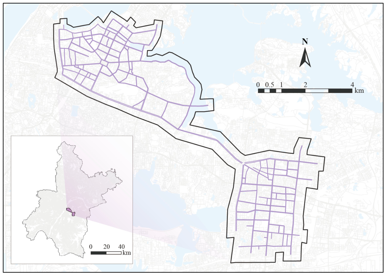
To cover diverse non-motorized travel scenarios and road environments, this study selected two functionally dense areas in the central urban area of Wuhan, together with their connecting roads, as shown in Figure 1. Wuhan is a major megacity in central China. By the end of 2024, its permanent resident population had exceeded 13.8 million [35]. The central urban area of Wuhan is characterized by high-density travel demand, mixed traffic between motorized and non-motorized users, prominent cyclist–pedestrian conflicts, discontinuous non-motorized lanes, long crossing detours, and frequent encroachment on road space.

The study area includes roads with established non-motorized lanes and different separation types, such as painted lines, guardrails, and green belts. These roads show clear differences in cycling space width, facility continuity, pavement condition, and traffic interference. Some road segments without dedicated non-motorized lanes often experience mixed traffic between motorized and non-motorized users, or between pedestrians and cyclists. In addition, the selected areas and their connecting roads cover diverse urban functions, including government offices, commercial centers, universities, and densely populated residential areas, as well as multiple road hierarchies and connectivity patterns. Therefore, the non-motorized lane environment in this area is highly diverse, providing a suitable sample for testing the applicability of the proposed framework under different road conditions.

2.2. Data Collection and Preprocessing

The dataset consisted of cycling-process data, urban spatial data, and training samples for computer-vision models. Cycling-process data were collected in June 2025 during weekday off-peak periods by seven volunteers riding freely within the predefined study area. Approximately 200 km of GPS trajectories and 14.5 h of usable first-person video were obtained. Videos were recorded at 1080 p and 30 fps, and GPS trajectories were recorded at approximately 1 Hz. Urban spatial data included OSM road networks and 2025 Baidu POIs, which were used for spatial registration, network matching, and indicator calculation. Key frames extracted from the cycling videos were used to construct training and validation samples for image classification, semantic segmentation, and object detection.

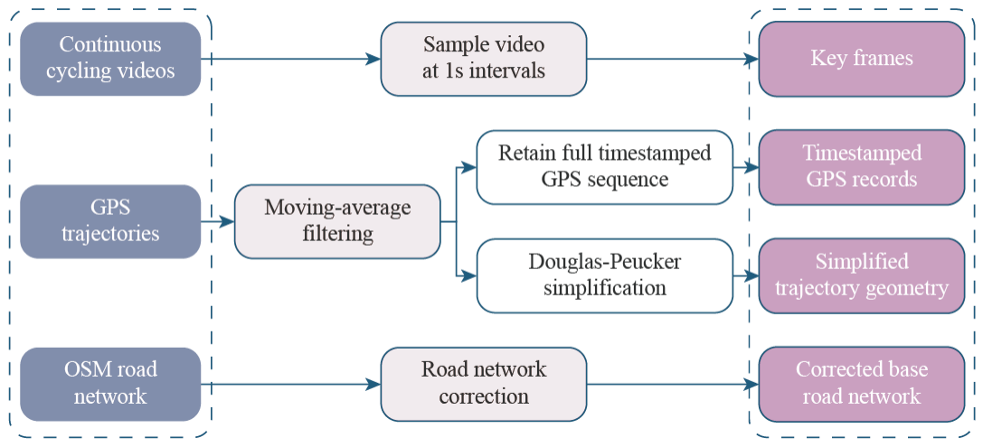
Preprocessing workflow, as shown in Figure 2, included video sampling, GPS filtering, trajectory simplification, road-network correction, and video–trajectory synchronization. Continuous videos were sampled at 1 s intervals, GPS trajectories were filtered to reduce short-term positioning noise, and simplified trajectory geometries were generated for map matching. Each sampled frame was linked to the nearest or interpolated GPS position according to timestamps, allowing visual-recognition results to be aggregated to road segments.

2.3. Overall Framework

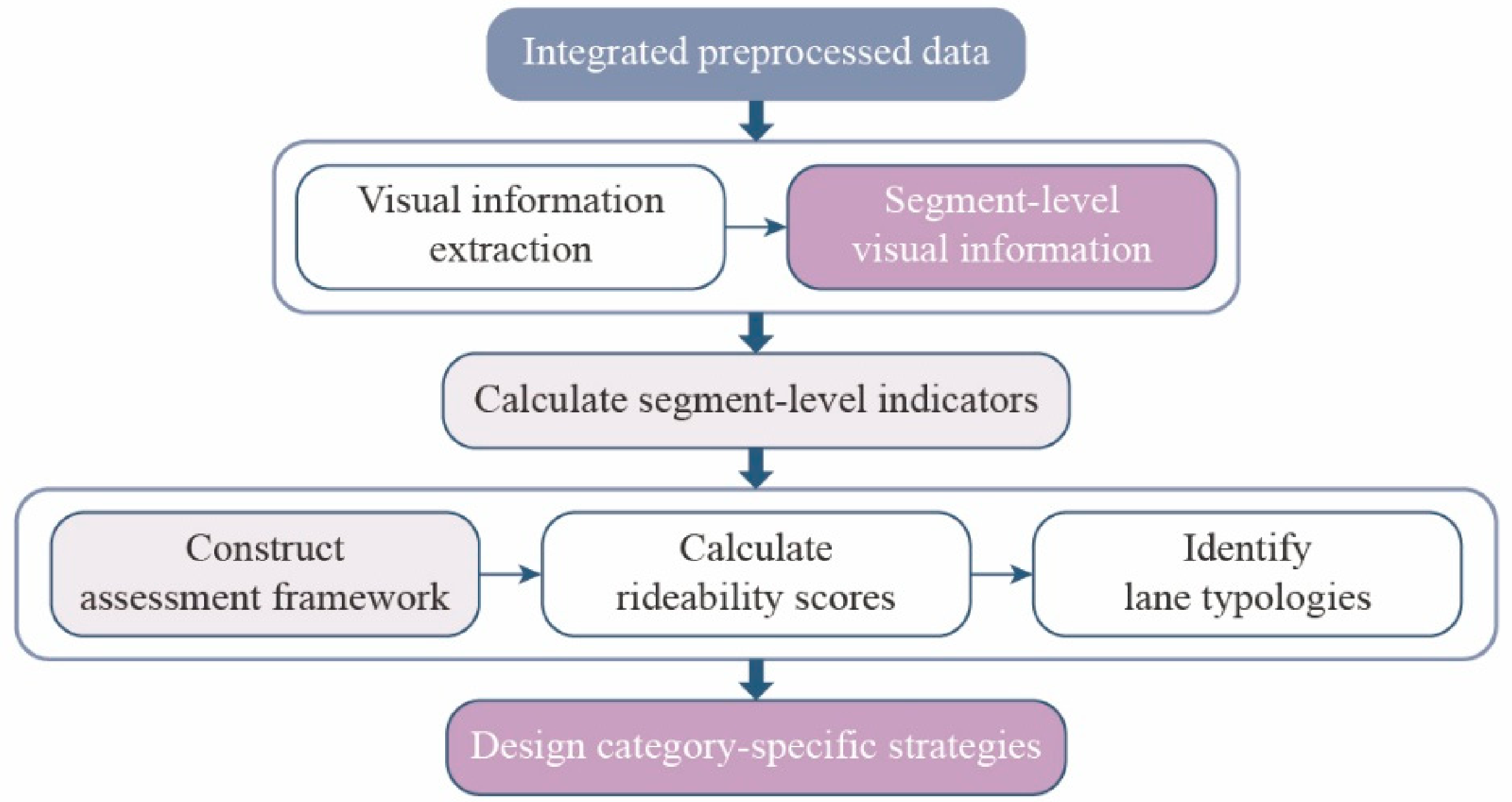
The overall workflow of the proposed framework is shown in Figure 3. It consists of three main stages: segment attribute extraction, rideability indicator construction, and rideability assessment with lane typology diagnosis.

In the segment-level attribute extraction stage, first-person cycling videos are processed using computer vision models to identify visual information related to the cycling environment, including lane conditions, facility characteristics, pavement conditions, and traffic disturbances. Meanwhile, cycling trajectories are matched to the corrected road network to determine the road segments corresponding to each riding record. Video frames and GPS trajectories are then synchronized by timestamps, and the frame-level recognition results are aggregated to the matched road segments. Through this process, visual observations collected during actual cycling are transformed into segment-level attributes.

In the rideability indicator construction stage, the extracted visual attributes are integrated with OSM road networks, public transport stops, POIs, and other spatial data. Based on these data, 16 segment-level indicators are constructed to describe the cycling environment of non-motorized lanes. These indicators provide the basis for evaluating both physical facility conditions and cyclists’ actual exposure to environmental and traffic disturbances.

In the rideability assessment and lane typology diagnosis stage, the 16 indicators are mapped to four assessment dimensions: safety, comfort, attractiveness, and accessibility. The entropy-weighted TOPSIS method is used to calculate the rideability score of each road segment under each dimension. Since individual dimension scores mainly reflect segment-level performance, Fuzzy C-means (FCM) clustering is further introduced to identify typical lane types with similar score structures and environmental characteristics. By combining dimension-specific scores with clustering results, the framework supports both quantitative assessment of individual road segments and diagnosis of common problem types in non-motorized lane environments.

2.4. Segment-Level Visual Information Extraction

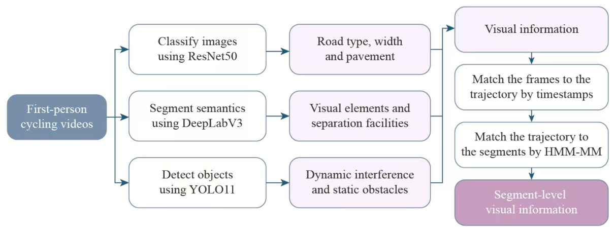
The workflow of segment-level visual information extraction is shown in Figure 4. To obtain different types of visual information, this study constructed three annotated datasets from the first-person cycling videos collected in the study area. These datasets were used for image classification, semantic segmentation, and object detection, respectively.

The image classification dataset was used to identify road type, lane-width category, and pavement type. Specifically, the road-type classification dataset contained 5502 annotated images, while the lane-width and pavement-type classification datasets were further constructed from images of non-motorized lanes. The semantic segmentation dataset was used to extract separation facilities and support the calculation of streetscape indicators, such as the green view index and sky openness index. This dataset contained 4700 annotated images. The object detection datasets were used to identify dynamic-disturbance targets and static-obstacle targets, containing 12,944 and 4100 images, respectively. Dynamic-disturbance targets included pedestrians, e-bikes, bicycles, cyclists, motor vehicles, and wrong-way non-motorized vehicles, while static-obstacle targets included manhole covers and roadblocks. In this study, e-bikes were defined as small electric two-wheelers commonly operating in or near non-motorized lanes, based on visible vehicle size, body structure, riding posture, and local traffic context. Motorcycles or motorized two-wheelers with clear motorcycle-like characteristics, as well as ambiguous samples that could not be reliably distinguished, were excluded during annotation and consistency checking.

For dataset annotation, different annotation rules were adopted for the three visual tasks. For image classification, each frame was labeled as a whole-image sample. Road type was classified into dedicated non-motorized lane, mixed motorized–non-motorized traffic, and mixed pedestrian–non-motorized traffic. Pavement type was classified into asphalt, concrete, and brick pavement. Non-motorized lane width was categorized as wide, moderate, or narrow based on field observations, riding-space appearance, and representative reference images prepared before annotation. For categories involving potential subjective judgment, multiple annotators independently reviewed the samples, and inconsistent labels were checked and revised. For semantic segmentation, this study did not perform lane-marking-level boundary mapping. Instead, the annotation focused on visible separation facilities and boundary elements between non-motorized lanes and adjacent motorized lanes or pedestrian spaces. The main annotated categories included separation barriers, green belts, and curbs. Polygon annotations were drawn along the visible outlines of target objects. Images with severe occlusion, unclear boundaries, or ambiguous categories were excluded from the effective training dataset. For object detection, bounding-box annotations were used to identify static obstacles and dynamic interference objects. Static obstacles included manhole covers and roadblocks, while dynamic interference objects included pedestrians, electric bicycles, bicycles, cyclists, motor vehicles, and wrong-way non-motorized vehicles. Wrong-way non-motorized vehicles were identified according to whether their travel direction was opposite to the designated direction of the current non-motorized lane. After annotation, manual consistency checks were conducted, and samples with incorrect labels, large bounding-box deviations, or unclear object boundaries were corrected or removed.

For object detection, frames were first extracted at a 2 s interval as candidate frames. This time-based interval was adopted because the cycling videos and GPS trajectories were synchronized through timestamps, allowing each detected object to be directly associated with the corresponding trajectory point and road segment. However, a purely time-based strategy may generate redundant observations when cyclists move slowly or wait at signalized intersections. Therefore, before calculating segment-level object densities, redundant candidate frames were further filtered according to trajectory displacement and riding speed. Frames collected during stationary or near-stationary periods were removed or merged, and consecutive frames with very small spatial displacement were not repeatedly counted. Thus, the 2 s interval served as a practical sampling interval for linking visual observations with trajectory data, while the resulting object-density indicators reflected observations after the removal of redundant frames.

The computer vision models were implemented in Python 3.10 using PyTorch 2.4.1. ResNet50 and DeepLabv3+ were implemented in the PyTorch framework for image classification and semantic segmentation, respectively. The object detection task was implemented using YOLO11m with the Ultralytics YOLO package version 8.3.0 [36,37,38]. These models have mature pretrained architectures and have been widely used in their corresponding tasks. The validation results of the trained models on the test sets are shown in

Table 1. Performance validation of computer vision models.

Model	Task	Target Category	Accuracy (%)	Precision (%)	Recall (%)	mIoU (%)	mAP@0.5 (%)
ResNet50	Classification	Road type	97	—	—	—	—
		Road width	91	—	—	—	—
		Pavement	92	—	—	—	—
		Mean	93.3	—	—	—	—
DeepLabv3+	Segmentation	Physical separation	81.4	72.4	68.5	57.2	—
		Greenery	83.6	78.1	73.9	61.8	—
		Curb	79.3	71	66.7	55.9	—
		Mean	81.4	73.8	69.7	58.3	—
YOLO11	Dynamic object detection	Pedestrian	—	83.0	78.0	—	81.0
		E-bike	—	82.0	78.0	—	79.0
		Bicycle	—	84.0	79.0	—	86.0
		Cyclist	—	80.0	75.0	—	76.0
		Car	—	88.0	85.0	—	90.0
		Wrong-way rider	—	78.0	75.0	—	76.0
		Mean	—	83.0	78.0	—	81.0
	Static obstacle detection	Manhole cover	—	79.0	74.0	—	76.0
		Roadblock	—	81.0	75.0	—	78.0
		Mean	—	80.0	75.0	—	77.0

Note. “—” indicates that the metric is not applicable to the corresponding task.

. The classification accuracy ranged from 0.91 to 0.97. For separation-facility semantic segmentation, the mean accuracy and mean intersection over union (mIoU) were 81.4% and 58.3%, respectively. For object detection, the mAP@0.5 values of dynamic object detection and static obstacle detection were 0.81 and 0.77, respectively.

After frame-level visual recognition, the recognition results were further associated with specific road segments. Using the simplified trajectory geometry and the corrected base road network obtained from the preprocessing stage, a Hidden Markov Model (HMM)-based map-matching method was applied to match trajectory points to the base road network [39,40]. After the correspondence among video frames, trajectory points, and road segments was established, each frame-level visual recognition result was linked to its corresponding road segment and converted into segment-level statistics. In this way, frame-level visual recognition results were aggregated into segment-level basic data for subsequent indicator calculation.

2.5. Construction of Multidimensional Indicator System

2.5.1. Objective Indicator System

To quantify the environmental information of non-motorized lanes extracted from multi-source data, this study constructed 16 objective indicators.

Table 2. Objective measurement indicators for non-motorized lanes.

Category	Indicator	Quantification
Visual ratio indicators	Green view index	${\mathrm{A}}_{\mathrm{g}\mathrm{r}\mathrm{e}\mathrm{e}\mathrm{n}}/{\mathrm{A}}_{\mathrm{t}\mathrm{o}\mathrm{t}\mathrm{a}\mathrm{l}}$
	Sky openness index	${\mathrm{A}}_{\mathrm{s}\mathrm{k}\mathrm{y}}/{\mathrm{A}}_{\mathrm{t}\mathrm{o}\mathrm{t}\mathrm{a}\mathrm{l}}$
	Interface enclosure index	${\mathrm{A}}_{\mathrm{b}\mathrm{u}\mathrm{i}\mathrm{l}\mathrm{d}}/{\mathrm{A}}_{\mathrm{t}\mathrm{o}\mathrm{t}\mathrm{a}\mathrm{l}}$
	Motorization index	${\mathrm{A}}_{\mathrm{v}\mathrm{e}\mathrm{h}\mathrm{i}\mathrm{c}\mathrm{l}\mathrm{e}}/{\mathrm{A}}_{\mathrm{t}\mathrm{o}\mathrm{t}\mathrm{a}\mathrm{l}}$
Density indicators	Pedestrian density	${\mathrm{N}}_{\mathrm{p}\mathrm{e}\mathrm{d}\mathrm{e}\mathrm{s}\mathrm{t}\mathrm{r}\mathrm{i}\mathrm{a}\mathrm{n}}/\mathrm{L}$
	Wrong-way rider density	${\mathrm{N}}_{\mathrm{r}\mathrm{e}\mathrm{t}\mathrm{r}\mathrm{o}\mathrm{g}\mathrm{r}\mathrm{a}\mathrm{d}\mathrm{e}}/\mathrm{L}$
	Manhole exposure density	${\mathrm{N}}_{\mathrm{m}\mathrm{a}\mathrm{n}\mathrm{h}\mathrm{o}\mathrm{l}\mathrm{e}}/\mathrm{L}$
	Roadblock exposure density	${\mathrm{N}}_{\mathrm{r}\mathrm{o}\mathrm{a}\mathrm{d}\mathrm{b}\mathrm{l}\mathrm{o}\mathrm{c}\mathrm{k}}/\mathrm{L}$
GIS-based spatial indicators	Parcel access-point density	${\mathrm{N}}_{\mathrm{a}\mathrm{c}\mathrm{c}\mathrm{e}\mathrm{s}\mathrm{s}}/\mathrm{L}$
	Road network density	GIS Grid Statistics
	Public transport density	${(\mathrm{N}}_{\mathrm{b}\mathrm{u}\mathrm{s}}+4·{\mathrm{N}}_{\mathrm{s}\mathrm{u}\mathrm{b}})/\mathrm{L}$
	Crossing circuity factor	$\sum {(\mathrm{R}}_{\mathrm{i}}·{\mathrm{w}}_{\mathrm{i}})/\mathrm{n}$
Ordinal scoring indicators	Separation (motorized)	Scoring
	Separation (pedestrian)	Scoring
	Pavement smoothness	Scoring
	Lane width	Scoring

summarizes the category, name, and quantification method of each indicator, and the meanings of the variables used in the formulas are provided in

Table 3. Definitions of variables used in the indicator formulas.

Variable	Definition
${\mathrm{A}}_{\mathrm{g}\mathrm{r}\mathrm{e}\mathrm{e}\mathrm{n}}$	Pixel area of greenery in the image
${\mathrm{A}}_{\mathrm{s}\mathrm{k}\mathrm{y}}$	Pixel area of sky in the image
${\mathrm{A}}_{\mathrm{b}\mathrm{u}\mathrm{i}\mathrm{l}\mathrm{d}}$	Pixel area of buildings and walls in the image
${\mathrm{A}}_{\mathrm{v}\mathrm{e}\mathrm{h}\mathrm{i}\mathrm{c}\mathrm{l}\mathrm{e}}$	Pixel area occupied by motorized vehicles in the image
${\mathrm{A}}_{\mathrm{t}\mathrm{o}\mathrm{t}\mathrm{a}\mathrm{l}}$	Effective pixel area of the image used for visual-ratio calculation
${\mathrm{N}}_{\mathrm{p}\mathrm{e}\mathrm{d}\mathrm{e}\mathrm{s}\mathrm{t}\mathrm{r}\mathrm{i}\mathrm{a}\mathrm{n}}$	Number of pedestrians detected within a road segment
${\mathrm{N}}_{\mathrm{r}\mathrm{e}\mathrm{t}\mathrm{r}\mathrm{o}\mathrm{g}\mathrm{r}\mathrm{a}\mathrm{d}\mathrm{e}}$	Number of wrong-way riders detected within a road segment
${\mathrm{N}}_{\mathrm{m}\mathrm{a}\mathrm{n}\mathrm{h}\mathrm{o}\mathrm{l}\mathrm{e}}$	Number of visible manhole covers detected within a road segment
${\mathrm{N}}_{\mathrm{r}\mathrm{o}\mathrm{a}\mathrm{d}\mathrm{b}\mathrm{l}\mathrm{o}\mathrm{c}\mathrm{k}}$	Number of roadblocks or physical blocks detected within a road segment
${\mathrm{N}}_{\mathrm{a}\mathrm{c}\mathrm{c}\mathrm{e}\mathrm{s}\mathrm{s}}$	Number of parcel access points within a road segment
${\mathrm{N}}_{\mathrm{b}\mathrm{u}\mathrm{s}}$	Number of bus stops associated with a road segment
${\mathrm{N}}_{\mathrm{s}\mathrm{u}\mathrm{b}}$	Number of subway stations associated with a road segment
$\mathrm{L}$	Length of the corresponding road segment
${\mathrm{R}}_{\mathrm{i}}$	Crossing circuity factor of the $\mathrm{i}\mathrm{t}\mathrm{h}$ parcel access point
${\mathrm{w}}_{\mathrm{i}}$	Weight assigned to the $\mathrm{i}\mathrm{t}\mathrm{h}$ parcel access point according to adjacent POI type
$\mathrm{n}$	Number of parcel access points within the road segment

.

Overall, the indicators in this study were organized into four groups according to data source and calculation logic. The first group consists of visual ratio indicators, including the green view index, sky openness index, interface enclosure index, and motorization index. These indicators describe the proportions of greenery, sky, buildings and walls, and motorized vehicles in the visual field, respectively, and were calculated as the ratio of the corresponding pixel or object area to the effective image area.

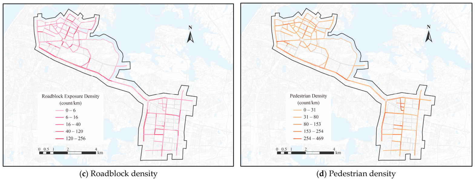
The second group consists of density indicators, including pedestrian density, wrong-way rider density, manhole exposure density, roadblock exposure density, and parcel access-point density. These indicators, respectively, describe the number of pedestrians, riders moving against traffic, visible manhole covers, roadblocks or physical blocks, and parcel access points along each road segment. They were calculated by counting the corresponding objects or access points within a road segment and standardizing the counts by segment length.

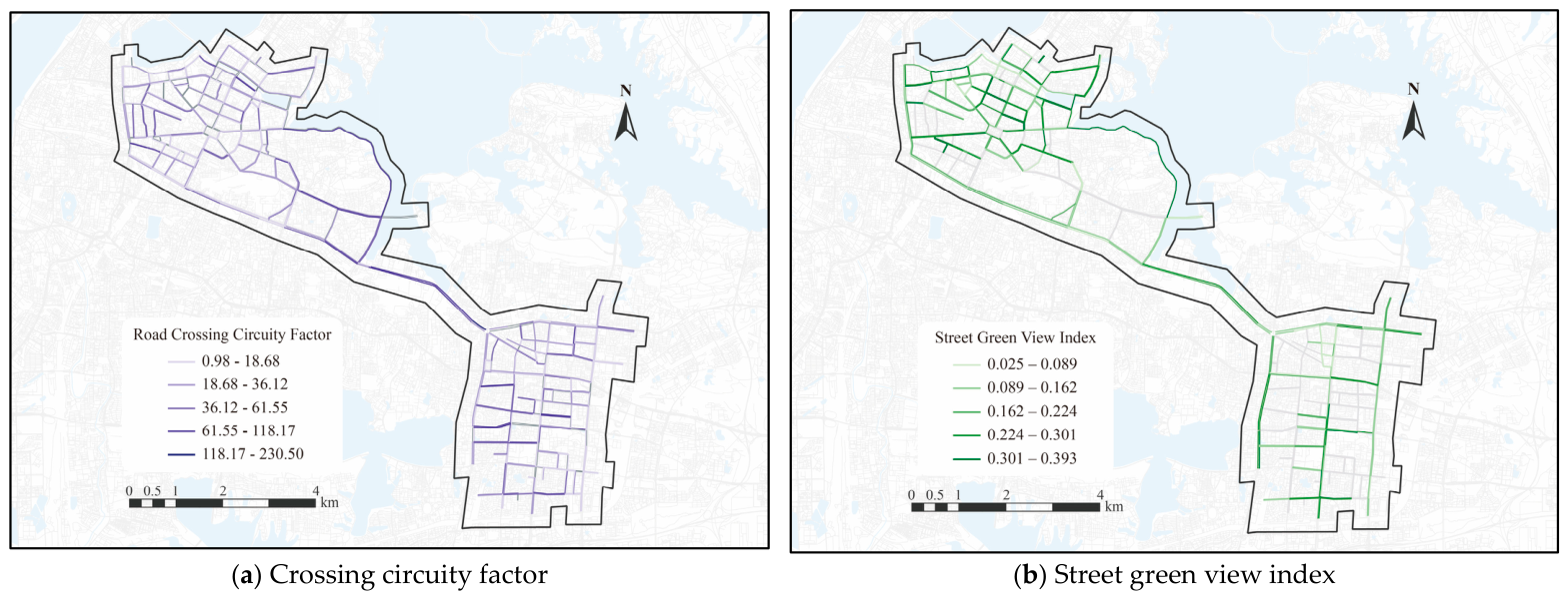
The third group consists of GIS-based spatial indicators, including road network density, public transport density, and the crossing circuity factor. Road network density was calculated as the total road length per unit area, public transport density was calculated as the weighted density of bus and subway stations, and the crossing circuity factor was calculated as the ratio of legal crossing path length to road width. These indicators were used to characterize network connectivity, public transport accessibility, and crossing detour cost.

The fourth group consists of ordinal scoring indicators, including motorized–non-motorized separation, pedestrian–non-motorized separation, pavement smoothness, and lane width. These indicators describe physical or visual separation from motorized lanes and sidewalks, the surface material and smoothness of the lane, and the physical width capacity of the riding space. Since these attributes are categorical and difficult to represent directly using continuous numerical values, ordinal scores were assigned according to relevant planning standards [41,42], the protective strength of facilities, and differences in pavement smoothness. The scoring criteria are described in Supplementary Note S1.

2.5.2. Calculation of Crossing Circuity Factor

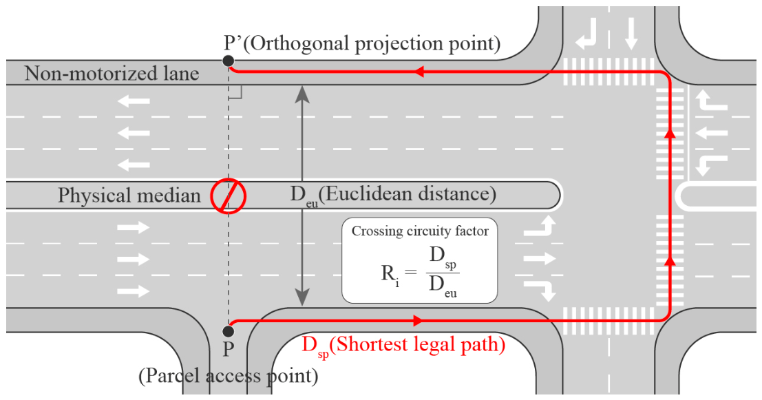
Non-motorized users frequently need to cross streets, and the physical distance required to complete a legal crossing directly affects cycling efficiency. To quantitatively measure this detour cost, this study formulated a spatial indicator, the crossing circuity factor, based on parcel access points. The geometric and topological calculation logic is illustrated in Figure 5.

To reflect the actual crossing demand generated by urban functions, a weight coefficient ($w_i$) is assigned to each access point based on adjacent point of interest types: 1.5 for transit stations and schools, 1.3 for commercial facilities, and 1.0 for general residential or leisure areas. Finally, the segment-level crossing circuity factor is aggregated as the weighted average:

$$R_{road}={\displaystyle \frac{{\sum }_{i=1}^n{R}_i\ast w_i}{n}}$$

(1)

where $n$ is the total number of access points on the segment. A higher $R_{road}$ value indicates a greater geometric detour penalty and lower crossing convenience.

2.6. Rideability Assessment and Typology Diagnosis

2.6.1. Rideability Assessment Using Entropy-Weighted TOPSIS

After constructing the 16 rideability indicators, this study further mapped each indicator to the corresponding assessment dimension. The dimension classification mainly refers to the requirements for safe travel, riding comfort, environmental quality, and spatial accessibility in urban slow-traffic planning and design, and also incorporates commonly used assessment frameworks in existing rideability studies. 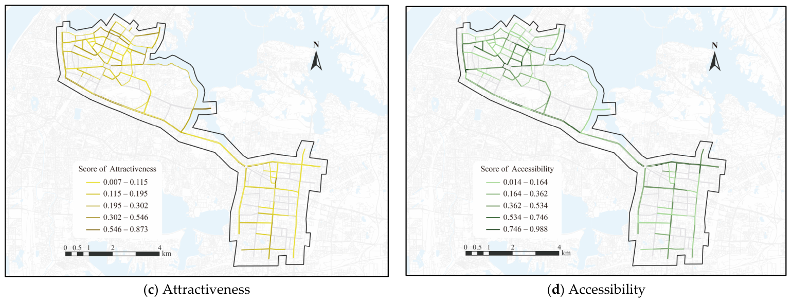Finally, the rideability of non-motorized lanes was organized into four core dimensions: safety, comfort, attractiveness, and accessibility [43,44]. Among them, safety focuses on factors that may generate conflicts or risks during cycling; comfort focuses on spatial oppression and traffic disturbances during cycling; attractiveness focuses on the visual environmental quality perceived by cyclists; and accessibility focuses on the degree of connection between road segments and the road network, public transport, and surrounding functional spaces. The specific indicators corresponding to each dimension and their impact polarities are shown in

Table 4. Indicator system for rideability assessment of non-motorized lanes.

Dimension	Indicator	Direction
Safety	Separation between motorized and non-motorized traffic	Positive
	Separation between pedestrians and non-motorized traffic	Positive
	Pavement smoothness	Positive
	Lane width category	Positive
	Motorization index	Negative
	Wrong-way non-motorized vehicle density	Negative
	Pedestrian density	Negative
Comfort	Interface enclosure index	Negative
	Manhole exposure density	Negative
	Roadblock exposure density	Negative
	Parcel access-point density	Negative
Attractiveness	Green view index	Positive
	Sky openness index	Positive
Accessibility	Crossing circuity factor	Negative
	Road network density	Positive
	Public transport stop density	Positive

. Positive indicators, such as the green view index, enhance the cycling experience, meaning that higher values indicate better performance. Negative indicators, such as pedestrian density, have the opposite effect.

It should be noted that some indicators may simultaneously affect multiple perceptual dimensions of cycling. For example, pavement condition may influence both riding comfort and riding safety, while lane width is related not only to riding comfort but also to the risk of motorized–non-motorized and pedestrian–cyclist conflicts. To avoid repeated calculation of the same indicator across multiple dimensions, this study assigned each indicator to the assessment dimension that it most directly represents.

To quantify the performance of non-motorized lanes across the four assessment dimensions, this study used the entropy-weighted TOPSIS method to calculate the score of each dimension [45,46]. The entropy weighting method was selected because the indicators in this study are derived from objective observational data, including road facilities, visual perception, traffic interference, and spatial network characteristics. Compared with subjective weighting methods such as the Analytic Hierarchy Process (AHP), which rely on expert judgment and pairwise comparison matrices, the entropy weighting method determines indicator weights according to the dispersion of indicator values among sample road segments. This helps reduce the influence of subjective judgment and is more suitable for a replicable segment-level assessment based on multi-source cycling and spatial data. Specifically, the greater the variation in an indicator across road segments, the more information it provides for distinguishing differences among segments, and the higher its weight. Therefore, the entropy-derived weights in this study reflect the information contribution and discriminatory power of each indicator within the current sample. After the weights were determined, the TOPSIS method was used to construct the positive ideal solution and the negative ideal solution based on the weighted indicator matrix. The assessment score was then obtained by calculating the relative distance between each road segment and the two ideal solutions. In this study, the entropy-weighted TOPSIS method was applied separately within the four dimensions of safety, comfort, attractiveness, and accessibility to obtain the multidimensional rideability scores of each road segment. The specific calculation process for each dimension is as follows.

First, to eliminate dimensional differences among indicators and reduce the influence of extreme outliers, a quantile-based normalization method was applied. The 5th and 95th percentiles of each indicator were used as the lower and upper boundaries. For positive indicators, the normalization is defined as:

$$z_{ij} = \left\{\begin{array}{l}0, x_{ij} \le Q_{0.05}\\ {\displaystyle \frac{x_{ij} - Q_{0.05}}{Q_{0.95} - Q_{0.05}}}, Q_{0.05} < x_{ij} < Q_{0.95}\\ 1, Q_{0.95} \le x_{ij}\end{array}\right.$$

(2)

For negative indicators, the normalization is:

$$z_{ij} = \left\{\begin{array}{l}1, x_{ij} \le Q_{0.05}\\ {\displaystyle \frac{Q_{0.95} - x_{ij}}{Q_{0.95} - Q_{0.05}}}, Q_{0.05} < x_{ij} < Q_{0.95}\\ 0, Q_{0.95} \le x_{ij}\end{array}\right.$$

(3)

where $x_{ij}$ is the original value of the $j$-th indicator for the $i$-th road segment, and $z_{ij}$ is the standardized value.

Subsequently, the entropy weight method was applied to objectively determine the weight of each indicator based on its information dispersion. The information entropy $e_j$ and the final weight $w_j$ were calculated as follows:

$$p_{ij}={\displaystyle \frac{z_{ij}}{{\sum }_{i=1}^m{z}_{ij}}}$$

(4)

$$e_j=-{\displaystyle \frac{1}{ln\left(m\right)}}{\sum }_{i=1}^m{p}_{ij}\ln {(p}_{ij}+ϵ)$$

(5)

$$w_j={\displaystyle \frac{1 - e_j}{{\sum }_{j=1}^{n}1 - e_j}}$$

(6)

where $m$ is the total number of evaluated segments, $n$ is the number of indicators within the current dimension, and$ϵ$ is an infinitesimally small constant to prevent zero-value logarithms.

Finally, the TOPSIS method calculates the weighted Euclidean distance from each segment to the positive ideal solution ($Z^{+}$) and the negative ideal solution ($Z^{ - }$). The distances $D_i^{+}$ and $D_i^{ - }$ are given by:

$$D_i^{+} = \sqrt{{\sum }_{j=1}^n{w}_j{\left(Z_j^{+} - z_{ij}\right)}^2}$$

(7)

$$D_i^{-}=\sqrt{{\sum }_{j=1}^n{w}_j{\left(Z_j^{-}- z_{ij}\right)}^2}$$

(8)

The comprehensive dimension score ${\mathrm{S}}_{\mathrm{i}}$ for the $i$-th road segment is then computed as:

$$S_i={\displaystyle \frac{D_i^{ - }}{D_i^{+}+ D_i^{ - }}}$$

(9)

A higher $S_i$ value (closer to 1) indicates that the segment’s performance in that specific dimension is closer to the ideal state.

2.6.2. Segment Typology Diagnosis Using FCM Clustering

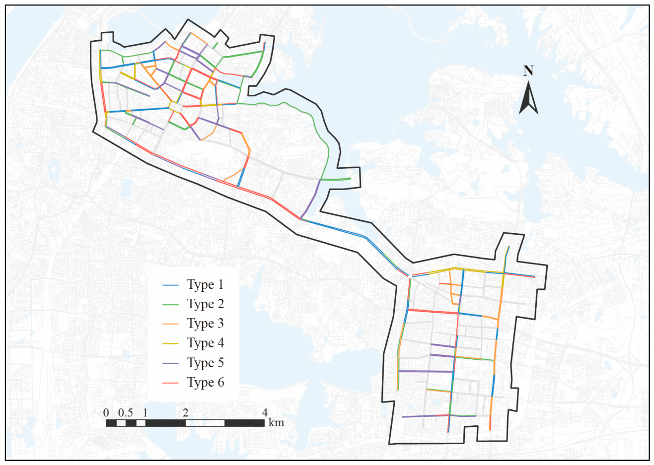
The environmental characteristics of non-motorized lanes often vary continuously in space, and the boundaries between different segment types are not absolutely clear. Therefore, this study adopts fuzzy C-means (FCM) clustering to classify road segments. Unlike hard clustering methods such as K-means, FCM allows the same segment to approach multiple clusters with different membership degrees, thereby avoiding the forced assignment of transitional segments to a single category and better reflecting the gradual and mixed characteristics of segment-level environments. Referring to the commonly used six-level interpretation framework in bicycle level-of-service studies, the number of clusters was set to $k=6$ [47,48]. The algorithm minimizes the objective function $J$ by iteratively updating the membership matrix and cluster centers:

$$J = {\displaystyle \sum _{i=1}^n}{\displaystyle \sum _{j=1}^k}{u}_{ij}^m{‖x_i - c_j‖}^2$$

(10)

where $n$ is the number of segments, $x_i$ represents the four-dimensional score vector of the $i$-th segment, $c_j$ is the $j$-th cluster center, $u_{ij}$ denotes the membership degree of segment $i$ to cluster $j$, $k$ is the predefined number of clusters, and $m$ is the fuzziness exponent, which is set to $m=2$ [49,50,51] in this study. The algorithm iteratively updates the membership matrix and cluster centers so that the objective function $J$ gradually decreases. The iteration terminates when the change in the membership matrix between two consecutive iterations is smaller than the convergence threshold $\epsilon$, or when the maximum number of iterations is reached. In this study, $\epsilon =1\times {10}^{ - 4}$, and the maximum number of iterations is set to 300. Finally, each road segment is assigned to the corresponding type according to its maximum membership degree, while its membership degrees to other types are also retained.

3. Results

3.1. Extraction Results of Street Indicators

This section presents the visualization results of four representative indicators, namely the crossing circuity factor, street green view index, roadblock exposure density, and pedestrian density, as shown in Figure 6. These four indicators, respectively, represent spatial network topology, street-level visual perception, static traffic interference, and dynamic traffic interference, and therefore provide a representative description of the micro-environment of non-motorized lanes.

The crossing circuity factor shows clear differences across road classes. Lower values are mainly observed on local streets and sub-arterial roads with denser surrounding networks, whereas higher values are concentrated along expressways and major arterial corridors where crossing opportunities are limited. The street green view index is higher along segments with continuous roadside greenery and lower along high-intensity traffic corridors and enclosed built-up streets. Roadblock exposure density shows localized concentrations, indicating that static obstacles are unevenly distributed rather than uniformly present across the network. Pedestrian density is higher around commercial, residential, and public-service areas, reflecting stronger pedestrian–cyclist interaction in functionally dense urban spaces.

Overall, the four indicators demonstrate that the proposed extraction workflow can capture heterogeneous micro-environmental conditions at the road-segment scale. These segment-level indicators provide the basis for the subsequent multidimensional rideability assessment.

3.2. Rideability Assessment

Table 5. Descriptive statistics and entropy weights of the rideability indicators.

Dimension	Indicator	95% Quantile	5% Quantile	Mean	Weight
Safety	Separation motorized	1	0.5	0.81	0.24
	Separation pedestrians	1	0.5	0.73	0.19
	Pavement smoothness	1	0.7	0.90	0.12
	Lane width category	1	0.3	0.58	0.24
	Motorization index	0.07	0.02	0.03	0.08
	Wrong-way density	17	0	5	0.06
	Pedestrian density	36	0	12	0.07
Comfort	Interface enclosure index	0.76	0.55	0.65	0.31
	Manhole exposure density	15	1	6	0.22
	Roadblock exposure density	11	0	2	0.19
	Parcel access-point density	4	0	2	0.28
Attractiveness	Green view index	0.31	0.08	0.19	0.63
	Sky openness index	0.11	0.01	0.05	0.37
Accessibility	Crossing circuity factor	48.20	7.97	21.44	0.22
	Road network density	45.40	18.14	32.95	0.24
	Public transport stop density	6.47	0	2.63	0.54

reports the descriptive statistics and entropy weights of the 16 indicators. In the safety dimension, motorized–non-motorized separation and lane width obtained the highest weights, indicating that facility protection and cycling-space provision were the main factors differentiating segment-level safety. In the comfort dimension, interface enclosure and parcel access-point density contributed strongly to score variation, suggesting that spatial oppression and boundary disturbance were important sources of comfort differences. In the attractiveness dimension, the green view index had a higher weight than sky openness, indicating that greenery was the dominant visual factor distinguishing segment attractiveness. In the accessibility dimension, public transport stop density had the largest weight, followed by road network density and crossing circuity factor, reflecting the uneven distribution of multimodal connectivity and crossing convenience across the study area.

Figure 7 shows the spatial distribution of rideability scores under the four dimensions. Safety scores are higher on segments with stronger separation facilities and wider cycling space, while lower values are more common on roads with mixed traffic, weak separation, or stronger traffic interference. Comfort scores show a different spatial pattern and are more closely associated with interface enclosure, static obstacles, and access-point disturbance. Attractiveness scores are concentrated on segments with continuous greenery and open visual fields, whereas expressway side roads and high-intensity traffic corridors tend to have lower visual quality. Accessibility scores are higher on arterial roads and some secondary roads with denser network connections and better public transport access, while isolated branches, scenic roads, and expressway-side segments often score lower because of weaker connectivity or higher crossing detour costs.

These results show clear divergence among the four dimensions. Segments with high accessibility do not necessarily have high safety or attractiveness, and visually favorable segments may still have weak network connectivity. Therefore, the dimension-specific assessment provides a basis for identifying different types of strengths and deficiencies before clustering analysis.

3.3. Typologies of Non-Motorized Lanes and Their Relationship with Road Hierarchy

Based on the four dimension-specific scores, FCM clustering classified all non-motorized lane segments into six typologies.

Table 6. Statistical characteristics of lane typologies.

Type	Safety	Comfort	Attractiveness	Accessibility
1	0.706	0.620	0.142	0.386
2	0.584	0.777	0.202	0.121
3	0.638	0.442	0.101	0.086
4	0.559	0.508	0.145	0.698
5	0.324	0.642	0.187	0.088
6	0.338	0.586	0.154	0.443

reports the mean scores of each typology, and Figure 8 shows their spatial distribution. The six types represent different combinations of safety, comfort, attractiveness, and accessibility rather than a simple high-to-low quality ranking.

Type 1 is safety-dominant, with the highest safety score and relatively good comfort, indicating stronger facility separation and more stable riding conditions. Type 2 is comfort- and attractiveness-oriented but has low accessibility, suggesting favorable local riding environments with limited network connection. Type 3 shows relatively weak comfort, attractiveness, and accessibility, representing segments with limited overall rideability despite moderate safety. Type 4 is accessibility-dominant, with the highest accessibility score but only moderate safety and comfort. Type 5 has relatively high comfort and attractiveness but low safety and accessibility, indicating visually acceptable local environments with insufficient protection and connectivity. Type 6 has moderate accessibility but low safety, reflecting a mismatch between transport function and cycling-infrastructure provision.

The length-based cross-tabulation in

Table 7. Distribution of lane typologies by length proportion within each road hierarchy.

Road Hierarchy	Type 1	Type 2	Type 3	Type 4	Type 5	Type 6
Express	24.0%	8.0%	38.2%	7.0%	2.0%	20.9%
Arterial	19.6%	12.0%	13.1%	14.2%	9.5%	31.6%
Sub-arterial	22.7%	21.4%	6.8%	8.0%	23.6%	17.4%
Local	0.0%	22.5%	32.2%	6.1%	36.5%	2.6%

shows that lane typologies vary substantially by road hierarchy. Express-road-related segments are dominated by Type 3, followed by Type 1 and Type 6, indicating a combination of structural separation and limited comfort, attractiveness, or accessibility. Arterial roads are dominated by Type 6, while Type 1 and Type 4 also account for notable proportions, reflecting the coexistence of strong transport connectivity and uneven cycling-environment quality. Sub-arterial roads show the most balanced typological composition, with Type 5, Type 1, Type 2, and Type 6 all occupying considerable proportions. Local streets are dominated by Type 5 and Type 3, while Type 1 is absent, suggesting that local streets rarely provide safety-dominant, fully separated non-motorized lane environments.

Overall, the typology results indicate that road hierarchy is closely related to rideability structure, but it does not determine cycling-environment quality by itself. The same road class may contain multiple typologies, and the same typology may appear across different road classes. This result provides the empirical basis for the road-class sensitivity analysis and type-specific discussion in Section 4.

4. Discussion

4.1. Multidimensional Trade-Offs in Non-Motorized Lane Rideability

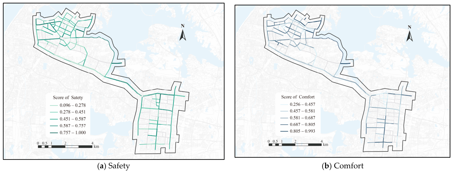
Previous rideability studies have emphasized the importance of infrastructure provision, land-use accessibility, network connectivity, traffic safety, comfort, and visual attractiveness in assessing cycling environments [11,15,17,18,43,44]. For example, urban Bikeability Index studies have used built-environment and cyclist-preference indicators to support bicycle infrastructure prioritization, while recent reviews show that Bicycle Level of Service, Bikeability Index, Bicycle Safety Index, and roughness- or comfort-related measures remain major approaches for evaluating bicycle environments. The present results confirm the relevance of these dimensions, but they further show that these dimensions do not necessarily improve simultaneously at the road-segment scale.

The results of this study show that the rideability of non-motorized lanes cannot be adequately summarized by a single overall score. Instead, it is shaped by the multidimensional combination of safety, comfort, attractiveness, and accessibility. In the study area, different segments show inconsistent performance across these four dimensions. Some segments have good network connectivity and public transport access but insufficient safety, whereas others have favorable visual environments and relatively low riding disturbance but weak connections with the urban road network and public transport system. This indicates that neither the mere presence of a non-motorized lane nor a single composite assessment score is sufficient for accurately judging cycling environmental quality. For non-motorized lanes, it is more important to identify structural differences among dimensions and further explain the traffic operation, facility conditions, and surrounding environmental factors behind these differences.

One notable finding is that some highly accessible segments do not necessarily provide high safety. These segments are mainly located along arterial roads, commercial centers, transport hubs, and their surrounding areas. Because these areas usually have high road-network density, concentrated public transport stops, and dense surrounding destinations and entrances, cyclists can access different urban functional spaces relatively easily, resulting in good accessibility performance. However, these segments also tend to carry stronger motorized traffic functions, more complex intersection organization, and more frequent pedestrian crossing, motor-vehicle interference, temporary occupation, and wrong-way non-motorized riding. Under such conditions, multiple conflicts caused by high-intensity traffic activity can directly weaken cycling safety. Even when basic non-motorized travel space exists, cyclists may still be exposed to relatively high operational risks. Therefore, high accessibility does not necessarily imply a good rideability environment. This finding qualifies accessibility-oriented rideability studies by showing that network connectivity, public transport access, and destination concentration may improve access while simultaneously increasing exposure to operational conflicts in dense mixed-traffic areas [23,24,26].

In contrast, some segments with high comfort or attractiveness may still suffer from insufficient accessibility. These segments usually include greenways, scenic roads, local branches, and living streets with relatively good environmental conditions. They often have better greenery, lower spatial oppression, and less motorized traffic interference, and can therefore provide a more favorable visual experience and riding comfort. However, because these roads are sometimes located at the edge of the road network or mainly serve recreational functions, their connections with the main urban road network, public transport stops, and surrounding high-intensity functional spaces may be weak. This suggests that a visually pleasant or comfortable cycling space does not necessarily have high overall rideability. Recreational cycling spaces and daily commuting cycling spaces have different functional orientations and should not be interpreted using the same assessment logic.

4.2. Contribution of Cycling-Process Data to Segment-Level Diagnosis

Previous studies have demonstrated that street-view imagery and computer vision can improve the automatic measurement of cycling environments by extracting visual indicators at fine spatial scales [19,20,21,22]. Trajectory-based rideability studies have also strengthened street-level assessment by linking observed cycling behavior with built-environment characteristics [23,24,25,26]. However, these two lines of research usually emphasize either static environmental representation or aggregate cycling-use patterns. They are less able to capture temporary and process-specific disturbances encountered during actual riding, such as pedestrian intrusion, wrong-way riders, roadblocks, and temporary occupation, or to explain why a specific road segment performs poorly. This gap is directly related to the segment-level diagnostic objective of this study.

To address this gap, this study integrates first-person cycling videos, GPS trajectories, road networks, and POI data within a unified road-segment-based analytical framework. Frame-level visual recognition results are linked to specific road segments through temporal synchronization and map matching, so that observations recorded during actual cycling can be converted into comparable segment-level attributes. Through this integration, dynamic disturbances, facility attributes, visual environments, and spatial accessibility are represented within the same analytical unit, making cross-dimensional comparison and diagnosis possible. In particular, dynamic phenomena such as pedestrian intrusion, wrong-way non-motorized vehicles, roadblocks, and temporary occupation are no longer treated as isolated video observations, but are quantified as segment-level disturbance characteristics. As a result, the assessment results can not only indicate which segments perform poorly, but also help explain whether low performance is more likely to result from traffic conflicts, spatial oppression, facility discontinuity, or insufficient network connection.

Therefore, the proposed framework not only confirms the value of visual and trajectory data emphasized in previous rideability studies, but also extends them from environmental measurement and cycling-behavior description toward road-segment-level problem diagnosis.

4.3. Road-Class Sensitivity Analysis

Road hierarchy has long been recognized as an important factor affecting cyclists’ perceived safety and traffic stress, because it is closely related to motor-vehicle speed, traffic volume, lane configuration, intersection complexity, and the need for physical separation. The Level of Traffic Stress (LTS) literature further emphasizes that bicycle network suitability depends not only on the existence of cycling facilities, but also on whether cyclists can travel through connected low-stress links without being forced onto high-stress roads [52,53]. Therefore, road hierarchy may affect how segment-level safety scores should be interpreted. To examine this issue, this study conducted a road-class sensitivity analysis using the safety dimension as an example.

The original safety scores calculated under the unified citywide entropy-weighted TOPSIS framework were first retained as the main assessment results. Then, the scores were recalculated within each road hierarchy using the same entropy-weighted TOPSIS procedure. Because the normalization ranges, entropy weights, and positive and negative ideal solutions in TOPSIS are recalculated within each road class, the raw TOPSIS scores obtained from road-class-specific calculations are not suitable for direct comparison across road hierarchies. Therefore, this study did not directly compare the raw scores. Instead, the score of each road segment was converted into a percentile ranking within its corresponding road hierarchy, and the two sets of ranking results were further compared. This study used three indicators to compare the two sets of ranking results, as shown in

Table 8. Road-class sensitivity analysis of safety rankings.

Road Hierarchy	Spearman Correlation	Mean Absolute Percentile-Rank Change	Same or Adjacent Quartile (%)
Express	0.955	0.051	100
Arterial	0.364	0.252	76.1
Sub-arterial	0.933	0.079	100
Local	0.962	0.043	100

. The Spearman correlation coefficient was used to measure the overall monotonic consistency between the two rankings, with a value closer to 1 indicating a more stable ranking pattern. The mean absolute percentile-rank change was used to measure the average change in the relative position of road segments, with a smaller value indicating smaller ranking changes. The proportion of segments remaining in the same or adjacent quartile was used to measure the stability of safety-level classification, with a higher proportion indicating that the original classification results remained more stable after road-class-specific recalculation.

The results show that the safety rankings of local streets, express roads, and sub-arterial roads are highly consistent under the two assessment approaches. For these three road classes, the Spearman correlation coefficients are all above 0.93, the mean absolute percentile-rank changes are all below 0.08, and all segments remain in the same or adjacent quartile after road-class-specific recalculation. This indicates that, for these road classes, the unified citywide assessment results and the road-class-specific assessment results are generally consistent in terms of safety ranking, suggesting that the original safety assessment has good stability.

By contrast, arterial roads show a lower Spearman correlation coefficient of 0.364 and a larger mean absolute percentile-rank change of 0.252. This indicates that the safety ranking of arterial-road segments is more sensitive to the evaluation benchmark. A possible reason is that arterial roads show stronger internal heterogeneity in traffic function, facility standards, road access points, pedestrian interference, and motorized-traffic exposure. When the evaluation benchmark is recalculated only within arterial roads, the relative rankings of some segments change noticeably. Nevertheless, 76.1% of arterial-road segments remain in the same or adjacent quartile, indicating that road-class-specific recalculation does not completely overturn the original safety classification results.

The above sensitivity analysis shows that the unified TOPSIS framework remains applicable for identifying the overall spatial pattern of cycling-environment assessment results in the study area, but the results should be interpreted together with road hierarchy. This finding partly confirms the traffic-stress perspective by showing that road hierarchy affects the interpretation of segment-level safety. At the same time, it extends previous LTS-based studies by evaluating whether safety rankings remain stable under both citywide and road-class-specific assessment benchmarks, rather than only classifying road segments according to traffic stress. Taking the safety dimension as an example, actual safety risk may also be affected by motor-vehicle speed, traffic volume, intersection conflict intensity, traffic enforcement conditions, and historical crash records. Since these data have not yet been incorporated into the assessment system of this study, future research will further include traffic flow, speed, conflict events, crash records, and multi-period cycling-observation data to more deeply analyze the relationships among road hierarchy, facility conditions, and actual cycling safety risk, and to further examine the robustness of different assessment dimensions under road-hierarchy differences.

4.4. Implications for Type-Specific Lane Improvement

The FCM clustering results further show that the six types of non-motorized lane segments can be summarized into three major patterns of dimensional contradiction. The first pattern is “high accessibility–low safety”, represented by Type 4 and Type 6. Type 4 has the highest accessibility score, reaching 0.698, while its other dimensions remain at moderate levels. Type 6 also has relatively good accessibility, but its safety score is only 0.338, indicating that roads with strong transport connectivity do not necessarily provide a safe and stable cycling environment. The second pattern is “high comfort or high attractiveness–low accessibility”, represented by Type 2 and Type 5. Type 2 has the highest comfort score, reaching 0.777, and also the highest attractiveness score, but its accessibility is weak. This indicates that scenic or recreational paths may provide good riding experience but may not be effectively embedded in daily travel networks. The third pattern is “single-dimension advantage or multidimensional imbalance”. Type 1 has the highest safety score, reaching 0.706, but lacks visual attractiveness, whereas Type 3 performs weakly in comfort, attractiveness, and accessibility, reflecting compound problems such as strong enclosure, low environmental quality, and insufficient connection convenience. Therefore, the six segment types should not be understood as a simple ranking from good to bad, but as different combinations of dimensional contradictions.

Based on the segment-level diagnostic results, different types of non-motorized lane segments require differentiated improvement strategies. For segments with good safety but weak visual attractiveness, the priority should be to maintain existing separation facilities and pavement quality while further improving greenery, shading, and street-interface quality. For segments with good comfort or landscape conditions but weak connectivity, the focus should be on improving slow-traffic network linkage, public transport connection, and cross-area continuity, so as to increase their practical value in daily travel networks. For segments with high accessibility but serious traffic conflicts, priority should be given to strengthening continuous physical separation, optimizing intersection traffic organization, and regulating roadside parking, temporary occupation, and access-point management. For corridor-like segments with strong enclosure, poor environmental quality, and insufficient connection convenience, slow-traffic connections should be improved, and greenery and interface renewal should be used to reduce spatial oppression. Overall, the optimization of non-motorized lanes should not follow a one-size-fits-all logic of facility provision. Instead, governance priorities should be determined according to the main deficiencies of different segment types.

In addition, the proposed framework has potential applicability in smart city GIS environment [54,55]. Because the indicators extracted in this study are organized at the road-segment scale, they can be stored as road-segment attributes in urban GIS databases and further visualized as thematic layers representing safety, comfort, attractiveness, and accessibility. These layers can support management departments in identifying high-risk segments, obstacle-prone areas, discontinuities in non-motorized lane facilities, and road spaces with poor visual environments. For example, traffic management departments could update safety and comfort layers on a quarterly basis and compare the spatial distribution changes of high-risk segments and obstacle-prone segments across different periods, thereby evaluating the actual effects of recent facility improvements, roadside management, or traffic-organization adjustments. In this sense, the proposed framework can serve not only as a tool for one-time rideability assessment, but also as a data-updating and diagnostic tool for the refined management of urban slow-traffic systems. At the current stage, the framework is more suitable for periodic road-environment audits and planning-oriented diagnosis than for real-time traffic control. With more stable mobile sensing devices, automated data-processing pipelines, and regularly updated GIS platforms, the framework could further support road-maintenance prioritization, facility-renewal evaluation, and evidence-based street improvement decisions.

4.5. Limitations and Future Work

Although the proposed framework provides a segment-level method for extracting non-motorized lane information and assessing rideability, several limitations remain. First, the cycling data used in this study were mainly collected during daytime and non-peak periods. Morning and evening peak hours, nighttime conditions, and adverse weather scenarios were not fully covered. Since traffic interference, pedestrian encroachment, lighting conditions, and visual comfort may vary across different time periods and weather conditions, future studies should incorporate multi-period and multi-weather data collection to improve the temporal robustness of the assessment results.

Second, the framework relies on first-person videos collected using a monocular camera. This data source is effective for capturing visible facilities, pavement conditions, obstacles, and traffic disturbances from the cyclist’s perspective, but it may also introduce uncertainty in the estimation of geometric attributes such as lane width and boundary conditions. Occlusion, camera angle, vibration, and viewpoint variation may affect visual recognition results, especially in complex traffic environments. Future work could integrate higher-precision sensing devices, such as stereo cameras, LiDAR, or inertial sensors, to improve the accuracy of spatial and geometric information extraction.

Third, the empirical analysis was conducted in the central urban area of Wuhan. Although the study area contains diverse road types, separation forms, surrounding land uses, and traffic interference conditions, the transferability of the framework to other cities still requires further validation. Differences in traffic regulations, street design standards, land-use patterns, and cycling cultures may affect both the construction of indicators and the interpretation of rideability scores. Therefore, cross-city validation and localized model calibration are needed before the framework is applied to urban contexts with substantially different cycling environments.

5. Conclusions

This study addressed the challenge of rapidly identifying non-motorized lane conditions and assessing rideability at the segment level. To reduce the gap between cyclists’ actual riding environments and conventional assessment indicators, we developed an integrated framework that combines cycling trajectories, first-person cycling videos, urban road networks, and points of interest. Based on approximately 14.5 h of first-person cycling video and about 200 km of cycling trajectories collected in Wuhan, the framework links trajectory-based spatial positioning, computer-vision-based environmental recognition, segment-level indicator construction, entropy-weighted TOPSIS assessment, and FCM-based typology diagnosis into a unified analytical workflow.

The empirical results show clear spatial heterogeneity in the safety, comfort, attractiveness, and accessibility of non-motorized lane segments in Wuhan. The dimension-specific results indicate that high accessibility does not necessarily imply good riding conditions. Some arterial corridors benefit from dense road networks and public transport connections, but their safety performance is constrained by weak separation, motorized traffic interference, and limited riding space. In contrast, some visually attractive or relatively comfortable segments still show low accessibility because of discontinuous connections or high crossing circuity. The FCM clustering further identified six typical segment types with different score structures and environmental characteristics. These results suggest that rideability problems are not determined only by the presence or absence of non-motorized lanes, but are also shaped by facility continuity, separation quality, crossing convenience, visual environment, and dynamic street-level disturbances. Compared with previous assessments that mainly rely on questionnaires, expert scoring, static built-environment indicators, or conventional street-view images, the proposed framework provides a more direct way to capture micro-scale riding conditions from the cyclist’s perspective and to explain why specific segments perform poorly.

The proposed framework provides a practical tool for segment-level auditing and planning-oriented diagnosis of urban cycling environments. The extracted indicators can be stored as road-segment attributes in GIS databases and visualized as thematic layers, supporting the identification of high-risk segments, obstacle-prone areas, discontinuous facilities, and road sections with poor visual environments. These outputs can help urban planners and transport managers prioritize maintenance, improve non-motorized lane facilities, and design targeted interventions for different segment types. However, several limitations remain. The current dataset was mainly collected during daytime, non-peak periods, and favorable weather conditions, and therefore does not fully capture peak-hour congestion, nighttime visibility, or adverse weather effects. In addition, the use of first-person monocular video may introduce uncertainty in the estimation of geometric attributes such as lane width and boundary conditions. Future studies should incorporate multi-period data collection, higher-precision sensing devices, localized model calibration, and cross-city validation to improve the robustness and transferability of the framework in smart city GIS environments.