Assessing Spatial Fragmentation: An Analysis Utilizing Multi-Source Data in Xi’an, China

Abstract

The urban fringe, a critical transitional zone between urban and rural areas, exhibits the most intense land-use conflicts and the most dynamic spatial restructuring. Its fragmentation not only undermines the efficiency of spatial land use but also threatens ecosystem stability, thereby posing a challenge to sustainable urban development. This study aims to examine the characteristics and future trends of spatial fragmentation within the urban fringe of Xi’an. Using multi-source datasets—including nighttime light imagery, land use data, and building vector data—we delineated the urban fringe boundary based on a light gradient threshold method. By combining landscape metrics with spatial overlay analysis, we assessed land use changes and spatial fragmentation patterns from 2000 to 2020 and projected land use conditions for 2030, 2040, and 2050. The results reveal that between 2000 and 2020, cultivated land became increasingly fragmented due to the expansion of construction land, while forest areas continued to expand under ecological restoration policies. Impervious surfaces exhibited infill aggregation. Rapid increases in nighttime light intensity were strongly correlated with heightened fragmentation (R² = 0.65, p < 0.01), confirming that urban expansion is the dominant driver of fragmentation. Projections indicate that the proportion of cultivated land will decline to 0.51, approaching a “critical warning threshold”.

1. Introduction

Rapid urbanization has brought spatial fragmentation to the forefront, making it a critical issue that affects regional sustainable development. According to the United Nations World Cities Report 2022 [1], the global urban population share reached 56.2% in 2022, marking an increase of nearly 10 percentage points since 2000. The report projects that this share will exceed 68% by 2050. Large-scale population migration and spatial restructuring have enhanced the functionality of urban cores [2]. However, they have also triggered a range of spatial and ecological challenges. These include the outward expansion of urban boundaries into rural territories [3], the unregulated conversion of ecological land into built-up areas [4], and the degradation of natural ecological patches [5]. The urban rural transition zone, characterized by interwoven urban and rural land uses, experiences further intensification of spatial heterogeneity and fragmentation [6,7]. The 21st century has witnessed a global wave of urbanization. This process has moved beyond the conventional notion of simply concentrating populations in cities [8]. Instead, it has evolved into a comprehensive spatial transformation that reshapes regional socio-economic structures [9], natural ecosystems, and human living environments. Urban fragmentation, as a typical outcome of land use and spatial structure evolution, has progressively emerged as a key indicator for evaluating regional levels of modernization [10,11].

This study investigates land use fragmentation processes and their eco-environmental consequences within the urban fringe. The urban fringe is a transitional zone between built-up areas and the rural hinterland, where construction land and agricultural land intermingle, and land use changes occur most actively. This area differs from both continuous urban built-up areas and purely agricultural villages, possessing the dual attributes of urban and rural land use. Consequently, it has become a key area where urbanization drives the fragmentation of cultivated land [12,13]. Rapid urbanization transforms this zone into a primary receptacle for urban expansion [14]. Here, substantial areas of cultivated and forest land undergo haphazard conversion into construction land [15,16], a process that further fragments ecological patches and exacerbates spatial fragmentation [17,18]. The morphological evolution of the fringe directly mediates the intensity of urban expansion’s encroachment upon ecological spaces [19,20]. These fringe areas harbor scarce natural ecological resources, functioning as vital biological habitats and critical “ecological barriers” for cities [21]. Fragmentation undermines ecosystem services [22], compromises habitat connectivity [23], and impairs hydrological cycles [24], thereby directly threatening the stability and resilience of urban ecosystems [25].

Previous to this investigation, scholars have made significant progress in landscape fragmentation studies. A systematic review of the literature reveals three major thematic clusters: methodological approaches, driving force analysis, and ecological consequence assessment. Below we synthesize the key findings and limitations within each theme.

Researchers have developed a variety of methodological tools suited to different regional settings and landscape categories [26]. These include multi-temporal remote sensing [27,28], landscape metrics [29,30], and spatial modeling [31]. For instance, Tang et al. [27] traced landscape fragmentation in Daqing City using satellite imagery and landscape indices. Saura et al. [29] combined multi-source data with aggregation models to examine how spatial resolution affects fragmentation metrics. Gao et al. [31] applied geographically weighted regression to analyze spatial non-stationarity in Shenzhen. Despite these advances, a common limitation across methodological studies is the lack of integration among different analytical techniques. Most studies rely on a single method or data source, which limits their ability to capture the multi-dimensional nature of fragmentation.

Many studies have examined the factors driving landscape fragmentation. Irwin et al. [30] analyzed urban expansion in Maryland and identified key fragmentation patterns. Girvetz et al. [32] used effective mesh size and GIS to assess fragmentation in California, highlighting roads as major contributors. Kjelland et al. [33] employed GIS and Mantel tests to analyze rural fragmentation in Texas. Li et al. [34] applied GWR modeling to assess landscape multifunctionality and ecological risk in Beijing. Cai et al. [35] explored relationships between road density and fragmentation in the Pearl River Delta. However, existing driving force studies share a notable shortcoming: most lack a comprehensive analysis of socio-economic driving factors [27,28]. They focus primarily on physical or infrastructural drivers while overlooking the role of policy, economic restructuring, and land use planning.

A substantial body of research has assessed the ecological impacts of fragmentation. Ma et al. [36] studied global forest fragmentation using the synthetic forest fragmentation index (FFI). Yu et al. [37] analyzed desertification in Inner Mongolia using Landsat data and landscape indices. Ma et al. [38] evaluated ecological security dynamics in the Shule River basin. Cui et al. [39] examined ecological risks in the Qinling Mountains. Liu et al. [40] studied how fragmentation affects breeding bird distribution on Mount Tai. Rosa et al. [41] analyzed landscape fragmentation in the Brazilian Amazon. Tian et al. [42] quantified green space fragmentation in Hong Kong. Nevertheless, these studies have two key limitations. First, many fail to incorporate species-level ecological response data [32,43], relying instead on landscape proxies. Second, they are deficient in long-term dynamic monitoring and forecasting [36,42], which limits their capacity to inform proactive management.

Researchers have also examined fragmentation across diverse geographic contexts. Brabec et al. [44] compared farmland protection strategies in the eastern United States. Adugbila et al. [45] examined how suburban road expansion affects socio-spatial fragmentation in Accra. Nazombe et al. [46] monitored green space changes in four Malawian cities. Hulshoff et al. [47] analyzed landscape evolution and fragmentation in the Netherlands. Reddy et al. [48] studied forest fragmentation in India. Plexida et al. [49] investigated heterogeneity across three landscape types. A critical limitation across these regional studies is their insufficient depth in examining the urban fringe as a distinctive spatial unit. Most research focuses on either urban cores or rural areas, leaving the urban rural transition zone—where fragmentation processes are most intense—largely understudied.

In summary, the literature reveals four interconnected gaps. Methodological studies lack integration across analytical techniques. Driving force analyses overlook socio-economic factors. Ecological consequence studies fail to incorporate species-level data and long-term projections. Regional case studies inadequately address the urban fringe. This study is designed to address these gaps simultaneously.

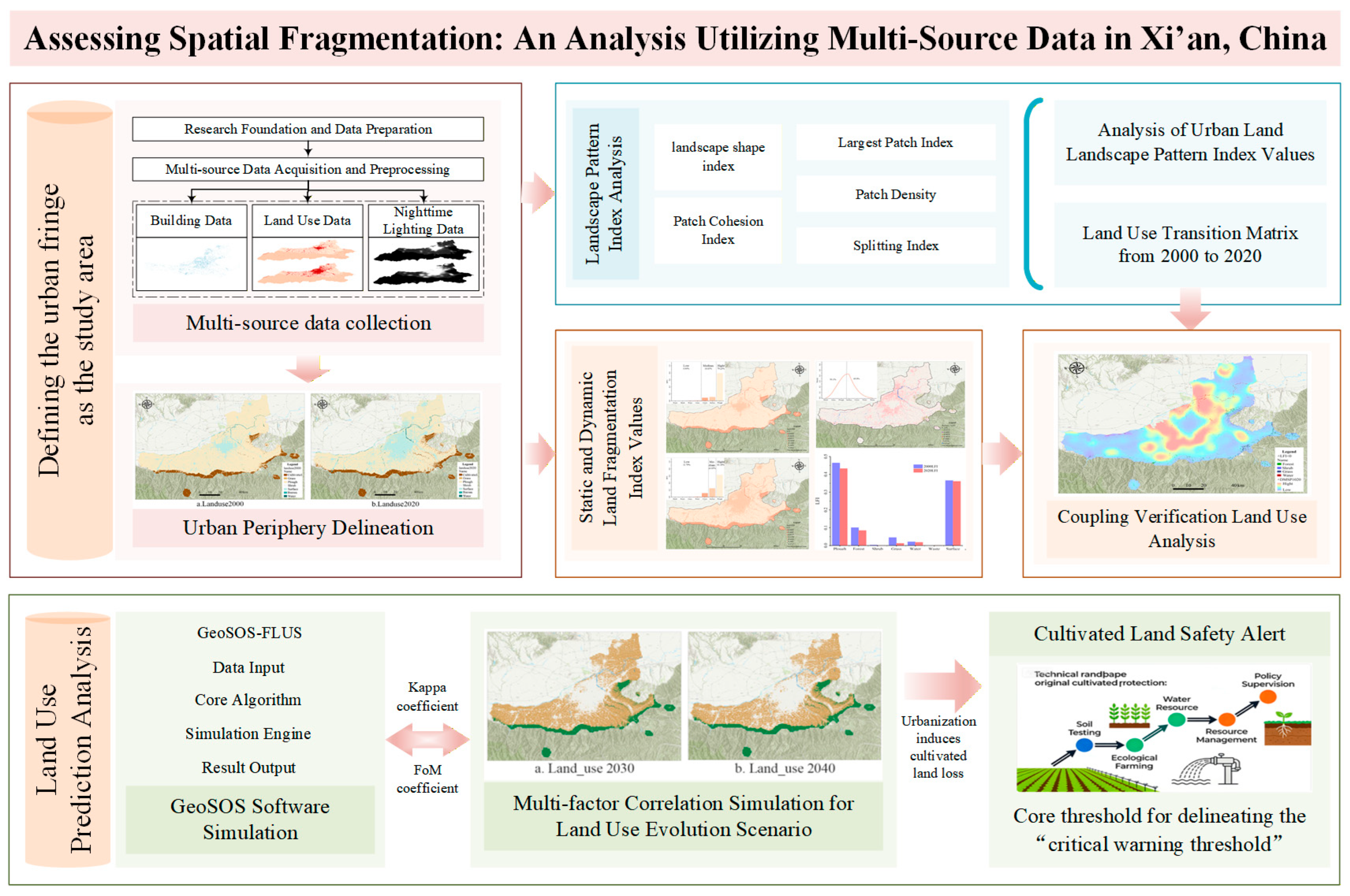
Xi’an serves as an empirical case due to its unique position. It is the only national central city in Northwest China and a Belt and Road hub. These factors make its urbanization both representative and distinctive [50]. This study has four main objectives. First, it delineates the urban fringe using nighttime light data. Second, it examines the evolution of land use structure and spatial patterns, with attention to cropland fragmentation. Third, it couples light data with fragmentation indices to validate spatial correlations. Fourth, it projects land use patterns for 2030 to 2050 and defines thresholds for cropland protection and fragmentation control. This framework addresses the four gaps identified above. First, it integrates multiple data sources and spatial modeling techniques, overcoming the limitations of single-method approaches. Second, it incorporates socio-economic drivers through nighttime light data as a proxy for urbanization intensity. Third, it provides long-term projections (2030–2050) and establishes quantitative warning thresholds, enabling proactive management. Fourth, it focuses specifically on the urban fringe, generating insights tailored to this understudied spatial unit (Figure 1).

This study contributes to the understanding of spatial fragmentation in urban fringe areas through theoretical and methodological advancements. Theoretically, it elucidates the spatial interplay between urban expansion and ecological conservation. This enriches the interdisciplinary nexus of landscape ecology and urban geography. Methodologically, it develops a multi-scale, multi-metric monitoring and assessment framework that offers a replicable methodology for studies in comparable contexts. The findings are expected to inform spatial planning strategies that reconcile urban growth with ecological integrity, thereby enhancing the stability and resilience of urban ecosystems.

2. Data and Methods

2.1. Study Area

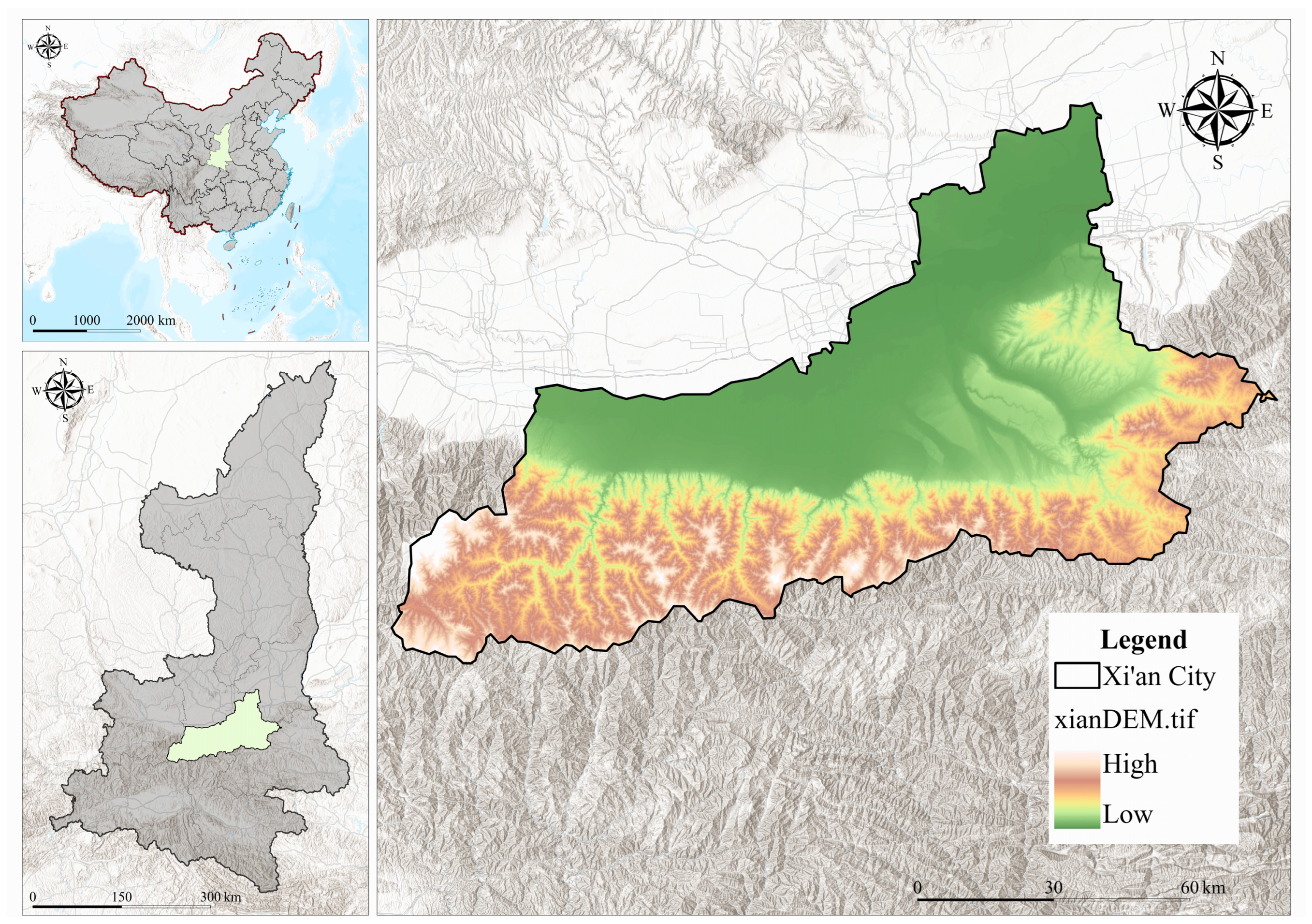
Xi’an is situated in central Shaanxi Province, within the core area of the Guanzhong Plain. It is bordered by the Weihe Plain to the north and the Qinling Mountains to the south. The terrain descends from northwest to southeast, encompassing both plains and mountainous topography [51]. Geographically, Xi’an lies between 107°40′–109°10′ E and 33°42′–34°45′ N. The city experiences a warm temperate semi-humid continental monsoon climate with four distinct seasons. The mean annual temperature ranges from 13 to 14 °C, and annual precipitation averages between 500 and 700 mm [50]. As a major economic hub, Xi’an serves as a key development center in northwestern China and is one of the region’s principal metropolises [52]. In recent years, the city has undergone rapid economic expansion, hosting a population of approximately 12 million, with a population density of about 1200 persons per square kilometer [53]. According to the latest land use survey data, the dominant land use types in Xi’an comprise cultivated land, forest, grassland, construction land, and water bodies (Figure 2).

2.2. Research Data

This study utilizes multiple sources of publicly available data, integrating nighttime light data, land use data, and building data to comprehensively account for relevant influencing factors. The specific datasets are as follows. First, Wu et al. [54] provided DMSP-OLS-like nighttime light data (1992–2024) on the Harvard Dataverse platform. This dataset integrates two types of nighttime light remote sensing observations—DMSP-OLS and SNPP-VIIRS—to reconstruct an improved long-term time-series covering China from 1992 to 2024. Leveraging the high dynamic detection capability of SNPP-VIIRS, the dataset effectively mitigates the pervasive light saturation issue inherent in conventional DMSP-OLS data and enables detailed differentiation of intra-urban spatial structural variations. Second, Zhang et al. [55] provided the global 30 m resolution land cover dynamic dataset (GLC_FCS30D) from the Big Data Center for Sustainable Development Goals. Third, Zhang et al. [56] shared building footprint data on the Zenodo platform. We obtained DEM and slope data from the GEBCO database, and transportation road data from the OpenStreetMap (OSM) road network dataset. These datasets are characterized by high spatial resolution, which enhances the accuracy and reliability of the analysis and ensures the scientific validity and practical relevance of the study’s conclusions (

Table 1. Data sources and features.

Data	Data Source	Functions
Nighttime light data	Harvard database (https://dataverse.harvard.edu/dataset.xhtm (accessed on 20 April 2025))	Primarily used for delineating urban fringe areas and analyzing their spatiotemporal dynamics
Land use data	Big Data Research Center for Sustainable Development (https://data.casearth.cn/thematic/glc_fcs30/314 (accessed on 20 April 2025))	Used to reveal the structural composition and spatial pattern evolution of land use types within the study area
Building data	Zenodo database (https://doi.org/10.5281/zenodo.11397015 (accessed on 20 April 2025))	Provides refined building distribution information to assist in more accurately identifying and delineating the boundaries of urban fringe areas
DEM, Slope	GEBCO (https://www.gebco.net/data-products/ (accessed on 20 April 2025))	Supplies key topographic constraints for subsequent land use change simulations
Transportation road data	OSM (http://www.openstreetmap.org/ (accessed on 20 April 2025))	Serve as critical spatial driving factors to support scenario simulation and prediction of land use patterns

).

The original spatial resolutions of these multi-source datasets exhibited notable differences. The nighttime light imagery had a resolution of 500 m, the land use data had a resolution of 30 m, and the building footprint vector data possessed higher precision. To prevent inconsistencies in spatial resolution and projection datum from affecting the overlay analysis, we conducted the following preprocessing steps. First, we selected the nighttime light data from 2020 for analysis, hereafter referred to as “DMSP2020”. Next, we unified all datasets into the Krasovsky_1940_Albers coordinate system. Using the 30 m resolution as the baseline, we applied a nearest-neighbor resampling algorithm to downscale the 500 m nighttime light imagery. This step ensured that all data maintained consistent spatial positioning and projection coordinate systems, thereby guaranteeing the accuracy of subsequent spatial analyses.

2.3. Research Methods

2.3.1. Nighttime Light Data Processing

In studies utilizing nighttime light data, interference from adjacent areas is a common issue, with the most pronounced effects arising from edge overflow of high-intensity light sources [57]. This light overflow typically occurs in fringe commercial districts, industrial parks, and highway lighting systems. Light diffusion combined with the sensor’s “halo effect” causes illumination to permeate into the edge pixels of the study area, leading to artificially elevated digital number (DN) values. Such inflation of DN values in low-brightness regions can distort analytical outcomes, obscure distinctions between medium- and low-brightness targets, and confound the interpretation of brightness attributes [58].

The light gradient threshold method is based on a key observed characteristic: urban nighttime light intensity exhibits a “gradient decay” pattern as distance from the city center increases [59]. The method quantifies this decay trend and establishes critical thresholds to delineate the urban core, fringe, and rural hinterland, thereby providing an objective basis for defining spatial boundaries in studies of urban spatial structure.

$$G_{i,j}=\mathrm{D}{N}_{i,j}-\mathrm{D}{N}_{i+1,j}$$

(1)

$$G_{i,j}^{\prime }={\displaystyle \frac{D{N}_{i,j}-D{N}_{i+1,j}}{D{N}_{max}-\mathrm{D}{N}_{min}}}$$

(2)

In Formula (1) and (4), $G_{i,j}$ represents the light gradient value of the $i$-th pixel in the $j$-th transect; $D{N}_{i,j}$ denotes the nighttime light intensity of the $i$-th pixel in the $j$-th transect; $D{N}_{i+1,j}$ is the nighttime light intensity of the $(i+1)$-th pixel in the $j$-th transect. In formula (2), $G_{i,j}^{\prime }$ stands for the standardized light gradient value; $D{N}_{max}$, $D{N}_{min}$ are the maximum and minimum values of the nighttime light data in the study area.

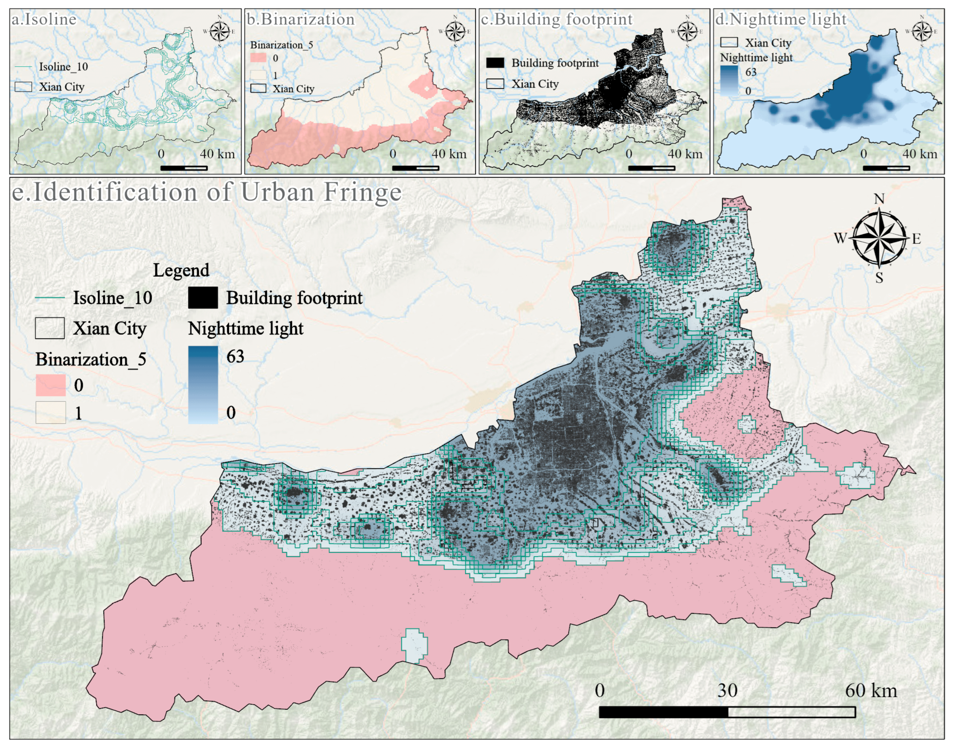
This study employed the light gradient threshold method to delineate the urban rural gradient of Xi’an, identifying the urban fringe based on pixel digital number (DN) values. This approach helps reflect the pattern of urban expansion. We conducted an overlay analysis of several data layers, including contour lines (Figure 3a), nighttime light binarization derived from the gradient threshold method (Figure 3b), building footprint data (Figure 3c), and nighttime light data (Figure 3d). Through this analysis, we delineated the urban fringe, as shown in Figure 3e and summarized in Figure 3.

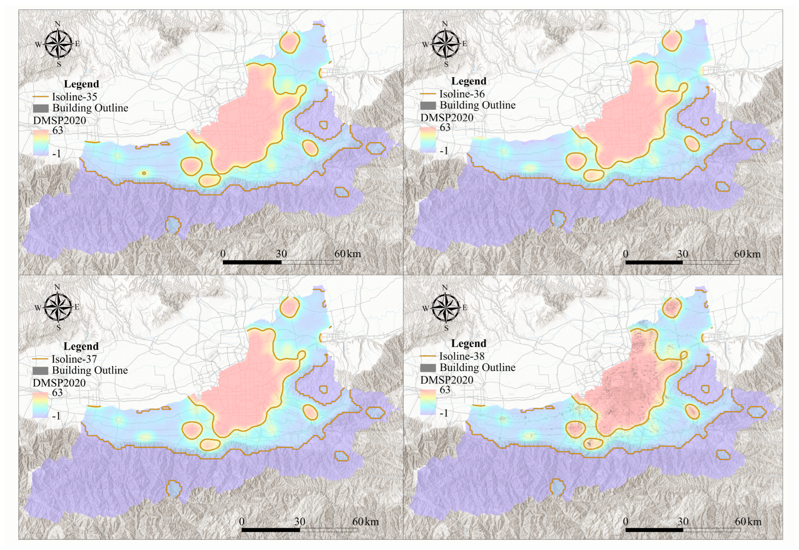
Subsequently, we tested multiple threshold intervals—35, 36, 37, and 38—and validated them against land use and building footprint data (Figure 4) to define the urban core area. The results indicate that the contour line of 35 produced an overly constrained boundary, whereas the lines of 37 and 38 resulted in excessive expansion, incorporating non-urban land such as scattered cropland into the urban area. Among the tested thresholds, the contour line of 36 yielded the most effective delineation of the urban fringe. Its spatial extent closely matched both the built-up area derived from building footprints and the high-value zones of the 2020 nighttime light data. Furthermore, this threshold effectively captured the concentric pattern of clustered urban expansion in Xi’an and aligned well with the natural gradient of decreasing nighttime light intensity from the core to the fringe.

2.3.2. Landscape Pattern Index Analysis

This study integrates gradient analysis with landscape metrics to assess spatial fragmentation within the urban fringe [60]. For this purpose, we selected five metrics: Patch Density (PD), Largest Patch Index (LPI), Landscape Shape Index (LSI), Patch Cohesion Index (COHESION), and Splitting Index (SPLIT). Together, these indices provide a comprehensive, sensitive, and practical framework for characterizing landscape patterns [28,61].

PD quantifies the dispersion of patches. LPI denotes the proportion occupied by the dominant patch type. LSI characterizes shape complexity. COHESION reflects patch connectivity. SPLIT indicates the degree of landscape division. Collectively, these indices capture the core characteristics of fragmentation across multiple dimensions [49,62]. They are effective for representing the current landscape configuration and, through temporal comparison, for revealing evolutionary trends [63]. This approach provides a scientific basis for ecological monitoring and spatial management in the fringe area, thereby effectively supporting the analysis of fragmentation mechanisms and the development of optimization strategies (

Table 2. Descriptions of landscape metrics used in the study [64].

Landscape Metrics	Description
PD	Percentage of landscape by patch type.
LPI	Percentage of landscape occupied by the largest patch of the corresponding type.
LSI	Perimeter to area ratio, indicating overall landscape complexity.
COHESION	Measures patch connectivity and clustering.
SPLIT	Indicates degree of landscape fragmentation.

).

2.3.3. Land Fragmentation Indicators

This study calculates the static Land Fragmentation Index (LFI) for 2000 and 2020 using normalized Edge Density (ED), Patch Density (PD), and normalized Mean Patch Area (MPA), weighted by their average values [36].

$$MP{A}^{\prime }=1-MPA$$

(3)

$$LFI={\displaystyle \frac{1}{3}}ED+{\displaystyle \frac{1}{3}}PD+{\displaystyle \frac{1}{3}}{MPA}^{\prime }$$

(4)

In Formula (3) and (4), $LFI$ is the Land Fragmentation Index, $ED$ is the normalized Edge Density, $PD$ is the normalized Patch Density, and $MPA$ is the normalized Mean Patch Area, while ${MPA}^{\prime }$ is the mean patch area after reverse transformation.

2.3.4. Future Land Use Prediction

This study employs a coupled modeling approach that integrates an Artificial Neural Network (ANN) with Adaptive Inertia Competitive Cellular Automata (CA), combined with Markov Chain analysis [65], multiple driving factors, and an adaptive competition mechanism. The model learns historical relationships between land use and various drivers to simulate the dynamic evolution of land use patterns under natural, socio-economic, and policy constraints. It then projects future land use distribution in Xi’an by forecasting the areal extent of different land types (

Table 3. Driving Factors Used for ANN Model Training.

Driving Factor	Data Source	Resolution	Theoretical Rationale	Standardization Method
DEM	GEBCO	500 m	Topography structures land use patterns by which elevation gradients yield varying development constraints and land utilization types	Min-Max Normalization
Slope	GEBCO	500 m	Slope creates differential land use: conversion favors gentle slopes, stability prevails on steep slopes.	Min-Max Normalization
Highway	OSM	/	Highway fuel agricultural-to-urban conversion by raising accessibility and rent, as location theories predict	Euclidean Distance Standardization
Railway	OSM	/	Railways operate like highways, using improved accessibility to drive urban expansion and intensify land use along their routes	Euclidean Distance Standardization
Road	OSM	/	As key urban rural connectors, major roads shape adjacent land value and guide the distribution of residential and commercial areas through their accessibility	Euclidean Distance Standardization
Water	OSM	/	Water bodies dually shape land use, limiting development in sensitive areas but promoting it in scenic ones, forming a “conservation-development” gradient	Euclidean Distance Standardization

).

$$X_{i,j}^{\prime }={\displaystyle \frac{X_{i,j}-X_{min}}{X_{max}-X_{min}}},$$

(5)

$$P_{k\left(i,j\right)}={\displaystyle \frac{1}{1+e^{-\left({\sum }_{m=1}^{M}wkm\times H_m+b_k\right)}}},$$

(6)

$$T{P}_{k\left(i,j,t\right)}=P_{k\left(i.j\right)}\times N_{k\left(i,j,t\right)}\times C_{k\leftarrow c}\times I_{k\left(t\right)},$$

(7)

$$Kappa={\displaystyle \frac{N{\displaystyle {\sum }_{k=1}^K}{O}_{kk}-{\sum }_{k=1}^K\left(O_{k+}\times O_{+k}\right)}{N^2-{\sum }_{k=1}^K(O_k\times O_{+k})}},$$

(8)

$$FOM={\displaystyle \frac{B}{A+B+C+D}},$$

(9)

In Formula (4), $X_{i,j}^{\prime }$ is the normalized driving factor value of the pixel in row $i$ and column $j$. In Formula (5), $P_{k(i,j)}$ is the suitability probability that the pixel in row $i$ and column $j$ develops into the $k$-th type of land use; $wkm$ is the connection weight between neurons in the hidden layer and the neuron of the $k$-th type of land use in the output layer of the ANN; $H_m$ is the output value of the $m$-th neuron in the hidden layer; $b_k$ is the bias term of the neuron of the $k$-th type of land use in the output layer; and $M$ is the number of neurons in the hidden layer. In Formula (6), $T{P}_{k\left(i,j,t\right)}$ is the total conversion probability that the pixel in row $i$ and column $j$ converts from the current land use type c to the target type $k$ at time $t$; $N_{k\left(i,j,t\right)}$ is the neighborhood influence factor, representing the agglomeration intensity of the $k$-th type of land use around this pixel at time $t$; $C_{k\leftarrow c}$ is the conversion cost, indicating the feasibility of converting from the current type $c$ to the $k$-th type of land use; $I_{k\left(t\right)}$ is the adaptive inertia coefficient. When the area of the $k$-th type of land use does not reach the target at time $t$, $I_{k\left(t\right)}>1$ to increase its conversion priority; otherwise, $I_{k\left(t\right)}<1$ to inhibit conversion. In Formula (7), $N$ is the total number of pixels, $K$ is the number of land use types, $O_{kk}$ is the number of pixels in the confusion matrix where “the true type is k and the simulated type is $k$”, $O_{k+}$ is the total number of pixels of the true $k$-th type of land use, and $O_{+k}$ is the total number of pixels of the simulated $k$-th type of land use. In Formula (8), $A$ is the number of pixels that “actually changed but were predicted to remain unchanged”, $B$ is the number of pixels that “both actually changed and were predicted to change”, $C$ is the number of pixels that “actually changed but were predicted to be other types”, and $D$ is the number of pixels that “actually remained unchanged but were predicted to change”.

3. Results

3.1. Delineation of the Urban Fringe Boundary in Xi’an

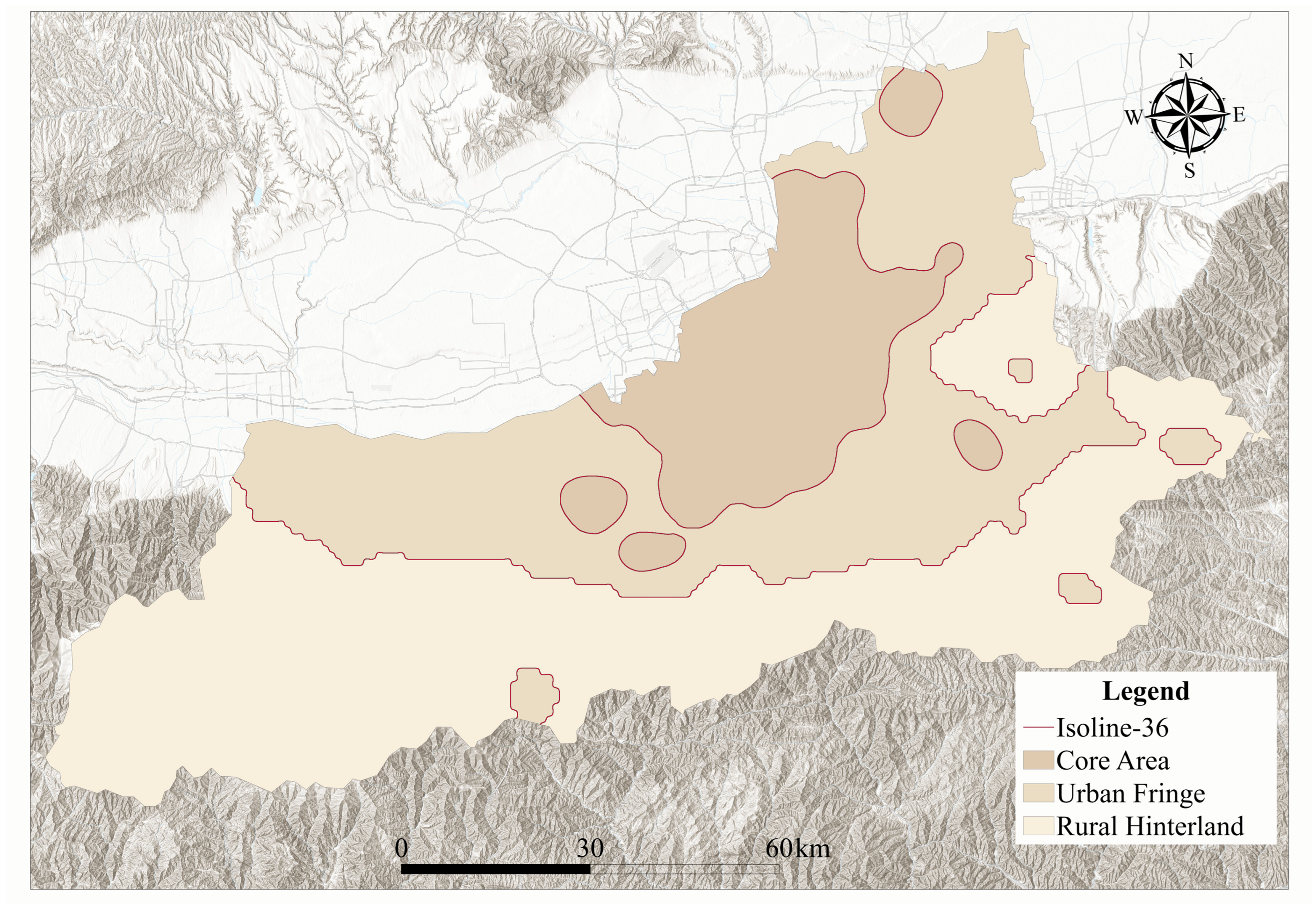
Analysis of nighttime light data reveals a gradual attenuation of light intensity, following a transition sequence of “stable–fluctuating–stable”. Based on this spatial pattern, we developed a schematic diagram delineating a three-zone division: core area, urban fringe, and rural hinterland (Figure 5). We then integrated the data with land use information and quantified the proportional distributions of construction land and cultivated land across these three zones.

Table 4. Proportions in Different Regions in 2020.

	Built Up Share	Cultivated Land Share
Core Area	71.69%	22.05%
Urban Fringe	27.26%	68.65%
Rural Hinterland	1.05%	9.30%

summarizes the results. In the core area, construction land accounts for 71.69%, while cultivated land comprises 22.05%. In the urban fringe, the proportion of construction land decreases to 27.26%, with cultivated land representing 68.65%. In the rural hinterland, construction land constitutes only 1.05%, and cultivated land accounts for 9.30%.

The lower proportion of cultivated land in the rural hinterland compared to the urban core area primarily results from the distinctive spatial configuration of the study area. The “rural hinterland” in this study encompasses the mountainous region on the northern slope of the Qinling Mountains, an area characterized by significant topographic relief. Forest land dominates as the primary land use type, with cultivated land appearing only sparsely in river valleys, which explains its very low proportion. In contrast, the urban core area lies in the Weihe Plain, where flat terrain allows a considerable amount of high-quality farmland to remain, resulting in a higher proportion of cultivated land. This finding reflects the coupling characteristics of urban-rural spatial patterns and topographic conditions in Xi’an and is consistent with the actual regional situation.

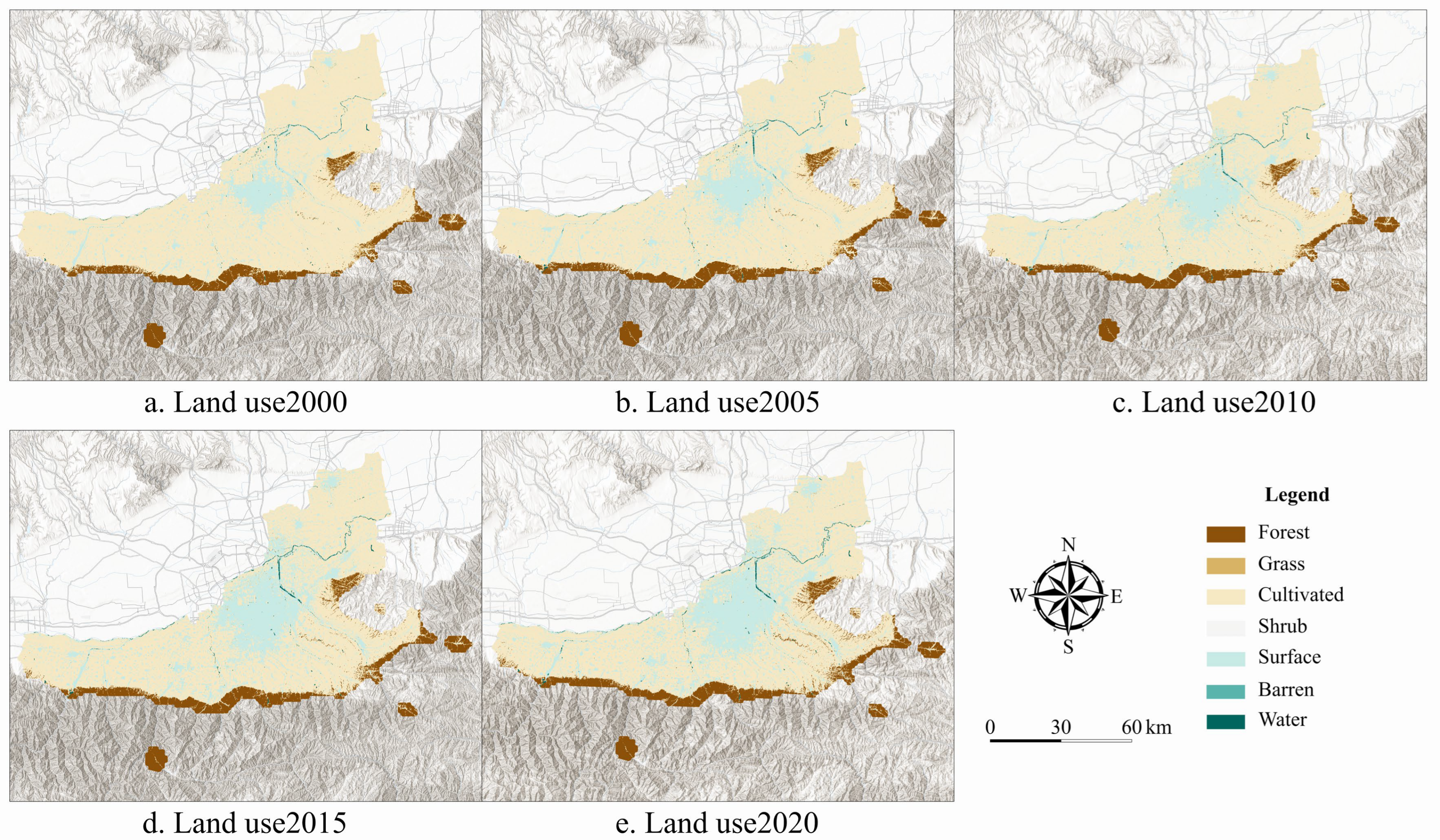
We delineated the spatial structure into three zones: core area, urban fringe, and rural hinterland. Based on this delineation, we identified the urban fringe. Subsequent analysis will focus on two primary study areas—the core area and the delineated fringe—as illustrated in Figure 6.

3.2. Analysis of Urban Land Landscape Pattern Index Values

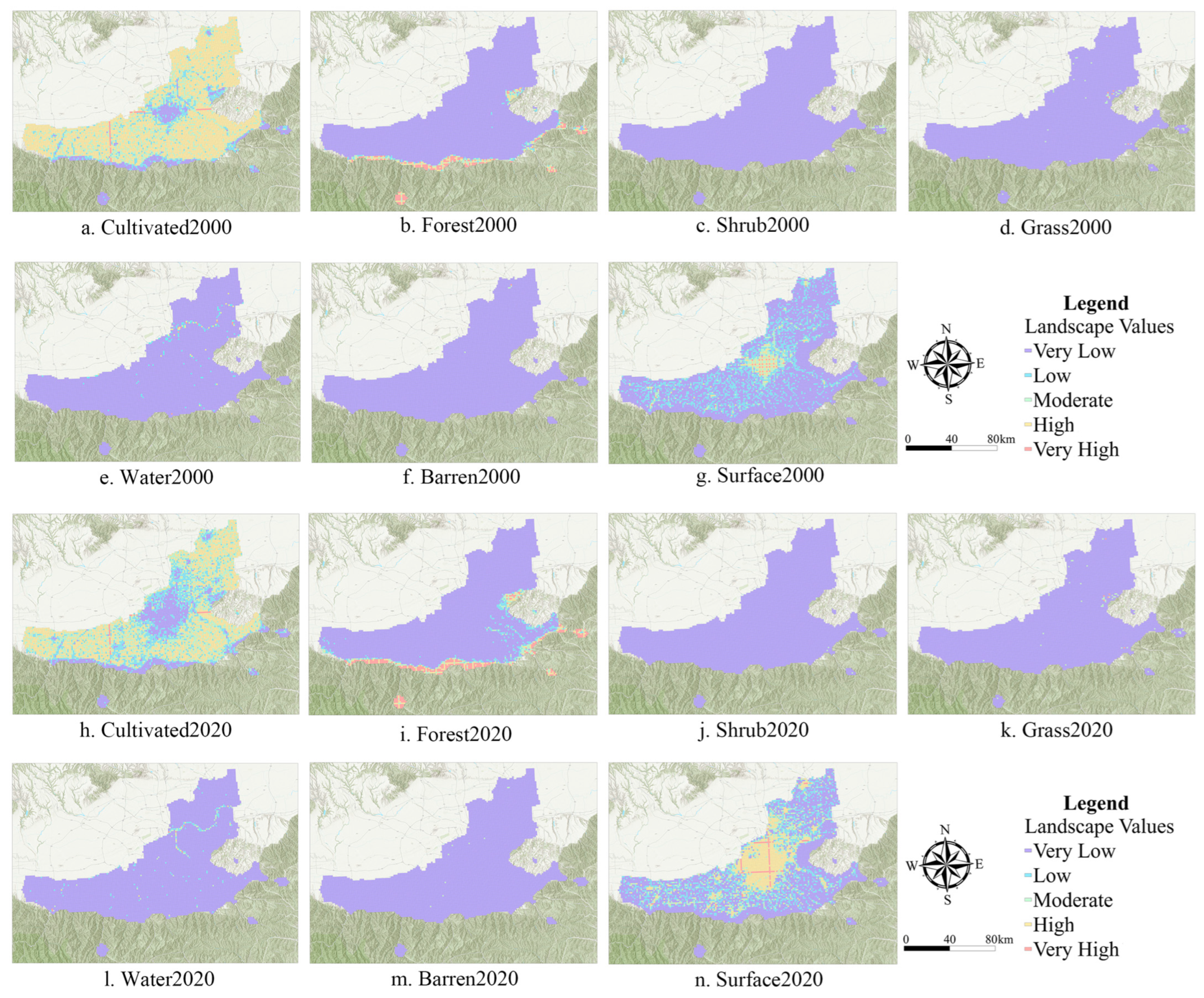
We analyzed Xi’an’s land use data from 2000 to 2020 using Fragstats4.2 software. The results showed that five key metrics changed across land use types in the urban fringe, revealing distinctive gradients in rate, intensity, and heterogeneity.

Table 5. Comparative Analysis of Change Indices of Each Land Use Type in Xi’an in 2000 and 2020.

TYPE	ΔPD	ΔLPI	ΔLSI	ΔCOHESION	ΔSPLIT
Cultivated	0.2241	−17.4479	30.6971	−0.0300	1.1137
Forest	0.0906	2.7410	5.2518	0.2109	−6.23 × 102
Shrub	−0.0152	−0.0008	−6.8917	−13.2192	5.65 × 109
Grass	−0.0738	−0.0121	−12.9652	−23.4130	6.65 × 107
Water	−0.0070	0.0369	−22.0466	−41.2865	3.41 × 109
Barren	0.0054	0.0001	26.1716	47.0765	−1.12 × 1010
Surface	−0.0069	8.8432	7.1816	2.1064	−5.04 × 102

and Figure 7 summarize these findings.

Fragmentation characteristics varied significantly among land use categories. Cultivated land underwent considerable areal loss, exhibiting high fragmentation and declining connectivity. Forest cover expanded with low fragmentation and slightly improved connectivity. Shrubland showed moderate area loss, accompanied by high fragmentation and markedly reduced connectivity. Grassland area decreased, experiencing both increased fragmentation and diminished connectivity. Water bodies showed a slight reduction in area, with heightened fragmentation and reduced connectivity. Barren land expanded slightly, retaining high fragmentation but showing significantly enhanced connectivity. Impervious surfaces expanded markedly, exhibiting low fragmentation and moderately improved connectivity.

Notably, four land use types—cultivated land, shrubland, grassland, and water bodies—displayed accelerated or sustained high fragmentation intensity, along with significantly increased spatial heterogeneity. This pattern indicates that these ecosystems experienced substantial disturbances. In contrast, forests and impervious surfaces demonstrated distinct consolidation trends, characterized by low-speed integration and reduced spatial heterogeneity. Forests reinforced their ecological functions, while impervious surfaces concentrated urban development.

Barren land underwent a notable transition from extreme dispersion toward patch integration. This reversal was reflected in substantial improvements across multiple fragmentation-related metrics, representing a distinct trajectory of landscape reorganization within the urban fringe.

We conducted a cross-tabulation analysis of land use transitions between the two study periods by overlaying classified land use data and quantifying the conversion areas.

Table 6. Land Use Transition Matrix from 2000 to 2020(%).

	2020	Cultivated	Forest	Shrub	Grass	Water	Barren	Surface
2000
Cultivated		78.09	2.53	0.002	0.11	0.40	0.01	18.86
Forest		3.13	96.28	0.03	0.39	0.08	\	0.08
Shrub		4.84	89.42	1.35	4.38	\	\	\
Grass		26.62	58.39	0.29	10.14	1.29	0.13	3.14
Water		37.72	0.66	\	0.27	35.10	\	26.25
Barren		14.94	\	\	4.19	\	5.26	75.61
Surface		8.52	0.2	\	0.02	1.95	0.001	89.49

Note: “\” denotes a zero value.

summarizes the results, which reveal distinct transition patterns. Cultivated land underwent extensive conversion, primarily turning into impervious surfaces. Forest area exhibited net growth, mainly from cultivated land and grassland. Both shrubland and grassland showed net decreases, with substantial portions converting to forest. Water bodies experienced a net areal increase, derived partly from cultivated land and partly from impervious surfaces. Impervious surfaces expanded significantly, with much of the existing area retained and large-scale conversion occurring from cultivated land.

3.3. Differences in Static and Dynamic Land Fragmentation Index Values

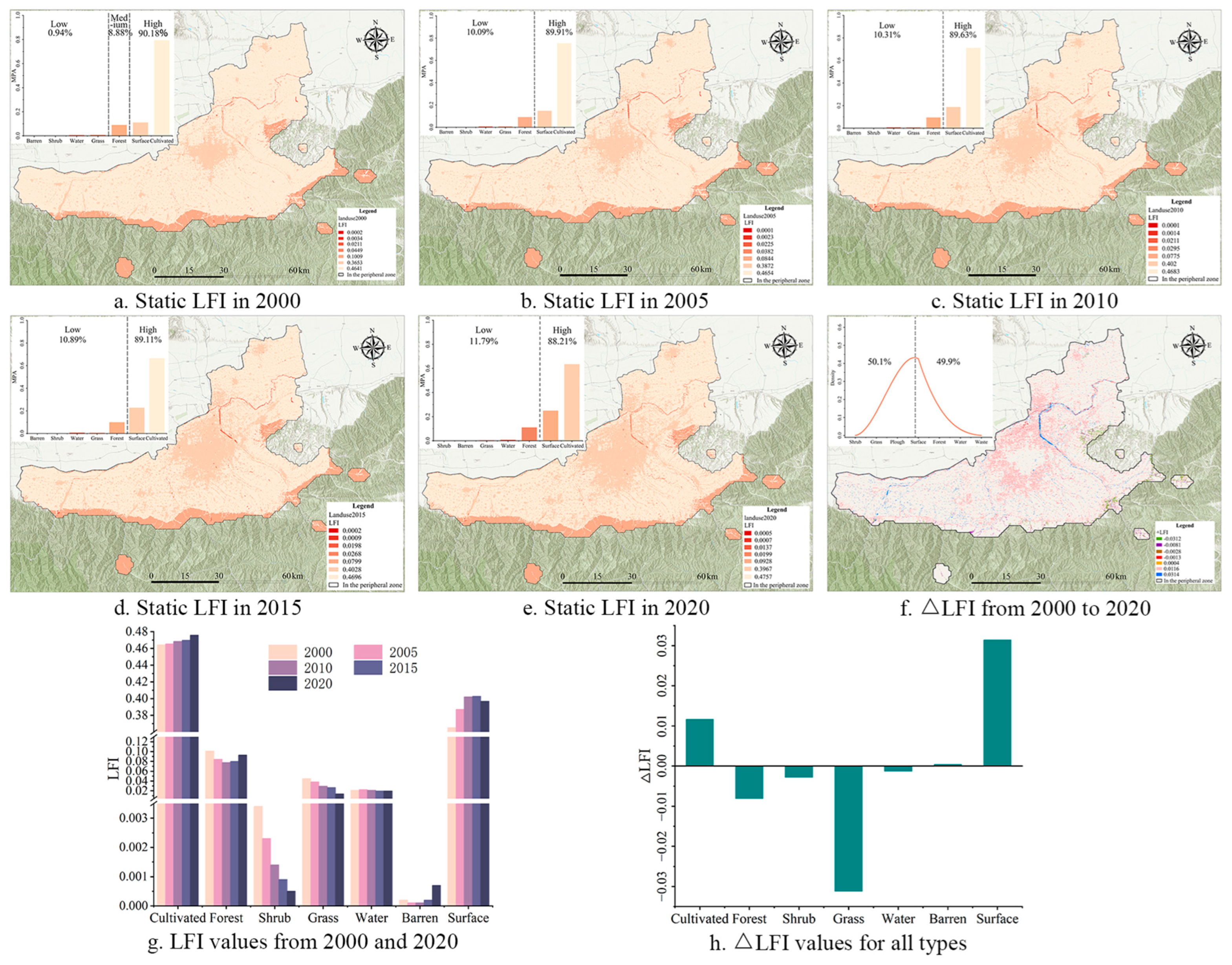
Based on the calculated LFI values, we classify areas with LFI < 0.1 as having low static land fragmentation, and those with LFI > 0.3 as having high static land fragmentation. Between 2000 and 2020, the proportion of landscapes at different fragmentation levels exhibited a generally gradual trend without significant fluctuations, remaining relatively stable overall.

In 2000, several landscape types had an LFI below 0.1, including barren land, shrubland, and water bodies, while cultivated land and impervious surfaces exceeded 0.3. Forest landscapes fell within the intermediate range of 0.1–0.3 (Figure 8a). From 2005 to 2020, this pattern persisted: barren land, shrubland, water bodies, and forest all maintained an LFI below 0.1, whereas cultivated land and impervious surfaces consistently showed values above 0.3 (Figure 8b–e). During this period, the share of landscapes with low static fragmentation—including barren land, shrubland, water bodies, and forest—increased from 10.09% to 11.79%. In contrast, the proportion of cultivated land and impervious surfaces, which exhibited comparatively higher static fragmentation, decreased from 88.91% to 88.21%.

The distribution of the dynamic Land Fragmentation Index (ΔLFI) differed markedly from the static pattern. Specifically, 50.1% of the landscape experienced a reduction in fragmentation (ΔLFI < 0), most evident in forest and grassland. Conversely, impervious surfaces showed an increase in fragmentation (ΔLFI > 0). Fragmentation levels in shrubland, water bodies, and barren land remained relatively stable, showing no significant changes (ΔLFI≈0) (Figure 8f).

The analysis of Xi’an revealed distinct patterns in static fragmentation. Cultivated land recorded the highest levels, while water bodies and barren land recorded the lowest. Furthermore, cultivated land and impervious surfaces registered higher static LFI values than other land use types in both 2000 and 2020. The integration of dynamic fragmentation indicators reveals a more nuanced story: although cultivated land maintained a relatively stable and high level of static fragmentation throughout the period, it simultaneously experienced an intensification of the fragmentation process (Figure 8g,h).

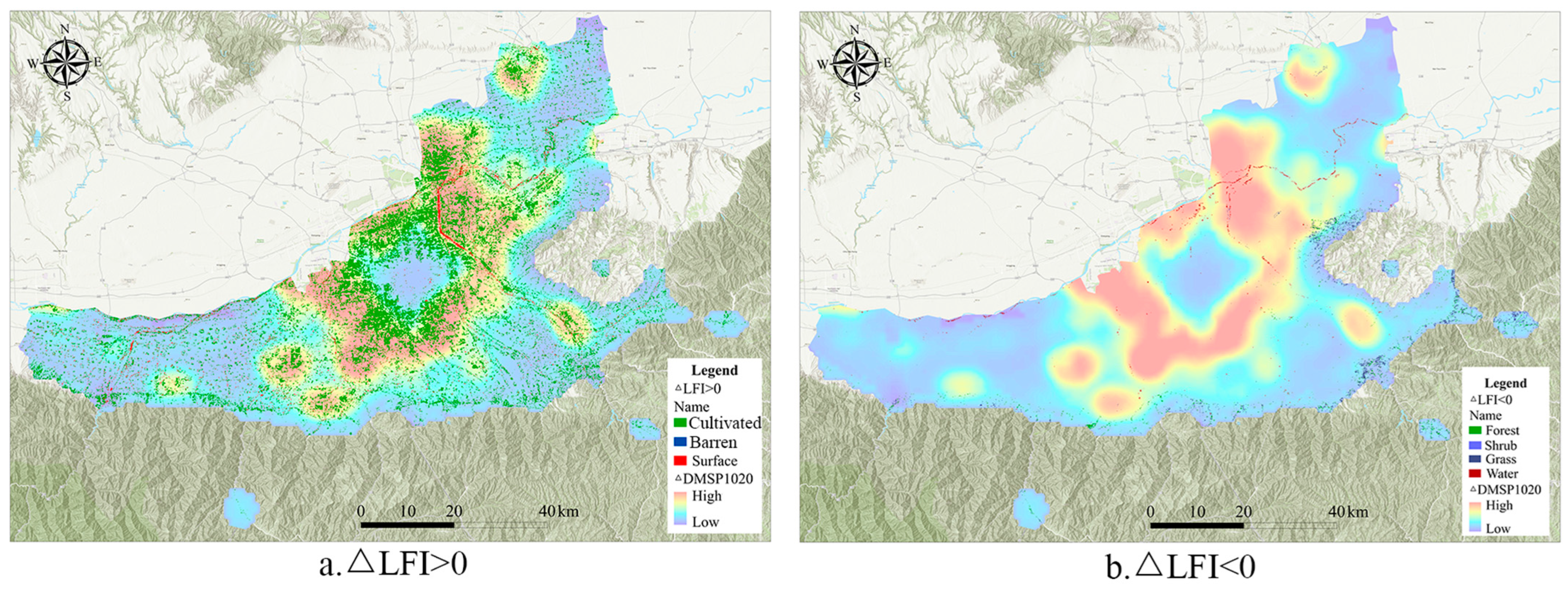
The static LFI characterizes the inherent fragmentation state, while the dynamic LFI (ΔLFI) tracks its changes over time. Their combined use enables a holistic understanding of fragmentation dynamics. This study leverages nighttime light data as an indicator of urban expansion and uses ΔLFI as a metric of fragmentation change to examine their spatial coupling. The analytical procedure involved extracting areas with positive and negative ΔLFI values—where positive values signify intensified fragmentation and negative values indicate reduced fragmentation—and spatially comparing them with urban expansion patterns derived from nighttime light data.

We then examined the coupling relationship between urbanization and fragmentation (Figure 9). An ordinary least squares (OLS) regression was first conducted. The results showed significant correlations between light increase and positive fragmentation, as well as between light decrease and negative fragmentation. However, the model fit was low (R² = 0.03, p < 0.01). We then tested the spatial autocorrelation of the OLS residuals and detected significant positive spatial autocorrelation (Moran’s I = 0.985, p < 0.001), indicating that OLS cannot account for spatial dependence.

To address this issue, we applied a geographically weighted regression (GWR) for correction. The GWR effectively removed residual spatial clustering and significantly improved the model fit (R² = 0.65, p < 0.01). The results show that areas with large increases in nighttime light experience intense human activity and exhibit significantly higher fragmentation. In contrast, areas with low light intensity maintain stable land use and lower fragmentation. The overall spatial pattern is highly consistent, confirming that urbanization coincides with fragmentation in expansion zones, while low-intensity areas retain relatively intact and stable landscape patterns.

3.4. Land Use Prediction Analysis

To enhance the reproducibility and transparency of this study, we recorded the key parameter settings and constraint conditions used in the land use change simulation, including simulation control parameters (

Table 7. Simulation setting parameters.

Simulation Setting	Number
Maximum Number of Iteration	300
Neighborhood (odd)	3
Accelerate (0–1)	0.1
Thread	8

), a land use transition cost matrix (

Table 8. Cost Matrix analysis.

Cost Matrix	Plough	Forest	Shrub	Grass	Water	Waste	Surface
Plough	1	1	1	1	1	1	1
Forest	1	1	1	1	1	0	1
Shrub	1	1	1	1	0	0	0
Grass	1	1	1	1	1	1	1
Water	1	1	0	1	1	0	1
Waste	1	0	0	1	0	1	1
Surface	1	1	0	1	1	1	1

), and neighborhood weight coefficients (

Table 9. Weight of Neighborhood analysis.

	Plough	Forest	Shrub	Grass	Water	Waste	Surface
Weight of Neighborhood	0.7	0.4	0.5	0.5	0.4	0.4	1

). We calibrated the model using land use data for Xi’an at five-year intervals from 2000 to 2020. Comparison of the simulation results with actual land use patterns indicated satisfactory overall model performance, with a Kappa coefficient of 0.823 and a FoM index of 0.750. These findings suggest that the model can effectively capture the general trends of land use evolution under future urbanization in Xi’an.

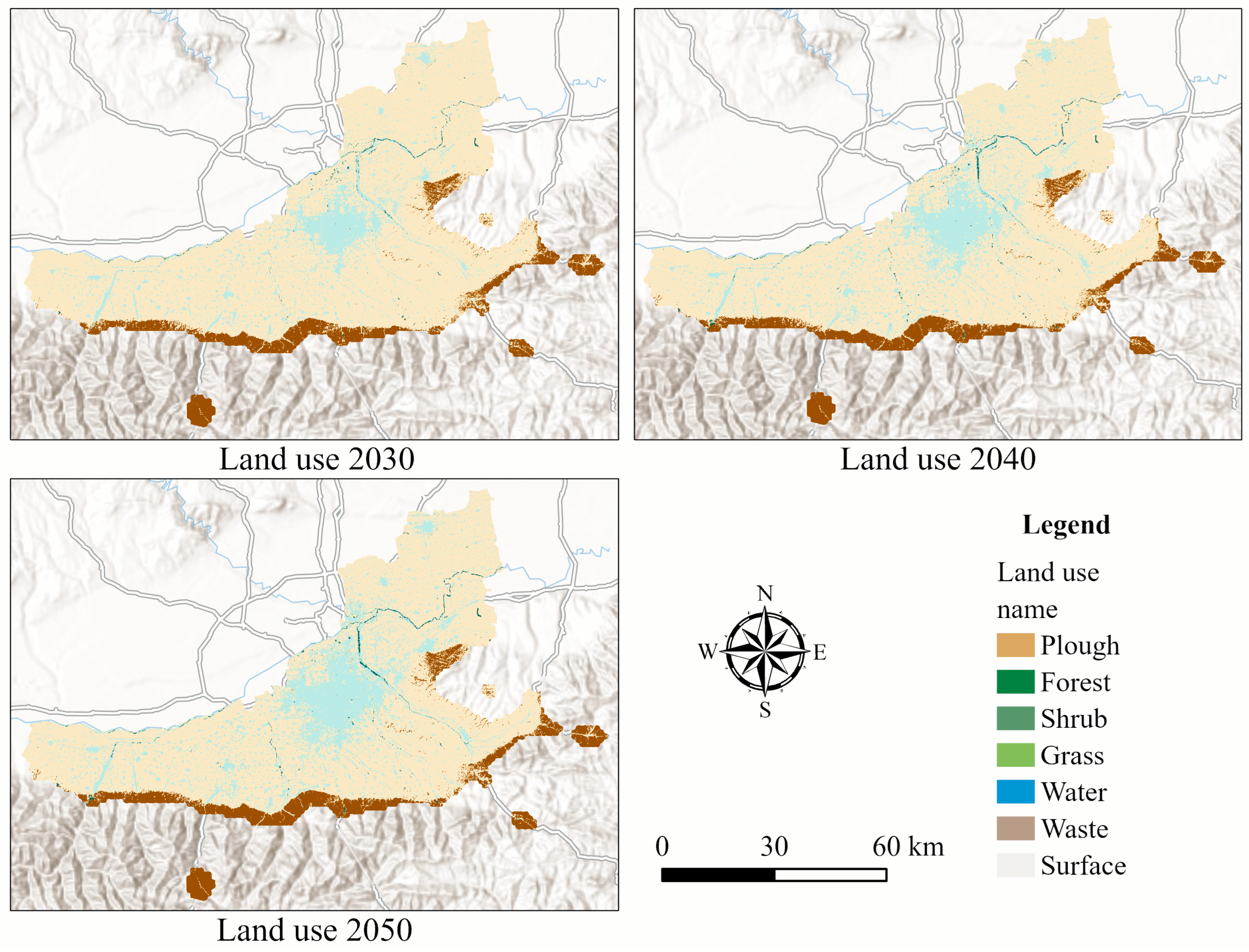
Based on this, we projected three land use scenarios for the years 2030, 2040, and 2050 (Figure 10). These projections provide data support for the subsequent dynamic analysis of cropland fragmentation. A temporal analysis from 2020 to 2050 reveals an important trend: the growth of urban impervious surfaces is closely associated with the ongoing development of the Xixian New Area. This district serves as a key growth pole for Xi’an and plays a central role in strategies for industrial clustering and urban functional expansion. Extensive construction activities within the district act as the primary driver of impervious surface spread. This process has led to the progressive conversion of land—particularly in the central and urban fringe parts of the new district—from agriculture or natural ecosystems to urban construction land. The development of substantial impervious infrastructure, including roads, buildings, and plazas, is driving this change. Consequently, the region is undergoing a significant transformation in its land cover patterns.

Rapid urbanization leads to the uncontrolled spread of construction land and the continuous expansion of impervious surfaces. These processes encroach on high-quality cultivated land, causing a sharp decline in its area while fragmenting its patches and reducing spatial connectivity. Collectively, these changes threaten regional food security and ecosystem stability.

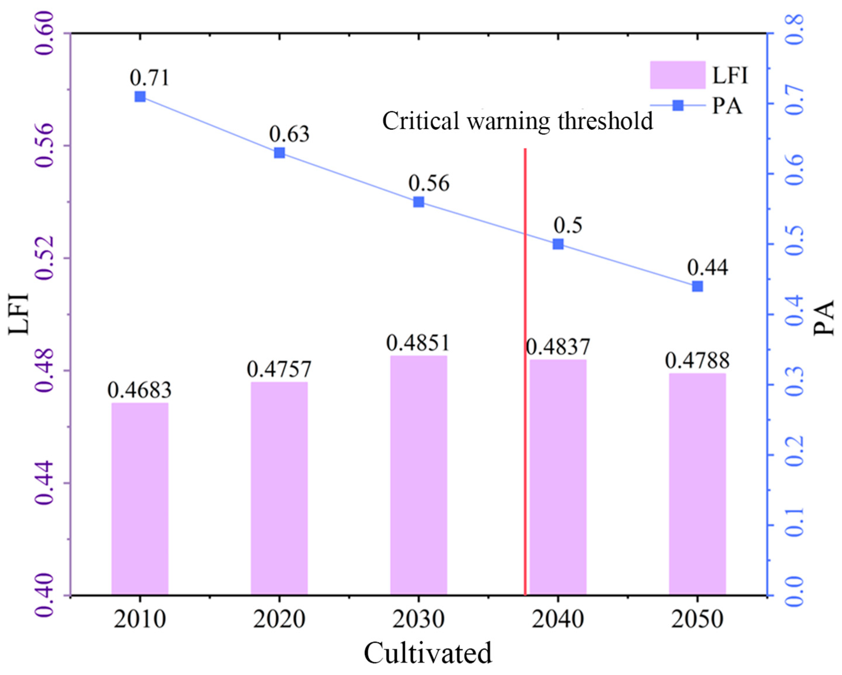
According to the Technical Regulations for Cultivated Land Safety Early Warning (TD/T 1080–2023), a cumulative decline of 20% or more in cultivated land triggers a red-level warning. The Land Use Master Plan of Xi’an (1997–2010) is an early programmatic document for land use control. Therefore, this study selected 2010 as the baseline year, when the cultivated land fragmentation index was 0.4683 and the proportion of cultivated land was 0.71. Based on this baseline, the study analyzed the evolution of cultivated land fragmentation in Xi’an from 2010 to 2050.

The results show a phased pattern. As urban expansion continued, the share of cultivated land declined gradually, while the fragmentation index first increased and then decreased slightly. From 2010 to 2030, the cultivated land proportion fell from 0.71 to 0.56, and the fragmentation index rose from 0.4683 to 0.4851. This finding suggests that cultivated land patches became increasingly separated and fragmented, with fragmentation intensifying significantly.

Around 2040, the cultivated land proportion dropped to approximately 0.51, and the fragmentation index reached a temporary peak. The average patch area continued to shrink, urban fringe complexity increased, and spatial connectivity fell to a low point. This marks a critical early warning node at which the ecological functions of cultivated land face significant risk. Although the fragmentation index then showed a slight decline, it remained relatively high, indicating that the stability and service functions of the cultivated land ecosystem have been irreversibly affected.

This trend reveals a coupled relationship between cultivated land reduction and fragmentation intensification. These findings provide an important early warning reference for cultivated land protection and fragmentation control in Xi’an (Figure 11).

4. Discussion

4.1. Spatial Fragmentation Characteristics and Driving Mechanisms of the Urban Fringe in Xi’an

The urban fringe of Xi’an serves as a critical transitional space between urban and rural areas. Between 2000 and 2020, this region exhibited significant spatial fragmentation. It also showed a pronounced differentiation of land use types. These patterns emerged from two concurrent processes: urban expansion and ecological policy regulation [66]. The boundary of this fringe, as delineated in this study, closely corresponds with the actual land use structure. Internally, the land use composition includes 27.26% built-up land and 68.65% cultivated land (Table 4, Figure 5). This mixed structure contrasts clearly with the urban core, which features built-up land dominance and high-density development, as well as with the rural hinterland, which follows a low-intensity development pattern. Consequently, this area constitutes a highly fragmented zone of urban-rural interaction [12], providing a scientifically defined spatial framework for subsequent analyses.

An examination of core fragmentation characteristics reveals that cultivated land experienced the most significant fragmentation among all land types. From 2000 to 2020, its PD increased by 0.2241, while its LPI decreased substantially by 17.4479 (Table 5, Figure 7). This metric profile reflects a pattern of “high-speed fragmentation and concentrated contraction”. Analysis of the land use transition matrix confirms that this pattern resulted from the extensive conversion of cultivated land to impervious surfaces, a process closely associated with Xi’an’s rapid urbanization. During this period, the urbanization rate increased from 42.0% to 73.4%, and built-up areas expanded by 243% [53].

In contrast, forest cover demonstrated a pattern of “slow expansion and contiguous strengthening”, facilitated by the Grain-for-Green Program and ecological protections in the Qinling Mountains. Simultaneously, impervious surfaces (dominated by construction land) expanded via a “gap-filling” approach, achieving contiguous aggregation. Evidence includes a marginal decrease in PD (–0.0069) and a marked increase in LPI (8.8432). This pattern is consistent with the “concentrated development” approach mandated by the Xi’an Land Space Master Plan and indicates a pronounced urban spatial agglomeration effect [67].

A key finding is the emergence of “latent fragmentation”. The areal extent of shrubland, grassland, and water bodies remained largely stable, yet their landscape connectivity declined markedly, with the COHESION index showing declines of 13.2192, 23.4130, and 41.2865, respectively (Table 5). We hypothesize that this pattern results from the “point-based development” model prevalent in the urban fringe. In this model, dispersed developments—such as rural tourism facilities and small industrial parks—consume minimal ecological land in terms of area but significantly fragment the connectivity of ecological patches, creating a latent risk characterized by functional impairment without substantial area reduction.

Moreover, we found a significant spatial correlation (R² = 0.65, p < 0.01) between sharp increases in nighttime light emissions and areas of heightened fragmentation (ΔLFI > 0). This provides further evidence that urban expansion is a central driver of this process. Major development hubs, including the Xixian New Area and Lintong, exhibit a colocation of intensified nighttime lights and increased fragmentation, supporting the value of nighttime light data as an efficient tool for identifying regions at risk of fragmentation (Figure 9).

4.2. Land Use Prediction and Planning Early Warning Value for the Urban Fringe of Xi’an

The land use projection generated by the GeoSOS-FLUS2.4 software’s ANN-CA-Markov model demonstrates high reliability (Kappa = 0.823, FoM = 0.75) (Figure 10) [65], revealing key evolutionary trends and early warning points for the urban fringe of Xi’an from 2030 to 2050. The projection suggests that impervious surfaces will continue to expand, showing a strong correlation with the ongoing development of the Xixian New Area. Consequently, cultivated land and grassland in and around the new district will gradually convert to construction land. This land use change reflects an inevitable requirement for Xi’an as a core city in Northwest China to expand its development space and accommodate new industrial functions. However, this trajectory also presents potential risks, including ecological degradation and challenges to food security [8].

A key early warning point concerns cultivated land protection. Using 2010 as the baseline year—when the cultivated land proportion was 0.71 and its Land Fragmentation Index (LFI) was 0.4683—projections indicate that impervious surface expansion will reduce the cultivated land proportion to approximately 0.51. This represents a 20% decrease from the baseline, reaching the predefined “critical warning threshold”. Concurrently, the LFI for cultivated land will rise to 0.4839, indicating increased patch fragmentation and a consequent decline in large-scale agricultural productivity. These changes will pose considerable challenges to both food security and the stability of agricultural ecosystems [2]. The identified threshold addresses a gap in existing studies, which often describe spatial fragmentation patterns without establishing quantitative warning thresholds [28,30,68,69]. Our finding provides a critical temporal reference for setting phased cultivated land protection targets in Xi’an.

The urban fringe is a transitional zone where urban and rural land uses intersect and land change occurs most intensely. It is also a key area where urbanization drives cultivated land fragmentation. Unchecked urban expansion continues to split ecological land and weaken urban ecological security patterns [12]. Existing fragmentation research has largely focused on methods, drivers, impacts, and regional cases. Studies employ remote sensing, landscape metrics, and spatial regression, yet most rely on single-method approaches and rarely integrate multiple techniques [27]. Driver analyses emphasize physical factors like terrain and roads, while overlooking socioeconomic influences such as policy and economic change [28]. Ecological assessments often use landscape indicators to infer risks, but lack long-term predictions for proactive management [42]. Regionally, European and North American studies reveal contrasting patterns. In southern Europe, fragmentation arises from low-density housing and transport networks, with a focus on post-hoc restoration. North American research uses high-resolution imagery and habitat models but rarely incorporates nighttime light data to capture human activity intensity [30]. Fragmentation here is market-driven, with relatively small cultivated land losses, and existing studies lack early-warning thresholds [44]. Unlike these mature regions, central-western Chinese cities like Xi’an experience rapid outward expansion that continuously consumes cultivated land and creates sprawling spatial patterns. To address research gaps, our study integrates nighttime light thresholding for boundary detection, GWR for spatial variation analysis, and FLUS for scenario simulation. We also set 0.51 as the early-warning threshold for cultivated land proportion, aligning with national farmland protection policies [31]. Overall, current research suffers from weak method integration, insufficient attention to socioeconomic drivers, and a lack of urban fringe focus. China’s rapidly urbanizing regions need proactive warnings, unlike developed countries that emphasize post-hoc restoration. Using Xi’an as a case, our study helps fill these gaps and offers practical insights for fringe governance in developing cities [47].

4.3. Implications and Limitations

The main contribution of this study lies in the development of an integrated analytical framework for spatial fragmentation in the urban fringe. Methodologically, it delineates the dynamic fringe area using the light gradient threshold method and couples nighttime light data with the dynamic land fragmentation index (ΔLFI), providing empirical evidence that “urban expansion dominates fragmentation” (R² = 0.65, p < 0.01). Theoretically, by combining static and dynamic indices, it reveals a “latent fragmentation” phenomenon in ecological land, characterized by “area stability but declining connectivity”. In practice, through ANN-CA-Markov model projections, it proposes a quantitative threshold for a “critical warning threshold”, offering a clear early-warning node for cultivated land protection and spatial regulation.

This study has several limitations. First, the equal-weight construction of the Land Fragmentation Index (LFI) oversimplifies the heterogeneous responses of different landscapes to its indicators [36]. Second, landscape metric approaches cannot accurately quantify the impacts of fragmentation on specific ecosystem services, such as biodiversity. Third, the limited temporal resolution of input datasets and classification uncertainties in land-use products may introduce bias into fragmentation assessments. Fourth, the driver analysis does not capture the spatially heterogeneous contributions of sub-factors. Future research should integrate ecosystem service models with spatial regression methods to quantify ecological losses and identify differentiated driving mechanisms. It should also incorporate overseas case comparisons to enrich research insights.

5. Conclusions

This study investigates the urban fringe of Xi’an by integrating multi-source data, including nighttime light imagery, land use maps, and building footprints. We delineated the fringe boundary using a light gradient threshold method and employed landscape metrics and spatial coupling analysis to assess spatial fragmentation characteristics from 2000 to 2020. Future land use trends for 2030–2050 were then projected using the ANN-CA-Markov model in GeoSOS software. The results reveal distinct land use dynamics in the fringe area between 2000 and 2020. Cultivated land underwent rapid fragmentation and shrinkage, with significant conversion to impervious surfaces. Forest cover expanded slowly and showed improved patch connectivity, while impervious surfaces exhibited aggregation through infill development. Ecological lands such as shrubland experienced increased fragmentation. Urban expansion was the primary driver of these changes, and nighttime light data proved effective for monitoring fragmentation processes. Projections indicate that the proportion of cultivated land will decline from 0.71 in 2010 to 0.51, while its Land Fragmentation Index (LFI) will rise to 0.4839, reaching the predefined “critical warning threshold”.

The analytical framework follows a clear logic—driving factors → spatiotemporal evolution → ecological effects—and helps identify key issues and early-warning indicators of spatial fragmentation in Xi’an’s urban fringe. Our findings offer a scientific basis for land spatial planning, cultivated land protection, and ecological restoration in the city. Furthermore, they provide valuable references for other rapidly urbanizing cities in western China that seek to balance urban expansion with ecological conservation in pursuit of sustainable development.

References

1. UN-Habitat. Envisaging the Future of Cities; UN-Habitat: Nairobi, Kenya, 2022. [Google Scholar]
2. Cox, D.T.; Shanahan, D.F.; Hudson, H.L.; Fuller, R.A.; Gaston, K.J. The impact of urbanisation on nature dose and the implications for human health. Landsc. Urban Plan. 2018, 179, 72–80. [Google Scholar] [CrossRef]
3. Xiong, J.; Yang, Y.; Yang, L.; Yang, D. Asymmetric shifts in precipitation due to urbanization across global cities. Nat. Commun. 2025, 16, 5802. [Google Scholar] [CrossRef] [PubMed]
4. Wu, K.; Xing, A.; Wei, G.; Xin, H.; Wei, Y.; Su, L.; Zhou, J. Evaluation of coupling coordination degree between tourism urbanization and ecosystem services in urban agglomerations in the yellow river basin. Sci. Rep. 2025, 15, 22427. [Google Scholar] [CrossRef] [PubMed]
5. Turner, B.L., II; Kasperson, R.E.; Matson, P.A.; McCarthy, J.J.; Corell, R.W.; Christensen, L.; Eckley, N.; Kasperson, J.X.; Luers, A.; Martello, M.L.; et al. A Framework for Vulnerability Analysis in Sustainability Science. Proc. Natl. Acad. Sci. USA 2003, 100, 8074–8079. [Google Scholar] [CrossRef] [PubMed]
6. Cyril, S.; Oldroyd, J.C.; Renzaho, A. Urbanisation, urbanicity, and health: A systematic review of the reliability and validity of urbanicity scales. BMC Public Health 2013, 13, 513. [Google Scholar] [CrossRef] [PubMed]
7. Inostroza, L.; Baur, R.; Csaplovics, E. Urban sprawl and fragmentation in Latin America: A dynamic quantification and characterization of spatial patterns. J. Environ. Manag. 2013, 115, 87–97. [Google Scholar] [CrossRef] [PubMed]
8. Dijkstra, L.; Florczyk, A.J.; Freire, S.; Kemper, T.; Melchiorri, M.; Pesaresi, M.; Schiavina, M. Applying the Degree of Urbanisation to the globe: A new harmonised definition reveals a different picture of global urbanisation. J. Urban Econ. 2021, 125, 103312. [Google Scholar] [CrossRef]
9. Antrop, M. Landscape change and the urbanization process in Europe. Landsc. Urban Plan. 2004, 67, 9–26. [Google Scholar] [CrossRef]
10. Fu, Y.; Zhou, T.; Yao, Y.; Qiu, A.; Wei, F.; Liu, J.; Liu, T. Evaluating efficiency and order of urban land use structure: An empirical study of cities in Jiangsu, China. J. Clean. Prod. 2021, 283, 124638. [Google Scholar] [CrossRef]
11. Drakakis-Smith, D. Urbanisation, Housing and the Development Process; Routledge Library Editions: Development; Routledge: London, UK, 2013. [Google Scholar]
12. Liu, Y.; Lv, X.; Qin, X.; Guo, H.; Yu, Y.; Wang, J.; Mao, G. An integrated GIS-based analysis system for land-use management of lake areas in urban fringe. Landsc. Urban Plan. 2007, 82, 233–246. [Google Scholar] [CrossRef]
13. Quarmby, N.A.; Cushnie, J.L. Monitoring urban land cover changes at the urban fringe from SPOT HRV imagery in south-east england. Int. J. Remote Sens. 1989, 10, 953–963. [Google Scholar] [CrossRef]
14. Bekessy, S.A.; White, M.; Gordon, A.; Moilanen, A.; Mccarthy, M.A.; Wintle, B.A. Transparent planning for biodiversity and development in the urban fringe. Landsc. Urban Plan. 2012, 108, 140–149. [Google Scholar] [CrossRef]
15. Haregeweyn, N.; Fikadu, G.; Tsunekawa, A.; Tsubo, M.; Meshesha, D.T. The dynamics of urban expansion and its impacts on land use/land cover change and small-scale farmers living near the urban fringe: A case study of Bahir Dar, Ethiopia. Landsc. Urban Plan. 2012, 106, 149–157. [Google Scholar] [CrossRef]
16. Carri’on-Flores, C.; Irwin, E.G. Determinants of Residential Land-Use Conversion and Sprawl at the Rural-Urban Fringe. Am. J. Agric. Econ. 2004, 86, 889–904. [Google Scholar]
17. He, Z.; Guo, Q.; Yin, Z.; Luo, X.P.; Sun, M. Evolution and driving mechanisms of eco-environmental quality across different urbanization stages. Sci. Rep. 2025, 15, 22101. [Google Scholar] [CrossRef] [PubMed]
18. Kundu, A. Trends and processes of urbanisation in India. In Human Settlements Group; International Institute for Environment and Development; Population and Development Branch, United Nations Population Fund: New Delhi, India, 2011. [Google Scholar]
19. Whitford, V.; Ennos, A.R.; Handley, J.F. “City form and natural process” Ðindicators for the ecological performance of urban areas and their application to Merseyside, UK. Landsc. Urban Plan. 2001, 57, 91–103. [Google Scholar]
20. Yang, J.; Guo, A.; Li, Y.; Zhang, Y.; Li, X. Simulation of landscape spatial layout evolution in rural-urban fringe areas: A case study of Ganjingzi District. GIsci. Remote Sens. 2019, 56, 388–405. [Google Scholar] [CrossRef]
21. Bittner, C.; Sofer, M. Land use changes in the rural-urban fringe: An Israeli case study. Land Use Policy 2013, 33, 11–19. [Google Scholar] [CrossRef]
22. Chen, W.; Zeng, J.; Li, N. Change in land-use structure due to urbanisation in China. J. Clean. Prod. 2021, 321, 128986. [Google Scholar] [CrossRef]
23. Haase, D. Effects of urbanisation on the water balance—A long-term trajectory. Environ. Impact Assess. Rev. 2009, 29, 211–219. [Google Scholar] [CrossRef]
24. Ranganathan, M.; Balazs, C. Water marginalization at the urban fringe: Environmental justice and urban political ecology across the North-South divide. Urban Geogr. 2015, 36, 403–423. [Google Scholar] [CrossRef]
25. Gant, R.L.; Robinson, G.M.; Fazal, S. Land-use change in the “edgelands”: Policies and pressures in London’s rural-urban fringe. Land Use Policy 2011, 28, 266–279. [Google Scholar] [CrossRef]
26. Li, S.; He, W.; Wang, L.; Zhang, Z.; Chen, X.; Lei, T.; Wang, S.; Wang, Z. Optimization of landscape pattern in China Luojiang Xiaoxi basin based on landscape ecological risk assessment. Ecol. Indic. 2023, 146, 109887. [Google Scholar] [CrossRef]
27. Tang, J.; Wang, L.; Yao, Z. Analyzing urban sprawl spatial fragmentation using multi-temporal satellite images. GIsci. Remote Sens. 2006, 43, 218–232. [Google Scholar] [CrossRef]
28. Kowe, P.; Mutanga, O.; Odindi, J.; Dube, T. A quantitative framework for analysing long term spatial clustering and vegetation fragmentation in an urban landscape using multi-temporal landsat data. Int. J. Appl. Earth Obs. Geoinf. 2020, 88, 102057. [Google Scholar] [CrossRef]
29. Saura, S. Effects of remote sensor spatial resolution and data aggregation on selected fragmentation indices. Landsc. Ecol. 2004, 19, 197–209. [Google Scholar] [CrossRef]
30. Irwin, E.G.; Bockstael, N.E. The evolution of urban sprawl: Evidence of spatial heterogeneity and increasing land fragmentation. Proc. Natl. Acad. Sci. USA 2007, 104, 20672–20677. [Google Scholar] [CrossRef] [PubMed]
31. Gao, J.; Li, S. Detecting spatially non-stationary and scale-dependent relationships between urban landscape fragmentation and related factors using Geographically Weighted Regression. Appl. Geogr. 2011, 31, 292–302. [Google Scholar] [CrossRef]
32. Girvetz, E.H.; Thorne, J.H.; Berry, A.M.; Jaeger, J.A.G. Integration of landscape fragmentation analysis into regional planning: A statewide multi-scale case study from California, USA. Landsc. Urban Plan. 2008, 86, 205–218. [Google Scholar] [CrossRef]
33. Kjelland, M.E.; Kreuter, U.P.; Clendenin, G.A.; Wilkins, R.N.; Ben Wu, X.; Afanador, E.G.; Grant, W.E. Factors related to spatial patterns of rural land fragmentation in Texas. Environ. Manag. 2007, 40, 231–244. [Google Scholar] [CrossRef] [PubMed]
34. Li, W.; Wang, Y.; Xie, S.; Sun, R.; Cheng, X. Impacts of landscape multifunctionality change on landscape ecological risk in a megacity, China: A case study of Beijing. Ecol. Indic. 2020, 117, 106681. [Google Scholar] [CrossRef]
35. Cai, X.; Wu, Z.; Cheng, J. Using kernel density estimation to assess the spatial pattern of road density and its impact on landscape fragmentation. Int. J. Geogr. Inf. Sci. 2013, 27, 222–230. [Google Scholar] [CrossRef]
36. Ma, J.; Li, J.; Wu, W.; Liu, J. Global forest fragmentation change from 2000 to 2020. Nat. Commun. 2023, 14, 3752. [Google Scholar] [CrossRef] [PubMed]
37. Yu, X.; Zhuo, Y.; Liu, H.; Wang, Q.; Wen, L.; Li, Z.; Liang, C.; Wang, L. Degree of desertification based on normalized landscape index of sandy lands in inner Mongolia, China. Glob. Ecol. Conserv. 2020, 23, e01132. [Google Scholar] [CrossRef]
38. Ma, L.; Bo, J.; Li, X.; Fang, F.; Cheng, W. Identifying key landscape pattern indices influencing the ecological security of inland river basin: The middle and lower reaches of Shule River Basin as an example. Sci. Total Environ. 2019, 674, 424–438. [Google Scholar] [CrossRef] [PubMed]
39. Cui, L.; Zhao, Y.; Liu, J.; Han, L.; Ao, Y.; Yin, S. Landscape ecological risk assessment in Qinling Mountain. Geol. J. 2018, 53, 342–351. [Google Scholar] [CrossRef]
40. Liu, W.; Yu, D.; Yuan, S.; Yi, J.; Cao, Y.; Li, X.; Xu, H. Effects of spatial fragmentation on the elevational distribution of bird diversity in a mountain adjacent to urban areas. Ecol. Evol. 2022, 12, e9051. [Google Scholar] [CrossRef] [PubMed]
41. Rosa, I.M.D.; Gabriel, C.; Carreiras, J.M.B. Spatial and temporal dimensions of landscape fragmentation across the Brazilian Amazon. Reg. Environ. Change 2017, 17, 1687–1699. [Google Scholar] [CrossRef] [PubMed]
42. Tian, Y.; Jim, C.Y.; Tao, Y.; Shi, T. Landscape ecological assessment of green space fragmentation in Hong Kong, Urban For. Urban Green. 2011, 10, 79–86. [Google Scholar] [CrossRef]
43. Devictor, V.; Julliard, R.; Jiguet, F. Distribution of specialist and generalist species along spatial gradients of habitat disturbance and fragmentation. Oikos 2008, 117, 507–514. [Google Scholar] [CrossRef]
44. Brabec, E.; Smith, C. Agricultural land fragmentation: The spatial effects of three land protection strategies in the eastern United States. Land Use Policy 2002, 19, 255–268. [Google Scholar] [CrossRef]
45. Adugbila, E.J.; Martinez, J.A.; Pfeffer, K. Road infrastructure expansion and socio-spatial fragmentation in the peri-urban zone in Accra, Ghana. Cities 2023, 133, 104154. [Google Scholar] [CrossRef]
46. Nazombe, K.; Nambazo, O. Monitoring and assessment of urban green space loss and fragmentation using remote sensing data in the four cities of Malawi from 1986 to 2021. Sci. Afr. 2023, 20, e01639. [Google Scholar] [CrossRef]
47. Hulshoff, R.M. Landscape Indices Describing a Dutch Landscape; SPB Academic Publishing BV: The Hague, The Netherlands, 1995. [Google Scholar]
48. Reddy, C.S.; Sreelekshmi, S.; Jha, C.S.; Dadhwal, V.K. National assessment of forest fragmentation in India: Landscape indices as measures of the effects of fragmentation and forest cover change. Ecol. Eng. 2013, 60, 453–464. [Google Scholar] [CrossRef]
49. Plexida, S.G.; Sfougaris, A.I.; Ispikoudis, I.P.; Papanastasis, V.P. Selecting landscape metrics as indicators of spatial heterogeneity-Acomparison among Greek landscapes. Int. J. Appl. Earth Obs. Geoinf. 2014, 26, 26–35. [Google Scholar] [CrossRef]
50. Huo, K.; Qin, R.; Zhao, J.; Ma, X. Long-term tracking of urban structure and analysis of its impact on urban heat stress: A case study of Xi’an, China. Ecol. Indic. 2025, 174, 113418. [Google Scholar] [CrossRef]
51. Feng, M.; Qi, Q.; Dong, Y.; Zeng, L.; Zhang, X.; Liu, W.; Li, Y.; Wang, T.; Zhang, G. Monitoring Surface Deformation in Xi’an City from 2019 to 2022 Based on Sentinel-1A Data. Northwest. Geol. 2023, 56, 178–185. [Google Scholar] [CrossRef]
52. He, S.; Li, P.; Wu, J.; Elumalai, V.; Adimalla, N. Groundwater quality under land use/land cover changes: A temporal study from 2005 to 2015 in Xi’an, Northwest China. Hum. Ecol. Risk Assess. 2020, 26, 2771–2797. [Google Scholar] [CrossRef]
53. Yang, Y.; Guo, X. Characteristics and drivers of changes in the carbon footprint of urban tourism in the post-COVID-19 era: A case study of Xi’an. J. Clean. Prod. 2024, 434, 140015. [Google Scholar] [CrossRef]
54. Wu, Y.; Shi, K.; Chen, Z.; Liu, S.; Chang, Z. Developing Improved Time-Series DMSP-OLS-Like Data (1992–2019) in China by Integrating DMSP-OLS and SNPP-VIIRS. IEEE Trans. Geosci. Remote Sens. 2022, 60, 1–14. [Google Scholar] [CrossRef]
55. Zhang, X.; Zhao, T.; Xu, H.; Liu, W.; Wang, J.; Chen, X.; Liu, L. GLC_FCS30D: The first global 30ĝ€¯m land-cover dynamics monitoring product with a fine classification system for the period from 1985 to 2022 generated using dense-time-series Landsat imagery and the continuous change-detection method. Earth Syst. Sci. Data 2024, 16, 1353–1381. [Google Scholar] [CrossRef]
56. Zhang, Y.; Zhao, H.; Long, Y. CMAB: A Multi-Attribute Building Dataset of China. Sci. Data 2025, 12, 430. [Google Scholar] [CrossRef] [PubMed]
57. Zheng, Q.; Weng, Q.; Zhou, Y.; Dong, B. Impact of temporal compositing on nighttime light data and its applications. Remote Sens. Environ. 2022, 274, 113016. [Google Scholar] [CrossRef]
58. Ma, T.; Zhou, C.; Pei, T.; Haynie, S.; Fan, J. Quantitative estimation of urbanization dynamics using time series of DMSP/OLS nighttime light data: A comparative case study from China’s cities. Remote Sens. Environ. 2012, 124, 99–107. [Google Scholar] [CrossRef]
59. Cai, H. Luminance gradient for evaluating lighting. Light. Res. Technol. 2016, 48, 155–175. [Google Scholar] [CrossRef]
60. Llauss, A.; Nogué, J. Indicators of landscape fragmentation: The case for combining ecological indices and the perceptive approach. Ecol. Indic. 2012, 15, 85–91. [Google Scholar] [CrossRef]
61. Zhang, C.; Chen, W.; Huang, F. Effects of grassland connectivity on plant diversity in Poyang Lake. Dili Xuebao/Acta Geogr. Sin. 2024, 79, 259–278. [Google Scholar] [CrossRef]
62. Li, Q.; Jin, T.; Peng, Q.; Lin, J.; Zhang, D.; Huang, J.; Liu, B. Identifying the extent of the spatial expression of landscape fragmentation based on scale effect analysis in Southwest China. Ecol. Indic. 2022, 141, 109120. [Google Scholar] [CrossRef]
63. Uuemaa, E.; Mander, Ü.; Marja, R. Trends in the use of landscape spatial metrics as landscape indicators: A review. Ecol. Indic. 2013, 28, 100–106. [Google Scholar] [CrossRef]
64. Fan, C.; Myint, S. A comparison of spatial autocorrelation indices and landscape metrics in measuring urban landscape fragmentation. Landsc. Urban Plan. 2014, 121, 117–128. [Google Scholar] [CrossRef]
65. Sun, Y.; Yin, X.; Mao, L. Landscape pattern prediction method based on ANN-CA-Markov coupling model. Heliyon 2024, 10, e38012. [Google Scholar] [CrossRef] [PubMed]
66. Chas-Amil, M.L.; Touza, J.; García-Martínez, E. Forest fires in the wildland-urban interface: A spatial analysis of forest fragmentation and human impacts. Appl. Geogr. 2013, 43, 127–137. [Google Scholar] [CrossRef]
67. Heimlich, R.E.; Anderson, W.D. Development at the Urban Fringe and Beyond: Impacts on Agriculture and Rural Land; Economic Research Service, U.S. Department of Agriculture: Washington, DC, USA, 2001.
68. Wang, Z.; Bai, J.; Feng, R. A Multi-Feature Fusion Method for Urban Functional Regions Identification: A Case Study of Xi’an, China. ISPRS Int. J. Geoinf. 2024, 13, 156. [Google Scholar] [CrossRef]
69. Carsjens, G.J.; Van Der Knaap, W. Strategic Land-Use Allocation: Dealing with Spatial Relationships and Fragmentation of Agriculture. Landsc. Urban Plan. 2002, 58, 171–179. [Google Scholar] [CrossRef]
Figure 1. Technology Roadmap.
Ijgi 15 00297 g001
Figure 2. Study Area in Xi’an City.
Ijgi 15 00297 g002
Figure 3. Delineation and verification of urban fringe.
Ijgi 15 00297 g003
Figure 4. Analysis Diagram of the Light Gradient Threshold.
Ijgi 15 00297 g004
Figure 5. Nighttime Light Contour and the Schematic Diagram of the “Core Area—Urban Fringe—Rural Hinterland” Three-Zone Division.
Ijgi 15 00297 g005
Figure 6. Land Use Map of the urban fringe.
Ijgi 15 00297 g006
Figure 7. Spatial Distribution Map of the Correlation Coefficients between Landscape Morphology Indicators in the Urban Fringe.
Ijgi 15 00297 g007
Figure 8. Static and Dynamic Land Fragmentation Indices of Land Landscapes.
Ijgi 15 00297 g008
Figure 9. Nighttime Light—Spatial Fragmentation Coupling Map.
Ijgi 15 00297 g009
Figure 10. Simulated Land Use Prediction Maps for Xi’an in 2030, 2040, and 2050.
Ijgi 15 00297 g010
Figure 11. Changes in the Land Fragmentation Index of Arable Land and Protection Risk Threshold (2010–2050).
Ijgi 15 00297 g011