ASTHN: Adaptive Spatio-Temporal Hypergraph Network for Next POI Recommendation

Abstract

The widespread use of mobile Internet- and location-based services has generated large-scale check-in data in location-based social networks, creating opportunities for intelligent urban-mobility analysis and personalized mobility services. Making the next point-of-interest (POI) recommendation is an important task in this setting because it supports context-aware destination suggestion, travel assistance, and smart mobility services. However, existing methods still face challenges in jointly modeling higher-order mobility patterns, uneven time intervals, geographic reachability, and fine-grained intra-day temporal regularities. To address these issues, this paper proposes ASTHN, an Adaptive Spatio-Temporal Hypergraph Network for next POI recommendation. ASTHN constructs three fine-grained spatio-temporal context hypergraphs from minimum time interval, spatial proximity, and hourly preference, and uses hypergraph neural networks to learn view-specific POI representations. A context-adaptive fusion module then aligns and integrates multi-source spatio-temporal signals, while an ST-GRU with spatio-temporal gates captures dynamic trajectory evolution. Temperature scaling is further applied at the output layer to alleviate overly concentrated score distributions. Experiments on Foursquare-NYC and Foursquare-TKY show that ASTHN consistently outperforms representative baselines. With results reported as mean ± std over three random seeds, ASTHN improves over the strongest baseline by 3.79%, 14.62%, 2.28%, and 1.24% on NYC in Recall@5, Recall@10, NDCG@5, and NDCG@10, respectively. On TKY, the corresponding improvements are 5.83%, 37.20%, 13.86%, and 20.49%. Ablation, parameter, complexity, and application-oriented case analyses further demonstrate the effectiveness, stability, and practical usability of ASTHN for next POI recommendation in urban-mobility scenarios.

1. Introduction

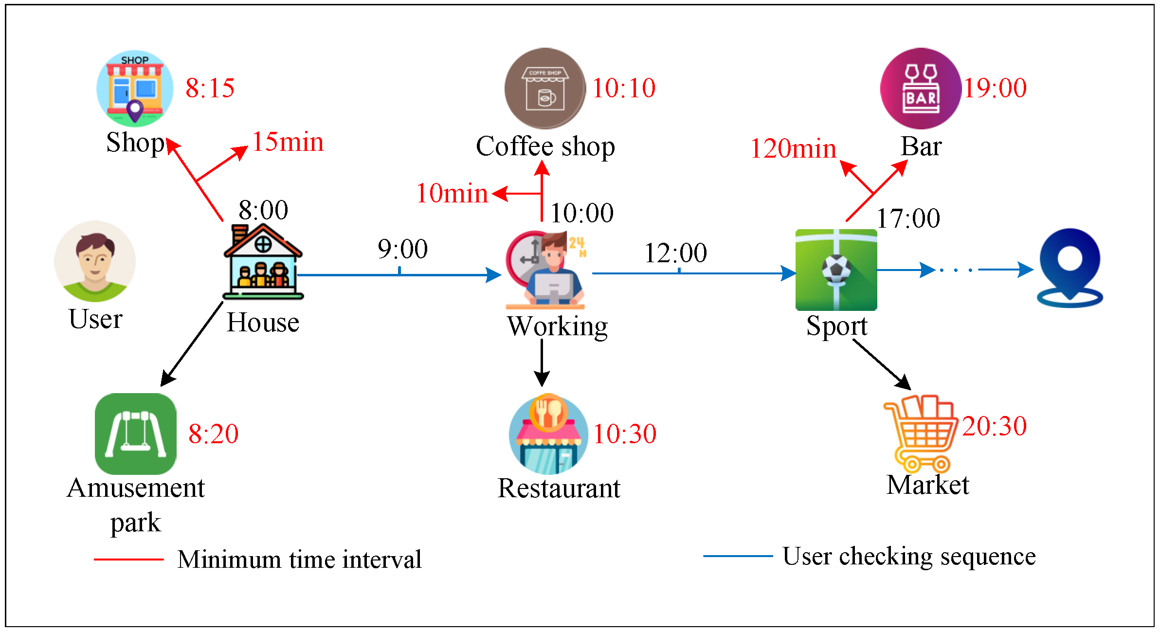
With the wide use of mobile Internet and location-based services, location-based social networks continue to grow and generate large-scale check-in trajectory data. This trend promotes the rapid development of next POI recommendation systems based on check-in sequences. Next POI recommendation supports destination recommendation, travel assistance, and context-aware services, which are closely related to urban-mobility services, cultural tourism, and urban governance in smart cities. These practical needs further drive the development of this research area. However, next POI recommendation still faces several unresolved challenges in real-world scenarios. These challenges mainly arise from the spatio-temporal heterogeneity and uncertainty of user mobility in LBSN data, and they are also affected by data sparsity and privacy constraints. First, check-in time intervals are usually uneven, and the same user often shows stable but fine-grained differences in mobility rhythms across work and leisure periods. When time is only coarsely discretized or ignored, models often fail to capture such intra-day changes adequately [1,2]. Second, user trajectories often contain multi-location co-occurrence patterns and higher-order dependencies. For example, multiple locations may frequently appear together within a certain period, or stable location groups may form within a specific spatial range. Such structural information is difficult to fully represent with only pairwise transition relations. Third, effective structural priors become more important for sparse trajectories and cold-start users. Without structural constraints such as time-aware geographical reachability and fine-grained contextual information, recommendation results may become less targeted and tend to be unstable or overly concentrated when the candidate space is large. Figure 1 gives an intuitive example. During working hours, a user may move between locations within a short time interval. For instance, on a workday, the transition from a workplace to a coffee shop reflects a continuous and compact activity pattern. By contrast, the transition from a sports venue to an entertainment venue after work often involves a more evident time interval. This observation suggests that richer structural representations are needed to support more robust modeling so that the model can learn these behavioral patterns more effectively.

Existing studies have attempted to address the above challenges from different perspectives. Early methods based on matrix factorization and Markov-chain modeling mainly aim to learn stable user preferences and local transition regularities from sparse interactions [3,4]. These methods provide simple and interpretable solutions for preference learning and adjacent transition modeling, but they are usually insufficient for capturing nonlinear mobility dynamics, uneven temporal intervals, and complex spatio-temporal dependencies. To better model trajectory evolution, deep sequential models further introduce recurrent networks, attention mechanisms, and Transformer-style architectures. These methods improve the representation of long-range dependencies and can incorporate spatial or temporal contexts into the sequence modeling process [5,6,7]. They partially respond to the problem of irregular mobility rhythms and long-term behavioral dependency. However, most sequential models still rely heavily on individual historical trajectories. When user trajectories are short or sparse, the learned representations may become unstable because relational information among POIs is not sufficiently propagated. Recent graph- and hypergraph-based methods, therefore, introduce structural learning to supplement structural priors through graph or hypergraph propagation [8,9,10,11]. Such methods are effective for modeling POI relations, high-order co-occurrence patterns, and sparse-trajectory scenarios, and they can alleviate cold-start issues to some extent. Nevertheless, existing structural frameworks often treat temporal information as coarse features or model only a single temporal cue. They still lack a unified mechanism to jointly incorporate uneven time-interval constraints, hourly intra-day regularities, geographic reachability, and higher-order structural propagation. This limitation leaves room for further improvement, especially in time-sensitive real-world scenarios with sparse trajectories. To this end, this paper proposes ASTHN, an Adaptive Spatial-Temporal Hypergraph Network. ASTHN constructs fine-grained spatio-temporal contextual views based on minimum time intervals, spatial proximity, and hourly preferences, and organizes POIs into a hypergraph structure to obtain richer higher-order relational representations and structural priors. It then adopts a context-adaptive fusion mechanism to align and integrate multi-source spatio-temporal signals so that the model can adapt to heterogeneous dependencies across users and time periods. Finally, ASTHN introduces a sequential modeling module with spatio-temporal gates to capture trajectory dynamics, and applies temperature scaling at the output layer to alleviate overly sharp distributions, thereby improving the coverage and stability of recommendation lists. The main contributions of this paper are summarized as follows:

• We propose a unified hypergraph modeling framework that explicitly encodes three types of fine-grained spatio-temporal contexts, including minimum time intervals, spatial proximity, and hourly preferences, as complementary views to enhance structural priors and representation robustness under sparse trajectories.
• We design a context-adaptive fusion mechanism to align and dynamically integrate multi-source spatio-temporal signals, enabling the model to better capture preference differences and contextual dependencies across users and time periods.
• We introduce a sequential modeling module with spatio-temporal gates and a temperature-scaled output strategy, which preserves the ability to model trajectory dynamics while alleviating overly concentrated output distributions and improving the usability and stability of recommendation results.
• We conduct systematic experiments and analyses on two real-world Foursquare datasets, demonstrating that the proposed method achieves better performance gains and favorable training efficiency compared with representative baselines.

2. Related Work

Early studies on POI recommendation and next POI recommendation largely follow classical recommender systems and sequential transition modeling. They focus on learning stable preferences from sparse interactions and capturing local sequential transition patterns. The matrix factorization method proposed by Koren et al. represents long-term preferences by learning latent factors of users and POIs. It is simple to implement and easy to interpret, but its ability to model sequential dynamics and complex spatio-temporal dependencies is limited [3]. Markov-chain-based methods model visit behavior as a state transition process and directly capture short-term dependencies between adjacent visits. However, transition estimation is often unstable when trajectories are sparse, the transition space is large, or cold-start users are involved [12,13]. Rendle et al. propose FPMC, which combines personalized Markov transitions with latent preferences and alleviates the instability caused by sparse transitions to some extent [4]. Feng et al. further propose PRME, which uses metric learning to jointly consider sequential information, individual preferences, and geographical influence, thereby improving ranking quality [14]. Sun et al. propose LSTPM, which incorporates long- and short-term preferences and geographical factors into a unified framework to better capture preference evolution and geographical reachability [15]. Overall, classical methods emphasize long-term preferences, short-term transitions, and geographical constraints. However, they usually lack a unified modeling ability for nonlinear spatio-temporal interactions, fine-grained temporal regularities, and propagable structural priors. This limitation motivates the introduction of deep models and structural learning methods for this task.

2.1. Sequential Next POI Recommendation

With the development of deep learning, sequential modeling is widely used to capture the dynamic evolution of preferences along user trajectories. Liu et al. propose an RNN-based next-location prediction model that incorporates spatial and temporal contexts into the recurrent process, thereby enhancing the modeling of trajectory dynamics [5]. In next POI recommendation, spatio-temporal contexts are often explicitly injected into the sequential update mechanism. Zhao et al. propose STGN, which introduces time gates and distance gates into the gating structure. This design enables the model to perceive time intervals and spatial displacements between adjacent visits, improving its ability to model irregular mobility rhythms [16]. Wu et al. propose PLSPL, which enhances the stability of sequential representations by decomposing long- and short-term preferences and helps distinguish recent preferences from long-term interests [17].

To better capture non-adjacent interactions and long-range dependencies, self-attention mechanisms are introduced into trajectory sequence modeling. Luo et al. propose STAN, which aggregates key historical visits through spatio-temporal attention and helps alleviate the information insufficiency caused by relying only on adjacent transitions [6]. Xu et al. propose STTF-Recommender, which uses attention matching in a multi-layer Transformer to mine spatio-temporal relations among visited locations for next POI prediction [7]. These studies show that self-attention mechanisms can effectively improve long-range dependency modeling and key historical-segment selection. Therefore, they are often used as mature sequential interaction components in subsequent studies to enhance trajectory representations.

Some studies further strengthen sequential signals from the perspectives of user relations and contextual preferences. Fang et al. propose URPI-GRU, which incorporates user relations and preference information into the gated recurrent process to enhance sequential representations and improve next POI recommendation [18]. Wang et al. propose CCDSA, which jointly models sequential dependencies and preference differences through context-aware and category-aware dual self-attention, thereby improving the specificity of next POI prediction [19]. Overall, deep sequential models are effective in modeling trajectory dynamics. However, they still mainly rely on single-user histories, while propagable structural priors remain insufficient. In sparse-trajectory and cold-start scenarios, models that depend only on sequential recurrence may still suffer from unstable representations and limited generalization. This motivates further research on structural learning to compensate for the lack of structural priors.

2.2. Graph- and Hypergraph-Based Next POI Recommendation

Structural learning provides another important path for next POI recommendation. Its core goal is to mine relations and structural signals among POIs through propagation, thereby improving representation robustness in sparse and cold-start scenarios. Graph neural networks can naturally represent user–POI interaction relations and obtain more robust node representations through neighborhood aggregation. Wu et al. propose HAGCN, which constructs a user–POI bipartite graph and combines adaptive temporal patterns with graph convolutional propagation to improve representation-learning quality under sparse data [20]. Based on graph structures, some studies further attempt to disentangle sequential factors from geographical factors to reduce the confounding effect between geographical proximity and sequential transitions. Qin et al. propose DisenPOI, which improves representation interpretability and generalization by separately modeling sequential transitions and geographical proximity [9]. Zuo et al. propose GUGEN, which constructs a global location relation graph and individual user-history graphs, and integrates global and user-specific views to improve recommendation performance in sparse and cold-start scenarios [10]. Yang et al. propose GETNext, which combines a trajectory-flow map with a graph-enhanced Transformer to improve prediction under sparse trajectories and trajectory-level structural patterns, and it may alleviate cold-start issues to some extent [8]. For structural robustness and factor disentanglement, Wang et al. propose DRAN, which separates influencing factors through graph-representation disentanglement and reduces confounding interference, thereby enhancing representation robustness in sparse scenarios [21]. Wang et al. propose GSTN, which introduces a graph-enhanced spatio-temporal network to jointly model structural propagation and user spatio-temporal dependencies, further improving generalization under sparse data [22].

Compared with ordinary graph structures, hypergraphs connect multiple POIs through one hyperedge, making them more suitable for modeling higher-order relations such as multi-location co-occurrence and stage-specific location groups. Yan et al. propose STHGCN, which adopts spatio-temporal hypergraph learning and Transformer-style fusion to jointly encode higher-order structures and spatio-temporal contexts [11]. Lai et al. propose DCHL, which further enhances hypergraph-representation learning through disentanglement and contrastive learning, improving the modeling of higher-order relations [23]. Lai et al. also propose MSTHN, which uses multi-view hypergraph construction and spatial-temporal enhancement to improve next POI recommendation under sparse trajectories [24]. An et al. propose MvStHgL, which combines periodic interests with multi-view hypergraph learning and provides a useful perspective for jointly representing periodic preferences and higher-order structures [25]. These studies indicate that hypergraph neural networks have advantages in terms of modeling higher-order structural dependencies and can provide richer and more structured prior information for sparse trajectories. However, structural methods still often treat temporal contexts in a less unified way. Temporal information may be simplified into coarse-grained features, or it may be insufficiently coupled with geographical reachability constraints. As a result, these methods may fail to explain different migration rhythms across intra-day stages in a unified manner.

2.3. Fine-Grained Temporal Context for Next POI Recommendation

Fine-grained temporal context is usually reflected in uneven time intervals, intra-day stage-specific preferences, and explicit timestamp constraints. Li et al. propose an uneven-interval-aware self-attention model that introduces uneven spatio-temporal interval information into attention computation, thereby improving dependency modeling for irregular check-in sequences [1]. Duan et al. propose TSCAN, which uses the next timestamp as a query signal and retrieves matched historical patterns through cross-attention to capture migration regularities under temporal constraints [26]. Xu et al. propose TAPT, which jointly predicts the next POI and the explicit timestamp, and strengthens temporal constraints through structured temporal encoding [27]. To further enhance uneven-interval constraints, Zhang et al. propose GESTIAN, which explicitly models spatio-temporal intervals and combines them with a global trajectory-flow graph to learn general behavioral patterns, thereby improving next POI recommendation under uneven-interval constraints and alleviating cold-start effects [28]. He et al. propose ImNext, which jointly captures interval features and user states through irregular-interval attention and multi-task learning, strengthening time-sensitive modeling for irregular check-in sequences [29]. Beyond time intervals, semantic information and external relations are also used to enhance the modeling of time-sensitive preferences. For example, Tian et al. propose a method that jointly learns preference and semantic representations to describe intra-day preference differences in a more fine-grained manner [2]. The contextual knowledge graph-learning method proposed by Zhou et al. provides a direction for supplementing semantic and relational information in sparse scenarios [30]. Overall, the trend toward explicit temporal context modeling is becoming increasingly clear. However, the collaborative use of different fine-grained temporal cues, and their unified coupling with structural propagation and trajectory dynamic modeling, still require further exploration.

2.4. Summary and Comparison to ASTHN

Table 1. High-level design comparison of representative next POI recommendation methods. The symbol ✓ indicates that the corresponding factor is explicitly modeled as a core component, while × indicates that it is not explicitly modeled. “Interval” denotes explicit modeling of uneven time intervals, and “hourly” denotes explicit modeling of hourly intra-day regularities. Blank entries in the Category column inherit the category from the nearest preceding non-blank entry.

Category	Method	Structure	Geographic Modeling	Temporal Cue
Traditional/metric	MF [3]	–	×	×
	FPMC [4]	–	×	×
	PRME [14]	–	✓	×
Sequential	LSTPM [15]	–	✓	×
	STGN [16]	–	✓	Interval
	PLSPL [17]	–	×	×
Attention/Transformer	STAN [6]	–	✓	Interval
	STTF [7]	–	✓	Coarse time
	GETNext [8]	Graph	✓	Coarse time
Graph/hypergraph	DisenPOI [9]	Graph	✓	×
	GUGEN [10]	Graph	✓	×
	STHGCN [11]	Hypergraph	✓	Coarse time
	MSTHN [24]	Hypergraph	✓	Coarse time
	DCHL [23]	Hypergraph	×	×
Proposed method	ASTHN (Ours)	Hypergraph	✓	Interval + hourly

summarizes representative next POI recommendation methods from three aspects: structure type, geographic modeling, and temporal cue. Structure type indicates whether graph-based or hypergraph-based propagation is used. Geographic modeling indicates whether geographic information, such as distance, spatial proximity, or geographic relations, is explicitly used as a core component. Temporal cue distinguishes whether a method models coarse temporal information, uneven time intervals, or hourly intra-day regularities.

From Table 1, traditional methods mainly learn preferences or adjacent transition patterns from sparse interactions. However, they usually do not explicitly model structural propagation, geographic reachability, or fine-grained temporal constraints. Therefore, they are more likely to suffer from unstable representations or insufficient recommendation specificity in short-trajectory and cold-start scenarios [3,4]. Deep sequential models use recurrent mechanisms to capture the dynamic change in preferences along user trajectories, and they may incorporate geographic context to enhance local reachability modeling [15,16]. Nevertheless, this line of work still mainly relies on single-user histories and lacks propagable structural priors to compensate for missing relational information under sparse and cold-start conditions.

Attention- and Transformer-based methods enhance the ability to capture non-adjacent dependencies and long-range correlations, and they are often combined with geographic context to improve the plausibility of next POI prediction [6,7]. However, in the temporal dimension, many of these methods still rely on coarse-grained temporal features or a single temporal cue. They are, therefore, less able to jointly cover uneven-interval migration constraints and hourly intra-day regularities, especially in scenarios where behavior changes clearly across different daily stages.

Graph- and hypergraph-based methods supplement structural priors through structural propagation. They can alleviate representation instability caused by sparsity and cold-start issues to some extent, and they may incorporate geographic relations as spatial constraints into structural encoding [8,9,10,11]. However, existing structural methods often treat temporal contexts in a fragmented manner. On the one hand, temporal information is often simplified into coarse-grained features. On the other hand, even when temporal cues are introduced, they are often not jointly coupled with geographic-reachability constraints to form fine-grained constraints on the same migration decision. As a result, it remains difficult to explain differentiated rhythms such as compact short-interval transitions and sparse cross-period transitions within a unified framework.

To address these limitations, ASTHN explicitly integrates three complementary spatio-temporal contexts within a unified framework. It uses minimum time intervals to characterize the lower bound of migration rhythms, spatial proximity to characterize geographic reachability constraints, and hourly preferences to characterize intra-day stage-specific interest transition regularities. Based on these contexts, ASTHN constructs a multi-view hypergraph structure to learn more robust structural priors. This design allows structural propagation to be jointly modulated by geographic constraints and fine-grained temporal cues, thereby improving the stability of POI representations and the usability of recommendation results in sparse-trajectory and time-sensitive scenarios.

3. Problem Definition

• Check-in sequence: Let $\mathcal{U}$ denote the set of users and let $\mathcal{V}$ denote the set of POIs. For a user $u\in \mathcal{U}$, the check-in sequence is denoted by $S^u={\left\{s_t^u\right\}}_{t=1}^T$, where $s_t^u=(v_t^u,{\tau }_t^u)$. Here, $v_t^u\in \mathcal{V}$ denotes the POI visited at step t, and ${\tau }_t^u$ denotes the corresponding timestamp. The hour index is defined as $h_t^u=\mathrm{hour}({\tau }_t^u)$.
• Minimum time interval: Let ${\mathcal{V}}_u\subseteq \mathcal{V}$ denote the set of POIs visited by user u. Let $T_i^u={\left\{t_k^i\right\}}_{k=1}^{n_i}$ denote the visit times of POI i for user u, sorted in ascending order. The minimum positive time-interval matrix ${\mathbf{D}}^{\Delta t}\in {\mathbb{R}}^{|{\mathcal{V}}_u|\times |{\mathcal{V}}_u|}$ is defined as

  $$D_{ij}^{\Delta t}=\left\{\begin{array}{cc}\underset{k}{min}{\displaystyle \frac{t_{k+1}^i-t_k^i}{60}},\hfill & i=j,n_i\ge 2,\hfill \\ \underset{\begin{array}{c}t\in T_i^u,t^{\prime }\in T_j^u\\ t^{\prime }>t\end{array}}{min}{\displaystyle \frac{t^{\prime }-t}{60}},\hfill & i\ne j,\exists t^{\prime }>t,\hfill \\ 0,\hfill & \mathrm{otherwise},\hfill \end{array}\right.$$

  (1)

  where the unit is hours.
• Geographic distance: Given two POIs with latitude and longitude $({\mathrm{lat}}_1,{\mathrm{lon}}_1)$ and $({\mathrm{lat}}_2,{\mathrm{lon}}_2)$, the Haversine distance is defined as

  $$d_{12}=2Rarcsin\left(\sqrt{{sin}^2\left({\displaystyle \frac{\Delta \mathrm{lat}}{2}}\right)+cos({\mathrm{lat}}_1)cos({\mathrm{lat}}_2){sin}^2\left({\displaystyle \frac{\Delta \mathrm{lon}}{2}}\right)}\right),$$

  (2)

  where $R=6371$ km, $\Delta \mathrm{lat}={\mathrm{lat}}_2-{\mathrm{lat}}_1$, and $\Delta \mathrm{lon}={\mathrm{lon}}_2-{\mathrm{lon}}_1$.
• Hourly pattern: For user u, the hourly frequency vector is ${\mathbf{c}}^u\in {\mathbb{R}}^{24}$ and is defined as

  $$c_h^u={\displaystyle \sum _{t=1}^T}\mathbb{I}(h_t^u=h),h\in \{0,\dots ,23\}.$$

  (3)
  The normalized hourly weight vector is ${\mathbf{w}}^u\in {\mathbb{R}}^{24}$, where $w_h^u=c_h^u/T$.
• Next POI recommendation: Given $S^u$, the task is to predict the next POI $v_{T+1}^u$ and output a Top-K ranked list. In this work, the candidate set is restricted to ${\mathcal{V}}_u$.

4. Proposed Method

4.1. Framework Overview

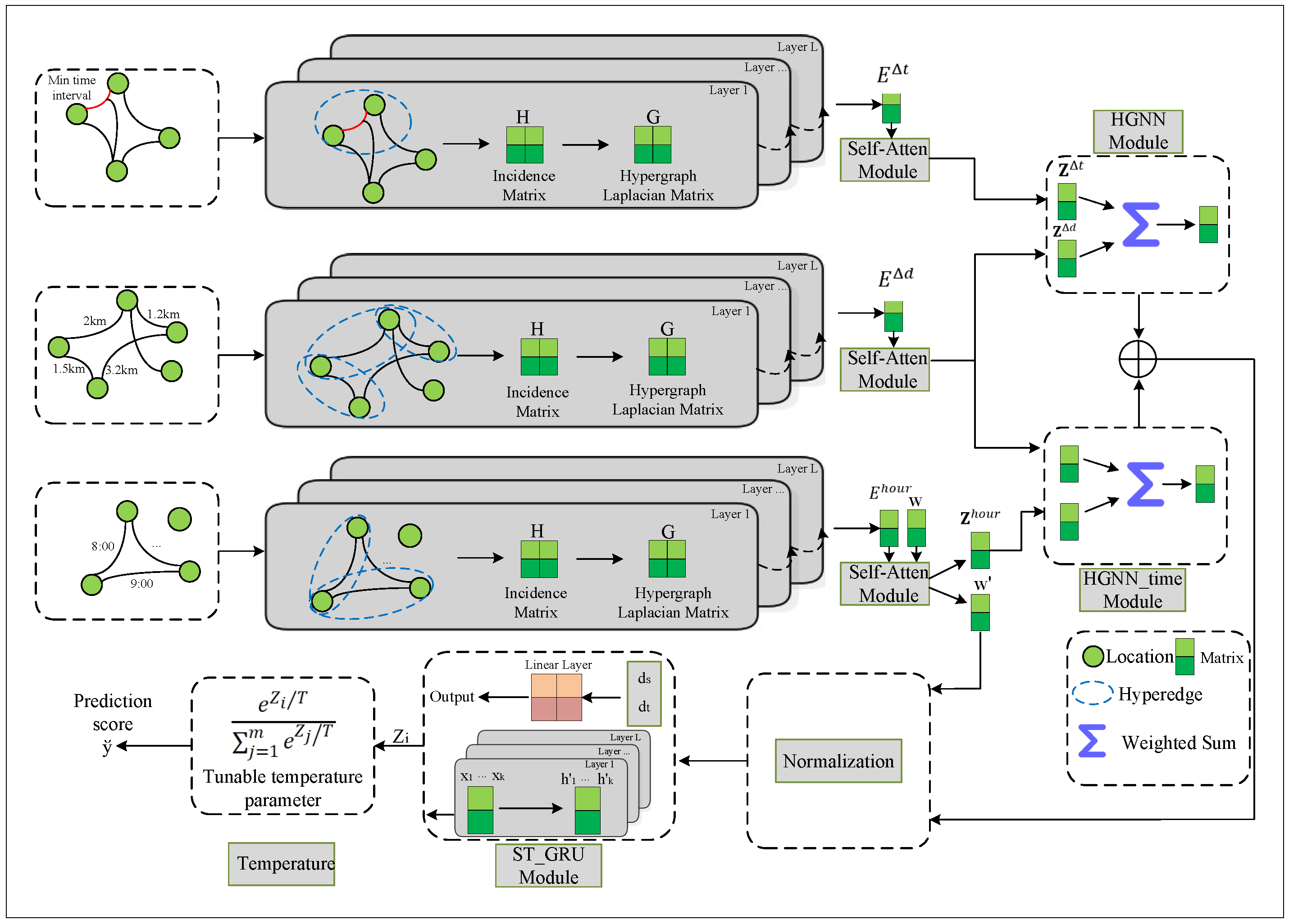
Next POI recommendation with hypergraph neural networks is promising, but it remains challenging because human mobility exhibits complex temporal dependence. Coarse temporal features often fail to capture fine-grained temporal habits. ASTHN addresses this issue by combining time-constrained geographic reachability with fine-grained hourly preference in a unified hypergraph framework. Figure 2 shows the overall architecture.

In check-in-trajectory modeling, context can be derived from several sources, such as sequential transitions, geographic reachability, time intervals, and daily periodicity. External signals such as semantics or social links can also be used, but they often require extra data and may be inconsistent across platforms. ASTHN focuses on three views that are stable and directly available from check-ins. Minimum time interval captures a lower bound on movement rhythm. Spatial proximity captures geographic reachability. Hourly preference captures stage-specific changes in interest over a day. These views are complementary and can provide structural priors under sparse trajectories.

The model first extracts three types of features, minimum time interval, spatial distance, and hourly pattern. Hypergraph encoders then learn view-specific POI representations. A context-adaptive fusion module aligns and combines signals from different views. Finally, an ST-GRU models sequence dynamics with spatio-temporal gates, and temperature scaling smooths the final score distribution.

4.2. Fine-Grained Spatio-Temporal-Context Hypergraph Construction

We convert each user check-in history into three spatio-temporal-context hypergraphs so that higher-order propagation can be performed on POI nodes. POIs are treated as vertices, and three context views are used: minimum time interval, spatial proximity, and hourly preference. These views provide complementary structural priors under sparse trajectories.

4.2.1. Time-Interval Hypergraph

For each user u, we first derive a binary time-reachability matrix ${\mathbf{B}}^{\Delta t,u}\in {\{0,1\}}^{|{\mathcal{V}}_u|\times |{\mathcal{V}}_u|}$ from the minimum positive time-interval matrix ${\mathbf{D}}^{\Delta t}$. A pair $(i,j)$ is connected if $D_{ij}^{\Delta t}>0$. A simple construction is

$$B_{ij}^{\Delta t,u}=\left\{\begin{array}{cc}1,\hfill & D_{ij}^{\Delta t}>0,\hfill \\ 0,\hfill & \mathrm{otherwise}.\hfill \end{array}\right.$$

(4)

To match the hypergraph propagation form, we define the time-interval hyperedge set as ${\mathcal{E}}_u^{\Delta t}=\{e_j^{\Delta t}\mid v_j\in {\mathcal{V}}_u\}$, where each hyperedge $e_j^{\Delta t}$ is anchored at POI j and connects all POIs i that satisfy $B_{ij}^{\Delta t,u}=1$, i.e., $e_j^{\Delta t}=\{v_i\in {\mathcal{V}}_u\mid B_{ij}^{\Delta t,u}=1\}$. The corresponding incidence matrix is ${\mathbf{H}}^{\Delta t,u}\in {\{0,1\}}^{|{\mathcal{V}}_u|\times |{\mathcal{E}}_u^{\Delta t}|}$ with elements $H_{i,e_j^{\Delta t}}^{\Delta t,u}=B_{ij}^{\Delta t,u}$. Since one anchored hyperedge is constructed for each POI, $|{\mathcal{E}}_u^{\Delta t}|=|{\mathcal{V}}_u|$, the matrix can be square in shape while still representing vertex–hyperedge incidence. This construction captures reachability under temporal constraints.

4.2.2. Spatial-Proximity Hypergraph

For each user u, spatial relations are computed on the user-specific POI set ${\mathcal{V}}_u$. A spatial threshold ${\delta }_u$ is estimated with k-nearest neighbors so that the construction is less sensitive to city scale and local density. Let ${\mathcal{N}}_i^u$ denote the set of k nearest neighbors of POI i within ${\mathcal{V}}_u$. The threshold is defined as

$${\delta }_u={\displaystyle \frac{1}{|{\mathcal{V}}_u|}}\sum _{i\in {\mathcal{V}}_u}\left({\displaystyle \frac{1}{k}}\sum _{j\in {\mathcal{N}}_i^u}{d}_{ij}\right).$$

(5)

A weighted adjacency matrix ${\mathbf{A}}^u\in {\mathbb{R}}^{|{\mathcal{V}}_u|\times |{\mathcal{V}}_u|}$ is then constructed with a Gaussian kernel:

$$A_{ij}^u=\left\{\begin{array}{cc}exp\left(-{\displaystyle \frac{d_{ij}^2}{2{\sigma }^2}}\right),\hfill & d_{ij}\le {\delta }_u,\hfill \\ 0,\hfill & d_{ij}>{\delta }_u.\hfill \end{array}\right.$$

(6)

To keep the formulation consistent across views, we convert ${\mathbf{A}}^u$ into a spatial hypergraph. We define the spatial hyperedge set as the formulation consistent across views, we convert ${\mathbf{A}}^u$ into a spatial hypergraph. ${\mathcal{E}}_u^{\Delta d}=\{e_j^{\Delta d}\mid v_j\in {\mathcal{V}}_u\}$, where $e_j^{\Delta d}=\{v_i\in {\mathcal{V}}_u\mid A_{ij}^u>0\}$. The spatial incidence matrix is ${\mathbf{H}}^{\Delta d,u}\in {\{0,1\}}^{|{\mathcal{V}}_u|\times |{\mathcal{E}}_u^{\Delta d}|}$, with elements $H_{i,e_j^{\Delta d}}^{\Delta d,u}=\mathbb{I}(A_{ij}^u>0)$. This construction suppresses distant noisy connections while preserving locally reachable structure.

4.2.3. Hourly Preference Hypergraph

For each user u, a user-specific hourly preference matrix is constructed as ${\mathbf{P}}^u\in {\{0,1\}}^{|{\mathcal{V}}_u|\times 24}$. The element $P_{i,h}^u=1$ if user u visits POI i at hour h. Each hour h defines a hyperedge that connects all POIs visited during that hour. The corresponding hourly incidence matrix is denoted by ${\mathbf{H}}^{hour,u}$. The hourly weight vector ${\mathbf{w}}^u\in {\mathbb{R}}^{24}$ describes activity intensity at each hour and is used later as a time-aware hyperedge-weight prior.

4.2.4. View-Specific Structural Encoding

For user u, the three hypergraphs are denoted by ${\mathbf{H}}^{\Delta t,u}$, ${\mathbf{H}}^{\Delta d,u}$, and ${\mathbf{H}}^{hour,u}$. We use a shared initial POI embedding matrix ${\mathbf{E}}^{(0)}\in {\mathbb{R}}^{\left|\mathcal{V}\right|\times d}$ and extract a user-specific sub-table ${\mathbf{E}}_u^{(0)}={\mathbf{E}}^{(0)}[{\mathcal{V}}_u,:]\in {\mathbb{R}}^{|{\mathcal{V}}_u|\times d}$ as the input of structure encoding. We apply an L-layer HGNN to each view. The hypergraph convolution is written as

$${\mathbf{E}}^{(l+1)}=\sigma \left({\mathbf{D}}_v^{-{\displaystyle \frac{1}{2}}}\mathbf{H}\mathbf{W}{\mathbf{D}}_e^{-1}{\mathbf{H}}^{\top }{\mathbf{D}}_v^{-{\displaystyle \frac{1}{2}}}{\mathbf{E}}^{(l)}{\mathrm{\Theta }}^{(l)}\right),$$

(7)

where $\mathbf{H}$ is an incidence matrix, $\mathbf{W}$ is a diagonal hyperedge-weight matrix, ${\mathbf{D}}_v$ and ${\mathbf{D}}_e$ are the degree matrices of vertices and hyperedges, and ${\mathrm{\Theta }}^{(l)}$ is a learnable parameter. The view-specific outputs are denoted by ${\mathbf{E}}^{\Delta t,u}$, ${\mathbf{E}}^{\Delta d,u}$, and ${\mathbf{E}}^{hour,u}$ in ${\mathbb{R}}^{|{\mathcal{V}}_u|\times d}$. These representations are then passed to the alignment and fusion modules.

4.3. Spatio-Temporal-Context Adaptive Fusion

The fusion module combines the representations of time interval, spatial proximity, and hourly preference, while also using the hourly weight prior. Under sparse and noisy trajectories, fixed concatenation or fixed weighting can easily introduce bias. ASTHN, therefore, uses a two-stage adaptive fusion scheme. The first stage recalibrates each view with self-attention. The second stage arranges the three views into two complementary propagation paths. Spatial proximity serves as a shared reachability constraint in both paths. A gating mechanism then combines the outputs of the two paths into the final POI embedding matrix, which is used directly by the prediction module.

Let the three view-specific matrices be ${\mathbf{E}}^{\Delta t,u}$, ${\mathbf{E}}^{\Delta d,u}$, and ${\mathbf{E}}^{hour,u}$. Each view is first mapped into a shared latent space:

$${\mathbf{Z}}^k=\mathrm{Norm}\left({\mathbf{E}}^{k,u}{\mathbf{W}}_k+{\mathbf{b}}_k\right),k\in \{\Delta t,\Delta d,hour\},$$

(8)

where ${\mathbf{W}}_k$ and ${\mathbf{b}}_k$ are learnable parameters, and $\mathrm{Norm}(·)$ denotes a normalization operator. We use a simple min–max normalization for a matrix $\mathbf{X}$:

$${\mathbf{X}}_{norm}={\displaystyle \frac{\mathbf{X}-min(\mathbf{X})}{max(\mathbf{X})-min(\mathbf{X})}}.$$

(9)

Self-attention is then applied to each aligned view:

$${\tilde{\mathbf{Z}}}^k=\mathrm{Attn}({\mathbf{Z}}^k)=\mathrm{softmax}\left({\displaystyle \frac{{\mathbf{Q}}^k{({\mathbf{K}}^k)}^{\top }}{\sqrt{d}}}\right){\mathbf{V}}^k,{\mathbf{Q}}^k={\mathbf{Z}}^k{\mathbf{W}}_Q^k,{\mathbf{K}}^k={\mathbf{Z}}^k{\mathbf{W}}_K^k,{\mathbf{V}}^k={\mathbf{Z}}^k{\mathbf{W}}_V^k.$$

(10)

This step highlights the most important interactions within each view. Next, we build two propagation paths. One combines time interval with spatial proximity. The other combines hourly preference with spatial proximity and further uses the hourly weight prior ${\mathbf{w}}^u$. To avoid fixed weighting, each path uses node-wise adaptive fusion to combine its two inputs. For each POI node i, the time–geo path computes

$$\left[{\alpha }_i^{\Delta t},{\alpha }_i^{\Delta d}\right]=\mathrm{softmax}\left({\mathbf{W}}_{tg}\left[{\tilde{\mathbf{Z}}}_i^{\Delta t};{\tilde{\mathbf{Z}}}_i^{\Delta d}\right]+{\mathbf{b}}_{tg}\right),{\mathbf{U}}_i^{tg}={\alpha }_i^{\Delta t}{\tilde{\mathbf{Z}}}_i^{\Delta t}+{\alpha }_i^{\Delta d}{\tilde{\mathbf{Z}}}_i^{\Delta d},$$

(11)

and the hour–geo path computes ${\mathbf{U}}_i^{hg}$ in the same way by replacing $\Delta t$ with $hour$ and using its own parameters $({\mathbf{W}}_{hg},{\mathbf{b}}_{hg})$. Each path then performs hypergraph propagation using the corresponding incidence matrices and produces a structure-enhanced POI representation, denoted by ${\mathbf{E}}^{tg,u}$ and ${\mathbf{E}}^{hg,u}$ in ${\mathbb{R}}^{|{\mathcal{V}}_u|\times d}$. In the hour–geo path, the hourly weight vector ${\mathbf{w}}^u$ is used as the hyperedge-weight prior of the hourly hypergraph so that propagation is more sensitive to the active hours of user u.

A gated fusion then produces the final POI embedding matrix:

$$\mathbf{g}=\sigma \left(\left[{\mathbf{E}}^{tg,u};{\mathbf{E}}^{hg,u}\right]{\mathbf{W}}_g+{\mathbf{b}}_g\right),{\mathbf{E}}^{f,u}=\mathbf{g}\odot {\mathbf{E}}^{tg,u}+(1-\mathbf{g})\odot {\mathbf{E}}^{hg,u},$$

(12)

where $\mathbf{g}\in {\mathbb{R}}^{|{\mathcal{V}}_u|\times d}$. This gate allows different nodes to rely on the contextual source that is more informative for them. The resulting matrix ${\mathbf{E}}^{f,u}$ is used as the POI embedding lookup table in the prediction module.

4.4. Spatio-Temporal Gated Sequential Prediction with Temperature Scaling

The prediction module models dynamic movement and produces the final ranked list. It maps a user trajectory to an embedding sequence and injects time-interval and distance signals through spatio-temporal gates. Temperature scaling is then used at the output layer to reduce overly sharp distributions.

The final POI embedding matrix is ${\mathbf{E}}^{f,u}\in {\mathbb{R}}^{|{\mathcal{V}}_u|\times d}$. The sequence embedding is defined as

$${\mathbf{x}}_t^u={\mathbf{E}}^{f,u}[v_t^u,:]\in {\mathbb{R}}^d,{\mathbf{X}}^u={\left\{{\mathbf{x}}_t^u\right\}}_{t=1}^T.$$

(13)

A preprocessing step constructs a time-interval matrix ${\mathbf{D}}_t^u\in {\mathbb{R}}^{T\times T}$ and a distance matrix ${\mathbf{D}}_s^u\in {\mathbb{R}}^{T\times T}$. These matrices describe pairwise temporal gaps and geographic distances within the sequence. We then extract a gate sequence from adjacent transitions:

$$d_t^u\left[t\right]={\mathbf{D}}_t^u[t-1,t],d_s^u\left[t\right]={\mathbf{D}}_s^u[t-1,t],t=2,\dots ,T,$$

(14)

and the boundary term is set to zero at $t=1$.

Two gate vectors are computed and applied to the input embedding:

$${\mathbf{g}}_t^{\Delta t}=\sigma ({\mathbf{W}}_{\Delta t}{d}_t^u\left[t\right]+{\mathbf{U}}_{\Delta t}{\mathbf{x}}_t^u),{\mathbf{g}}_t^{\Delta d}=\sigma ({\mathbf{W}}_{\Delta d}{d}_s^u\left[t\right]+{\mathbf{U}}_{\Delta d}{\mathbf{x}}_t^u),$$

(15)

$${\tilde{\mathbf{x}}}_t^u=tanh\left({\mathbf{W}}_h({\mathbf{x}}_t^u\odot {\mathbf{g}}_t^{\Delta t}\odot {\mathbf{g}}_t^{\Delta d})+{\mathbf{b}}_h\right).$$

(16)

With this design, the recurrent update becomes sensitive to both movement rhythm and spatial displacement. A GRU encodes the gated sequence:

$${\mathbf{h}}_t^u=\mathrm{GRU}({\tilde{\mathbf{x}}}_t^u,{\mathbf{h}}_{t-1}^u),t=1,\dots ,T,$$

(17)

where ${\mathbf{h}}_t^u\in {\mathbb{R}}^H$ denotes the hidden state. The final state ${\mathbf{h}}_T^u$ summarizes the current preference. A score vector over candidate POIs is then computed as

$${\mathbf{o}}^u={\mathbf{E}}^{f,u}{\mathbf{W}}_o{\mathbf{h}}_T^u\in {\mathbb{R}}^{|{\mathcal{V}}_u|},$$

(18)

where ${\mathbf{W}}_o\in {\mathbb{R}}^{d\times H}$ aligns the hidden state to the embedding space. Temperature scaling smooths the logits and reduces score over-concentration:

$${\tilde{\mathbf{o}}}^u={\displaystyle \frac{{\mathbf{o}}^u}{T}},{\widehat{\mathbf{y}}}^u=\mathrm{softmax}({\tilde{\mathbf{o}}}^u),T>0.$$

(19)

A smaller T gives a sharper distribution, while a larger T gives a smoother one and can improve coverage. The Top-K POIs are obtained by sorting ${\widehat{\mathbf{y}}}^u$.

5. Experiments

5.1. Datasets

We evaluate the model on two public real-world datasets, Foursquare-NYC and Foursquare-TKY. Each dataset contains roughly ten months of check-in records from 12 April 2012 to 16 February 2013. Each record includes an anonymized user ID, a POI ID with latitude and longitude, a POI category ID, and a timestamp. The latitude and longitude information is also used in the spatial hypergraph construction and the application-oriented case visualization.

Table 2. Dataset statistics.

Dataset	#Users	#POIs	#Check-Ins
Foursquare-NYC	1064	5136	147939
Foursquare-TKY	2245	7872	447571

reports the statistics of the two datasets.

5.2. Settings and Baselines

The model is implemented in PyTorch 1.9.0 with CUDA 11.1 and trained with the Adam optimizer. The learning rate is set to $2\times {10}^{-3}$. Dropout is set to $0.3$ in the main network and to $0.2$ in the GRU. The main hyperparameters are the embedding dimension, the HGNN depth, and the temperature parameter T. According to the hyperparameter analysis, the embedding dimension is set to 64 and the temperature parameter is set to $T=0.5$ in the final model. To reflect the stability of the proposed model, ASTHN is trained and evaluated three times with different random seeds, and its final results are reported as mean ± std.

• MF [3]: This method applies matrix factorization and learns latent vectors for users and POIs.
• FPMC [4]: This method combines matrix factorization with a Markov chain and learns ranking parameters under the BPR framework.
• LSTPM [15]: This model learns long-term and short-term preferences with a non-local structure and a geography-enhanced LSTM for next POI recommendation.
• GETNext [8]: This model targets next POI prediction under sparse data and incorporates trajectory-level mobility patterns.
• PRME [14]: This method learns a personalized ranking-metric embedding and combines sequential signals, user preference, and geographic influence.
• MSTHN [24]: This model jointly considers spatial relations and temporal dynamics for next POI recommendation.
• DCHL [23]: This model uses dual hypergraphs and bi-directional contrastive learning to improve high-order representation learning, and it is included as a representative contrastive-hypergraph baseline.
• DisenPOI [9]: This model disentangles sequential transition and geographic proximity for next POI recommendation.
• GUGEN [10]: This model builds a global location-relation graph and a user-history graph, and then fuses global and user-specific views.
• STHGCN [11]: This model uses a hypergraph to capture higher-order collaborative information across trajectories and fuses spatio-temporal context with a hypergraph Transformer.

5.3. Performance Comparison

We evaluate all methods with two widely used ranking metrics, Recall@k and normalized discounted cumulative gain NDCG@k, where $k\in \{5,10\}$. The overall results are reported in

Table 3. Performance comparison on Foursquare-NYC and Foursquare-TKY. The best baseline in each column is underlined. The proposed model is shown in bold.

Model	Foursquare-NYC				Foursquare-TKY
	Recall@5	Recall@10	NDCG@5	NDCG@10	Recall@5	Recall@10	NDCG@5	NDCG@10
MF	0.0961	0.1522	0.2318	0.2426	0.0701	0.1267	0.2071	0.2327
FPMC	0.2126	0.2970	0.1526	0.1825	0.2045	0.2746	0.1439	0.1547
LSTPM	0.2495	0.2668	0.2425	0.2483	0.2203	0.2703	0.1556	0.1734
GETNext	0.3572	0.3866	0.3113	0.3094	0.2686	0.3282	0.2212	0.2242
PRME	0.2236	0.3105	0.1664	0.1845	0.2278	0.2944	0.1518	0.1789
MSTHN	0.3585	0.4398	0.3109	0.3619	0.3378	0.3933	0.2569	0.2753
DCHL	0.2478	0.3382	0.2903	0.2433	0.1831	0.2674	0.1513	0.1834
DisenPOI	0.3589	0.3831	0.2979	0.3071	0.2692	0.3314	0.2263	0.2332
GUGEN	0.2355	0.3258	0.1970	0.2310	0.1738	0.2573	0.1424	0.1741
STHGCN	0.2119	0.3123	0.1753	0.2142	0.1513	0.2377	0.1274	0.1534
ASTHN	0.3725±0.0124	0.5041±0.0591	0.3184±0.0102	0.3664±0.0042	0.3575±0.0364	0.5396±0.0150	0.2925±0.0214	0.3317±0.0226
Improvement (%)	+3.79	+14.62	+2.28	+1.24	+5.83	+37.20	+13.86	+20.49

The best baseline in each column is underlined, and the proposed model (ASTHN) is shown in bold. ASTHN results are reported as mean ± std over three runs with different random seeds. Other baselines are reported from a single run under the same setting.

.

Table 3 shows that ASTHN achieves the best results on both datasets. ASTHN improves over the best baseline by 3.79% in Recall@5, 14.62% in Recall@10, 2.28% in NDCG@5, and 1.24% in NDCG@10 on NYC. On TKY, the corresponding gains are 5.83%, 37.20%, 13.86%, and 20.49%. These results show that jointly modeling minimum time intervals, geographic reachability, and hourly temporal patterns leads to more accurate next POI recommendation. In addition, the relatively small standard deviations in most metrics indicate that ASTHN maintains stable performance under different random seeds.

The gains come from three main sources. First, ASTHN builds multi-view hypergraphs that capture complementary spatio-temporal signals. The time-interval hypergraph reflects movement rhythm and transition constraints between POIs, the geographic hypergraph captures spatial reachability among visited POIs, and the hourly-pattern hypergraph introduces fine-grained intra-day temporal cues. Second, the adaptive fusion module integrates these views according to their contextual relevance, rather than relying on fixed weights. Third, the ST-GRU module models dynamic trajectory evolution with spatio-temporal gates, and the temperature parameter calibrates the sharpness of the output scores.

Compared with traditional methods such as MF and FPMC, ASTHN models complex and dynamic spatio-temporal dependence in a more detailed way. MF only captures static global interactions through low-dimensional latent factors, whereas ASTHN models how user behavior evolves through hypergraph-based structural encoding and sequential dynamics. FPMC combines matrix factorization with a first-order Markov chain and, therefore, includes sequential information, but it is still limited in terms of modeling complex trajectories and does not explicitly encode fine-grained temporal cues such as interval constraints and hourly periodicity.

Compared with methods that combine multiple signals, such as PRME and DisenPOI, ASTHN performs deeper and more structured fusion. PRME combines sequential preference, personal preference, and geographic influence in a unified embedding space, but its treatment of complex spatio-temporal interaction remains relatively shallow. DisenPOI uses sequential transitions and geographic proximity for recommendation, but it does not explicitly model fine-grained temporal dynamics such as interval patterns and daily periodicity. By contrast, ASTHN builds three context hypergraphs for time interval, geographic distance, and hourly pattern, which provide a unified structural representation of multi-source spatio-temporal signals. The ST-GRU module then models spatio-temporal dynamics more thoroughly.

Compared with advanced graph-based methods, including GETNext, MSTHN, GUGEN, STHGCN, and DCHL, ASTHN has clear advantages in terms of integrating fine-grained temporal context with structured propagation and adaptive fusion. GETNext combines graph structure with sequential information, but its modeling of fine-grained temporal preference remains limited. MSTHN emphasizes temporal dynamics and spatial modeling, but it is less effective at jointly modeling higher-order relations with explicit fine-grained temporal cues. GUGEN combines global and user-specific graphs, but its graph structure is less expressive for complex higher-order relations in trajectories. STHGCN introduces hypergraphs to capture higher-order collaborative information, but it does not jointly emphasize minimum interval constraints and hourly periodicity in a unified and adaptive manner. DCHL uses dual hypergraphs and contrastive learning to model higher-order interaction, but it does not focus on fine-grained spatio-temporal-context modeling for next POI prediction. Taken together, these comparisons support the effectiveness of ASTHN.

5.4. Ablation Study

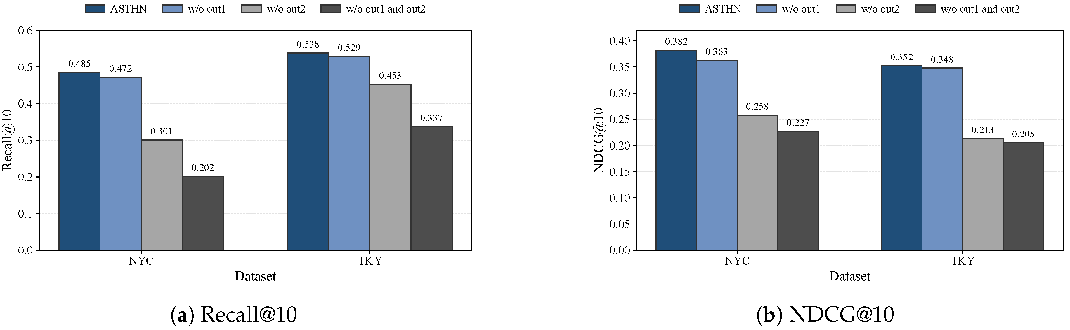
To examine the contribution of each component in ASTHN, we conducted ablation experiments on both NYC and TKY, as shown in Figure 3. The variant w/o out1 and out2 removes both the time-interval branch and the hourly-preference branch and replaces the corresponding fusion process with random embedding encoding. The variant w/o out1 removes the time-interval branch and keeps only the hourly-preference branch. The variant w/o out2 removes the hourly-preference branch and keeps only the time-interval branch. The results on Recall@10 and NDCG@10 show that both the time-interval modality and the hourly-preference modality are essential. Although their contributions differ across datasets, removing either branch causes a clear performance drop, which shows that both temporal cues matter.

5.5. Hyperparameter Study

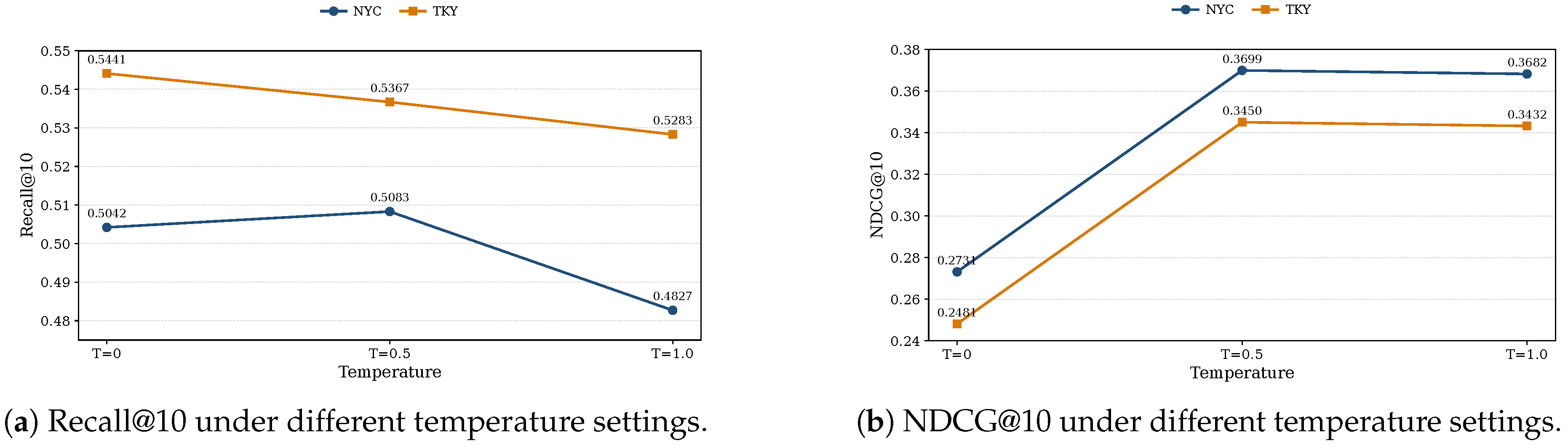
To study the effect of temperature scaling, we compare three settings (no temperature scaling, $T=0.5$, and $T=1.0$) and report Recall@10 and NDCG@10 in Figure 4. The temperature setting has a clear effect on both metrics, and the best performance is obtained when $T=0.5$. Once temperature scaling is introduced at the output layer, the model can better control the sharpness of the score distribution and improve recommendation quality. Without temperature scaling, the model tends to produce an overly sharp score distribution, which hurts ranking performance. We, therefore, use the results at $T=0.5$ as the final results.

5.6. Feature-Embedding-Dimension Study

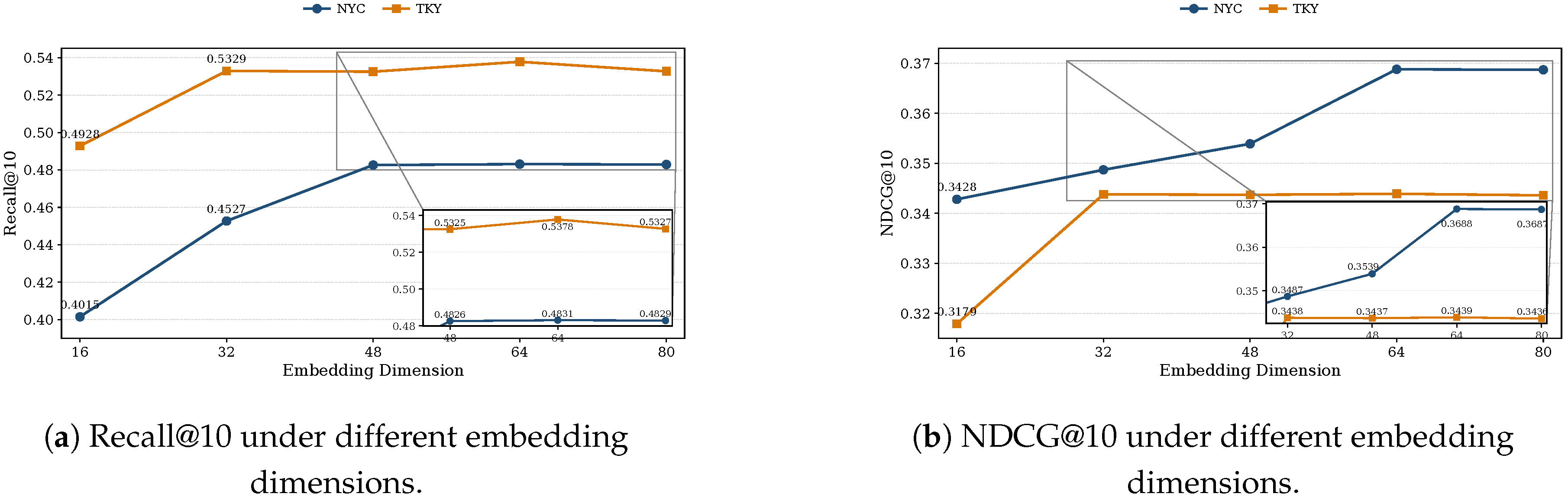
To study the effect of the feature-embedding dimension, we vary the dimension in $\{16,32,48,64,80\}$ and run experiments on both datasets. As shown in Figure 5, the best performance on both NYC and TKY is obtained when the embedding dimension is 64. More specifically, the performance of ASTHN first improves as the embedding dimension grows and then declines after a certain point. A dimension that is too small weakens representation capacity, while a dimension that is too large reduces generalization and may lead to overfitting.

5.7. Task Complexity Analysis

To analyze the efficiency and scalability of ASTHN, we report both theoretical time complexity and empirical running time. Let the trajectory length be L, the embedding dimension be d, and the GRU hidden dimension be H. For graph-based encoders, let k denote the sampled neighborhood size. For hypergraph aggregation, let $\left|\mathcal{E}\right|$ denote the number of hyperedges and let c denote the average number of incident nodes per hyperedge. For multi-head attention, let h denote the number of heads and let $d_h$ denote the dimension of each head. For diffusion-based models, let T denote the number of sampling steps, and let $|{\mathcal{E}}_g|$ denote the number of edges in the geographic graph.

Table 4. Theoretical time-complexity comparison of representative baselines and the proposed ASTHN.

Model	Time Complexity
STGN (RNN/LSTM-based)	$\mathcal{O}(L·d^2)$
STAN (Self-attention-based)	$\mathcal{O}(L^2·d)$
GETNext (Graph-based)	$\mathcal{O}(L·k·d·(k+d))$
STHGCN (Hypergraph + multi-head attention)	$\mathcal{O}\left(L·\left(h·\left|\mathcal{E}\right|·c·d_h+(|{\mathcal{V}}_q|+|{\mathcal{V}}_s|)·d_h^2\right)\right)$
Diff-POI (Diffusion/Generative)	$\mathcal{O}\left((|{\mathcal{E}}_g|+L^2+T)·d\right)$
ASTHN (Proposed)	$\mathcal{O}(M·K·|\mathcal{E}|·d+L·d·H)$

summarizes representative baselines from four common paradigms, including RNN-based sequence modeling (STGN), self-attention-based modeling (STAN), graph-based structure encoding (GETNext), hypergraph-based encoding with attention (STHGCN), and diffusion-based generative recommendation (Diff-POI).

RNN-based models such as STGN mainly rely on step-wise recurrent updates, so their dominant cost grows linearly with L and is commonly written as $\mathcal{O}(L·d^2)$. Self-attention-based models such as STAN require pairwise interaction among check-ins within a trajectory, which introduces an $\mathcal{O}(L^2)$ term and gives $\mathcal{O}(L^2·d)$. Graph-based methods such as GETNext further add neighborhood aggregation, so the cost grows with both L and neighborhood size k and can be summarized as $\mathcal{O}(L·k·d·(k+d))$ under neighbor sampling. Hypergraph models with attention such as STHGCN are more expensive because they involve both multi-head attention and hyperedge aggregation. If $|{\mathcal{V}}_q|$ and $|{\mathcal{V}}_s|$ denote the numbers of nodes in the query-side and support-side substructures used by the attention module, the total cost depends on h, $\left|\mathcal{E}\right|$, c, $|{\mathcal{V}}_q|$, and $|{\mathcal{V}}_s|$. Diffusion-based models such as Diff-POI add iterative sampling, which introduces an extra factor related to T beyond the encoder cost and is often summarized as $\mathcal{O}((|{\mathcal{E}}_g|+L^2+T)·d)$.

ASTHN contains two main components, multi-scale hypergraph aggregation and gated sequential modeling. The hypergraph component performs sparse aggregation on M hypergraph scales with K stacked HGNN layers, giving a dominant cost of $\mathcal{O}(M·K·|\mathcal{E}|·d)$. The sequence component uses a GRU to encode the fused-trajectory representation, giving a dominant cost of $\mathcal{O}(L·d·H)$. The overall time complexity of ASTHN is, therefore, $\mathcal{O}(M·K·|\mathcal{E}|·d+L·d·H)$. This form grows nearly linearly with structure size and trajectory length and avoids the quadratic dependence on L that often appears in attention-heavy models.

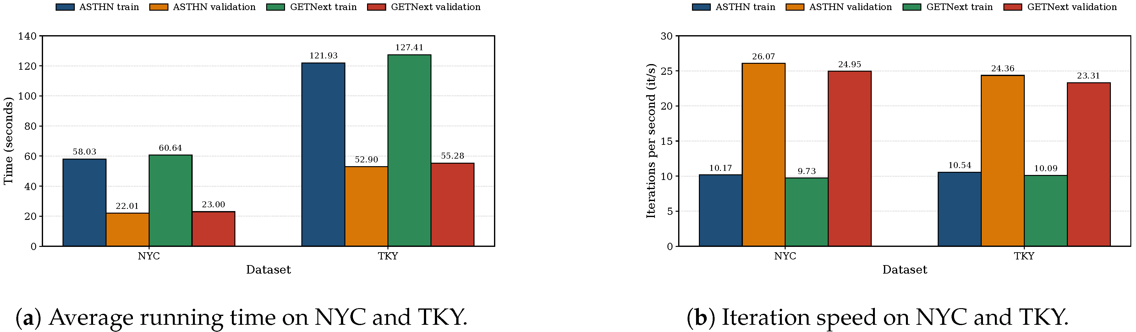
Beyond the theoretical analysis, we also conduct timing experiments on an NVIDIA GeForce RTX 3090 GPU with the NYC and TKY datasets, using GETNext as a representative competitor under the same training setting. Figure 6 reports the average running time and iteration speed. ASTHN achieves comparable or lower training cost than GETNext on both datasets, and its iteration speed remains stable across datasets. This is consistent with the near-linear complexity shown in Table 4 and suggests that ASTHN can scale to larger training sets while remaining practical to train.

5.8. Application-Scenario Visualization and Usability Analysis

To better reflect the potential use of ASTHN in urban-mobility services and personalized travel recommendations, this paper further conducts an application-oriented case analysis using held-out test queries. Each case is treated as an offline query-style recommendation scenario, where the current POI is regarded as the user’s current location, the ground-truth next POI is regarded as the actual next destination, and the model outputs a Top-K recommendation list. The analysis records the current POI, the ground-truth next POI, the Top-K recommended POIs, the hit result, and the rank of the ground-truth next POI.

To provide an interpretable spatial indicator, we compute the local POI supply density based on the POI coordinate table. For each POI, the number of POIs within a 1 km neighborhood is denoted as $n_{1\mathrm{km}}$, and the local POI supply density is defined as

$${\rho }_{1\mathrm{km}}=n_{1\mathrm{km}}/(\pi ·1^2)$$

(20)

with the unit approximately given as POIs/km². This metric describes the richness of POI supply around a location and is used only as an explanatory indicator for the case analysis. In addition, we calculate the average distance from the Top-10 recommended POIs to the current POI, denoted as MeanDist@10, and the average supply density of the Top-10 recommended POIs, denoted as MeanDensity@10, to quantify the spatial scale and regional characteristics of the recommendation results.

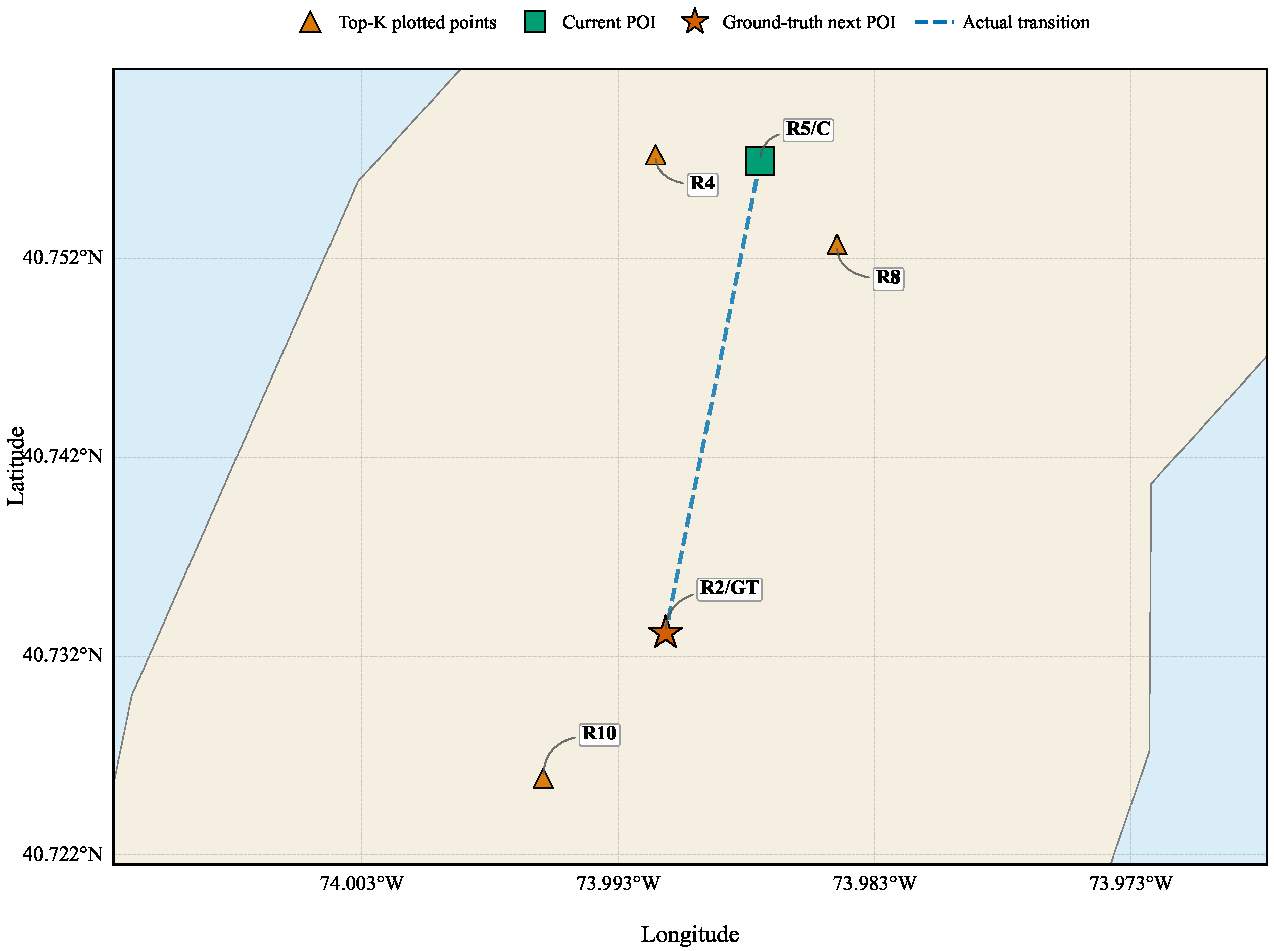
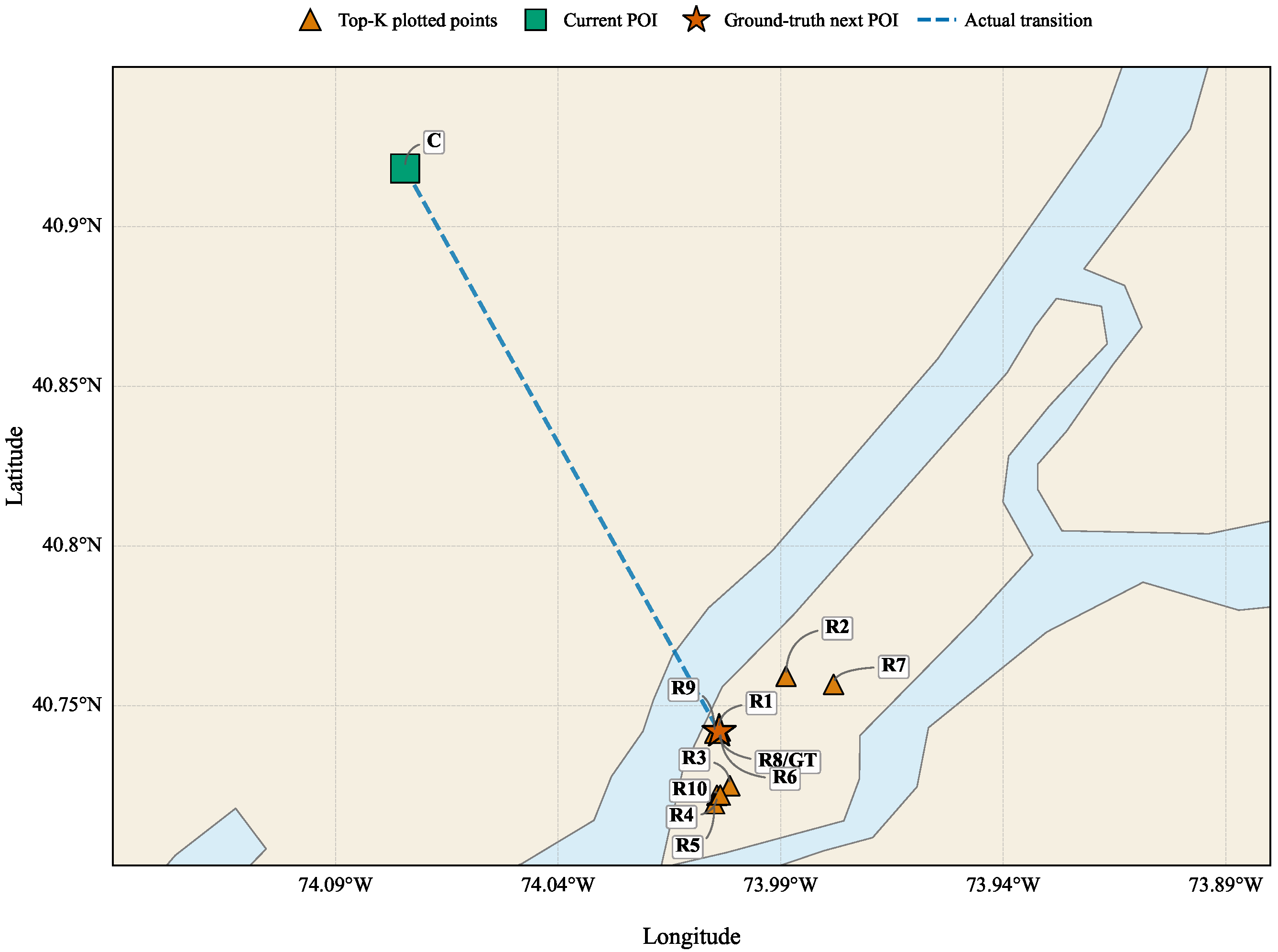
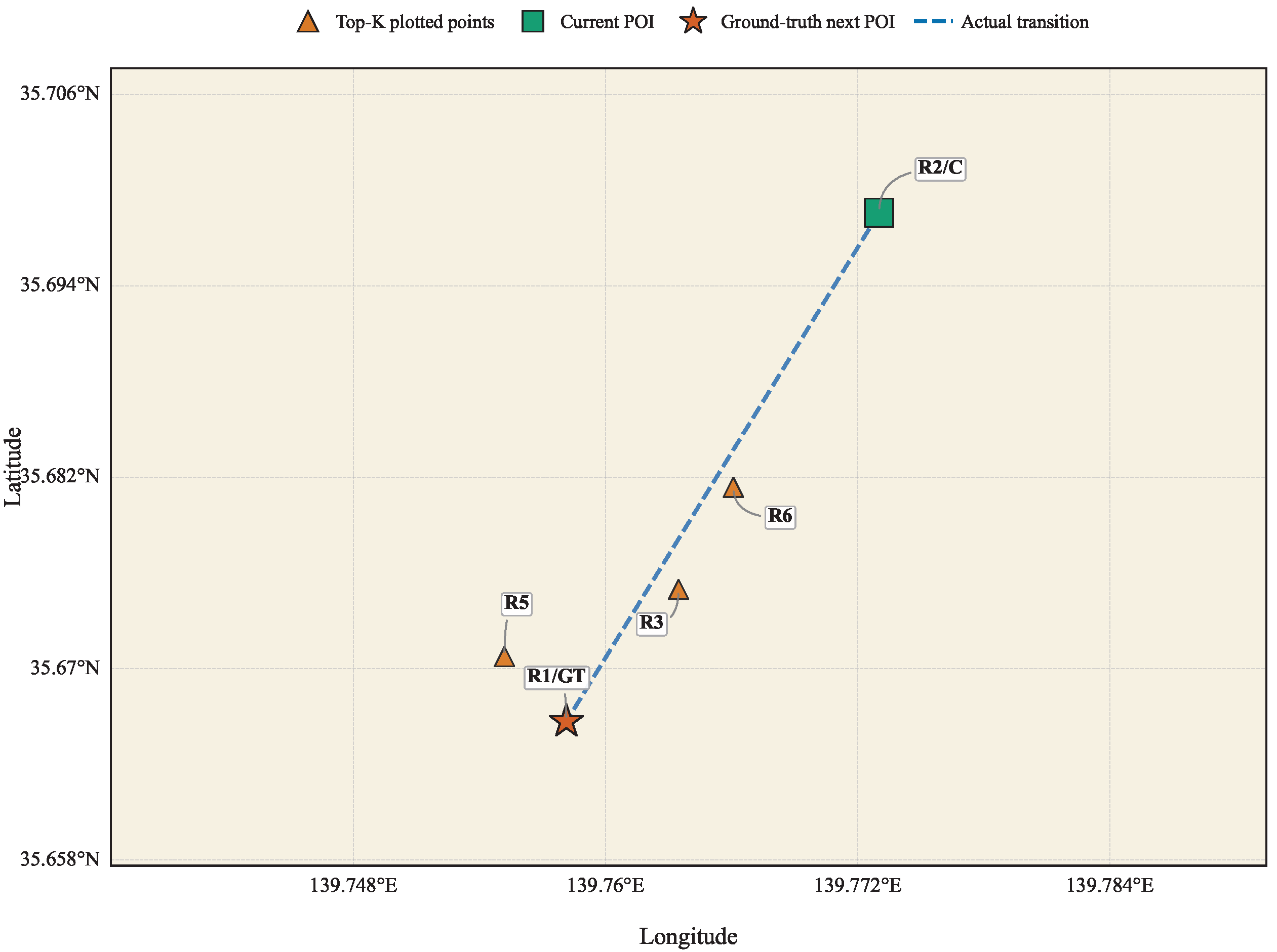
Figure 7, Figure 8 and Figure 9 present three representative cases, corresponding to long-distance migration, fine-grained ranking in a local high-density region, and a high-confidence hit during working hours. The figures use a unified notation: the green square denotes the current POI, the red star denotes the ground-truth next POI, the orange triangles denote the recommended POIs, and the blue dashed line connects the current POI and the ground-truth next POI to illustrate the actual migration scale. When dense candidate POIs cause label occlusion, the Top-10 recommended POIs are clustered according to spatial distance, and only representative points are retained for visualization. If a cluster contains the ground-truth next POI, the ground-truth point is retained with priority. Therefore, the visualized points represent the spatial distribution of the recommendation list, while MeanDist@10 and MeanDensity@10 are computed from the complete Top-10 results.

In the long-distance migration case NYC_test_167, shown in Figure 7, the straight-line distance between the current POI and the ground-truth next POI is approximately 20.48 km, indicating a cross-region migration scenario. ASTHN includes the ground-truth next POI in the Top-10 list, with the ground-truth POI ranked eighth, namely hit@10 = 1. The MeanDist@10 of this case is 21.11 km, which is close to the actual migration scale. This suggests that the recommendation list is not restricted to the local neighborhood of the current location. Meanwhile, the local supply density around the current POI is relatively low, with $n_{1\mathrm{km}}=158$ and ${\rho }_{1\mathrm{km}}\approx 50.29$, whereas the region of the ground-truth next POI has a higher supply density, with $n_{1\mathrm{km}}=1461$ and ${\rho }_{1\mathrm{km}}\approx 465.05$. The MeanDensity@10 further reaches 575.76. These results indicate that, in this query, ASTHN can cover a long-distance target region and the recommended POIs are associated with regions that have richer local POI supply.

In the local high-density ranking case NYC_test_137, shown in Figure 8, the current POI is located in a highly dense POI region, where the local density around the current point is ${\rho }_{1\mathrm{km}}\approx 902.09$, while the ground-truth next POI is approximately 2.66 km away. ASTHN ranks the ground-truth next POI second in the Top-K list, with hit@10 = 1. The MeanDist@10 is 3.80 km, and the MeanDensity@10 is 748.09. More importantly, although there are closer candidates in the Top-K list, such as candidates at 0.35 km and 0.53 km, the model still ranks the ground-truth next POI near the top. This case illustrates that the ranking is not dominated only by nearest-distance preference, and that ASTHN can distinguish fine-grained preferences among dense candidate POIs.

In the working-hour case TKY_test_1480, with hour = 9, as shown in Figure 9, ASTHN ranks the ground-truth next POI first, with hit@10 = 1 and rank = 1. In this case, the distance from the current POI to the ground-truth next POI is approximately 3.79 km, the MeanDist@10 is 3.91 km, and the MeanDensity@10 is 690.13. This result provides an example in which ASTHN gives a high-confidence hit during a specific time period. It also suggests that hourly preference can help the model distinguish candidate destinations at a similar spatial scale.

Overall, the above cases illustrate the practical usability of ASTHN from three complementary perspectives: cross-region migration coverage, fine-grained ranking under dense candidate regions, and time-sensitive recommendations during working hours. These observations are consistent with the three fine-grained spatio-temporal contexts explicitly modeled by ASTHN, namely minimum time intervals, spatial proximity, and hourly preferences. They provide intuitive evidence that ASTHN can support application scenarios such as personalized travel-destination recommendations.

6. Conclusions

This paper presents ASTHN, a next POI recommendation framework that combines fine-grained spatio-temporal context with hypergraph learning and adaptive fusion. ASTHN constructs three context hypergraphs from minimum time interval, geographic proximity, and hourly preference, and learns view-specific POI representations through hypergraph propagation. A two-stage fusion module aligns and adaptively integrates multi-view representations, while an ST-GRU with spatio-temporal gates captures trajectory dynamics. Temperature scaling is further applied at the output layer to mitigate overly concentrated score distributions.

Experiments on Foursquare-NYC and Foursquare-TKY demonstrate the effectiveness of ASTHN. The results in Table 3 show that ASTHN achieves the best performance on both datasets, with results reported as mean ± std over three random seeds. On NYC, ASTHN improves over the strongest baseline by 3.79% in Recall@5, 14.62% in Recall@10, 2.28% in NDCG@5, and 1.24% in NDCG@10. On TKY, the corresponding gains are 5.83%, 37.20%, 13.86%, and 20.49%. These results confirm the value of jointly modeling interval constraints, geographic reachability, and hourly periodicity. The application-oriented case visualizations further show that ASTHN can produce reasonable Top-K suggestions under different mobility patterns, including cross-region movement, dense local ranking, and time-sensitive commuting scenarios. The complexity analysis and timing results also indicate that ASTHN maintains competitive training cost and practical scalability.

ASTHN is designed for user-specific POI candidate sets in this study, and extending the framework to a larger candidate pool is a natural next step. Future work will also explore additional context signals when they are reliably available, and will further validate the method in scenario-driven urban-mobility and smart-tourism applications.

References

1. Li, Z.; Huang, X.; Liu, C.; Yang, W. Spatio-Temporal Unequal Interval Correlation-Aware Self-Attention Network for Next POI Recommendation. ISPRS Int. J. Geo-Inf. 2022, 11, 543. [Google Scholar] [CrossRef]
2. Tian, J.; Zhao, Z.; Ding, Z. Next Point-of-Interest Recommendation Based on Joint Mining of Spatial-Temporal and Semantic Sequential Patterns. ISPRS Int. J. Geo-Inf. 2023, 12, 297. [Google Scholar] [CrossRef]
3. Koren, Y.; Bell, R.; Volinsky, C. Matrix Factorization Techniques for Recommender Systems. Computer 2009, 42, 30–37. [Google Scholar] [CrossRef]
4. Rendle, S.; Freudenthaler, C.; Schmidt-Thieme, L. Factorizing Personalized Markov Chains for Next-Basket Recommendation. In Proceedings of the 19th International Conference on World Wide Web (WWW), Raleigh, NC, USA, 26–30 April 2010; pp. 811–820. [Google Scholar] [CrossRef]
5. Liu, Q.; Wu, S.; Wang, L.; Tan, T. Predicting the Next Location: A Recurrent Model with Spatial and Temporal Contexts. In Proceedings of the AAAI Conference on Artificial Intelligence, Phoenix, AZ, USA, 12–17 February 2016; Volume 30. [Google Scholar] [CrossRef]
6. Luo, Y.; Liu, Q.; Liu, Z. STAN: Spatio-Temporal Attention Network for Next Location Recommendation. In Proceedings of the Web Conference (WWW), Ljubljana, Slovenia, 19–23 April 2021; pp. 2177–2185. [Google Scholar] [CrossRef]
7. Xu, S.; Huang, Q.; Zou, Z. Spatio-Temporal Transformer Recommender: Next Location Recommendation. ISPRS Int. J. Geo-Inf. 2023, 12, 79. [Google Scholar] [CrossRef]
8. Yang, S.; Liu, J.; Zhao, K. GETNext: Trajectory Flow Map Enhanced Transformer for Next POI Recommendation. arXiv 2023, arXiv:2303.04741. [Google Scholar] [CrossRef]
9. Qin, Y.; Wang, Y.; Sun, F.; Ju, W.; Hou, X.; Wang, Z.; Cheng, J.; Lei, J.; Zhang, M. DisenPOI: Disentangling Sequential and Geographical Influence for Point-of-Interest Recommendation. In Proceedings of the Sixteenth ACM International Conference on Web Search and Data Mining (WSDM), Singapore, 27 February–3 March 2023; pp. 508–516. [Google Scholar] [CrossRef]
10. Zuo, C.; Zhang, X.; Yan, L.; Zhang, Z. GUGEN: Global User Graph Enhanced Network for Next POI Recommendation. IEEE Trans. Mob. Comput. 2024, 23, 14975–14986. [Google Scholar] [CrossRef]
11. Yan, X.; Song, T.; Jiao, Y.; He, J.; Wang, J.; Li, R.; Chu, W. Spatio-Temporal Hypergraph Learning for Next POI Recommendation. In Proceedings of the 46th International ACM SIGIR Conference on Research and Development in Information Retrieval (SIGIR), Taipei, China, 23–27 July 2023; pp. 403–412. [Google Scholar] [CrossRef]
12. Wang, H.; Li, P.; Liu, Y.; Shao, J. Towards Real-Time Demand-Aware Sequential POI Recommendation. Inf. Sci. 2021, 547, 482–497. [Google Scholar] [CrossRef]
13. Yu, J.; Guo, L.; Zhang, J.; Wang, G. A Survey on Graph Neural Network-Based Next POI Recommendation for Smart Cities. J. Reliab. Intell. Environ. 2024, 10, 299–318. [Google Scholar] [CrossRef]
14. Feng, S.; Cong, G.; An, B.; Chee, Y.M. Personalized Ranking Metric Embedding for Next New POI Recommendation. In Proceedings of the 24th International Conference on Artificial Intelligence (IJCAI), Buenos Aires, Argentina, 25–31 July 2015; pp. 2069–2075. [Google Scholar]
15. Sun, K.; Qian, T.; Chen, T.; Liang, Y.; Nguyen, Q.V.H.; Yin, H. Where to Go Next: Modeling Long- and Short-Term User Preferences for Point-of-Interest Recommendation. In Proceedings of the AAAI Conference on Artificial Intelligence, New York, NY, USA, 7–12 February 2020; Volume 34, pp. 214–221. [Google Scholar] [CrossRef]
16. Zhao, P.; Zhu, H.; Liu, Y.; Xu, J.; Zhou, K.; Sheng, V.S. STGN: Spatio-Temporal Gated Network for Point-of-Interest Recommendation. In Proceedings of the AAAI Conference on Artificial Intelligence, Honolulu, HI, USA, 27 January–1 February 2019. [Google Scholar]
17. Wu, Y.; Li, K.; Zhao, G.; Qian, X. Personalized Long- and Short-term Preference Learning for Next POI Recommendation. IEEE Trans. Knowl. Data Eng. 2022, 34, 1944–1957. [Google Scholar] [CrossRef]
18. Fang, J.; Meng, X. URPI-GRU: An Approach of Next POI Recommendation Based on User Relationship and Preference Information. Knowl.-Based Syst. 2022, 256, 109848. [Google Scholar] [CrossRef]
19. Wang, D.; Wan, F.; Yu, D.; Shen, Y.; Xiang, Z.; Xu, Y. Context- and Category-Aware Double Self-Attention Model for Next POI Recommendation. Appl. Intell. 2023, 53, 18355–18380. [Google Scholar] [CrossRef]
20. Wu, J.; Jiang, S.; Shi, L. A Next POI Recommendation Based on Graph Convolutional Network by Adaptive Time Patterns. Electronics 2023, 12, 1241. [Google Scholar] [CrossRef]
21. Wang, Z.; Zhu, Y.; Liu, H.; Wang, C. Learning Graph-Based Disentangled Representations for Next POI Recommendation. In Proceedings of the 45th International ACM SIGIR Conference on Research and Development in Information Retrieval (SIGIR), Madrid, Spain, 11–15 July 2022; pp. 1154–1163. [Google Scholar] [CrossRef]
22. Wang, Z.; Zhu, Y.; Zhang, Q.; Liu, H.; Wang, C.; Liu, T. Graph-Enhanced Spatial-Temporal Network for Next POI Recommendation. ACM Trans. Knowl. Discov. Data 2022, 16, 1–21. [Google Scholar] [CrossRef]
23. Lai, Y.; Su, Y.; Wei, L.; He, T.; Wang, H.; Chen, G.; Zha, D.; Liu, Q.; Wang, X. Disentangled Contrastive Hypergraph Learning for Next POI Recommendation. In Proceedings of the 47th International ACM SIGIR Conference on Research and Development in Information Retrieval (SIGIR), Washington, DC, USA, 14–18 July 2024. [Google Scholar] [CrossRef]
24. Lai, Y.; Su, Y.; Wei, L.; Chen, G.; Wang, T.; Zha, D. Multi-view Spatial-Temporal Enhanced Hypergraph Network for Next POI Recommendation. In Database Systems for Advanced Applications, 28th International Conference, DASFAA 2023, Tianjin, China, 17–20 April 2023, Proceedings, Part II; Lecture Notes in Computer Science; Springer: Berlin/Heidelberg, Germany, 2023. [Google Scholar] [CrossRef]
25. An, J.; Gao, M.; Tang, J. MvStHgL: Multi-View Hypergraph Learning with Spatial-Temporal Periodic Interests for Next POI Recommendation. ACM Trans. Inf. Syst. 2024, 42, 1–29. [Google Scholar] [CrossRef]
26. Duan, J.; Meng, X.; Liu, G. Where To Go at the Next Timestamp. Data Sci. Eng. 2024, 9, 88–101. [Google Scholar] [CrossRef]
27. Xu, Y.; Shen, H.; Jiang, Y.; Wang, E. Where and When: Predict Next POI and Its Explicit Timestamp in Sequential Recommendation. In Proceedings of the Thirty-Fourth International Joint Conference on Artificial Intelligence (IJCAI), Montreal, QC, Canada, 16–22 August 2025. [Google Scholar] [CrossRef]
28. Zhang, X.; Liu, D.; Yan, L.; Zhang, Z.; Li, Y. Graph-Enhanced Spatio-Temporal Interval Aware Network for Next POI Recommendation in Mobile Environment. J. Internet Technol. 2024, 25, 619–628. [Google Scholar] [CrossRef]
29. He, X.; He, W.; Liu, Y.; Lu, X.; Xiao, Y.; Liu, Y. ImNext: Irregular Interval Attention and Multi-Task Learning for Next POI Recommendation. Knowl.-Based Syst. 2024, 293, 111674. [Google Scholar] [CrossRef]
30. Zhou, Y.; Zhang, D.; Zhou, K.; Han, P. Context-Aware Knowledge Graph Learning for Point-of-Interest Recommendation. ISPRS Int. J. Geo-Inf. 2026, 15, 14. [Google Scholar] [CrossRef]
Figure 1. Illustrative example of a user check-in sequence and its spatio-temporal patterns.
Ijgi 15 00242 g001
Figure 2. Overall architecture of ASTHN.
Ijgi 15 00242 g002
Figure 3. Ablation study of ASTHN on the NYC and TKY datasets. Panel (a) shows Recall@10, and panel (b) shows NDCG@10. The results indicate that both the time-interval branch and the hourly-preference branch contribute substantially to overall performance.
Ijgi 15 00242 g003
Figure 4. Effect of the temperature parameter on ASTHN. Panel (a) shows Recall@10, and panel (b) shows NDCG@10 under different settings of T. The best overall performance is obtained when T = 0.5 , which indicates that appropriate temperature scaling improves score calibration and ranking quality.
Ijgi 15 00242 g004
Figure 5. Effect of the feature-embedding dimension on ASTHN. Panel (a) presents Recall@10, and panel (b) presents NDCG@10. The model achieves the best trade-off between representation capacity and generalization when the embedding dimension is set to 64.
Ijgi 15 00242 g005
Figure 6. Running-efficiency comparison of ASTHN. Panel (a) reports the average running time, and panel (b) reports the iteration speed. The results indicate that ASTHN maintains competitive computational cost while preserving strong representation capability on both datasets.
Ijgi 15 00242 g006
Figure 7. NYC_test_167: long-distance migration case with a Top-10 hit and rank = 8. The green square denotes the current POI, the red star denotes the ground-truth next POI, the orange triangles denote recommended POIs, and the blue dashed line shows the straight-line connection between the current POI and the ground-truth next POI.
Ijgi 15 00242 g007
Figure 8. NYC_test_137: fine-grained ranking case in a local high-density region with a Top-10 hit and rank = 2. The recommended points are clustered for visualization to reduce label occlusion in the dense local region.
Ijgi 15 00242 g008
Figure 9. TKY_test_1480: working-hour case with hour = 9, a Top-1 hit, and rank = 1. This case illustrates the model’s time-sensitive recommendation behavior during a specific daily period.
Ijgi 15 00242 g009