MDSR-KG: A Geographical Knowledge Graph Framework for Representing and Quantifying Spatial Relationships

Abstract

Geographical knowledge graphs (GeoKGs) have long experienced several fundamental challenges in representing complex spatial relationships, such as limited dimensionality, insufficient quantification of relationship strength, and weak reasoning capabilities. To address these issues, this study presents the multidimensional spatial relation knowledge graph (MDSR-KG) framework. The novelty of this framework lies in advancing the shift toward spatial relation node-based representation, thereby elevating the spatial relations from edge structures to independent, computable, and inferable structured nodes. This approach was complemented by a parametric method aimed at quantifying the relation strength between nodes, thereby facilitating an advancement from discrete relations to continuous and interpretable association weighting. In experiments conducted in this study using the Berlin OpenStreetMap data, we noted that for complex spatial queries, the MDSR-KG framework significantly outperformed the baseline models in accuracy and completeness. The framework also exhibited advanced reasoning capabilities, such as ranking and recommendation, which are lacking in traditional methods. Thus, the framework lays a theoretical foundation for advancing from geographic feature recognition to spatial relationship comprehension.

1. Introduction

Geographic knowledge graphs (GeoKGs) integrate geographic information with knowledge graph technologies, providing a structured knowledge representation framework for geographic entities, concepts, and their interrelationships [1]. In recent years, GeoKGs have demonstrated significant potential in fields such as remote sensing image interpretation, natural disaster monitoring, and land cover mapping, emerging as a research hotspot in geographic information science [2,3,4,5]. GeoKGs are crucial methods to acquire geographic knowledge and understand the geographic environment [6], covering the dual representation of geographic entities and spatial relationships. Spatial relationships encompass the distribution, arrangement, and interrelations of geographic entities. Accurately representing spatial relationships is essential to intelligent geographic analysis and solving real-world geographic challenges [7,8]. With the United Nations Sustainable Development Goal (SDG) 11.3 emphasizing smart city management, demand for precise spatial relationship analysis has increased [9]

Representation of spatial relationships is the focus of this paper, which refers to the comprehensive description of spatial associations between geographic entities from three dimensions: topology, metrics, and semantics [10]. Topology captures intuitive concepts of human visual perception, describing logical connections and containment between entities (e.g., “contains,” “adjacent”). Metrics refer to quantitative geometric characteristics (e.g., Euclidean distance). Semantics describe functional or scene associations in the form of predicates (e.g., “provides water source for”). These three dimensions complement each other, jointly forming a complete description of spatial relationships.

Knowledge graphs can represent and analyze geographic knowledge’s unique spatial characteristics and relationships in a semantic and structured form [11,12,13,14]. However, existing geographic knowledge graphs suffer from three fundamental limitations in representing spatial relationships. First, spatial relationship representations lack multidimensionality. They fail to integrate comprehensive information from topology, metrics, and semantics, thus failing to capture complex interaction patterns across target regions. Existing knowledge graphs primarily focus on either topological or high-level semantic relationships, without systematically integrating multidimensional spatial features [15,16]. Second, methods for quantifying relationship strength are inadequate. Relationships are typically represented as binary values, with few studies employing static empirical weights [17,18]. The absence of continuous metrics limits reasoning in complex scenarios. For example, answering a query such as “find commercial areas that are close to a main road (<150 m) and far from residential areas (>300 m)” requires the system to simultaneously handle multiple spatial constraints and quantify their trade-offs, which existing GeoKGs can hardly support. It is worth noting that although traditional spatial databases can compute geometric quantities such as distance and area in real time, such outputs are single-dimensional raw values (e.g., “150 m”) and cannot directly reflect the integrated relationship strength that combines topology, area, and semantics. In real-world tasks such as geographic cognition and complex reasoning (e.g., influence ranking, suitability recommendation), humans typically need to integrate multidimensional information from topology, metrics, and semantics. The quantification model is designed precisely to fill this gap. Third, integration between representation models and reasoning capabilities remains insufficient. Existing knowledge graph frameworks exhibit weaknesses in complex spatial queries and reasoning. Notably, Simplified representations of spatial relationships limit their support for advanced applications such as path planning, scene analysis, and spatial decision-making.

To address these issues, this study proposes a multidimensional spatial relation knowledge graph (MDSR-KG) representation framework. The main contributions are:

• Core structural innovation: The framework uses the spatial relationship node-based representation tuple approach, elevating spatial relationships from simple edge structures to independent nodes that are rich in attributes. This provides a structured container for multidimensional relationship descriptions, thereby solving the problem of structured expression for complex spatial relationships.
• Core quantitative innovation: It adopts a parameterized relationship strength quantification method that integrates multiple dimensions of spatial relationships of geographic entities. This approach extends from establishing traditional binary relationships to ensuring continuous strength measurements. offering a quantitative foundation for analyzing the interactions between the geographic features in a geographic scenario.
• Engineering enabler: The framework offers an end-to-end automated graph construction workflow, delivering a practical solution for efficiently converting raw geographic data into inferable knowledge graphs.

The innovative knowledge graph representation framework proposed in this study aims to systematically address the core challenges in spatial relationship representation and quantification within geographic knowledge graphs, thereby filling a theoretical gap in modeling complex spatial relationships.

2. Related Literature

The representation of geospatial information by machines was initially realized using traditional spatial database systems [19]. However, there are fundamental differences between the database systems and knowledge graphs. Traditional spatial databases (e.g., PostGIS, Oracle Spatial) are relational databases that focus on data storage and retrieval, as well as efficient geometric computation. They treat spatial relations merely as computational outputs (e.g., distance values) rather than as independently addressable, property-accumulable knowledge units [20]. Consequently, they struggle to support geospatial relational reasoning and semantic analysis. In contrast, knowledge graphs explicitly represent semantic relations between entities through a graph structure, placing greater emphasis on knowledge semantics, relational reasoning, and contextual understanding. Each approach has its own strengths. This paper focuses on the representation of geospatial relations—an area where knowledge graphs naturally excel.

Geographic knowledge graphs [1], integrating geographic information systems (GIS) with artificial intelligence (AI) technologies, are an emerging and significant research direction in geoinformation science. Their development trajectory clearly shows an evolution “from general to domain-specific, and from semantic to geometric”.

Early general knowledge graphs were mostly semantic-driven. Geographic knowledge graphs mainly represent concepts, entities, and semantic relationships in geographic science. Constructed via semantic extraction from sources like text, encyclopedias, and databases, they emphasize names, attributes, and semantic relationships of geographic entities, with limited use of spatial coordinates or geometric features. Graphs like YAGO [21] and DBpedia [22] cover broad domains (persons, places, organizations, events) and include geographic information such as coordinates and latitude-longitude for entities like countries, cities, and landmarks [23]. Advancements in natural language processing (NLP) enable automatic extraction of complex semantic relationships from text [24,25], expanding spatial representation (e.g., “disaster impact region” [26,27,28]). Though effective for semantic connections [29], these approaches often neglect the geometric and topological properties, thereby limiting applications in geographic scenarios.

As knowledge graphs have developed in specialized domains, research emphasized that the geographic knowledge graphs require richer spatial data representation [30] to better capture complex spatial relationships among entities [31,32]. Geographic knowledge graphs began to focus on geometric characteristics, incorporating spatial data details like coordinates, boundaries, shapes, and topological relationships. For example, graphs such as LinkedGeoData [33], CrowdGeoKG [34], and WorldKG [35] represent geographic entities in RDF format, achieving a preliminary integration of geometric and semantic information. The advantage of these knowledge graphs lies in their scale and coverage, but their spatial relations are mainly inherited from the native attributes of the data sources, lacking a formalized enhancement of the relations themselves. Subsequently, knowledge graphs based on geographic theory have been proposed. The formal Geographic Knowledge Graph(GeoKG) framework [36] employs a six-element structure and extended attributive language and complements (ALC) description logic to represent the states, evolutions, and mechanisms of geographic entities. Geographic evolution knowledge graph (GEKG) is a hierarchical cube model for representing geographic evolutionary knowledge, encompassing core elements (e.g., time, events, geographic entities, activities, and attributes). This structure forms a time-hierarchical framework, establishing complex interconnections between different temporal layers [11]. Augmented geographic knowledge graph (AugGKG) is a grid-enhanced geographic knowledge graph designed for spatiotemporal data. Owing to its grid-based design and hidden layers, it can significantly improves the efficiency of spatiotemporal queries [37]. The Hierarchical Geographic Knowledge Graph (HGeoKG) can extend spatial relationship representation from simple topology to complex spatial semantics, constructing the spatial relationships of geographic entities based on the Dimensionally Extended Nine-Intersection Model (DE-9IM) [38]. These studies provide formal definitions for geographic space and enhanced geometric expression [39,40].

In terms of spatial representation methods, while professional geographic knowledge graphs incorporate spatial dimensions, the majority of existing approaches provide only the basic geospatial information, with limited capabilities for integrating and expressing multidimensional relationships [41,42]. In summary, neither traditional spatial databases nor existing GeoKGs can address the three fundamental limitations identified in the introduction: single-dimensional representation, lack of relationship strength quantification, and weak reasoning capability.

3. Methodology

3.1. Framework

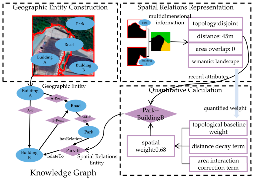
This study proposes the MDSR-KG framework to address key challenges in geographic knowledge graphs: single-dimensional spatial relationship representation, inadequate quantification methods, and insufficient reasoning capabilities. As illustrated in Figure 1, the framework establishes a systematic multidimensional spatial relationship representation system, marking a shift from traditional edge-based to node-based relationship representation.

The primary objective is to effectively express spatial distributions and associations of geographic entities in real-world scenarios. At its core, the framework elevates spatial relations from subordinate edge attributes to independent nodes, establishing the foundational “geographic entity–spatial relation–geographic entity” triplet. Furthermore, it incorporates quantitative analysis of geographic spatial relationship strength to overcome the limitations of conventional knowledge graphs in representing complex spatial relationships.

The MDSR-KG framework encompassed three main modules:

• Entity construction module: The module was based on geographic entity nodes [11,36], representing the objects in the scene (e.g., buildings, roads, and rivers). Each entity node integrated the semantic, geometric, and attribute information of the geographical object. Typically, the relevant information was extracted from RS data (such as satellite imagery and vector data) to generate the nodes.
• Relationship representation module: The core of this module was the spatial relationship nodes, representing the spatial relationships between geographic objects (e.g., the spatial relationship between a lake and a park). The spatial relationships in the module were represented as independent entity nodes. The spatial relationship nodes integrated multidimensional geographic entity association information, including topology, metrics, and semantics.
• Quantitative calculation module: Based on the representation nodes for geographic entities and spatial relationships, it constructed a parameterized weight quantification algorithm for object associations within the scene by integrating multidimensional information of spatial relationships. The quantified weights measured the degree of mutual influence between geographical entities, thereby enhancing the knowledge graph’s reasoning capabilities for complex spatial relationships.

The core innovation of MDSR-KG lies in the integration of relation node-based representation (Section 3.3) and relationship strength quantification (Section 3.4), which together transform discrete spatial relations into computable, comparable, and inferable knowledge units.

3.2. Core Components

The MDSR-KG framework produced a comprehensive geospatial knowledge representation around four core elements:

• Geographic entities: Geographic entities are independent objects in a real geographic environment, e.g., buildings, roads, water, and vegetation areas. Each entity is represented as an independent node in the knowledge graph, serving as the fundamental unit for spatial relationship analysis.
• Geographic entity attributes: Geographic entities can be comprehensively described through multiple types of attributes, including semantic, geometric, and spatial properties. Semantic attributes primarily include information, such as object type, functional classification, and name identifiers. Geometric attributes refer to measurable characteristics, such as the geometric shape, area, perimeter, and spatial extent of a geographic entity. Spatial attributes include location coordinates, boundary range, and bounding box.
• Spatial relationships: As the core innovation of the framework, spatial relationships are represented as independent nodes that define the spatial associations between geographic entities. This mode of representation breaks the limitations of traditional edge structures, providing a structured container for describing multidimensional relationships.
• Spatial relationship attributes: Spatial relationship nodes are described in detail through multidimensional attributes (e.g., topology, metric, and semantics). Topological attributes are based on the Open Geospatial Consortium’s (OGC) standard [43] for spatial connectivity logic (e.g., intersect, contain, and adjacent). Metric attributes describe the quantitative characteristics of spatial relationships (such as distance, orientation, and overlapping area). Semantic attributes refer to the functional associations and directional relationships between geographic entities.

3.3. Multidimensional Spatial Relationship Representation

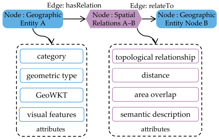
In the MDSR-KG framework, the “entity construction module” represents a mature method for depicting the geographic entities in knowledge graphs [11,36], providing a solid foundation for the model. The “relationship representation module” is the core innovation of the model, elevating the spatial relationships from the edge attributes attached to entities to the independent nodes. The nodes are on par with geographic entities and enriched with multidimensional attributes [44]. The integration of spatial relationships with geographic entities generates a more expressive representation tuple of “Entity-Relationship-Entity”, as shown in Figure 2. This tuple structure reifies spatial relations as first-class nodes, enabling them to carry attributes, be directly queried, and support advanced reasoning—a theoretical shift from edge-based representations.

3.3.1. Model Definition

The graph structure of the MDSR-KG model can be mathematically expressed as follows:

$$G=\left(V,E\right),V=\left\{v\right\},E=\left\{edge\right\},$$

(1)

where V denotes the node set, comprising two node types: geographic entity and spatial relation. E denotes the edge set that describes the connections between the nodes.

Definition 1.

Geographic Entity,

The set of geographic entity, $V_{entity}$ can be defined as follows:

$$V_{entity}={\left\{v_i^e\right\}}_{i=1}^n$$

(2)

where each entity, $v_i^e$, represents a geographic object with the following attributes:

$$A_{entity}=\left\{C,S,W,F\right\}$$

(3)

where C denotes the category of geographic object (e.g., road and building), and S denotes the geometric type (e.g., point, line, and polygon). W denotes the geometric information, which employs the well-known text (WKT) format to record in a compact and human-readable manner. F denotes the visual features, which can be extracted from Remote Sensing data to capture the entity’s characteristics in imagery for future study.

Definition 2.

Spatial Relations,

The spatial relation set $V_{spatio}$ can be defined as follows:

$$V_{spatio}={\left\{v_{ij}^s\right\}}_{i,j=1}^n$$

(4)

Each spatial relationship set, $v_{ij}^e$, represents the spatial association between geographic objects $v_i^e$ and $v_j^e$ with the following attributes:

$$A_{spatio}=\left\{T,d_{ij},{\rho }_{ij},Sem\right\}$$

(5)

These attributes capture both discrete and continuous spatial relations. Discrete relations (e.g., topological relationship, semantic connectivity) are stored in T and Sem. Continuous metrics provide distance and overlap measures. The two coexist within each relation node, supporting both categorical queries and quantitative analysis.

The T denotes the topological relationship between the geographic objects, with $T\in P_{topo}$. The $P_{topo}$ is a set of topological relationship predicates defined based on the OGC standard [44,45].

$$P_{topo}=\left\{\mathrm{e}\mathrm{q}\mathrm{u}\mathrm{a}\mathrm{l}\mathrm{s},\mathrm{c}\mathrm{o}\mathrm{n}\mathrm{t}\mathrm{a}\mathrm{i}\mathrm{n}\mathrm{s},\mathrm{w}\mathrm{i}\mathrm{t}\mathrm{h}\mathrm{i}\mathrm{n},\mathrm{o}\mathrm{v}\mathrm{e}\mathrm{r}\mathrm{l}\mathrm{a}\mathrm{p}\mathrm{s},\mathrm{c}\mathrm{r}\mathrm{o}\mathrm{s}\mathrm{s}\mathrm{e}\mathrm{s},\mathrm{t}\mathrm{o}\mathrm{u}\mathrm{c}\mathrm{h}\mathrm{e}\mathrm{s},\mathrm{d}\mathrm{i}\mathrm{s}\mathrm{j}\mathrm{o}\mathrm{i}\mathrm{n}\mathrm{t}\right\}$$

(6)

Note that to simplify the model, the OGC standard relation covers and coveredBy are respectively subsumed under contains and within. Additionally, intersects—as a generalization of the above relations (except disjoint)—was not listed as a base predicate in the model. Instead, it was logically inferred through the union of other relations.

The distance between entities, $d_{ij}$, represented the geometric distance metric between the geographic objects. In accordance with Tobler’s First Law of Geography, the relative distance is crucial for understanding spatial relationships. $d_{ij}$ was calculated using the following formula:

$$d_{ij}=dist\left(v_i^e,v_j^e\right)={min}_{p\in v_i^e,q\in v_j^e}‖p-q‖$$

(7)

where $dist\left(v_i^e,v_j^e\right)$ denotes the minimum Euclidean distance between geographic objects, directly reflecting true proximity in geographic space.

Area overlap, ${\rho }_{ij}$, is the area interaction metric between the geographic objects, reflecting the spatial interaction intensity. ${\rho }_{ij}$ was calculated using the following formula:

$${\rho }_{ij}={\displaystyle \frac{area\left(v_i^e\cap v_j^e\right)}{avg\left(area\left(v_i^e\right),area\left(v_j^e\right)\right)}}$$

(8)

where $area\left(v^e\right)$ represents the area of geographic object $v^e$, while avg denotes the average of the areas of the geographic objects.

Sem denotes the semantic description, represented using predefined vocabulary to denote the functional roles, such as “landscape water” and “irrigation water sources.” Semantic descriptions are assigned via a semi-automatic pipeline: basic labels are extracted from OpenStreetMap(OSM) tags (e.g., fclass, name) and mapped to a geographic ontology; relation-specific semantics (e.g., “provides ecological service”) are inferred by rules combining topological predicates and entity types.

Definition 3.

Tuple,

Complete geospatial relationships can be expressed through structured tuples “Entity-Relationship-Entity”, as shown below:

$$Tuple\left(v_i^e,v_j^e\right)=\left(v_i^e,edge,v_{ij}^s,edge,v_j^e\right)=\left\{v_i^e\stackrel{hasRelation}{\to }{v}_{ij}^s\stackrel{relateTo}{\to }{v}_j^e\right\}$$

(9)

where $Tuple\left(v_i^e,v_j^e\right)$ indicates the existence of a spatial relation $v_{ij}^s$ between $v_i^e$ and $v_j^e$.

The model connects geographic entities and their spatial relationships using the set of $edge\in E$. The edges include two types of directed connections. The first is hasRelation, which points from a geographic entity to a spatial relation node, indicating that the starting geographic entity $v_i^e$ has a spatial relationship $v_{ij}^s$ with another geographic entity. The second is relateTo, which points from a spatial relation node to a geographic entity, indicating the target geographic entity $v_j^e$ associated with the spatial relationship $v_{ij}^s$. The edge directionality encodes the “subject-relation-object” semantics: hasRelation links the subject entity to the relation node, and relateTo links the relation node to the object entity. These edges carry no additional attributes and serve only as structural links for graph traversal. As shown in formula 9, entities and edges form a tuple. The tuple is the minimal unit for representing geospatial relationships in knowledge graphs. This helps the model to achieve an advancement from simple connections to rich descriptions.

3.3.2. Theoretical Analysis

Existing spatial relation modeling approaches are typically constrained to single-dimensional representation (e.g., DE-9IM’s focus on topology or Web Ontology Language’s (OWL) on semantics). Traditional geographic knowledge graphs predominantly represent spatial relations as simple “edges” that connect geographic entity nodes, which primarily record the existence of a relationship while carrying limited flat attributes. This conventional “edge” structure is essentially an attribute appendage, leading to two principal limitations: its singular expressive dimension struggles to accommodate heterogeneous spatial information, and the non-computable structure constrains complex spatial analysis.

The core innovation of the MDSR-KG drives a shift from “edge attributes” to “nodes.” By elevating spatial relationships to independent entities enriched with multiple dimensions, the model resolves the fundamental flaws of traditional structures. The nodalization of spatial relations provides a structured schema for describing complex geospatial relationships and enables spatial relationships to be treated as direct objects in computational contexts. The spatial relationships to become addressable and traversable entities within the knowledge graph (e.g., “find all relationships with strength > τ”) [46,47]. This substantially enhances the declarative querying capabilities of knowledge graphs.

As independent nodes, spatial relationships can possess multidimensional attribute sets, systematically organized within a structured schema. This structure integrates topological predicates, metric measures, and semantic information. This moves beyond the single-dimensional focus of existing methods, providing a structural foundation for complex, fine-grained descriptions.

Furthermore, the structured representation in the MDSR-KG model elevates knowledge graph reasoning capabilities. Independent spatial relation nodes serve as the natural units for graph computation and reasoning. Advanced reasoning algorithms can be designed based on the multidimensional attributes of spatial relation nodes, such as quantitative computation of relation strength and semantic analysis of relation paths. This approach transforms spatial relations from static records into dynamic computational units, marking a substantial advancement from mere association identification to deeper relation understanding.

3.4. Spatial Relationship Quantification

The “quantitative calculation module” of the MDSR-KG framework transforms geographic entity association information into computable and comparable numerical forms through mathematical methods, enabling the precise quantification of the spatial relationship strengths between the geographic entities. Quantification is essential because raw geometric measures (e.g., distance, area) are insufficient for tasks requiring integrated assessment of spatial influence, such as ranking and multi-constraint recommendation. MDSR-KG addresses this by producing a unified strength value that combines topology, area interaction, and distance decay.

3.4.1. Spatial Weight Matrix

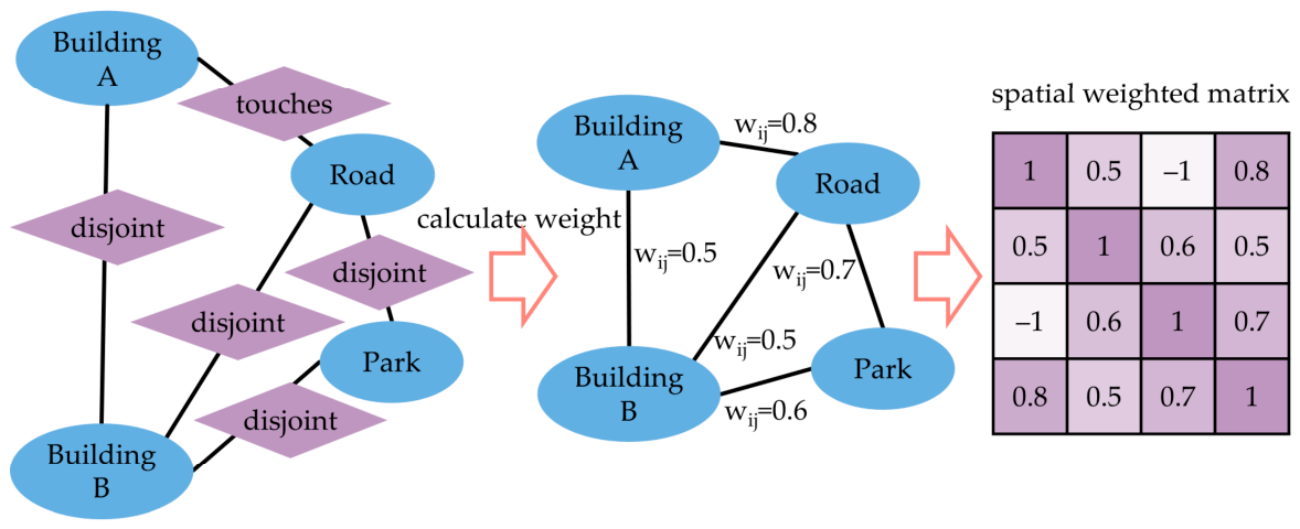
Grounded in Tobler’s First Law of Geography [48], we posit that the greater the area overlap and the shorter the distance between geographic entities, the stronger their association. Based on above principle, we quantify the association strength for each entity pair using three dimensions: area overlap, distance, and topological relation. We constructed a spatial weight matrix as a theoretical framework [49,50] to systematically describe the spatial association network among geographic entities. As shown in Figure 3, the spatial weight matrix precisely and intuitively presents the association strengths between geographic entities. The pairs of entities that are closer in distance and interact more frequently exhibit higher relationship strengths.

Definition 4.

Weight Matrix,

The weight matrix transformed spatial relationship information into continuous numerical values, using a parameterized weight function. The matrix could provide a comprehensive description of the spatial association strengths between geographic entities. The formula used for the weight matrix is shown below:

$$W=\left\{w_{ij}\right\}\in R^{n\times n},i,j\in \left\{\mathrm{1,2},\cdots ,n\right\}$$

(10)

where the matrix element $w_{ij}$ represents the spatial relationship weight between geographic entities $v_i^e$ and $v_j^e$. The n is the total number of geographic entities. The matrix W is a real-valued matrix of size n × n, denoted as $R^{n\times n}$. The weight function formula is shown below:

$$w_{ij}={\alpha }_T·\left(1+{\rho }_{ij}^{\gamma }\right)·e^{-\beta d_{ij}}$$

(11)

This function was used to comprehensively measure the spatial relationship strength across three core dimensions: topological constraints, area interaction, and distance decay. ${\alpha }_T$ represents the topological baseline weight. ${1+\rho }_{ij}^{\gamma }$ is the area interaction correction term. $e^{-\beta d_{ij}}$ is the distance decay term. The $w_{ij}$, ${\alpha }_T$, ${\rho }_{ij}$ and $d_{ij}$ are defined per unordered pair of geographic entities. For each pair ($v_i^e$, $v_j^e$), a distinct spatial relation node $v_{ij}^s$ stores its own topological relations, area interaction and distance (as shown in Formula (9) in Definition 3). Thus, an entity adjacent to multiple others spawns separate spatial relation nodes, each with independent pairwise values. The quantified weight $w_{ij}$ does not replace the original attributes (e.g., ${\rho }_{ij}$, $d_{ij}$). It synthesizes them into a single comparable value for ranking and recommendation. The original attributes remain available for other query types, preserving the full expressiveness of spatial relationships.

${\alpha }_T\in \left(0,\left.1\right]\right.$ reflects the inherent baseline association strength of different spatial topological structures. Topological relations constitute the foundational dimension for describing the spatial structure of geographic scenes. Different topological relations reflect different types of spatial associations between geographic objects. Drawing on the spatial dependency theory in geography and geometric feature analysis, we assigned baseline weights varying from 0 to 1 for various topological relations, thereby indirectly describing the strength of spatial associations. Referring to related studies on spatial correlation degree algorithms [51]. This approach adheres to the core principle that “stronger spatial dependence corresponds to higher weights.” Following this principle, we rank topological relations by the degree of shared boundary/interior: relations implying full spatial integration (e.g., “contains”, “within”) exhibit the strongest dependency, followed by partial overlap (“overlaps”, “crosses”), then boundary-level contact (“touches”), and finally complete separation (“disjoint”). Based on this ranking, we assign normalized baseline weights of 1.0, 0.9, 0.8, and 0.7 to the four topological categories, respectively. For instance, the “contains” and “within” relations represent the strongest spatial dependencies. Thus, they are assigned the maximum weight of 1 (see in

Table A1. Topological basic weight for the proposed multidimensional spatial relationship knowledge graph (MDSR-KG) model.

Predicates	Base Weight	Geometric Interpretation
equals	1.0	Two geometric objects are topologically identical
contains	1.0	Geometry B is located inside Geometry A, encompassing it
within	1.0	Geometry A is located inside Geometry B; contains coveredBy
overlaps	0.9	Two geometric objects of the same dimension partially overlap; the dimension of the intersection matches that of the objects themselves
crosses	0.9	A line crosses a surface, with the intersection being a line, or two lines intersect
touches	0.8	Two geometric objects share a boundary but do not intersect internally; they are adjacent
disjoint	0.7	Two geometric objects have no shared points; they are separate

 Appendix A for details).

In the area correction term, ${\rho }_{ij}$ represents an area interaction metric, as introduced in Section 3.3.1. ${\rho }_{ij}$ applies only to polygon-polygon pairs. For line/point geometries, or for disjoint polygon pairs, ${\rho }_{ij}=0$ and Formula (11) reduces to ${\alpha }_T·e^{-\beta d_{ij}}$. For overlapping entities, the weight receives an additional boost proportional to their intersection area. This avoids the undesirable zeroing of weights for disjoint pairs. In our Berlin dataset, only polygons are quantified; lines/points are excluded from the weight matrix but remain for other queries. Extending ${\rho }_{ij}$ to linear features is future work. The parameter $\gamma \in \left(0.1,\left.0.8\right]\right.$ denotes the area exponent coefficient. Based on the spatial interaction theory [52,53], the larger the area of contact or overlap between two geographic entities, the stronger the potential interaction. Note that the exponent coefficient regulates the nonlinearity of area influence. This parameter is tunable, and the baseline value and adjustment guidelines are introduced in Section 3.4.2.

In the distance decay term, $d_{ij}$ is the geometric distance metric introduced in Section 3.3.1. The distance decay uses minimum Euclidean distance, ignoring entity size as a simplification. We tested a normalized distance (distance divided by max circumcircle diameter), but it produced counter-intuitive rankings (e.g., a small nearby entity ranked below a large distant one). We retain Euclidean distance for geographic intuitiveness. Incorporating entity size (e.g., centroid distance) is future work. The parameter $\beta >0$ is the distance decay coefficient. The distance decay was rooted in the core idea of Tobler’s First Law of Geography, i.e., “everything is related to everything else, but near things are more related than distant things,” representing one of the most fundamental and classic theories in human geography and spatial economics [54,55]. The distance decay term quantifies the core influence of the spatial proximity of two entities on their relationship strength. The decay coefficient controls the rate at which the strength between two entities diminishes with increasing distance. This parameter’s baseline value and adjustment guidelines are introduced in Section 3.4.2.

3.4.2. Determination of Parameters

To establish scientifically grounded values for the free parameters (area exponent coefficient $\gamma$ and distance decay coefficient $\beta$) in the spatial weight matrix, we conducted a parameter calibration experiment [56,57] aimed at aligning the model’s quantitative outputs with human spatial cognition. It is important to emphasize that this calibration is conducted specifically for the Berlin dataset. The resulting values are not claimed as universally applicable. The parametric form (Equation (11)) and its tunability constitute the methodological contribution. Users can adjust these parameters according to the guidelines provided later in this section to suit different geographic contexts and analytical tasks.

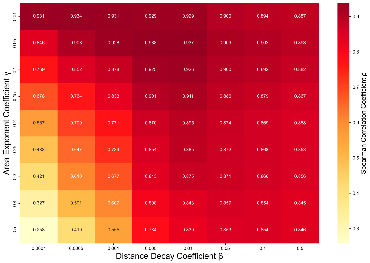
Using the Berlin OSM dataset, we constructed a calibration sample of 60 pairs of typical geographic entities, covering diverse interaction types (e.g., “building-road,” “park-water,” “school-residential area”). On the current dataset, due to the lack of independent and objective ground-truth values for ‘relationship strength’ (e.g., actual interaction frequencies such as Point of Interest(POI) visit frequency or traffic flow), we adopted expert ratings as a feasible proxy. Three geospatial analysis experts independently rated the spatial association strength for each pair on a scale from 1 (“extremely weak”) to 5 (“extremely strong”). The averaged ratings served as the ground truth for association strength [58,59]. We applied grid search [60] to optimize parameters within $\gamma \in \left[\mathrm{0.01,0.5}\right]$ and $\beta \in \left[\mathrm{0.001,0.5}\right]$, maximizing the Spearman rank correlation coefficient [61,62] between computed spatial relationship weights $w_{ij}$ and the expert ratings.

As shown in Figure 4, the maximum Spearman correlation (0.94) was achieved at $\gamma =0.05$ and $\beta =0.005$. This indicated that for this parameter combination, the quantitative ranking of spatial relationship strengths exhibited high consistency with the cognition of the human experts. The smaller $\gamma$ value suggested that area interactions exerted a relatively moderate influence on relationship strength. The smaller $\beta$ value accommodated the magnitude of distances in real-world data, ensuring that the distance decay effect operated within a reasonable spatial scale. This combination preserves model sensitivity, avoids overfitting, and exhibits strong generalization. Thus, $\gamma =0.05$ and $\beta =0.005$ were adopted as calibrated parameters (for the Berlin dataset). The topological base weight $\alpha$ was predefined according to inherent spatial dependency strengths of different topological relations (details in Table A1 in Appendix A). All subsequent analyses and experiments employed this parameter set. The above calibration serves the subsequent experiments on the Berlin dataset and is not intended to establish universally optimal parameter values.

The parameterized design of the formula endows the MDSR-KG framework with strong adaptability across diverse geographic analysis tasks. Through parameter sensitivity analysis [63,64], we derived explicit parameter adjustment guidelines for specific scenario. When addressing scenarios that required the capturing of long-range associations, such as large-scale landscape patterns, priority was given to adjusting and appropriately reducing the distance decay coefficient $\beta$. Conversely, for detailed analyses that focused on land cover boundary changes or small ecological corridors, emphasis was placed on fine-tuning the area power coefficient $\gamma$, to achieve optimal sensitivity. The framework has potential as a versatile geospatial relationship analysis tool.

To assess the robustness of the calibrated parameters (γ = 0.05, β = 0.005), we performed two complementary analyses. First, we examined the sensitivity of the Spearman correlation to parameter variations using the grid search results shown in Figure 4. Within the ranges γ ∈ [0.01,0.5] and β ∈ [0.001,0.5], the correlation remained above 0.85 for most combinations, indicating that the model’s ranking performance is not overly sensitive to the exact parameter values. Second, given the limited calibration sample (n = 60), we performed bootstrap resampling (1000 iterations) to evaluate the stability of the parameter estimates. The 95% confidence intervals are γ ∈ [0.010,0.100] and β ∈ [0.0001,0.0100], and the Spearman correlation remains above 0.88 in 95% of iterations (median ρ = 0.94). The bootstrap medians exactly match the original optimal values, confirming that the calibration is not an artifact of the specific 60-pair sample. Together, these analyses demonstrate that the parameter calibration is both stable (insensitive to sample composition) and robust (the model performs well across a range of nearby parameter values).

We acknowledge three limitations: single-city data, a small sample (60 pairs), and subjective expert ratings. The resulting values (γ = 0.05, β = 0.005) are therefore dataset-specific. The core contribution of this study remains the parametric functional form (Equation (11)) and the node-based representation paradigm, independent of specific parameter instantiations. Future work will extend the analysis to multiple geographic scales (e.g., national, global) and different application contexts (e.g., ecological assessment, urban planning), and will incorporate cross-city validation with objective interaction data (e.g., POI visit frequency, traffic flow) to further validate the framework’s adaptability.

3.4.3. Characteristics of the Quantification Model

The spatial relationship intensity quantification model proposed in this study systematically addressed the core limitations of traditional quantitative representation methods through its intrinsic mathematical design.

The quantification model achieved multidimensional integration and unified expression of spatial relationships. Rather than merely listing topological and metric dimensions in parallel, it organically integrated them within a unified mathematical framework through a parameterized weighting function. Topological relationships, overlapping areas, and distances were not isolated factors but collectively formed an interpretable and synergistic quantitative system. This inherent integration enabled the model to simultaneously respond to spatial structural, geometric, and proximity characteristics, thereby achieving a holistic representation of the complex spatial relationships across the target region.

The quantitative model exhibited mathematical interpretability and theoretical robustness. The model’s factors and computational outputs are grounded in explicit geographic significance. Users gain not only quantified relationship strengths but also valuable insights into underlying causalities, thereby supporting credible spatial decision-making.

Moreover, the model’s parametric design ensures adjustability and broad adaptability. Reference parameter values provide a robust starting point for general scenarios, while explicit theoretical guidance enables users to make precise and directional adjustments tailored to specific applications. This flexibility transforms the model from a rigid tool into a versatile analytical framework capable of adapting to diverse analytical needs and geographic scales.

4. Experiments and Results

To validate the effectiveness of the MDSR-KG framework in representing and reasoning the multidimensional spatial relationships in the region, we constructed a knowledge graph based on OSM data. Comparative experiments were conducted with representative models, such as YAGO, GeoKG, and HGeoKG, thereby providing a comprehensive evaluation with respect to the query capabilities, quantitative analysis efficiency, and computational performance.

4.1. Data Sources and Study Area

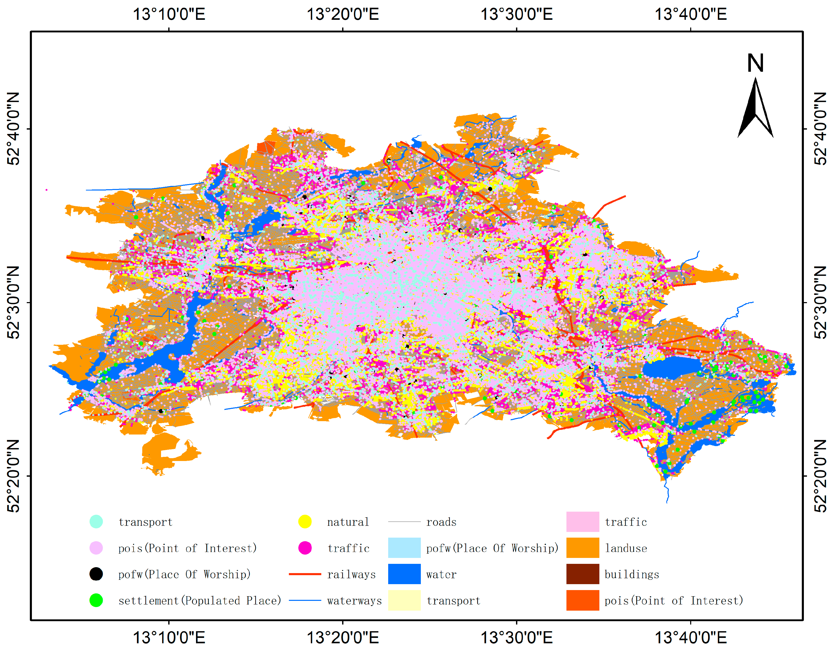
In this study, we used the OSM data for Berlin, Germany, as the experimental dataset (as shown in Figure 5). OSM is a global open-source dataset [65]. The OSM data encompassed a rich variety of vector geographic entities, along with comprehensive spatial geometric and semantic attribute information, providing an ideal data foundation for knowledge graph construction.

Table 1. Example of the OpenStreetMap (OSM) data attribute structure used in this study.

Attribute	Landuse	Water	Roads	Railways	Pois
Shape	Polygon	Polygon	Polyline	Polyline	Polygon
osm_id	4592869	4317997	4045243	4381161	4637750
code	7202	8200	5113	6102	2110
fclass	park	water	primary	light_rail	hospital
name	Ottopark	Schlachtensee	Frankfurter Allee	Berliner Stadtbahn	DRK Kliniken Berlin Mitte
ref	/	/	B1; B5	/	/
oneway	/	/	F	/	/
maxspeed	/	/	50	/	/
layer	/	/	0	1	/
bridge	/	/	F	T	/
tunnel	/	/	F	F	/

presents examples of the OSM data attribute structure. For the experiment, we extracted a large-scale dataset comprising 58,196 geographic entities and their spatial relationships, covering the core area of Berlin (Germany), to ensure the complexity and realism of the experimental scenario.

4.2. Construction of Comparative Knowledge Graphs

For the experiment, we utilized the Neo4j graph database (Community Edition 4.4) to construct and query the knowledge graphs. All code was implemented in Python 3.9 on a server with an Intel i7 CPU and 64 GB RAM [66].

Research on knowledge graph construction spans multiple technical directions, including knowledge extraction, knowledge representation, knowledge embedding, knowledge alignment and fusion, and knowledge querying and reasoning. The proposed MDSR-KG falls into the knowledge representation direction, which focuses on explicitly defining entities, relations, and their graph structures. Accordingly, we selected three representative knowledge graph models as baselines: YAGO, GeoKG, and HGeoKG. YAGO represents a general-purpose semantic knowledge graph, while GeoKG and HGeoKG are typical works in the geospatial knowledge graph domain that feature explicit spatial relation modeling. Together, they form a controlled baseline set to evaluate the core innovation of MDSR-KG: promoting spatial relations from edge structures to independent, computable nodes.

We did not include spatial database systems (e.g., PostGIS) as baselines because they target efficient geometric computation rather than relational representation, which are the focus of this study. Other technical directions, such as knowledge embedding (e.g., GeoRDF2Vec, ExpressivE) and knowledge alignment, serve different goals (e.g., link prediction, entity alignment) and are therefore not directly comparable for evaluating our representation framework.

4.2.1. Existing Models (YAGO, GeoKG, and HGeoKG)

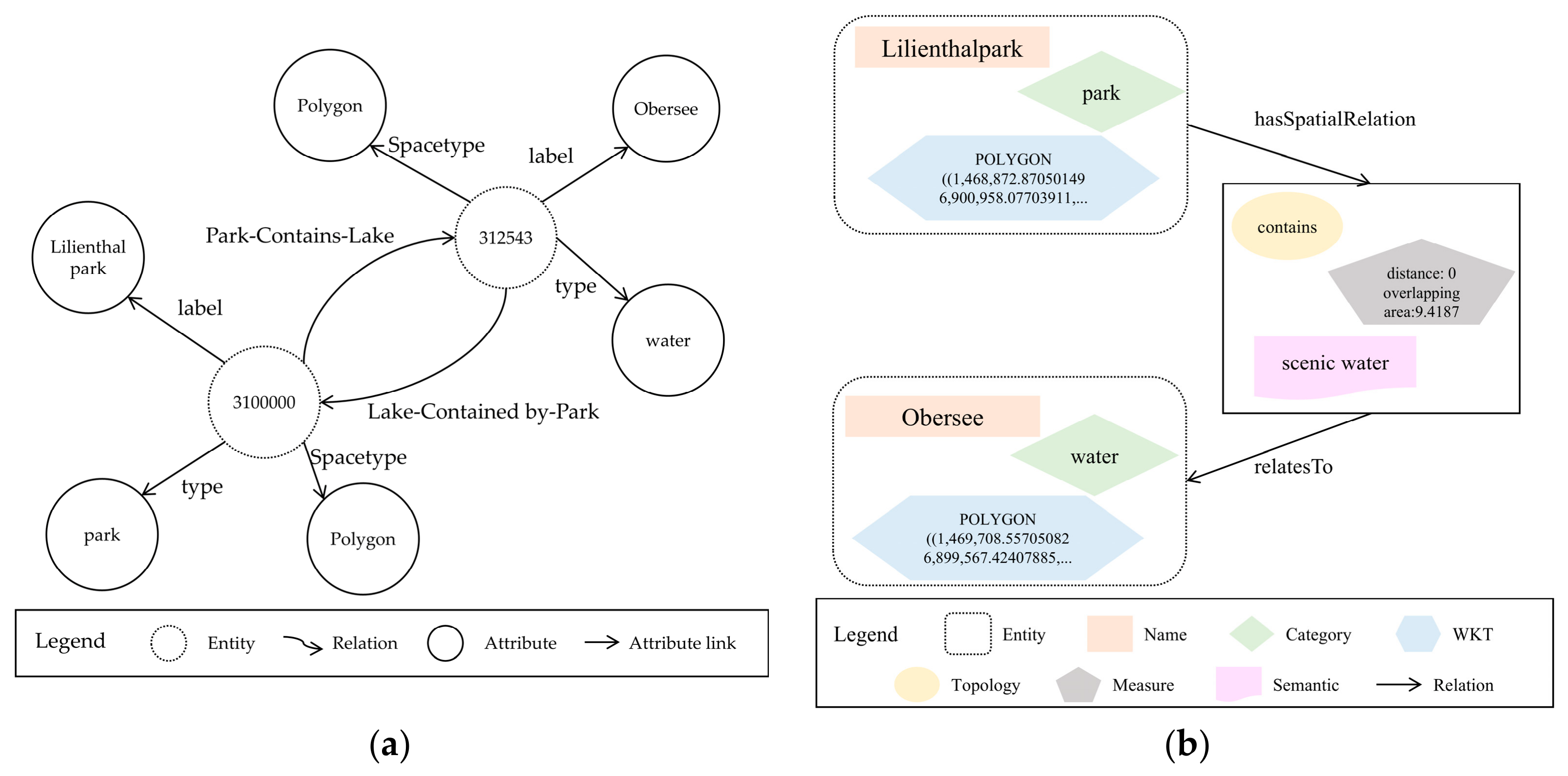
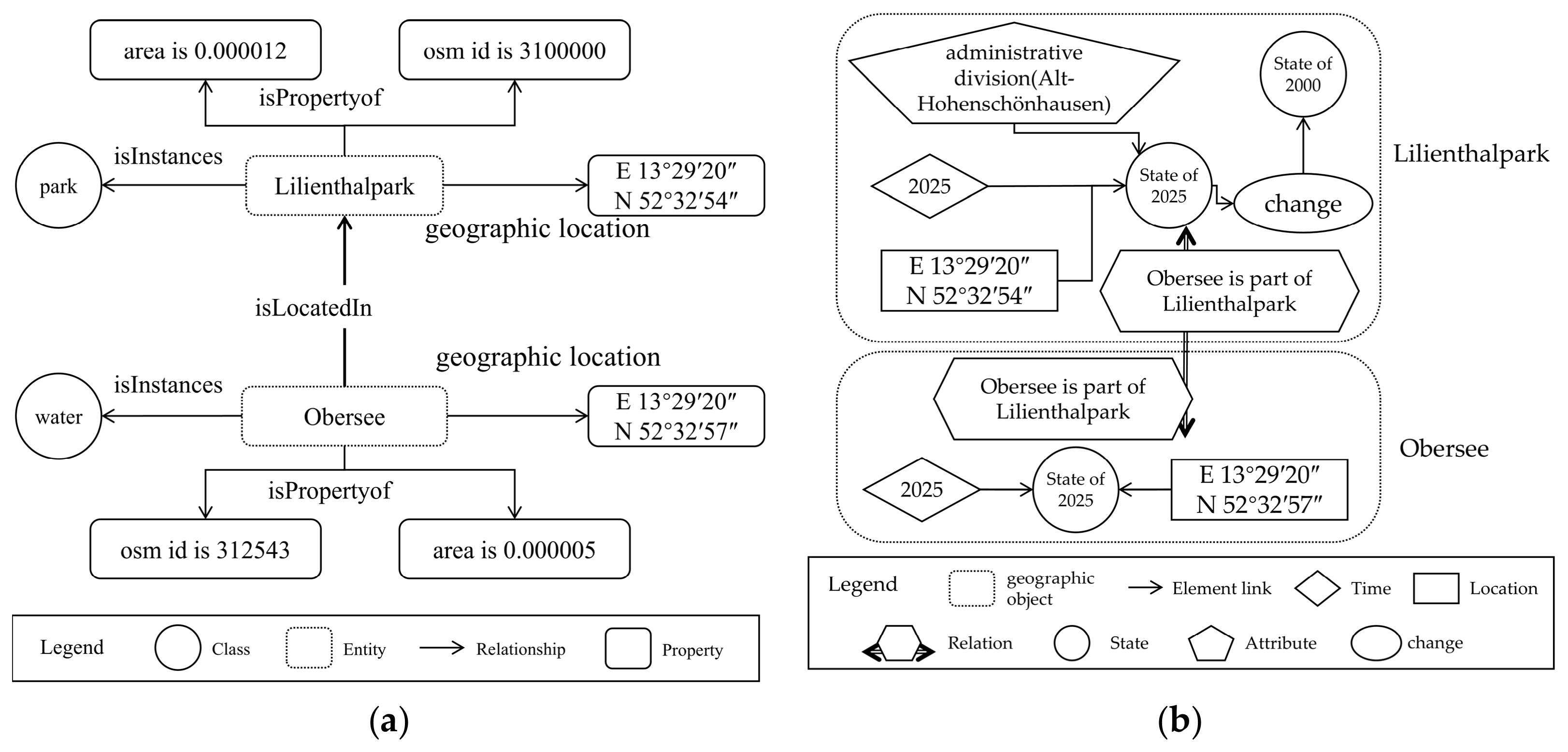
YAGO organized geographic objects using a classic triplet structure, with classes, instances, and attributes [21]. It employed semantic predicates to describe the spatial information (e.g., ‘isLocatedIn’ for administrative containment, ‘hasNeighbor’ for adjacency, and ‘hasGeoCoordinates’ for latitude/longitude). While effective for common-sense knowledge and linguistic spatial relations, YAGO lacks depth in spatial modeling, limiting support for complex spatial reasoning. Figure 6a shows an example with entities “Lilienthalpark” and “Obersee,” linked primarily via descriptive predicates like “isLocatedIn.”

GeoKG centered on the “object-state” paradigm, modeling geographic objects as state sequences [36]. Each state encompassed location, time, and attributes under specific spatiotemporal conditions. The states were connected by “change” elements, and relations described the differences between the states. However, the spatial relations (e.g., “is part of” or “is located in”) relied on predefined natural language descriptions without computable spatial models, restricting spatial querying and reasoning. Figure 6b illustrates this structure for “Lilienthalpark,” with relations categorized as spatial, temporal, or attribute-based.

HGeoKG employed a hierarchical structure, which builds regional layers based on real-world administrative divisions to organize multi-scale geographic knowledge [38]. It explicitly defined the topological relations (e.g., adjacent, contains, and intersects) by extending the DE-9IM model. It integrated common-sense entity types for multi-granularity semantics (e.g., “school-adjacent-stationery store” implying both proximity and functional association). This enables precise and semantically rich spatial representation. Figure 7a depicts an example with entities annotated by geometric and common-sense types, connected via DE-9IM-based topological relations.

4.2.2. MDSR-KG Model Proposed in This Study

In MDSR-KG, multidimensional spatial relations were computed from entity locations and geometries. Entity and spatial relation nodes were created and connected to form a structured geographic knowledge graph.

Figure 7b shows an example with entity nodes for “Lilienthalpark” and “Obersee,” including attributes (names, surface types) and geometries in WKT format—which fully captures spatial morphology beyond point coordinates. Spatial relation nodes encode topological relations (e.g., “contains”), quantitative metrics (distances, overlapping areas), and optional semantic descriptions (e.g., “landscape water body” for functional links). Entities and relations are linked via edges, forming the triple structure “geographic entity—spatial relation—geographic entity,” enabling structured representation of regional spatial relations. It should be noted that the proposed MDSR-KG explicitly models disjoint relations as independent nodes to achieve complete topological coverage. To avoid the uncontrolled growth of spatial relation nodes caused by disjoint pairs, a pruning strategy based on a distance threshold (1000 m) is applied during graph construction. In the Berlin dataset, the spatial weight between entity pairs separated by more than 1000 m approaches zero. These pairs are considered to have negligible spatial interaction, and thus no relation node is created for them. This threshold is dataset-specific and may be adjusted for other geographic contexts (e.g., sparser rural areas).

4.3. Results and Analysis

To systematically evaluate the MDSR-KG model’s capabilities in geospatial knowledge representation and reasoning, we conducted experiments in three dimensions: spatial query capability, relationship strength inference, and scalability. These addressed key questions: (1) expressive completeness and accuracy in multidimensional complex spatial queries; (2) application of relationship strength quantification in ranking and recommendation tasks; and (3) usability in real-world scenarios.

4.3.1. Comparison of Expressive Power

This section evaluates the expressive power of each model—i.e., what types of spatial queries can be formulated and correctly answered. We used 20 representative spatial query tasks, divided into simple (single spatial relationship constraint) and composite queries (multiple conditions). Tasks covered topology, metric, and semantic dimensions to evaluate query expressiveness [67,68]. Queries were executed using Cypher (Neo4j’s query language) on the property graph..

Table 2. Query types supported by each model *.

Models	Semantic Query	Topology Query	Metric Query	Composites Query	Supported Count
YAGO	✓ (limited predicates)	✗	✗	✗	1
GeoKG	✓	✓ (limited predicates)	✗	✗	2
HGeoKG	✓ (entity attributes)	✓	✗	✗	2
MDSR-KG	✓	✓	✓	✓	4

* Note: ✓ indicates that the model supports queries in this dimension. ✗ indicates that it does not.

summarizes the query types supported by each model. In YAGO, spatial relations are described using predicates such as isLocatedIn, containedIn, contains, isConnectedTo, and isAdjacentTo; thus it only supports semantic queries. GeoKG uses predicates for semantics (isStateof, isLocationof) and topology (located in, south of, passes through), but lacks metric descriptions. HGeoKG includes entity attributes and categories for semantics, while its spatial relations are based solely on DE-9IM topology. MDSR-KG is the only framework that supports all four types—topology, semantics, metrics, and composites—enabling it to handle complex spatial queries that baseline models cannot express.

Table 3. Comparison of accuracy on supported queries *.

Models	F1 Score	Explanation
YAGO	0.83	Semantic predicates approximate topology (e.g., ‘hasNeighbor’ for ‘disjoint’); coarse categories cause over-inclusion
GeoKG	0.89	Missing ‘disjoint’ relations; sparse relation instances reduce recall
HGeoKG	0.89	Missing ‘disjoint’ relations; sparse relation instances
MDSR-KG	0.99	Multidimensional attributes ensure precise matching

* Note: This comparison is based on the subset of queries that all models can support (i.e., pure topological and semantic queries).

evaluates performance on the subset of queries that all models can support. To provide a fair comparison of accuracy, this comparison is based on the 13 queries that all four models can execute. Metric and composite queries involving distance or direction are excluded because baseline models cannot represent them. This avoids conflating expressive power with query correctness. The small performance gap on common queries confirms that MDSR-KG’s superior expressive power does not come at the cost of accuracy on basic tasks.

The sub-perfect F1 scores for models stem from their intrinsic representational limits. YAGO uses semantic predicates to approximate topology (e.g., ‘hasNeighbor’ for disjoint) and coarse categories that over-include results. GeoKG and HGeoKG omit certain topological relations (e.g., disjoint) and have sparse relation instances. MDSR-KG avoids these issues by direct attribute encoding, achieving 0.99.

Table 4. Query examples.

Type	Query Task	YAGO	GeoKG	HGeoKG	MDSR-KG	Correct Answer
Simple query	Q_A: Which residential entities are within 100 m of the school called Manfred-Von-Ardenne Gymnasium?	Cannot execute. No distance metric support.	Cannot execute. No distance metric support.	Cannot execute. No distance metric support.	Returns all 8 entities via distance attribute (dij ≤ 100 m).	8 entities (OSM IDs: 1231750611, 1231750614, 1231750615, 1231750617, 1231754163, 1231754164, 46931506, 46931556)
Simple query	Q_B: What is the spatial relationship between park “Oberseepark” and kindergarten “Kitaverbund Regenbogen”?	Returns “hasNeighbor”.	Returns “near by”.	No result. HGeoKG does not record disjoint relations.	Returns “disjoint” via topological attribute.	disjoint
Complex query	Q_C: Which commercial entities are within 100 m of a river and are adjacent to a park?	Cannot execute. Cannot represent metric constraint.	Cannot execute. Cannot represent metric constraint.	Cannot execute. Cannot represent metric constraint.	Returns the correct entity via combined filtering on distance (d_ij ≤ 100 m) and topology (touches).	1 entity (OSM ID: 419912417)

presents three representative queries that highlight the key differences in expressive power among the models. The full list of 20 query tasks is provided in in

Table A2. All Query task.

Type	Query Task	Model Expressiveness
Simple query	Q1: Which park has name “Park an der Spree”?	All models return correct result.
	Q2: Find all buildings of type “hospital”.	All models return correct results.
Simple query	Q3: Which water is located in park “Oberseepark”?	All models return correct result (YAGO via predicate isLocatedIn; GeoKG via predicate isPartOf; HGeoKG via topological contains; MDSR-KG via topological contains).
Simple query	Q4: Which roads are adjacent to a given residential building?	All models return correct results (YAGO/GeoKG via isAdjacentTo; HGeoKG via Adjacent; MDSR-KG via topological touches).
Simple query	Q5: Retrieve the road network of “Ebertstraße”.	All models return correct results (31 road segments).
Simple query	Q6: Which administrative district a given building belongs to?	Only HGeoKG includes administrative hierarchy data; YAGO/GeoKG/MDSR-KG lack this data in the current experiment.
Simple query	Q7: What is the spatial relationship between park “Oberseepark” and kindergarten “Kitaverbund Regenbogen”?	YAGO returns “hasNeighbor”; GeoKG returns “near by” and HGeoKG return no result (disjoint not recorded); MDSR-KG returns “disjoint”.
Simple query	Q8: Which residential entities are within 100 m of the school called Manfred-Von-Ardenne Gymnasium?	Only MDSR-KG can execute (via distance attribute). YAGO/GeoKG/HGeoKG cannot represent metric constraints.
Simple query	Q9: Which roads are located south of water body “Papenpfuhlbecken”?	YAGO and HGeoKG cannot execute (no direction support); GeoKG returns correct results via “is south of”; MDSR-KG returns correct results via semantic south.
Simple query	Q10: What green areas inside park “Oberseepark”?	YAGO/GeoKG/HGeoKG cannot execute (no semantic tag for green area); MDSR-KG returns correct results via semantic attribute.
Complex query	Q11: Which hospital adjacent to commercial buildings?	All models return correct result (via adjacency predicates or touches topological attribute).
Complex query	Q12: Which commercial entities contain supermarket?	All models return correct results (via containment predicates or contain topological attribute).
Complex query	Q13: Which park contain both a lack and a forest?	All models return correct results (via containment predicates or contain topological attribute).
Complex query	Q14: Find parks located along a river and also having a fountain.	YAGO returns over-inclusive results (due to coarse category ‘BodyOfWater’); GeoKG and HGeoKG return correct result; MDSR-KG returns correct result.
Complex query	Q15: What lack is inside Tiergarten park within the Mitte district of Berlin?	Only HGeoKG includes administrative hierarchy data; YAGO/GeoKG/MDSR-KG lack this data in the current experiment.
Complex query	Q16: Find residential areas that are close to a main road and adjacent to a park.	YAGO returns partial results (using hasNeighbor as proxy); GeoKG and HGeoKG return fewer results (sparse relation instances); MDSR-KG returns all correct results (via combined topological and metric attributes).
Complex query	Q17: Which residential entities is within 50 m of school “John-Lennon-Gymnasium” and also near a park?	Only MDSR-KG can execute (metric constraint). YAGO/GeoKG/HGeoKG cannot represent distance.
Complex query	Q18: Which commercial entities are within 100 m of a river and is adjacent to a park?	Only MDSR-KG can execute (combined metric and topological constraint). YAGO/GeoKG/HGeoKG cannot represent metric constraints.
Complex query	Q19: Find the location of water towers located inside parks.	All models return correct result.
Complex query	Q20: Find names of all schools that have a kindergarten nearby.	YAGO returns over-inclusive results (due to coarse category ‘EducationalInstitution’); GeoKG and HGeoKG return correct results; MDSR-KG returns correct results.

 Appendix B. For metric and topological queries (Q_A and Q_B), baseline models either return no results or produce inaccurate outputs, while MDSR-KG delivers precise answers. For composite queries (Q_C) requiring both metric and topological constraints, only MDSR-KG can integrate both dimensions.

4.3.2. Verifying the Reasoning Capability of the Relationship Strength Quantification

To validate the practical value of the quantitative calculation module in the MDSR-KG model, we designed ranking and recommendation tasks. This is not a comparative experiment but rather a demonstration and application of the relationship strength quantification capability within the MDSR-KG model. These tasks required the models to quantitatively assess the strength of the relationship and to rank and prioritize the associated entities accordingly. This capability is crucial for applications that require precise quantitative basis (e.g., land cover hotspot identification and urban facility siting) [69,70,71,72].

We constructed six tasks covering “influence ranking” (identifying strongest interactions for environmental impact) and “suitability recommendation” (balancing multiple relationships in site selection; details in

Table 5. Examples of the ranking and suitability recommendation tasks.

Task Type	Task
influence ranking	A1 (Ecological Influence): Identify the three water bodies with the greatest environmental influence on the park “Volkspark Friedrichshain”.
	A2 (Traffic Influence): Identify the three roads most critical to the traffic accessibility of the major commercial facility (OSM ID: 138554287).
	A3 (Service Influence): Identify the three commercial facilities that provide the most essential services to the residential area (OSM ID: 47722627).
suitability recommendation	B1 (Emergency Facility Siting): Recommend three optimal locations for a new fire station to enable the fastest response to multiple high-density residential areas.
	B2 (Commercial Facility Siting): Recommend three optimal locations for a new large supermarket, ensuring proximity to residential areas and convenient truck access (close to major roads).
	B3 (Public Space Siting): Recommend three optimal locations for a new community park, ensuring service to multiple residential areas while maintaining a quiet environment (away from major roads).

).

For analogous scenario tasks, spatial data processing tools (e.g., GIS) are capable of performing calculations such as distance measurement and buffer generation. However, they are unable to integrate multidimensional factors—including topological relations, spatial distance, and functional semantics—to conduct a comprehensive ranking analysis, and they lack the automated reasoning capabilities inherent to knowledge graphs. The baseline models (YAGO, GeoKG, and HGeoKG) lacked a continuous relations strength metric. Employing a simple heuristic ranking based on topological types (e.g., contains > touches > disjoint) results in a large number of features being assigned the same rank, thereby failing to produce a meaningful ordering. Conversely, performing real-time computations based on spatial geometry would require manually designing complex workflows for each individual task, rendering direct comparison both inequitable and meaningless. This underscores limitations of traditional paradigms in advanced spatial reasoning. We acknowledge that objective ground truth for ranking and recommendation tasks (e.g., real-world fire station response times or ecological impact data) is often unavailable or difficult to obtain. We thus used qualitative case studies and expert evaluation for MDSR-KG. Significance testing and objective external metrics are not included and are left for future work.

MDSR-KG generated recommendations based on spatial weight. Three experts from the field of Geographic Information Science, each with over five years of research experience, were selected. Each expert first independently performed the ranking/recommendation tasks based on their own analysis of the OSM data, and the results with majority agreement were taken as a reference (as shown in the ‘Results of expert’ column in

Table 6. Case results and expert evaluation for the spatial relationship strength ranking task.

Task	Results of MDSR-KG (OSM ID, Type, Name)	Results of Expert (Reference) (OSM ID, Type, Name)	Expert Ratings (E1,E2,E3) *	Mean Score
A1	1. (53477, water, null) 2. (1628978, water, null) 3. (53487, water, null)	1. (26993, water, Neuer See) 2. (53477, water, null) 3. (1628978, water, null)	(4,4,3)	3.67
A2	1. (1132163645, tertiary, Friedrichstrae) 2. (387125525, subway, U6) 3. (753316505, tertiary, Glinkastrae)	1. (387125525, subway, U6) 2. (1132163645, tertiary, Friedrichstrae) 3. (753316505, tertiary, Glinkastrae)	(5,5,5)	5.0
A3	1. (478632893, commercial, null) 2. (478633215, commercial, null) 3. (18630167, commercial, null)	1. (478632893, commercial, null) 2. (18630167, commercial, null) 3. (478632299, commercial, null)	(4,4,4)	4.0
B1	1. (1305456605, residential, null) 2. (1305456602, residential, null) 3. (1305456606, residential, null)	1. (1305456605, residential, null) 2. (1305456606, residential, null) 3. (1305506226, residential, null)	(4,4,3)	3.67
B2	1. (25807904, commercial, MEON-Gewerbepark) 2. (1064294301, commercial, null) 3. (1077364415, commercial, null)	1. (25807904, commercial, MEON-Gewerbepark) 2. (1064294301, commercial, null) 3. (1077364415, commercial, null)	(5,5,5)	5.0
B3	1. (1295122233, residential, null) 2. (1295300270, residential, null) 3. (1295257439, residential, null)	1. (1295300270, residential, null) 2. (1295122239, residential, null) 3. (1295122240, residential, null)	(3,3,3)	3.0
Overall mean				4.06

* Note: The three experts were from the field of Geographic Information Science, with over five years of experience in geographic information data research. Fleiss’ Kappa = 0.664, indicating substantial inter-rater agreement.

). The reference results are provided for comparison, not as ground truth. Then, they rated the reasonableness of each MDSR-KG output on a 5-point scale (5: highly reasonable and decision-applicable; 4: plausible; 3: partially reasonable with bias; ≤2: largely unreasonable) [73]. Finally, the mean expert rating and Kappa coefficient were calculated for each task to evaluate the effectiveness of the model’s quantitative module.

MDSR-KG averaged 4.06 across tasks (Table 5), confirming recommendation validity and practicality. The Kappa value is 0.664, indicating substantial inter-rater agreement. In influence ranking, it identified strong entities and quantified differential contributions. Here, “influence” refers to the quantified ecological impact of spatial entities (e.g., water bodies or parks) within the knowledge graph, derived from multidimensional factors including topological connectivity (base weights distinguishing internal vs. external features) and attribute metrics (e.g., area size). For instance, in A1, it captured that internal water bodies exert greater ecological influence than adjacent external ones (via topological base weight) and refined rankings within parks using area metrics. This reflects synergistic inference from multidimensional relationships and attributes, ensuring rigor and interpretability. In suitability recommendation, it balanced complex constraints effectively, recommending nodes with optimal connectivity rather than mere geometric centers. In B2, it optimized proximity to residential areas and roads, aligning perfectly with experts. In B3, lower scores reflected real-world trade-offs (service coverage vs. quietness), mitigated by metrics like distance decay and area correction. These results show MDSR-KG’s quantification enables evolution from query tools to interpretable spatial intelligence platforms supporting quantifiable decision-making and novel reasoning.

4.3.3. Scalability Analysis of the Proposed Model

We systematically evaluated the model’s scalability and performance overhead to evaluate its feasibility in practical large-scale applications [74]. The MDSR-KG model is verified that the performance cost was fixed and controllable, rather than being a catastrophic overhead that escalated with scale.

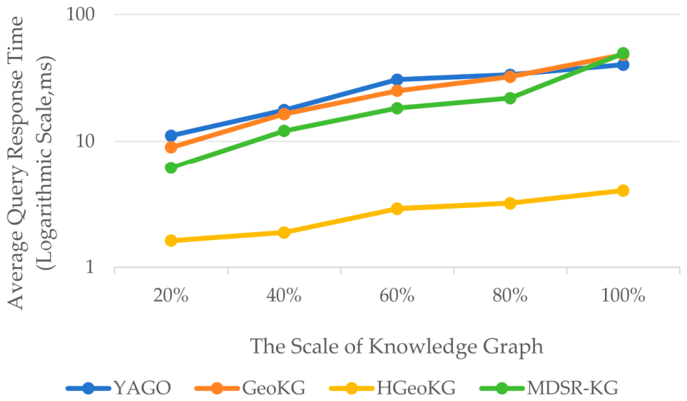
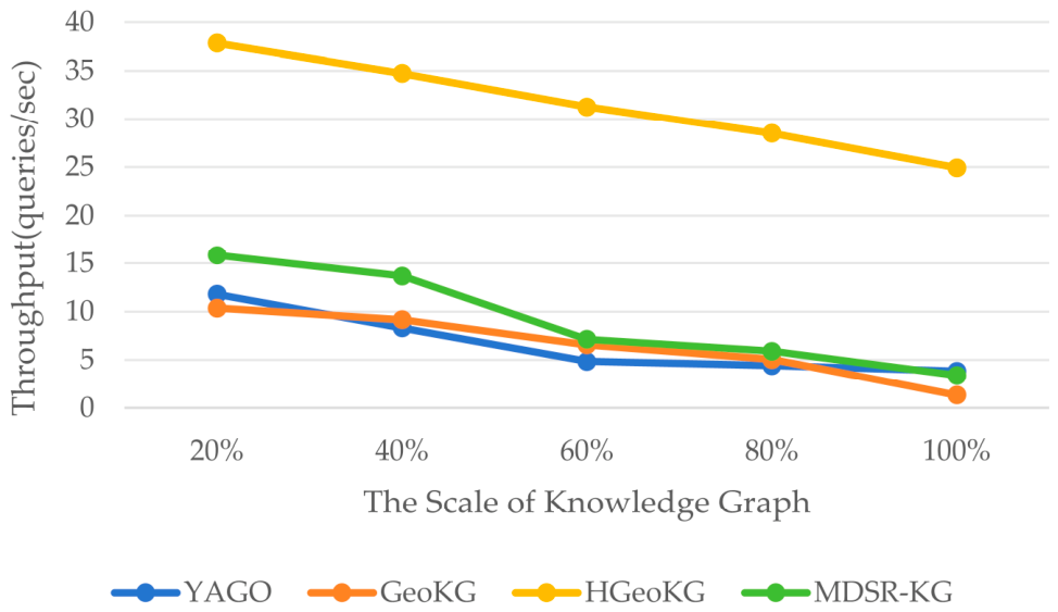
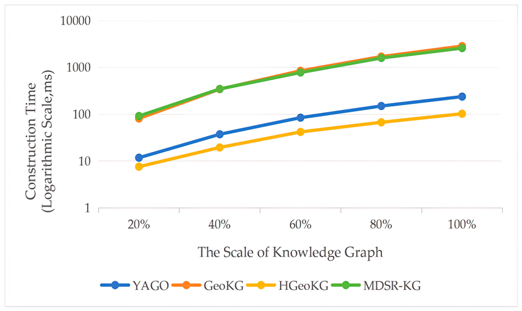
We generated five subsets (S1–S5) from Berlin OSM data (20–100% scale; 11,000–58,000 entities) via random entity sequences. All models were constructed using the same geographic entities from these subsets, resulting in varying numbers of nodes and edges. However, due to their different representational designs (e.g., whether spatial relations are reified as independent nodes), the resulting knowledge graphs exhibit varying numbers of nodes and edges, as summarized in Table 6 for the 100% scale. These differences reflect inherent structural choices rather than variations in data coverage or processing success. A fixed set of representative queries measured average response time, total execution time, and throughput. All models were successfully constructed and executed all queries on every subset. This emphasized traversal efficiency over expressive boundaries. To ensure fairness and scientific rigor in model comparison, the query tasks were restricted to those supported by all models, relying primarily on the basic topological and predicate semantic relationships of the region. To evaluate the scalability rather than revalidate expressive power of each model, we selected a set of representative sample queries (e.g., Q1, Q4, and Q5; explained in Section 4.3.1) that all models could execute efficiently. In unified environments, tasks were executed 10 times per batch; results are in Table 6 and Figure 8 and Figure 9.

Table 6 shows MDSR-KG’s higher node/edge counts due to relation instantiation, reflecting overhead for multidimensional representation. Owing to the distance threshold constraint, the number of spatial relation nodes per geographic entity has a theoretical upper bound; consequently, the total number of nodes grows approximately linearly with the number of entities, rendering the increase in scale manageable. Figure 8 indicates sublinear response time growth for all models; MDSR-KG’s higher absolute times paralleled baselines, with overhead as a fixed factor from traversal complexity. Figure 9 shows steady throughput decline, confirming excellent scalability for all, including MDSR-KG. Figure 10 shows the construction time for each model on the five subsets (S1–S5). The approximately linear growth of construction time is acceptable.

Based on the results, HGeoKG achieved best (millisecond) performance; YAGO averaged 40.21 ms due to simple structure; GeoKG matched MDSR-KG via comparable complexity. MDSR-KG’s relation-node design increases traversal but enables complex queries and quantitative reasoning—a valuable trade-off exchanging controlled cost for expressive gains, common in complex systems [75,76,77]. Crucially, the performance cost incurred by the MDSR-KG model was fixed and controllable, remaining manageable even with the expansion of the graph scale. Its robust scalability fully demonstrated the framework’s feasibility for practical geospatial analysis applications.

Notably, the performance comparison between the models showed significant differences in their inherent “completeness of relationship representation.” As shown in the graph scale data (

Table 7. Data scale and performance benchmarks for models at 100% scale gradient *.

Model	Nodes Count	Edges Count	Construction Time (s)	Average Query Response Time (ms)	Total Execution Time (s)	Throughput (Queries/s)
MDSR-KG	18,166,522	36,216,652	2592.02	49.41	8.85	3.38
HGeoKG	58,205	258,837	102.61	4.05	1.20	24.91
GeoKG	174,588	18,224,718	2859.45	48.19	22.08	1.35
YAGO	58,196	2,068,143	238.49	40.21	7.82	3.83

* Note: Node/edge counts reflect model design, not processing success. All models used the same entities per scale.

), the MDSR-KG model possessed the most complex graph structure. This complexity stemmed from its design objective: to capture and represent the diverse spatial interactions between geographic entities as comprehensively as possible (e.g., “disjoint” that were overlooked by baseline models). Consequently, the graph processed by the MDSR-KG model exhibited higher information density and complexity. It justified simple-query penalties for unattainable advanced tasks (Section 4.3.1 and Section 4.3.2). Although MDSR-KG incurs a fixed performance cost on simple queries, this is exchanged for a qualitative leap in the expressiveness and reasoning capabilities of spatial relations. At the same time, we acknowledge that the current experiments are based solely on the Berlin city dataset. Further validation on larger-scale (e.g., national or global) datasets remains necessary. Nevertheless, with the distance-based pruning strategy, the number of spatial relation nodes grows approximately linearly with the number of entities, which is a manageable scaling behavior. Moreover, our experiments on datasets of increasing size (up to 58,000 entities) have demonstrated that the performance overhead remains controllable. Therefore, the current results already support the framework’s feasibility for city- and regional-scale applications. We also acknowledge that storage optimization (e.g., compact encoding of spatial relation nodes) is not addressed in the current study. This is important direction for future work to further improve scalability.

4.4. Discussion

The experimental evaluation systematically validated the effectiveness and advancement of the MDSR-KG framework in expressive capability, reasoning capability, and scalability. Results quantified its superiority over baseline models, showing that the MDSR-KG drive a shift in geographic knowledge graphs—from static relation storage to dynamic relation understanding and computation.

First, MDSR-KG’s core advantage lies in elevating spatial relations to independent nodes. When using complex spatial queries in Section 4.3.1, the MDSR-KG model’s spatial relational nodes (as structured and addressable entities) enable direct querying and filtering of relationships themselves (e.g., “find all spatial relationships with interaction strength > X”). This shifts knowledge graphs from simple connections to platforms supporting deep spatial interaction interpretation, validating the theoretical framework in Section 3.

Second, relationship strength quantification of MDSR-KG highlighted strong potential for spatial decision-making support. As demonstrated in Section 4.3.2, the spatial relationship descriptions of the baseline models can no longer meet the demands for refinement and interpretability in modern spatial analysis. The “quantitative calculation module” of the MDSR-KG advanced from “existence identification” to “strength understanding and causes.” It provides quantitative tools for applications like urban planning, environmental assessment, and land cover classification, while establishing an interpretable framework for advanced spatial modeling.

Scalability analysis confirms MDSR-KG’s engineering feasibility, achieving a favorable balance in the expressiveness-efficiency trade-off. As demonstrated in Section 4.3.3, MDSR-KG trades a controllable additional computational overhead for the ability to address complex problems beyond the capabilities of baseline models, while clearly delineating the applicability boundaries of different models. MDSR-KG demonstrates strong scalability as a practical framework for city- and regional-scale spatial analysis.

5. Conclusions

This study addresses the core limitations of existing geographic knowledge graphs—monodimensional spatial relationship representation, insufficient quantification methods, and weak complex reasoning capabilities—by proposing the MDSR-KG framework. Through the innovative “spatial relation node” and a parameterized relationship strength quantification model, MDSR-KG achieves an advancement from merely detecting “whether a relationship exists” to assessing “how strong the relationship is and why.” Systematic comparative experiments confirm MDSR-KG’s superior performance in expressive power for complex spatial queries and reasoning capability for relationship strength ranking, while demonstrating excellent scalability on real-world city- and regional-scale datasets. This bridges the gap between theoretical innovation and practical engineering application. The study provides a viable pathway for computationally representing human geospatial cognition.

Despite promising results, several limitations remain. Primarily, in the computational process of quantifying spatial relationship strength, the setting of parameters entails a certain degree of subjectivity. More objective calibration methods (e.g., learning from data) remain future work. Second, the enhanced expressive power of MDSR-KG comes with increased computational complexity, necessitating future exploration of targeted graph indexing and query optimization techniques to improve usability. Third, the current framework still offers an incomplete description of spatial relationships. The temporality and directional relations are critical dimensions in geographic analysis. A promising direction is to explicitly incorporate the temporal and directional dimension by developing spatiotemporal relation nodes that encode both relationship strength and evolutionary patterns, enabling unified modeling of dynamic geographic interactions. Additionally, the experiments relied on OSM vector data; future work could integrate multimodal remote sensing imagery, addressing vector-raster alignment and joint computation to construct multimodal geospatial knowledge graphs and evaluate their performance in complex real-world scenarios. Finally, integrating MDSR-KG with cutting-edge AI technologies, particularly leveraging its structured spatial knowledge to enhance large language models’ geospatial reasoning and mitigate spatial cognitive biases, offers significant research potential. This could advance the development of next-generation geospatial agents capable of understanding and solving complex spatial problems.

References

1. Hou, Z.-W.; Liu, X.; Zhou, S.; Jing, W.; Yang, J. Bibliometric Analysis on the Research of Geoscience Knowledge Graph (GeoKG) from 2012 to 2023. ISPRS Int. J. Geo-Inf. 2024, 13, 255. [Google Scholar] [CrossRef]
2. Ghazouani, F.; Farah, I.R.; Solaiman, B. A Multi-Level Semantic Scene Interpretation Strategy for Change Interpretation in Remote Sensing Imagery. IEEE Trans. Geosci. Remote Sens. 2019, 57, 8775–8795. [Google Scholar] [CrossRef]
3. Phengsuwan, J.; Shah, T.; James, P.; Thakker, D.; Barr, S.; Ranjan, R. Ontology-Based Discovery of Time-Series Data Sources for Landslide Early Warning System. Computing 2020, 102, 745–763. [Google Scholar] [CrossRef]
4. Potnis, A.V.; Durbha, S.S.; Shinde, R.C.; Talreja, P.V. Towards Visual Exploration of Semantically Enriched Remote Sensing Scene Knowledge Graphs (RSS-KGs). In Proceedings of the 2021 IEEE International Geoscience and Remote Sensing Symposium IGARSS, Brussels, Belgium; IEEE: New York, NY, USA, 2021; pp. 5783–5786. [Google Scholar]
5. Zhang, J.; Gu, H.; Yang, Y.; Zhang, H.; Li, H. Research Progress and Trend of High-Resolution Remote Sensing Imagery Intelligent Interpretation. Natl. Remote Sens. Bull. 2021, 25, 2198–2210. [Google Scholar] [CrossRef]
6. Hao, L.; Mei, X. Exploring the Use of Virtual Geographic Environments for Geo-Spatial Cognition Research. Natl. Remote Sens. Bull. 2021, 25, 2027–2039. [Google Scholar] [CrossRef]
7. Montello, D.R. Cognition of Geographic Information. In A Research Agenda for Geographic Information Science; CRC Press: Boca Raton, FL, USA, 2004; pp. 61–91. [Google Scholar]
8. Shoorcheh, M. On the Spatiality of Geographic Knowledge. Asian Geogr. 2019, 36, 63–80. [Google Scholar] [CrossRef]
9. Nations, U. Transforming Our World: The 2030 Agenda for Sustainable Development. Available online: https://sdgs.un.org/2030agenda (accessed on 2 April 2026).
10. Wang, S.; Han, W.; Zhang, X.; Li, J.; Wang, L. Geospatial Remote Sensing Interpretation: From Perception to Cognition. Innov. Geosci. 2024, 2, 100056. [Google Scholar] [CrossRef]
11. Zheng, K.; Xie, M.H.; Zhang, J.B.; Xie, J.; Xia, S.H. A Knowledge Representation Model Based on the Geographic Spatiotemporal Process. Int. J. Geogr. Inf. Sci. 2022, 36, 674–691. [Google Scholar] [CrossRef]
12. Ma, X.; Ma, C.; Wang, C. A New Structure for Representing and Tracking Version Information in a Deep Time Knowledge Graph. Comput. Geosci. 2020, 145, 104620. [Google Scholar] [CrossRef]
13. Ma, X. Knowledge Graph Construction and Application in Geosciences: A Review. Comput. Geosci. 2022, 161, 105082. [Google Scholar] [CrossRef]
14. Janowicz, K.; Hitzler, P.; Li, W.; Rehberger, D.; Schildhauer, M.; Zhu, R.; Shimizu, C.; Fisher, C.; Cai, L.; Mai, G. Know, Know Where, KnowWhereGraph: A Densely Connected, Cross-Domain Knowledge Graph and Geo-Enrichment Service Stack for Applications in Environmental Intelligence. AI Mag. 2022, 43, 30–39. [Google Scholar] [CrossRef]
15. Géraldine, D.M.; Peng, P.; Jérôme, G.; Christophe, C.; Feng, L. Leveraging Spatio-Temporal Graphs and Knowledge Graphs: Perspectives in the Field of Maritime Transportation. ISPRS Int. J. Geo-Inf. 2021, 8, 541. [Google Scholar] [CrossRef]
16. Shbita, B.; Knoblock, C.A.; Duan, W.; Chiang, Y.Y.; Uhl, J.H.; Leyk, S. Building Spatio-Temporal Knowledge Graphs from Vectorized Topographic Historical Maps. Semant. Web 2023, 14, 527–549. [Google Scholar] [CrossRef]
17. Qiu, P.; Jialiang, G.; Li, Y.; Feng, L. Knowledge Embedding with Geospatial Distance Restriction for Geographic Knowledge Graph Completion. ISPRS Int. J. Geo-Inf. 2019, 6, 254. [Google Scholar] [CrossRef]
18. Cui, W.; Yao, M.; Hao, Y.; Wang, Z.; He, X.; Wu, W.; Li, J.; Zhao, H.; Xia, C.; Wang, J. Knowledge and Geo-Object Based Graph Convolutional Network for Remote Sensing Semantic Segmentation. Sensors 2021, 21, 3848. [Google Scholar] [CrossRef] [PubMed]
19. Liu, D. Study construction of the geo-entities database—Major in rivers. Master’s Thesis, Shandong University of Science and Technology, Qingdao, China, 2010. [Google Scholar]
20. Yue, Z.; Zhong, S.; Mei, X. Research on Complex Spatiotemporal Semantic Modeling Integrating Spatial Data Engines and Graph Databases. J. Geo-Inf. Sci. 2025, 27, 1289–1304. [Google Scholar]
21. Suchanek, F.M.; Alam, M.; Bonald, T.; Chen, L.; Paris, P.-H.; Soria, J. Yago 4.5: A Large and Clean Knowledge Base with a Rich Taxonomy. In Proceedings of the 47th International ACM SIGIR Conference on Research and Development in Information Retrieval, Washington, DC, USA; Association for Computing Machinery: New York, NY, USA, 2024; pp. 131–140. [Google Scholar]
22. Lehmann, J.; Isele, R.; Jakob, M.; Jentzsch, A.; Kontokostas, D.; Mendes, P.N.; Hellmann, S.; Morsey, M.; Van Kleef, P.; Auer, S. Dbpedia–a Large-scale, Multilingual Knowledge Base Extracted from Wikipedia. Semant. Web 2015, 6, 167–195. [Google Scholar] [CrossRef]
23. Ning, Y.; Liu, H. UrbanKGent: A Unified Large Language Model Agent Framework for Urban Knowledge Graph Construction. In Proceedings of the NeurIPS 2024, Annual Conference on Neural Information Processing Systems 37, Vancouver, Canada; Curran Associates, Inc.: New York, NY, USA, 2024. [Google Scholar]
24. Hu, L.; Li, W.; Xu, J.; Zhu, Y. GeoEntity-Type Constrained Knowledge Graph Embedding for Predicting Natural-Language Spatial Relations. Int. J. Geogr. Inf. Sci. 2025, 39, 376–399. [Google Scholar] [CrossRef]
25. Guo, C.; Xu, T.; Liu, L. Construction of Knowledge Graph Based on Geographic Ontology. In Proceedings of the IOP Conference Series: Earth and Environmental Science; IOP Publishing: Philadelphia, PA, USA, 2019; p. 052161. [Google Scholar]
26. Du, J.; Wang, S.; Ye, X.; Sinton, D.S.; Kemp, K. GIS-KG: Building a Large-Scale Hierarchical Knowledge Graph for Geographic Information Science. Int. J. Geogr. Inf. Sci. 2022, 36, 873–897. [Google Scholar] [CrossRef]
27. Zhang, B.; Yin, C.; Liu, K.; Zhai, X.; Sun, Y.; Du, M. Research on the Construction of Geographic Knowledge Graph Integrating Natural Disaster Information. ISPRS Ann. Photogramm. Remote Sens. Spat. Inf. Sci. 2022, 10, 79–85. [Google Scholar] [CrossRef]
28. Lovera, F.; Cardinale, Y.; Buscaldi, D.; Charnois, T. A Knowledge Graph-Based Method for the Geolocation of Tweets. In Proceedings of the Workshop Proceedings of the 19th International Conference on Intelligent Environments (IE2023); IOS Press: Amsterdam, The Netherlands, 2023; pp. 53–62. [Google Scholar]
29. Liu, X.; Xiao, Y.; Zhou, S. Knowledge-Graph-Driven Environmental Monitoring with Cross-Regions Knowledge Transfer. Knowl. Inf. Syst. 2025, 67, 2721–2744. [Google Scholar] [CrossRef]
30. Clementini, E. A Conceptual Framework for Modelling Spatial Relations. Inf. Technol. Control 2019, 48, 5–17. [Google Scholar] [CrossRef]
31. Cao, J.; Fang, J.; Meng, Z.; Liang, S. Knowledge Graph Embedding: A Survey from the Perspective of Representation Spaces. ACM Comput. Surv. 2024, 56, 1–42. [Google Scholar] [CrossRef]
32. Yang, H.; Zhang, J.; Luo, Y.; Wang, L. Representation Learning on Knowledge Graph: A Path Attention-Based Method. Wirel. Netw. 2025, 32, 15–30. [Google Scholar] [CrossRef]
33. Auer, S.; Lehmann, J.; Hellmann, S. Linkedgeodata: Adding a Spatial Dimension to the Web of Data. In Proceedings of the The Semantic Web-ISWC 2009: 8th International Semantic Web Conference, Chantilly, VA, USA; Springer: Berlin/Heidelberg, Germany, 2009; pp. 731–746. [Google Scholar]
34. Chen, J.; Deng, S.; Chen, H. Crowdgeokg: Crowdsourced Geo-Knowledge Graph. In Proceedings of the Knowledge Graph and Semantic Computing. Language, Knowledge, and Intelligence: Second China Conference, CCKS 2017, Chengdu, China; Springer: Berlin/Heidelberg, Germany, 2017; pp. 165–172. [Google Scholar]
35. Dsouza, A.; Tempelmeier, N.; Yu, R.; Gottschalk, S.; Demidova, E. Worldkg: A World-Scale Geographic Knowledge Graph. In Proceedings of the 30th ACM International Conference on Information & Knowledge Management; Association for Computing Machinery: New York, NY, USA, 2021; pp. 4475–4484. [Google Scholar]
36. Wang, S.; Zhang, X.; Ye, P.; Du, M.; Lu, Y.; Xue, H. Geographic Knowledge Graph (GeoKG): A Formalized Geographic Knowledge Representation. ISPRS Int. J. Geo-Inf. 2019, 8, 184. [Google Scholar] [CrossRef]
37. Han, B.; Qu, T.; Tong, X.; Wang, H.; Liu, H.; Huo, Y.; Cheng, C. AugGKG: A Grid-Augmented Geographic Knowledge Graph Representation and Spatio-Temporal Query Model. Int. J. Digit. Earth 2023, 16, 4934–4957. [Google Scholar] [CrossRef]
38. Li, T.; Chen, R.; Duan, Y.; Yao, H.; Li, S.; Li, X. HGeoKG: A Hierarchical Geographic Knowledge Graph for Geographic Knowledge Reasoning. ISPRS Int. J. Geo-Inf. 2025, 14, 18. [Google Scholar] [CrossRef]
39. Hu, L.; Li, W.; Zhu, Y. Geometric Feature Enhanced Knowledge Graph Embedding and Spatial Reasoning. In Proceedings of the 7th ACM SIGSPATIAL International Workshop on AI for Geographic Knowledge Discovery; Association for Computing Machinery: New York, NY, USA, 2024; pp. 50–53. [Google Scholar]
40. Yang, Y.; Kong, D.; Cao, M.; Chen, M. GEUKE: A Geographic Entities Uniformly Explicit Knowledge Embedding Model. Trans. GIS 2024, 28, 1313–1325. [Google Scholar] [CrossRef]
41. Hamzei, E.; Winter, S.; Tomko, M. Templates of Generic Geographic Information for Answering Where-Questions. Int. J. Geogr. Inf. Sci. 2022, 36, 188–214. [Google Scholar] [CrossRef]
42. Zhang, J.; Chen, R.; Li, S.; Li, T.; Yao, H. MGKGR: Multimodal Semantic Fusion for Geographic Knowledge Graph Representation. Algorithms 2024, 17, 593. [Google Scholar] [CrossRef]
43. OGC 06-103r4; Ogc Simple Features Access—Part 1: Common Architecture. Open Geospatial Consortium (OGC): Wayland, MA, USA, 2011.
44. Hogan, A.; Blomqvist, E.; Cochez, M.; d’Amato, C.; Melo, G.D.; Gutierrez, C.; Kirrane, S.; Gayo, J.E.L.; Navigli, R.; Neumaier, S. Knowledge Graphs. ACM Comput. Surv. 2021, 54, 1–37. [Google Scholar] [CrossRef]
45. ISO 19107:2019; Geographic Information—Spatial Schema. International Organization for Standardization: Geneva, Switzerland, 2019.
46. Leemhuis, M.; Özçep, Ö.L.; Wolter, D. Knowledge Graph Embeddings with Ontologies: Reification for Representing Arbitrary Relations. In Proceedings of the German Conference on Artificial Intelligence (Künstliche Intelligenz); Springer: Berlin/Heidelberg, Germany, 2022; pp. 146–159. [Google Scholar]
47. Benelhaj-Sghaier, S.; Gillet, A.; Leclercq, É. Knowledge Graph Multilevel Abstraction: A Property Graph Reification Based Approach. In Proceedings of the International Conference on Research Challenges in Information Science; Springer: Berlin/Heidelberg, Germany, 2024; pp. 12–19. [Google Scholar]
48. Miller, H. Tobler’s First Law and Spatial Analysis. Ann. Assoc. Am. Geogr. 2004, 94, 284–289. [Google Scholar] [CrossRef]
49. Janatabadi, F.; Ermagun, A. Access Weight Matrix: A Place and Mobility Infused Spatial Weight Matrix. Geogr. Anal. 2024, 56, 746–767. [Google Scholar] [CrossRef]
50. Kubara, M.; Kopczewska, K. Akaike Information Criterion in Choosing the Optimal K-Nearest Neighbours of the Spatial Weight Matrix. Spat. Econ. Anal. 2024, 19, 73–91. [Google Scholar] [CrossRef]
51. Chen, Z.; Yang, Y. A Case of Establishment and Application of Spatial Correlation Degree Algorithm for Geographic Entities Coupling Scales. J. Geo-Inf. Sci. 2018, 20, 37–47. [Google Scholar] [CrossRef]
52. Dentinho, T.P.; Rodrigues, A.F. Conceptual and Operational Models of Complex Spatial Interaction. In Handbook on Entropy, Complexity and Spatial Dynamics; Edward Elgar Publishing: Northampton, MA, USA, 2021; pp. 510–537. [Google Scholar]
53. Silveira, P.; Dentinho, T.P. Land Use Simulation Models. In Spatial Interaction Models with Land Use: A Tool for Interdisciplinary Analysis and Integrated Territorial Policy; Springer: Berlin/Heidelberg, Germany, 2024; pp. 7–47. [Google Scholar]
54. Kellerman, A. Social-Spatial Interaction, Proximity, and Distance: From Face-to-Face to Virtual Communications. Appl. Mobilities 2022, 7, 394–412. [Google Scholar] [CrossRef]
55. Wang, S.; Yang, C.; Li, Z.J.L. Spatio-Temporal Evolution Characteristics and Spatial Interaction Spillover Effects of New-Urbanization and Green Land Utilization Efficiency. Land 2021, 10, 1105. [Google Scholar] [CrossRef]
56. Sung, C.L.; Tuo, R. A Review on Computer Model Calibration. Wiley Interdiscip. Rev. Comput. Stat. 2024, 16, e1645. [Google Scholar] [CrossRef]
57. Sylvia, V.; Lydia, M.S.; Nasution, B.B. Improving SVM Performance in Determining Cost and Kernel Parameter Values Through Grid Search. In Proceedings of the 2024 2nd International Conference on Technology Innovation and Its Applications (ICTIIA), Medan, Indonesia; IEEE: New York, NY, USA, 2024; pp. 1–6. [Google Scholar]
58. Gualtieri, L.; Fraboni, F.; Brendel, H.; Pietrantoni, L.; Vidoni, R.; Dallasega, P. Updating Design Guidelines for Cognitive Ergonomics in Human-Centred Collaborative Robotics Applications: An Expert Survey. Appl. Ergon. 2024, 117, 104246. [Google Scholar] [CrossRef]
59. Montello, D.R.; Fabrikant, S.I.; Ruocco, M.; Middleton, R.S. Testing the First Law of Cognitive Geography on Point-Display Spatializations. In Proceedings of the International Conference on Spatial Information Theory; Springer: Berlin/Heidelberg, Germany, 2003; pp. 316–331. [Google Scholar]
60. Shams, M.Y.; Elshewey, A.M.; El-Kenawy, E.-S.M.; Ibrahim, A.; Talaat, F.M.; Tarek, Z. Water Quality Prediction Using Machine Learning Models Based on Grid Search Method. Multimed. Tools Appl. 2024, 83, 35307–35334. [Google Scholar] [CrossRef]
61. Bocianowski, J.; Wrońska-Pilarek, D.; Krysztofiak-Kaniewska, A.; Matusiak, K.; Wiatrowska, B. Comparison of Pearson’s and Spearman’s Correlation Coefficients for Selected Traits of Pinus sylvestris L. Biom. Lett. 2024, 61, 115–135. [Google Scholar] [CrossRef]
62. Yu, H.; Hutson, A.D.J.C.i.S.-T. A Robust Spearman Correlation Coefficient Permutation Test. Commun. Stat.-Theory Methods 2024, 53, 2141–2153. [Google Scholar] [CrossRef]
63. Dai, H.; Liu, Y.; Guadagnini, A.; Yuan, S.; Yang, J.; Ye, M. Comparative Assessment of Two Global Sensitivity Approaches Considering Model and Parameter Uncertainty. Water Resour. Res. 2024, 60, e2023WR036096. [Google Scholar] [CrossRef]
64. Hamby, D.M. A Review of Techniques for Parameter Sensitivity Analysis of Environmental Models. Environ. Monit. Assess. 1994, 32, 135–154. [Google Scholar] [CrossRef] [PubMed]
65. Biljecki, F.; Chow, Y.S.; Lee, K. Quality of Crowdsourced Geospatial Building Information: A Global Assessment of OpenStreetMap Attributes. Build. Environ. 2023, 237, 110295. [Google Scholar] [CrossRef]
66. Huang, H.; Dong, Z. Research on Architecture and Query Performance Based on Distributed Graph Database Neo4j. In Proceedings of the 2013 3rd International Conference on Consumer Electronics, Communications and Networks, Xianning, China; IEEE: New York, NY, USA, 2013; pp. 533–536. [Google Scholar]
67. Zhang, X.; Eldawy, A. Spatial Query Optimization with Learning. In Proceedings of the VLDB Endowment; VLDB Endowment Inc.: Franklin County, OH, USA, 2024; pp. 4245–4248. [Google Scholar]
68. Liu, H.; Sun, Y.; Wang, G. Continuous Spatial Keyword Query Processing over Geo-Textual Data Streams. World Wide Web 2023, 26, 889–903. [Google Scholar] [CrossRef]
69. Lian, D.; Wu, Y.; Ge, Y.; Xie, X.; Chen, E. Geography-Aware Sequential Location Recommendation. In Proceedings of the 26th ACM SIGKDD International Conference on Knowledge Discovery & Data Mining; Association for Computing Machinery: New York, NY, USA, 2020; pp. 2009–2019. [Google Scholar]
70. Wang, Z.; Zhu, Y.; Zhang, Q.; Liu, H.; Wang, C.; Liu, T. Graph-Enhanced Spatial-Temporal Network for Next Poi Recommendation. ACM Trans. Knowl. Discov. Data 2022, 16, 1–21. [Google Scholar] [CrossRef]
71. Liu, Y.; Wei, W.; Sun, A.; Miao, C. Exploiting Geographical Neighborhood Characteristics for Location Recommendation. In Proceedings of the 23rd ACM International Conference on Conference on Information and Knowledge Management; Association for Computing Machinery: New York, NY, USA, 2014; pp. 739–748. [Google Scholar]
72. Liu, J.; Chen, Y.; Huang, X.; Li, J.; Min, G. GNN-Based Long and Short Term Preference Modeling for Next-Location Prediction. Inf. Sci. 2023, 629, 1–14. [Google Scholar] [CrossRef]
73. Walker, B.B.; Schuurman, N.; Swanlund, D.; Clague, J.J. GIS-Based Multicriteria Evaluation for Earthquake Response: A Case Study of Expert Opinion in Vancouver, Canada. Nat. Hazards 2021, 105, 2075–2091. [Google Scholar] [CrossRef]
74. Zhai, J.; Jin, Y.; Chen, W.; Zheng, W. Graph Analysis for Scalability Analysis. In Performance Analysis of Parallel Applications for HPC; Springer: Berlin/Heidelberg, Germany, 2023; pp. 101–128. [Google Scholar]
75. Vilaça, R.; Cruz, F.; Oliveira, R. On the Expressiveness and Trade-Offs of Large Scale Tuple Stores. In Proceedings of the OTM Confederated International Conferences “On the Move to Meaningful Internet Systems”; Springer: Berlin/Heidelberg, Germany, 2010; pp. 727–744. [Google Scholar]
76. Amekoe, K.M.; Azzag, H.; Dagdia, Z.C.; Lebbah, M.; Jaffre, G. Exploring Accuracy and Interpretability Trade-Off in Tabular Learning with Novel Attention-Based Models. Neural Comput. Appl. 2024, 36, 18583–18611. [Google Scholar] [CrossRef]
77. Bi, X.; Yue, J.; Chen, Z. Lightweight Text-Vqa: Superior Trade-Off Between Performance and Capacity. Expert Syst. Appl. 2025, 270, 126478. [Google Scholar] [CrossRef]
Figure 1. Main structure of the multidimensional spatial relation knowledge graph (MDSR-KG).
Ijgi 15 00236 g001
Figure 2. The “entity-relationship-entity” representation tuple of the model.
Ijgi 15 00236 g002
Figure 3. Conceptual framework used for constructing the spatial weighted matrix.
Ijgi 15 00236 g003
Figure 4. Parameter search heatmap developed in this study.
Ijgi 15 00236 g004
Figure 5. OpenStreetMap (OSM) data of Berlin, Germany.
Ijgi 15 00236 g005
Figure 6. Examples of the YAGO and GeoKG structures. (a) YAGO; (b) GeoKG.
Ijgi 15 00236 g006
Figure 7. Example of the HGeoKG and MDSR-KG model structure (a) HGeoKG; (b) MDSR-KG.
Ijgi 15 00236 g007
Figure 8. Trends in the average query response time with respect to the data scale.
Ijgi 15 00236 g008
Figure 9. Trend in throughput with respect to data scale.
Ijgi 15 00236 g009
Figure 10. Trend in construction time with respect to data scale.
Ijgi 15 00236 g010