Mechanically Proving Complex Properties of Integer Linear Programs: A Case with the Multi-Level Closest Assignment Constraints

Abstract

Integer Linear Programming (ILP) is a powerful way to formulate sophisticated optimization models for making geospatial decisions in GIS. One of the general modeling constructs in ILP is the multi-level closest assignment (MLCA) constraint in the reliable facility location models with facility failure considerations. Compared with simpler constructs (such as the single-level closest assignment constraint), it involves assigning customers to backup facilities when the closer facility is unavailable. Part of the art of ILP modeling is to find suitable linear constructs to express such complex logic. The desired linear constructs may or may not exist. Even if a model construct is given, whether it can faithfully enforce the intended meaning is unknown. The correctness of the modeling construct is often shown based on informal reasoning or is not verified at all. Consequently, unverified ILP models may be (occasionally) infeasible or give wrong solutions. With the advancement of computerized theorem proving, it is becoming possible to mechanically prove the correctness of modeling constructs in ILP. In this article, we demonstrate that sophisticated model constructs such as MLCA can be proven using induction. This overcomes the inabilities of prior works to handle multiple levels of recursive definitions. Consequently, we are able to provide a first proof (formal or informal) that the specific MLCA form is mathematically correct. Given the generality of the induction method, we expect that it can be applied to prove the correctness of other types of models.

1. Introduction

One of the key problems in GIS and spatial decision support is spatial optimization. This involves selecting optimal sites and spatial patterns for various facilities, such as hospitals, firefighting stations, and factories, as well as the routes and shapes of linear and areal features such as transit lines and school districts. Such spatial decision making is a complex problem that requires careful consideration of various factors, including cost, demand, and physical constraints of the service system. These factors are often expressed using an optimization model consisting of a system objective function and a set of constraints. For example, the classic $p$-median problem is aimed at locating $p$ central facilities that minimize the total travel distance for population, while routing problems, such as the shortest path problem and the traveling salesman problem, are aimed to minimize the length of the route subject to certain shape constraints on the route.

A classic method for formulating optimization models is Integer Linear Programming (ILP). An ILP model consists of an objective function of the decision variables in the problem domain and a set of logical conditions that these variables must satisfy in any feasible solution. A distinctive feature of ILP is that both the objective function and the constraints must be linear expressions of the decision variables. The variables can be either continuous or integer-valued. Simple as it is, the language of ILP is powerful to express most optimization problems in practical geospatial analysis. This includes the four classic location allocation models in the literature [1,2], the traveling salesman problem and various routing problems, scheduling problems, and zoning problems, among others.

As a modeling language, ILP has many advantages. Firstly, ILP is a simple and declarative language consisting of only linear expressions of the input variables. This format simplifies the design and analysis of algorithms for solving integer linear programs. Secondly, ILP has great expressive power despite its succinctness and solves a wide range of optimization problems, as mentioned earlier. Thirdly, over a half century of theory has been developed around ILP, including results about its solvability, computational complexity, optimality conditions, duality conditions, etc. Fourthly, as a consequence, ILP models can be solved optimally using off-the-shelf solvers from commercial vendors (e.g., CPLEX) or the open-source community (e.g., GLPK). At the end of the solution process, an optimal gap is provided, indicating how far the final solution is from the optimal solution. If sufficient time is spent, this gap is guaranteed to reduce to zero.

As an encoding of optimization problems, ILP models must be linear in form. This is both a merit and a limitation. As mentioned earlier, the linear form of ILP models brings expressive power and solvability. However, this also means that the modeling language of ILP can be very different from the regular logical and programming languages used to describe optimization problems intuitively. This means that the regular languages must be translated into the language of ILP before the problem can be solved in ILP. This encoding is often (but not always) possible. Even when it is possible to construct an ILP, it may not be obvious whether the constructed linear expressions are faithful characterizations of the original problem at hand.

For exposition, we will analyze a modeling construct called the multi-level closest assignment (MLCA) constraints introduced in [3]. As will be discussed in the next section, an MLCA constraint is a more general case of the closest assignment (CA) constraint, which expresses and enforces the allocation principle that each customer in a service system will naturally use the closest available facility for service. In reality, facilities are not always available to serve all customers for reasons such as busyness, capacity constraints, equipment malfunctioning, natural disasters, or even interdiction by an adversary. On such occasions, the MLCA maintains that the customer should be assigned to the second closest facility if the first closest facility is not available or the third facility if the first two closest facilities are not available and so on. One of the first applications of the MLCA is in the Vector Assignment p-median problem (VAPMP) [4], in which multiple levels of backup facilities are considered in central service systems. It is also used in various other location problems with facility unavailability. This includes reliable facility location, facility interdiction models, and certain logistic models, in which the user optimal condition (i.e., closest assignment) and the system optimal condition do not agree (see, e.g., [5]).

In this article, we chose MLCA as an example of analysis because it is complex enough to require non-trivial reasoning yet still representative of the sophistication of many ILP models in location analysis. Fitting the logic of MLCA described above into a linear form is non-trivial because of the difference between the regular logic language (with conditional statements, etc.) and the language of ILP. Even when a constraint form is somehow written out, a natural question is the following: How does one know that the linear form of the MLCA constraint is correct?

There are several ways to verify the correctness of an ILP model. Firstly, one can debug the model using test datasets and check whether the final solution is what is expected. This can be difficult because of the language barrier between the regular language and the ILP language, and the intended meaning of an ILP model may not be obvious. Additionally, all parts of the ILP model are simultaneously responsible for the correctness of the final solution. When something goes wrong, it is difficult to determine which part is the cause (the objective function or some subset of the constraints). Alternatively, one can derive variants of the same model and check whether the different versions all agree in the final output. For example, ref. [3] developed six versions of the MLCA constraints and experimentally verified that their outputs all agreed. Therefore, it is unlikely that all different versions of the model are false (and produce the same result). A third and better solution is to prove the correctness of the modeling construct a priori. Unlike the first two options, this method is failsafe. Once proven, the correctness cannot be mistaken because a corner case is not considered in the a posteriori tests.

With the advancement in theorem proving and dependent type theory, it is becoming increasingly more practical to use computerized proof languages (such as Lean 4) to prove certain properties of ILP models, as demonstrated in [6]. Such computerized proofs are unambiguous, complete, and repeatable. While ref. [6] demonstrated basic proofs about the properties of the simple p-median problem, the proofs therein are elementary in the sense that they only involve one step of reasoning. More complicated model properties such as the correctness of MLCA constraints are non-trivial and involve multiple levels of nested structures (i.e., layers of closest assignment and backup assignment). This requires a recursive process similar to mathematical induction, which includes multiple reasoning steps that cover the base and inductive cases.

In this paper, we provide a mechanized proof of the (correctness of) MLCA constraints, which involves reducing a bigger proving problem into smaller one(s) until the base case is reached and proved. This establishes the correctness of the MLCA constraint for any level of backup assignments. To the best of our knowledge, no one has conducted computerized proofs on complex model structures such as the MLCA. In fact, no formal proof of the specific form of MLCA (computerized or manual) has ever been performed.

The computerized proof of the multi-level closest assignment condition in this article extends prior work on the closest assignment condition in [6] in the sense that the CA proof in [6] serves as the base case (single level) of the MLCA condition, and the proof presented in this article extends [6] and allows the closest assignment condition to be expressed for any number of closeness levels. Unlike [6], we focus on proving the MLCA constraint itself and do not prove properties about specific full models such as the VAPMP. The MLCA constraints are self-sufficient for enforcing the relative order of closeness of facilities. This relationship can then be used in the future to prove relevant model properties that involve MLCA.

In the next section, we provide a brief review of the MLCA constraints and the type theory-based theorem proving methods that are necessary to establish the proof. In the method section, we present the induction principles and the main proof. We then conclude with a summary of findings.

2. Background

In this section, we provide a brief review of the MLCA condition and its application as well as the type theory-based theorem proving that is needed for proving Integer Linear Programs. We also introduce the necessary principles of induction for establishing proofs for multi-layered problems such as the correctness of the MLCA constraints. Even though we use MLCA as an example of ILP, the same kind of proof method should be applicable to other optimization models.

2.1. The Multi-Level Closest Assignment (MLCA) Condition

The Multi-Level Closest Assignment (MLCA) constraint is an extension of the so-called Closest Assignment (CA) constraint, which maintains the natural condition that customers in service systems will choose the closest available facilities for service, everything else being equal. In other words, the CA condition reflects the user optimal principle and user choice in the allocation part of location-allocation modeling. The CA condition is sometimes implied by the sense of the objective function. In the case of the p-median problem, the objective function minimizes the total distance between customers and their assigned facilities. It has been shown that the p-median problem and its ILP model will have the closest assignment in optimal solutions [7]. A rigorous mechanized proof of the implicit CA property of the p-median problem was also presented recently in [6].

While the closest assignment condition may be an inherent feature of the classic p-median problem, most location-allocation models do not induce the CA conditions without explicit constraints. Rojeski and ReVelle [8] were the first to report this issue while studying an extended median problem with a budget-constraint and fixed/variable costs for facilities. Without explicit constraints, users were found to be assigned to “cost-convenient” facilities rather than “customer-chosen” facilities. Similarly, ref. [9] found that the classic Simple Plant Location Problem (SPLP) will generally violate the closest assignment condition without explicit constraints.

In studying container logistics in the ports of Los Angeles and Long Beach, ref. [5] used a model called OSEM to locate inland storage facilities for empty marine containers in order to reduce transportation cost and congestion. They found that some facilities will be more popular for taking containers than dropping off containers, making them sources for the flow of containers, and, vice versa, other locations are “sinks”. There is generally a need to re-balance containers between different storage facilities. From the system-optimal perspective, it would be profitable to have some truck drivers go to facilities that are farther away to reduce the inefficient re-balancing flow. But, in reality, such a system-optimal solution will not happen because each individual driver will always choose the closest facility to take or drop off containers regardless of the system imbalance. Therefore, explicit closest assignment (ECA) constraints must be used to enforce the user optimal condition so that a realistic location plan can be obtained.

Another application of ECA constraints is the location of obnoxious facilities such as prisons and garbage disposal sites [10]. From the system perspective, to reduce the negative impact, the objective of facility location is to maximize the distance between customers and these facilities. However, from the perspective of each customer, it is the closest facility that is causing the negative impact. Therefore, ECA constraints are required to ensure that each customer is assigned to the closest available facility rather than the farthest one when counting the distance. In adversarial location problems (e.g., r-interdiction median models [11]), ECA constraints are used to enforce correct counting of service levels by assigning customers to their closest backup facilities. This is necessary because the system would otherwise assign customers incorrectly to the farthest facilities due to its objective to maximize total distance after interdicting some facilities (from an adversary’s perspective). There are other modeling contexts in which the ECA is necessary. The reader is referred to [3,12] for more details. In general, when the location model does not naturally induce the closest assignment at optimality, explicit CA constraints are required.

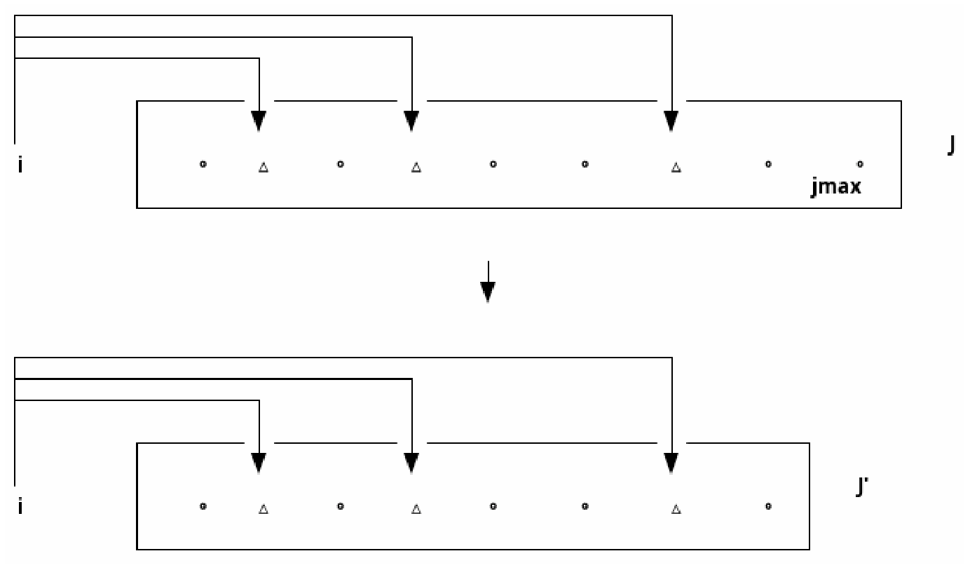
While the CA constraints ensure the user optimal principle under normal conditions (i.e., each customer is assigned to the closest available facility), MLCA extends this principle to handle scenarios where facilities are subject to failure or busyness, etc. The multi-level closest assignment principle is shown in Figure 1, where circles represent candidate sites for facilities, and triangles represent selected facilities. The facility sites (selected or not) are sorted by their distances to a given customer $i$. If the closest facility to $i$ becomes unavailable for any reason, customer $i$ must be assigned to its second closest, and if the second closest facility fails, $i$ must be assigned to the third closest and so on.

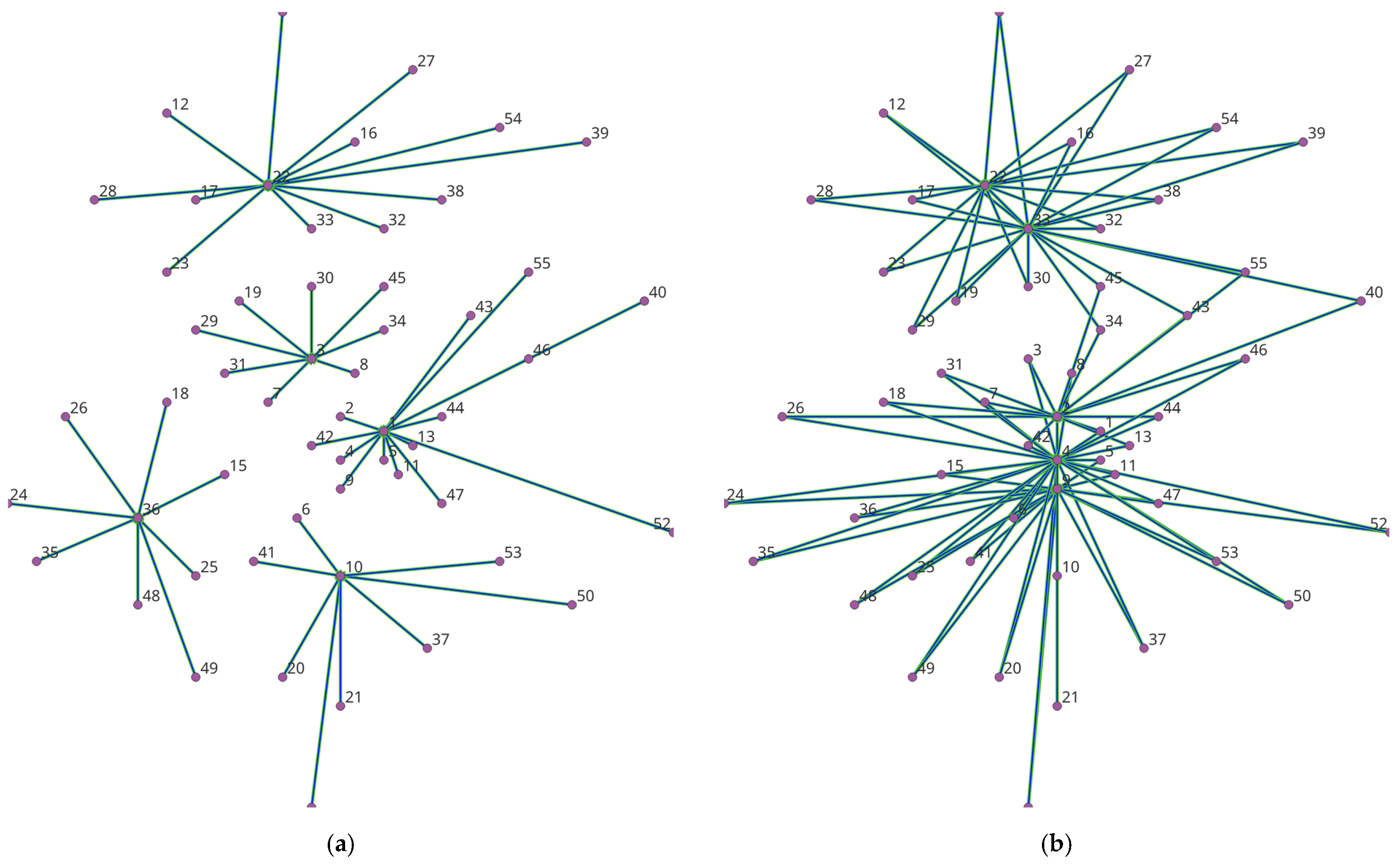
Weaver and Church [4] were the first to recognize the need to write explicit MLCA constraints when they created the vector assignment p-median problem (VAPMP), which was one of the first location-allocation models to recognize the need to redirect users to backup facilities. They proposed a form of MLCA constraint that generalizes a CA constraint form based on Rojeski and ReVelle [8]. Figure 2 illustrates an application of the MLCA constraints in the VAPMP on the Swain 55 node dataset widely used in GIS location modeling. The 55 points in the Figure represent customer locations (centroids of ZIP code zones in Baltimore, MD). Figure 2a presents the solution of the classic p-median problem with $p=5$ facilities (1, 3, 10, 22, and 36). This solution is optimal and minimizes total customer travel. By contrast, Figure 2b presents the solution of the VAPMP with failure probabilities (70% in this example). The effect of the MLCA condition is clear from this figure. Each customer is assigned to two facilities: a primary and a backup facility. The underlying assumption is that when the primary facility fails, the customer will go to the second closest facility. Consequently, the optimal solution shows a “pooling” pattern where the optimal facility locations form two tight clusters at 2, 4, and 9 and at 22 and 33, respectively. This is a reasonable location strategy because in a reliable location context, having backup facilities nearby lowers the potential travel cost when the primary facility fails (or becomes unavailable). The MLCA condition ensures that the location model can properly hedge against failures in making the location decision. While Figure 2 demonstrates how the MLCA constraint can be used to handle random failures in the VAPMP model, the MLCA can certainly be used in other reliable facility location models. For example, in a service system where the maximum travel time is important (e.g., express delivery and cold chain logistics), a reliable p-center problem [9] is defined to minimize the system’s worst case performance. The MLCA constraint can be used to enforce the closeness order in the reliable p-center problem just as in the VAPMP. The only difference is that the objective function is changed. A more expressive model generalizing both the reliable p-center problem and the VAPMP is presented in [13], in which the MLCA constraint is used in the same way.

However, as Weaver and Church correctly pointed out, the MLCA constraint is not required when the assignment vector is non-increasing, which is true in all their test data. Therefore, their MLCA constraint is untested. As pointed out in [3] and will be shown later on, the generalization of the Rojeski-ReVelle constraint in [4] is actually incomplete and missing a term. This incidence demonstrates the importance of rigorous proofs for analysts and users of ILP.

2.2. Theorem Proving for ILP

Logical conditions such as the CA constraints could be expressed using linear expressions. For example, given two binary variables $y_1$ and $y_2$, the linear inequality $y_1+y_2\le 1$ expresses the condition that, at most, one of the two variables can be one. For a set of $n$ binary variables $y_1,y_2,\dots ,y_n$, the linear inequality ${\displaystyle {\sum }_{i=1}^n}{y}_i\le p$ expresses the condition that, at most, $p$ of the $n$ variables can be one. Such linear expressions have been routinely used in formulating spatial optimization problems such as the p-median. With additional notation about sets and objects, the closest assignment condition can be expressed as linear constraints with a slightly more complex form (see, e.g., [3,12]).

One can see from the above integer-linear expressions the discrepancy between natural language logic (with logical connectives, conditional statements, etc.) and the linear expressions required in ILP formulations. In the examples above, the linear expressions are simple enough, and their meaning in natural language is quite clear. In more complex cases, the meaning of the linear expressions in ILP is not as obvious. It may require unraveling definitions and inferences in combination with other parts of the ILP model to extract the meaning of model constructs and establish the correctness of the model constructs (i.e., that the model property indeed holds).

Simple properties about ILP models can be established by mechanized proofs using modern proof assistants. Ref. [6] demonstrated how the correctness of the CA constraints can be proven using the Lean 4 proof language. As shown in [6], the primary advantage of using a computerized proof assistant is the rigor and completeness of the proof. Every proposition from the preliminary lemmas to the final theorem is derived from first principles and therefore is unmistakable. Proof languages that are based on dependent type theory (e.g., Lean 4) have the additional advantage of minimizing the set of axioms that are assumed to be true. In contrast, manual informal proofs can be incomplete and subject to human errors.

Even though ref. [6] demonstrated the feasibility of proving the correctness of (single-level) CA constraints, the proof techniques therein are relatively simple and cannot be applied to the multi-level version of CA constraints. Fundamentally, this is because the MLCA constraints involve multiple layers of intertwined decision variables (i.e., assignment variables), for which the correctness needs to be proven. By contrast, the CA constraint has only one layer of assignment variables. This means that one cannot prove the MLCA constraints by simply expanding definitions, substituting expressions, and simplifying terms, as in the CA proof in [6]. Instead, one has to repeatedly reduce the multi-layer MLCA proof problem into a smaller proof with one layer fewer assignment variables until there is no further reduction possible (i.e., the base case is reached). This process is known as a proof by induction (or recursion in programming).

Proof by induction for mathematical programs can be done informally using paper and pencil. However, it is more reliable to use a computerized proof assistant to establish the proof, as it is failsafe and unambiguous. In principle, any proof assistant that supports dependent type theory is suitable for the induction proofs of this article because of the Curry–Howard isomorphism between proofs and programs. The Curry–Howard isomorphism equates properties with types and proofs of a property with (functional) programs of the particular type (also known as terms). Consequently, proofs are also known as proof terms in type theory based proof languages. In such languages, proof by induction is essentially the same as a recursive program that repeatedly builds larger and larger proof terms from simple base case proofs. For example, given a property P defined on the natural numbers ℕ, a proof of mathematical induction corresponds to a recursive program of the following type using Lean 4’s syntax:

def P (n : ℕ) : Prop := n > 0

theorem P_true : P 0 → (P k → P (k + 1)) → (P n) := by sorry

Above, the property P is defined as a function from the natural numbers ℕ to the proposition type Prop. In Lean, t : T is the typing annotation, indicating that t is of type T. The application of a function f to a value x is written succinctly as f x. So, P n is the application of P to the natural number n (or the property that P is true for n). The second “:” in the definition def P (n : ℕ) : Prop indicates that P n is a property (i.e., is of type Prop) that we want to prove. In general, the term after the top-level “:” is the return type of a function (or conclusion of a theorem). The assignment operator := is used to assign a value of the right type to the name P. Here, we just use a simple proposition n > 0 as the value.

The theorem P_true is a proof of mathematical induction. It states that if P is true for the base case (i.e., P 0), and if for each k, P k implies P (k + 1), then P is true for any n : ℕ. Note that the arrow symbol → is used to express the function type. In general, t1 → t2 → … → tn → r is the type of an n-ary function that takes n parameters of the types t1, …, tn and returns a value of type r. In the type signature of P_true, (P k → P (k + 1)) is itself a function type transforming a (smaller) proof term for P k to a (bigger) term P (k + 1). This transformation is commonly known as the induction step in regular mathematical language. Interestingly, by Curry–Howard isomorphism, the principle of induction proofs is now reduced to the construction and use of normal recursive functions of the type (P k → P (k + 1)), i.e., the induction step(s). Then, the recursive function is applied repeatedly in the example to construct proofs of larger and larger n until we get to all n in ℕ.

In the example, we omit the actual body of P_true and just use the term sorry, which is a placeholder term indicating the actual content is omitted, and one just assumes that there exists a suitable term at this position. It should be replaced with legitimate terms eventually when the proof is completed. For this particular example, P n cannot be true for all n because there exists no evidence for P 0 (i.e., 0 > 0). In other words, the type P 0 is empty. But the induction principle P_true is still true. If we had an evidence h0 : 0 > 0 and a valid induction step function f : P k → P (k + 1), then we could construct a proof P n for any n.

In principle, one could construct proof terms for a theorem directly. If one knows of a theorem of the type th : t1 → t2 → … → tn → r and evidence of each prerequisite assumption h_i : ti, then one can simply apply the theorem to the assumptions (or hypotheses), just as if applying a function to the input values. And the result term th t1 t2 … tn : r is an evidence of r as needed. When the proofs of the assumptions are not yet all known, one can use an underscore _ as a placeholder to construct a partial proof of the goal. This placeholder can then be refined in place by replacing it with a term of the right type. If the refinement process ends with a concrete term with no holes, a proof of the original theorem is found. This process is known as type-driven development (TDD) [14] and languages such as Idris2 provide built-in support for it. Without built-in support, one can still inspect the types of holes and manually supply the proof terms. Generally, directly constructing proof terms like this requires expertise and intimate knowledge of the theorems (and inductive definitions) of a domain. A large portion of proofs in the Lean standard library are indeed provided as direct proof terms.

As an alternative to direct term construction, one can also use a set of commands called “tactics” in Lean (and similar languages such as Coq) to help construct proof terms. For example, one can use the apply command to partially apply a theorem by matching its conclusion with the current goal and making any unfulfilled assumptions of the theorem new sub-goals to be proven later on. The rw tactic is used to rewrite equivalent terms at any level of tree of proof terms according to an equality. While theoretically, one could use these tactics to construct all proof terms, additional tactics are frequently used to facilitate case analysis, induction, and so on. The reader is referred to the Lean documentation [15] for a comprehensive list of the tactics and Lean language features.

In the next section, we use the Lean 4 proof language to prove the correctness of the MLCA constraints. We demonstrate the feasibility of proving such complex properties using a combination of basic lemmas about integer-linear expressions and customized induction principles. This establishes a rigorous proof of the specific MLCA, which has not been previously presented in the literature. We also discuss the engineering issues of building the proof along the way.

3. Method

In this section, we present the integer linear programming formulation of the MLCA condition and the translation of its correctness condition into logic and demonstrate how it can be proven in a series of lemmas and theorems using type theory-based languages such as Lean 4. In particular, we show how custom induction principles can be used to solve complex proof problems involving multiple layers of interdependent decision variables.

3.1. Formulation of MLCA Constraints

There are multiple ways to formulate the closest assignment [12] and the multi-level closest assignment constraints [3]. The following common notation is needed:

$I$, $J$ are the sets of customer locations and potential facility sites, and $i$, $j$ are the corresponding indices representing customer and facility locations, respectively.

$L$ is the maximum number of levels of closest assignment considered in the location model, and $l=\mathrm{0,1},2,\dots \left(L-1\right)$ is an index representing the level of closest assignment (i.e., the assignment of customers to the $l^{th}$ closest facility.

$d_{ij}$ is the distance between locations $i$ and $j$.

$C_{ij}=\{q\in J|d_{iq}<d_{ij} \mathrm{or} d_{iq}=d_{ij} \mathrm{when} q<j\}$ is the set of candidate sites that are closer to a customer $i$ than site $j$. When there is a distance tie to $i$, facilities with lower site indexes are considered to be closer (to break the tie). We call $C_{ij}$ the closeness sets. Collectively, the nested collection of sets $C_{i\cdot }$ characterizes the order of closeness of candidate sites for a given customer location $i$, where the closeness set $C_{i{j}_1}$ for a closer site $j_1$ is the subset of the closeness sets $C_{i_{j_2}}$ for a more distant site $j_2$. Note that it is important to break the distance tie, as it ensures that the nested structure of the closeness sets is well-defined, and the Lean proof relies on the uniqueness of this closeness ordering for the induction proofs in this article to hold.

The relevant decision variables are

$$y_j=\{\begin{array}{c}1, \mathrm{if} \mathrm{candidate} \mathrm{site} j \mathrm{is} \mathrm{selected} \mathrm{as} \mathrm{a} \mathrm{facility}\\ 0, \mathrm{otherwise}\end{array}$$

(1)

$$x_{ij}^l=\{\begin{array}{c}1,\hspace{0.25em}\mathrm{if} \mathrm{site} j \mathrm{houses} \mathrm{the} l^{th} \mathrm{closest} \mathrm{facility} \mathrm{for} \mathrm{customer} i\\ 0, \mathrm{otherwise}\end{array}$$

(2)

when only the closest facility is considered (i.e., $L=1$), we abbreviate $x_{ij}^0$ as $x_{ij}$.

In this article, we only study one of the several forms of the MLCA constraints, which is an extension of the single-level CA constraint first proposed by Rojeski and ReVelle [8] in studying a budget-constrained p-median problem. We chose this form because it is the earliest and one of the most efficient formulations in the single-level and multi-level forms [3,12]. The constraint set is as follows:

$$x_{ij}\ge y_j-\sum _{q\in C_{ij}}{y}_q \forall i\in I,j\in J$$

(3)

$$\sum _{j\in J}{x}_{ij}=1, \forall i\in I$$

(4)

The modeling construct in Constraints (3) and (4) is not a complete ILP program, for it has no objective function, and other constraints are needed to describe a full model. However, this construct alone is sufficient to enforce the closest assignment condition and therefore can be used in any model that requires the closest assignment. More specifically, (3) maintains that for each candidate site $j$ ($\forall j,\cdots$), if a site $j$ is selected as a facility (i.e., $y_j=1$), and no other site closer to $i$ than $j$ is selected (i.e., $\sum _{q\in C_{ij}}{y}_q=0$), then $x_{ij}$ is forced to be one. When $j$ is not the closest facility (i.e., $\sum _{q\in C_{ij}}{y}_q\ge 1$), the constraint (3) is non-binding. The constraint (4) is the assignment constraint maintaining that for each customer $i$, if it is assigned to a facility $j$ ($x_{ij}=1$), it cannot be assigned to any other facility in $J$, i.e., one must have $x_{i{j}^{\prime }}=0$ for all $j^{\prime }\ne j$.

Ref. [3] generalizes the CA constraints above into the following multi-level form:

$$x_{ij}^l\ge y_j-\sum _{q\in C_{ij}}{y}_q+\sum _{s<l}\sum _{q\in C_{ij}}{x}_{iq}^s-\sum _{s<l}{x}_{ij}^s, \forall i\in I,j\in J, \mathrm{and} l=\mathrm{0,1},2,\dots ,L-1$$

(5)

$$\sum _{j\in J}{x}_{ij}^l\le 1, \forall i\in I,\hspace{0.25em}l=\mathrm{0,1},\dots ,\left(L-1\right)\hspace{0.25em}$$

(6)

$${\displaystyle \sum _{l=1}^L}{x}_{ij}^l\le 1 \forall i\in I,j\in J$$

(7)

Informally, constraint (5) is a generalization of the Rojeski-ReVelle CA constraint (3). It forces the assignment variable $x_{ij}^l$ at level $l$ to be one when (i) $j$ is a facility, (ii) all facilities closer than $j$ ($\sum _{q\in C_{ij}}{y}_q$) are matched by lower level assignments elsewhere ($\sum _{s<l}\sum _{q\in C_{ij}}{x}_{iq}^s$), and (iii) $i$ is not assigned to $j$ at a lower level than $l$ (i.e., $\sum _{s<l}{x}_{ij}^s=0$).

Constraint (6) maintains that at each closeness level $l$, each customer $i$ can be assigned to at most one facility. It is a generalization of the assignment constraint (4) to multiple levels. Constraint (7) maintains that each customer $i$ can be assigned to some facility $j$ for at most one closeness order $l$ (i.e., a given site $j$ cannot be both the $l^{th}$ and the $s^{th}$ closest facility for $l\ne s$).

It should be noted that in the original paper for the vector assignment p-median problem (VAPMP) [4], a form of the generalized Rojeski-ReVelle constraint similar to (5), has been presented, with only a short verbal justification for why it would work. However, the constraint form in [4] is incomplete, and the last term in (5) (i.e., $-\sum _{s<l}{x}_{ij}^s$) is missing. Presumably, this is because the MLCA constraint is not needed when the assignment vector in VAPMP is not non-decreasing [4]. Therefore, this use case was never tested in [4], and this omission was never detected until a later article by [3]. The incomplete form of the MLCA is infeasible in the sense that if one views the MLCA condition as an optimizer model with a trivial objective function 0, the model has no feasible solution. Consequently, if the incomplete form is used in a model, it will make the entire model infeasible. This incidence shows how important it is to rigorously prove the correctness of ILP constructs.

3.2. Correctness of the Closest Assignment Constraints

Given an ILP model or modeling construct, a natural question is the following: what does it mean for it to be correct? An ILP modeling construct is correct if the optimal solution (and the associated values of the decision variables) have the intended property. In the case of (multi-level) CA constraints, an objective function is neither required nor present. One only needs to show that if a solution ($x_{ij}^l$ and $y_j$) meets all the relevant constraints, the logical condition in their definition (i.e., the intended meaning) in definition (2) must hold. That is, if $j$ is the $l^{th}$ closest facility to customer $i$, then one must have $x_{ij}^l=1$, and for all $s\ne l$, one must have $x_{ij}^s=0$. If this can be proven, then any objective function value based on the assignment variable $x_{ij}^l$ would correctly count various distances $d_{ij}$ associated with the non-zero assignments $x_{ij}^l$.

As mentioned earlier, informal proofs or verification by test cases can be incomplete or error-prone. Therefore, we explore a precise computerized proof of the correctness of the MLCA constraint (5) in this article. Such computerized proof rules out many possible errors and ambiguities. Using the closeness set $C_{ij}$, we can precisely express the logical condition “$j$ is the $l^{th}$ closest facility to customer $i$” with a linear expression $\sum _{q\in C_{ij}}{y}_q=l$. In Lean4, this is written as

∑ q ∈ C_i J d j, y q = l

It can be observed that the above lean code looks the same as a logical formula in ILP, except that (i) the formula is flattened into a computer format that is “executable”, and (ii) the closeness set $C_{ij}$ is written with full information including the distance matrix $d$ and the candidate site/set etc. Likewise, given appropriately defined values of $x,y,i,j,l$, the correctness of the CA constraint can be written in Lean4 as follows (assuming the constraint (5) is satisfied):

y j = 1 → (∑ q ∈ C_i J d j, y q = l) → x j l = 1

Similarly, ref. [6] presented a computerized proof of the single-level Rojeski-ReVelle CA constraint (3) in the context of the p-median problem. The proof is relatively simple. It involves the expansion of definitions and simplification of equations and inequalities. In the Lean proof language, the correctness of (3) boils down to the following logical implication (which is a special case of the multi-level version above):

y j = 1 → (∑ q ∈ C_i J d j, y q = 0) → x i j 0 = 1

The two assumptions, y j = 1 and ∑ q ∈ C_i J d j, y q = 0, are two equations. One can substitute them (using the rw tactic) into the CA constraint (3) to obtain

x i j 0 ≥ 1 – 0

Combining this fact with the definition of x i j 0 (that it is between 0 and 1), we have x i j 0 = 1. Using term rewriting and simplification and applying standard theorems in the Lean’s mathlib library, ref. [6] proved the single-level CA constraint (in addition to other properties of the p-median problem). However, such simple proof techniques are insufficient for the proof of the multi-level CA constraints. For example, if one tries to rewrite the more general assumption ∑ q ∈ C_i J d j, y q = l into the MLCA constraint (5), one obtains the following:

$x_{ij}^l\ge y_j-l+\dots -\dots$, without knowing what the value of $l$ is. Consequently, one cannot directly simplify this into $x_{ij}^l\ge 1$ as before. Instead, one needs to know the value of $x_{ij}^{l-1}$, the value of $x_{ij}^{l-2}$, and so on before proving anything about $x_{ij}^l$.

The general idea of proving more complex properties such as the MLCA correctness is to use induction. The gist is that if one knows that the fact that the property in question is true for all lower values of $l^{\prime }$ (than $l$), and it implies that the property is true for $l$, then the property must be true for all $l$. This means that the original proof is reduced to a sequence of smaller proofs until the proof cannot be any smaller (e.g., when $l$ reaches 0).

Of course, the properties of an ILP model are more complex to express than the properties of simple natural numbers and require complex data structures (such as the nested sets $C_{ij}$). The induction principles are also more complex and involve reducing bigger data structures into smaller ones until base case(s) are reached. In the next subsection, we present the necessary definition and data structure for the induction proof in Lean.

3.3. Basic Definitions

To facilitate the induction proof of MLCA construct, we collect all necessary definitions of variables and related constraints into one Lean4 structure called VAModel_i to represent the vector assignment model for customer $i$, as shown below. Note again that this is not a complete ILP model such as VAPMP or OSEM. Instead, it is just the relevant segment of an ILP model characterizing the MLCA conditions. Note also that the partial model is written for a fixed customer $i$. This is because the order of closeness of facilities in $J$ changes from one customer to another. Therefore, the order of induction (or recursion) also changes, and we have to fix the customer $i$ in the proof.

structure VAModel_i [LinearOrder α] (I J: Finset α)

(d: α → ℚ)

(i : α) (imem : i ∈ I)

(L :ℕ)

where

(x: α → ℕ → ℚ)

(y : α → ℚ)

(xDef: ∀ j ∈ J, ∀ l ∈ Finset.range L, 0 ≤ x j l ∧ x j l ≤ 1)

(yDef : ∀ j ∈ J, binary (y j))

(cLevel: ∀ j ∈ J, (∑ l ∈ Finset.range L, x j l) ≤ 1)

(cLevel2: ∀ l ∈ Finset.range L, (∑ j ∈ J, x j l) ≤ 1)

(cCA: ∀ j ∈ J, ∀ l ∈ Finset.range L,

x j l + ∑ q ∈ C_i J d j, y q + ∑ s ∈ Finset.range (l), x j s

≥ y j + ∑ s ∈ Finset.range (l), (∑ q ∈ C_i J d j, x q s))

The definition above is similar to the Lean4 definition of the classic p-median problem in [6]. Lean4 uses square brackets to express the so-called typeclass constraints and curly braces ({}) to express implicit arguments. The reader is referred to the Lean4 documentation for details and to [6] some example usages of these Lean4 syntax in the context of ILP. The essential definition of the MLCA conditions includes the following: α is the type of various indices or IDs (for customers and facility locations). For example, it can be the type of integers or text strings. Generally, we only require α to be a linearly ordered type (LinearOrder) so that we can compare indices. I, J are finite sets (Finset) of IDs for the customers and candidate sites, respectively. d: α → ℚ is the slice of distance matrix for customer $i$. In other words, it is a function or array from each facility index $j$ to a rational number (ℚ) representing the distance $d_{ij}$. (i : α) is the customer $i$ for which the vector assignment model is written, and (imem : i ∈ I) is a proof that i is a member of the index set $I$ (i.e., $i$ is a valid index). The constants before the where command are literal translations of the ILP definitions into the proof language.

Below the where command are the essential definitions based on the constants. (x: α → ℕ → ℚ) is the decision variable $x_{ij}^l$ for a fixed $i$. In Lean4, it is defined as a function/array from (j: α) and a natural number (l : ℕ) to the value of $x_{ij}^l$ in ℚ. Similarly, the location variable $y_j$ is defined as an array on the index type α. In the rest of this article, we use the variable m or m’ in Lean4 to represent a vector assignment model (or VA model) for customer $i$. And we write m.x j l for the variable $x_{ij}^l$ in this VA model, m.y j for the variable $y_j$, and so on. Note that the customer index $i$ is included as part of the vector assignment model.

With this in mind, m.xDef defines for each $l<L,j\in J$ the domain of the variable m.x j l to be $\left[\mathrm{0,1}\right]$. m.yDef defines $y_j$ to be binary variables. m.cLevel and m.cLevel2 express the two level constraints (6) and (7). m.cCA is the generalized Rojeski-ReVelle constraint (5) translated into Lean4. After bundling all necessary information into the VAModel_i structure, the main theorem of this article can be expressed using a model variable (m : VAModel_i I J d i imem L) as follows:

theorem mlca_rr1_correct [LinearOrder α] (I: Finset α)

(d : α → ℚ)

(i : α) (imem : i ∈ I)

(J: Finset α)

: ∀ (L :ℕ) (m : VAModel_i I J d i imem L)

(l:ℕ) (lmem: l ∈ Finset.range (L)) (j:α) (jmem:j ∈ J),

m.y j = 1 → (∑ q ∈ C_i J d j, m.y q = l) → m.x j l = 1

Note that we only prove m.x j l = 1 in the conclusion of the main theorem. The other part of the conclusion ∀ s ∈ Finset.range L, s ≠ l → m.x j s = 0 is an easy consequence of the level constraint (6) and is proven in a corollary of the main theorem.

A data type that is extensively used is the finite set of elements of α, written as Finset α in Lean 4. The main purpose of using Finset α in ILP proofs is to replace intervals of natural numbers as index sets. Traditionally, index sets such as $I$ are often defined as intervals such as $I=\mathrm{1,2},\dots m$ (called ranges in Lean 4). This is fine for many applications of ILP, but in theorem proving and induction, we may need to work recursively on subsets of $I$, which are generally not contiguous intervals of numbers. Therefore, we need a different data structure. We use a type parameter α in Finset α just to allow other types such as text strings to be used as index sets. Of course, we occasionally use ranges of natural numbers, e.g., to represent the closeness level $l=\mathrm{0,1},\dots ,L-1$. In Lean4, this is written as Finset.range L.

Mathematically, we need the finite Finset instead of an arbitrary set so that summations can be written. If the set in question is infinite, its sum may not be well-defined. We have already used such summations in defining the closeness set ∑ q ∈ C_i J d j = 0. Throughout the proof of the MLCA constraint, we use many theorems about Finset. For example, given a logical condition $p$, a finite index set $s$, and a list of mixed values chosen conditionally from two arrays a, b, we can split the sum into two sums for each array based on whether p holds:

$$\sum _{i\in s} \mathrm{if} p\left(i\right) \mathrm{then} a\left(i\right) \mathrm{else} b\left(i\right)=\sum _{i\in s\wedge p\left(i\right)}a\left(i\right)+\sum _{i\in s\wedge p̸\left(i\right)}b\left(i\right)$$

In Lean4, this is written as follows:

Finset.sum_ite {ι} {M} [AddCommMonoid M] {s : Finset ι} {p : ι → Prop} [DecidablePred p]

( a b : ι → M) : (∑ i ∈ s, if p i then a i else b i) = ∑ i ∈ s with p i, a i + ∑ i ∈ s with ¬p i, b i

Another theorem Finset.sum_nonneg states that if every element of an array is non-negative, then the sum of this array is non-negative. Simple as they are, these basic theorems/lemmas constitute the bulk of the proof about the ILP constructs of this article.

3.4. Induction

From the perspective of proof theory, proof by induction is in essence a recursive function from the proofs of the base cases and inductive steps to the proof of the theorem in question. As mentioned earlier, mathematical induction is a function from $P\left(0\right)$ and $\forall k,P\left(k\right)\to P\left(k+1\right)$ to $\forall n,P\left(n\right)$. There are two ways to view the principle of mathematical induction. First, from a bottom-up point of view, the principle tells us that if we have a proof for $P\left(0\right)$ and a step function from $P\left(k\right)$ to $P\left(k+1\right)$, then we can construct proofs of $P\left(1\right)$ (from $P\left(0\right)$), $P\left(2\right)$ (from $P\left(1\right)$), $P\left(3\right)$, …, all the way to $P\left(n\right)$ for any natural number $n$. Second, from a top-down point of view (and in terms of proof obligations), the induction principle tells us that to prove $P\left(n\right)$, we just need to prove $P\left(n-1\right)$ (by the induction step); for $P\left(n-1\right)$, we just need to prove $P\left(n-2\right)$, $P\left(n-3\right)$, … until we reach the base case, in which we just need to prove $P\left(0\right)$. We know that this descending chain of natural numbers must end in a finite number of steps; therefore, this recursive process must terminate.

The proof of the MLCA requires a more fine-grained control of the recursive process and a more complex induction principle for the finite sets, expressed in Lean4 as the following theorem:

Finset.induction_on_max_value {α} {ι} [LinearOrder α] [DecidableEq ι] (f : ι → α)

{p : Finset ι → Prop} (s : Finset ι) (h0 : p ∅)

(step : ∀ (a : ι) (s : Finset ι), a ∉ s → (∀ x ∈ s, f x ≤ f a) → p s → p (insert a s)) : p s

In this theorem, s : Finset ι is a finite set. f is a measure function on the index type ι, p is the property to be proved about the finite set, and h0 : p ∅ is the base case (that p is true on empty set). The induction step step : ∀ (a : ι) (s : Finset ι), a ∉ s → (∀ x ∈ s, f x ≤ f a) → p s → p (insert a s) states that for every s and an outside element a ∉ s that is greater than all of s (by the measure f), one can construct a proof that the property also holds for $s\cup \left\{a\right\}$ (written as insert a s in Lean4). Then, the conclusion of the theorem … : p s states that p holds for any finite set s. 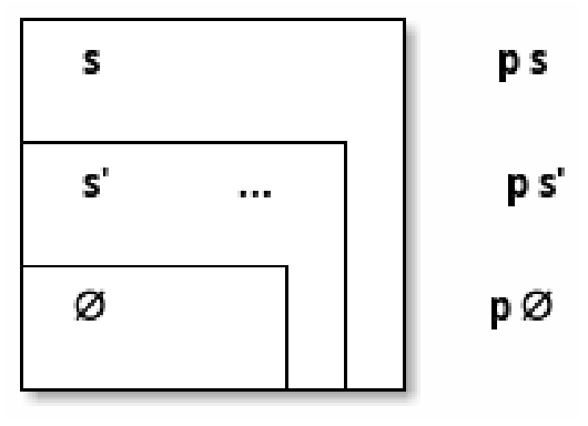Figure 3 depicts the recursive structure of the induction proof.

From a top–down point of view, the induction principle in Figure 3 can also be interpreted as backward reasoning. To prove that p is true for a finite set s, it is necessary to prove that p is true for $s\backslash \left\{a_{max}\right\}$ (i.e., set s minus its maximal element a_max with respect to measure f). And if one has a general way to prove this induction step, then one only needs to prove $p$ for smaller and smaller versions of s, and all that is left is to prove the base case when s = ∅.

The main idea behind the proof of the MLCA constraints is to perform induction on the set of candidate sites $J$ using the above induction principle. In each step, we shrink the current candidate set by erasing from it the greatest element $j_{max}$ in terms of the distance to the fixed customer $i$. Then, both the candidate sites $J$ and the closeness set $C_{ij}$ are smaller by one element ($j_{max}$). As shown in Figure 4, the proof goal is restored to the same format as the original goal, i.e., MLCA is correct on the smaller data $J^{\prime }$, ${C^{\prime }}_{ij}$. The induction step, as a sub-goal, is that the correctness on the smaller data implies the correctness on the current data.

How does one use such a complex induction principle in Lean4 proofs? A primitive way is to recall that an induction principle in Lean4 is just a regular theorem, and one can use the apply command on it. Then, Lean4 will reduce the proof of the conclusion to the proofs of the premises (here, the base cases and induction hypotheses), as shown in the code snippet below:

apply Finset.induction_on_max_value (fun j => (d j, j))

(p := fun J =>

∀ (L :ℕ) (m : VAModel_i I J d  i imem L)

(l:ℕ) (lmem: l ∈ Finset.range (L)) (j:α) (jmem:j ∈ J),

m.y j = 1 → (∑ q ∈ C_i J d j, m.y q = l) → m.x j l = 1

) J

. -- base case

show ∀ (L : ℕ) (m : VAModel_i I ∅ d i imem L), ∀ l ∈ Finset.range L,

∀ j ∈ ∅, m.y j = 1 → ∑ q ∈ C_i ∅ d j, m.y q = ↑l → m.x j l = 1

simp

· -- inductive step

show ∀ (a : α) (s : Finset α),  a ∉ s → (∀ x ∈ s, (d x, x) ≤ (d a, a)) →

(∀ (L : ℕ) (m : VAModel_i I s d i imem L),

∀ l ∈ Finset.range L, ∀ j ∈ s, m.y j = 1 → ∑ q ∈ C_i s d j, m.y q = ↑l → m.x j l = 1) →

∀ (L : ℕ) (m : VAModel_i I (insert a s) d i imem L),

∀ l ∈ Finset.range L, ∀ j ∈ insert a s, m.y j = 1 → ∑ q ∈ C_i (insert a s) d j, m.y q = ↑l → m.x j l = 1

sorry

In the above application of Finset.induction_on_max_value, the first argument fun j => (d j, j) is the measure function needed to define the maximal element $j_{max}$. In particular, it is a lexicographic order based on the distance to customer $i$ and then on the order of the site indices. The second argument (p := fun J => ∀ (L :ℕ) …, m.y j = 1 → (∑ q ∈ C_i J d j, m.y q = l) → m.x j l = 1) is the correctness of the MLCA constraint (5) in Lean4. The third argument J is the finite set on which we are performing the induction. The two subsequent dot (.) commands represent the two sub-goals that are generated after applying the induction principle. The first sub-goal is the base case in which $J$ is ∅. We spelled out the sub-goal using the optional show command (which does nothing except for serving as a comment). One of the presumptions ∀ j ∈ ∅ is impossible. Therefore, the base case holds vacuously. In Lean 4, the simplification command (simp) can detect such impossible assumptions and close the current (sub)goal.

The second sub-goal is the induction step and is more complex; we only show its statement and use the sorry command to omit its proof for now. In the statement, the upward arrow in ↑l represents an automatic type conversion of l (from ℕ to ℚ). The statement is long, but it is just a verbatim translation of the induction step, asserting that one can construct the bigger proof for p (insert a s) from the smaller proof p s. Compared with Figure 4, (insert an s) is the bigger set $J$ and s is the smaller set $J^{\prime }$. They differ by one element a, which corresponds to the maximal element $j_{max}$ in Figure 4.

We also used specialized induction principles to prove useful properties about binary variables. For example, we need theorems about the sum (∑) of binary variables. If the sum of the $y_j$ variables in the closeness set is $c$ (∑ q ∈ C_i J d j, m.y q = c), we know that there exist exactly $c$ sites in $C_{ij}$ for which the $y_j$ value is one and vice versa. This is described by the following theorem and proven using a different induction principle Finset.induction_on. (Note that s.card is the cardinality/size of set s.)

theorem ex_array_of_binary_sum [LinearOrder α] {I0: Finset α}

{I: Finset α} (hI: I ⊆ I0) {y : α → ℚ} (hbin : ∀ i ∈ I0, binary (y i))

: ∀ (c : ℕ),  ∑ i ∈ I, y i = c → ∃ I′, I′ ⊆ I ∧ I′.card = c ∧

(∀ i ∈ I′, y i = 1) ∧ (∀ i ∈ I \ I′, y i = 0)

3.5. Auxiliary Definitions and Theorems

We also list some of the auxiliary theorems and definitions that we found useful for writing our ILP proofs. The theorem below states that, for an array f of binary variables, if its sum is less than or equal to one, then only one element can be one. This lemma expresses the exclusiveness of binary values if they add up to one. If we already know one i for which f i is one, then the rest of the array elements must be zero. We use this lemma (among other things) to prove the corollary of the main theorem using the level constraint (6) for the exclusiveness condition.

theorem zero_elsewhere_of_sum_one [LinearOrder α] {I: Finset α}

{f : α → ℚ} (hnonneg : ∀ i ∈ I, f i ≥ 0) (i : α)

(imem : i ∈ I) (hfi: f i = 1) (hsum: ∑ i ∈ I, f i ≤ 1)

: ∀ i′ ∈ I, i′ ≠ i → f i′ = 0

An important definition is the shrunken version of the candidate set $J$ in Figure 4. We constructively define the bigger, original version of the candidate site in induction as insert jmax J, where insert is the basic operator to insert an element into a finite set to create a bigger set. We then use J to represent the smaller version of the candidate set. The other inputs state the conditions that jmax is outside of J (jmax_nmem), is a maximal element (jmax_max), and so on. This pattern of bigger/smaller sets matches the specific induction principle Finset.induction_on_max_value discussed earlier. Overall, the function model_erase_fac returns a smaller version of $J\cup j_{max}$ in which $j_{max}$ is removed.

def model_erase_fac [LinearOrder α] (I J: Finset α)

(d: α → ℚ) (L : ℕ) (i : α) (imem : i ∈ I)

(jmax : α) (jmax_nmem : jmax ∉ J) (jmax_max : ∀ j ∈ J, (d j, j) ≤ (d jmax, jmax))

(m : VAModel_i I (insert jmax J) d  i imem L)

: VAModel_i I J d i imem L

where

x := m.x

y := m.y

xDef := by

intro j jmem

exact m.xDef j (Finset.mem_insert_of_mem jmem)

-- …

The return value of model_erase_fac is the shrunken version of the original model m. Call this new model m’. Its fields are defined in the where clause in terms of the original model m. In the where clause, the line x := m.x means that the x variable in the new model m’ is defined to be the same α → ℕ → ℚ function as the original model, except that its domain in α is smaller (J instead of insert jmax J). In other words, m’.x as a function is the restriction of m.x on J.

The restriction of the domain is reflected in the new definition of $x_{ij}^l$ in m’.xDef, which has the type ∀ j ∈ J, ∀ l ∈ Finset.range L, 0 ≤ m.x j l ∧ m.x j l ≤ 1. The goal still states that m’.x is between 0 and 1, but the domain changes, and we only need to prove the goal for j ∈ J. Since J is a subset of insert jmax J, the evidence jmem : j ∈ J can be transformed into a new evidence that j ∈ insert jmax J using the theorem Finset.mem_insert_of_mem. This is why we use the term Finset.mem_insert_of_mem jmem : j ∈ insert jmax J as input to the original $x$ definition m.xDef, which gives us the desired property (that m’.x j l is also between 0 and 1). The remaining fields (omitted here) similarly define the smaller model m’ in terms of the original model m.

To prove the induction step, we need to establish a link between the bigger and smaller versions of model in Figure 4. In the lemma below, we show that the assignment variable $x_{ij}^l$ on the smaller model m’ has the same values as the bigger m after erasing the maximal element jmax. Intuitively, this is because removing the largest element in m does not change the order of assignments in the remaining part of m. The proof of this lemma is just a simplification after expanding the definition of model_erase_fac.

lemma model_erase_fac_x_eq [LinearOrder α] (I J: Finset α)

(d: α → ℚ) (L : ℕ) (i : α) (imem : i ∈ I)

(jmax : α) (jmax_nmem : jmax ∉ J) (jmax_max : ∀ j ∈ J, (d j, j) ≤ (d jmax, jmax))

(m : VAModel_i I (insert jmax J) d  i imem L)

: ∀ j ∈ J, ∀ l ∈ Finset.range (L),

(model_erase_fac I J d L i imem jmax jmax_nmem jmax_max m).x j l = m.x j l := by

simp [model_erase_fac]

We similarly establish in lemma model_erase_fac_y_eq the equality between the location variable $y_j$ of the original model and the erased model. Another set of useful lemmas connect the closeness set $C_{ij}$ before and after removing the maximal element $j_{max}$. The following lemma states that if one removes an element from $J$ that is greater than or equal to the bound $j$ of $C_{ij}$, the closeness set $C_{ij}$ remains the same.

theorem C_erase_ge_idem [LinearOrder α] {J: Finset α}

{d: α → ℚ} {jmax : α} {j:α} (hge: (d j, j) ≤ (d jmax, jmax))

: C_i (J.erase jmax) d j = C_i J d j := by sorry

Symmetrically, the lemma C_insert_ge_idem states that if one expands $J$ by an element jmax that is outside $J$ and greater than or equal to all elements of $J$, then the closeness set $C_{ij}$ remains the same. This lemma is an easy corollary of the previous lemma and is proven by a simple rewrite. The have hC_i := … line creates an instance of the theorem C_erase_ge_idem that is applied to insert jmax J. The rw [Finset.erase_insert jmax_nmem] at hC_i command uses the fact that insert and erase operations cancel out (Finset.erase_insert) and rewrite ((insert J jmax).erase jmax) into J in the hypothesis hC_i, which renders exactly the property we need.

theorem C_insert_ge_idem [LinearOrder α] {J: Finset α}	(8)
{d: α → ℚ} {jmax : α} (jmax_nmem : jmax ∉ J) {j:α} (hge: (d j, j) ≤ (d jmax, jmax))
: C_i (insert jmax J) d j  = C_i J d j := by
have hC_i := C_erase_ge_idem (J:=insert jmax J) (hge:=hge)
rw [Finset.erase_insert jmax_nmem] at hC_i
exact (Eq.symm hC_i)

One last example of lemmas about closeness sets is the following theorem, which states that if the bound of the closeness set is greater than or equal to all of J, then the closeness set is the whole J. In the lemmas presented here, we make many arguments implicit by declaring them in braces (e.g., {J: Finset α}) to ease their use for term rewriting because in rewriting, the target expression to rewrite (the conclusion) is already known, and the bits of information we made implicit can be inferred from the target.

theorem C_bound_ge [LinearOrder α] {J: Finset α}

{d: α → ℚ} {jmax : α} (jmax_nmem : jmax ∉ J) (jmax_max: ∀ j ∈ J, (d j, j) ≤ (d jmax, jmax))

: C_i J d jmax = J

3.6. Outline of the Main Proof

Using the basic definitions and auxiliary theorems introduced so far, we outline the major steps of the main theorem mlca_rr1_correct. For space reasons, we state the sub-goals at important points and omit most of the proofs of intermediate steps, which mostly consist of the application of stock theorems about Finset, the new lemmas described earlier, term rewriting, and simplification of proof states. The sub-goal for the base case p has already been proven. So, we focus on the second sub-goal, the induction step. We first simplify terms and fix universally quantified variables using the intro command:

simp [- Finset.mem_range]

intro jmax J′ jmax_nmem jmax_max ihs L m l lmem

We use simp [- Finset.mem_range] instead of simp to avoid using the simplification rule Finset.mem_range, which would convert l ∈ Finset.range L to l < L and therefore break some of the finite sums (∑ l ∈ Finset.range L, …). Now, we obtain the following proof state with assumptions above the turnstile sign ⊢ and the goal after it. We can observe that the simplification broke the previous goal …, ∀ j ∈ insert a s, m.y j = 1 → ∑ q ∈ C_i (insert a s) d j, m.y q = ↑l → m.x j l = 1 into a conjunction of two parts. This is because j ∈ insert a s is equivalent to a disjunction of two cases: ∀ j = a ∨ j ∈ s, each corresponding to a smaller sub-goal of the new goal. This is generally how we prove the theorems in this article: by reducing the current goal to simpler sub-goals that are easier to solve.

-- …

jmax : α

J′ : Finset α

jmax_nmem : jmax ∉ J′

jmax_max : ∀ x ∈ J′, (d x, x) ≤ (d jmax, jmax)

ihs : ∀ (L : ℕ) (m : VAModel_i I J′ d i imem L),

∀ l ∈ Finset.range L, ∀ j ∈ J′, m.y j = 1 → ∑ q ∈ C_i J′ d j, m.y q = ↑l → m.x j l = 1

L : ℕ

m : VAModel_i I (insert jmax J′) d i imem L

l : ℕ

lmem : l ∈ Finset.range L

⊢ (m.y jmax = 1 → ∑ q ∈ C_i (insert jmax J′) d jmax, m.y q = ↑l → m.x jmax l = 1) ∧

∀ a ∈ J′, m.y a = 1 → ∑ q ∈ C_i (insert jmax J′) d a, m.y q = ↑l → m.x a l = 1

Given the conjunction of sub-goals, we use the constructor command to break it into two sub-goals. But before that, we establish common definitions and facts shared by the two sub-goals. In particular, we use the set command to give a name m’ to the shrunken model model_erase_fac I J’ d L i imem jmax jmax_nmem jmax_max m. (Recall that insert m’ jmax = m.)

-- …

· -- inductive case

simp [- Finset.mem_range]

intro jmax J′ jmax_nmem jmax_max ihs L m l lmem

set m′ := model_erase_fac I J′ d L i imem jmax jmax_nmem jmax_max m

constructor

· show m.y jmax = 1 → ∑ q ∈ C_i (insert jmax J′) d jmax, m.y q = ↑l → m.x jmax l = 1

-- …

· show ∀ a ∈ J′, m.y a = 1 → ∑ q ∈ C_i (insert jmax J′) d a, m.y q = ↑l → m.x a l = 1

-- …

The first sub-goal is the MLCA correctness applied to the candidate site jmax only, and we outline the main steps of its proof below. We first use the have command to specialize the MLCA constraint in m using jmax and call this version cCA’. Now, both the current goal and the MLCA constraint cCA’ are expressed in terms of the closeness set defined on insert jmax J’. We need to simplify and reduce it to the closeness set based on the smaller J’. This is accomplished using the rewrite command rw [C_insert_ge_idem …] at cCA’ ⊢, where ⊢ stands for the current goal.

· show m.y jmax = 1 → ∑ q ∈ C_i (insert jmax J′) d jmax, m.y q = ↑l → m.x jmax l = 1

have cCA′ := m.cCA jmax (Finset.mem_insert_self jmax J′) l lmem

rw [C_insert_ge_idem jmax_nmem (hge:=Preorder.le_refl (d jmax, jmax))] at cCA′ ⊢

intro yjmaxIsOne hClose

rw [yjmaxIsOne, hClose] at cCA′

have h1 : ∑ s ∈ Finset.range l, m.x jmax s = 0  := by sorry

have h2 : ∑ s ∈ Finset.range l, ∑ q ∈ C_i J′ d jmax, m.x q s = l := by sorry

rw [h1, h2] at cCA′ ; simp at cCA′

have xDef′ : m.x jmax l <= 1 := (m.xDef jmax (Finset.mem_insert_self jmax J′) l lmem).2

exact le_antisymm xDef′ cCA′

After the simplification, we introduce the assumptions m.y jmax = 1 as yjmaxIsOne, and ∑ q ∈ C_i J’ d jmax, m.y q = ↑l as hClose. We then use these assumptions to simplify the MLCA constraint to obtain

cCA′ : m.x jmax l + ↑l + (∑ s ∈ Finset.range l, m.x jmax s)

≥ 1 + ∑ s ∈ Finset.range l, ∑ q ∈ C_i J′ d jmax, m.x q s

The proof hereafter is long, but it boils down to establishing the following two facts. First, the last term on the LHS is zero:

h1: ∑ s ∈ Finset.range l, m.x jmax s = 0

states that $\sum _{s<l}{x}_{j_{max}}^l=0$. Roughly, this is because for each s s.t. s < l, we have ∑ q ∈ C_i J’ d j, m.y q = s (using the lemma ex_ordered_partial_sum and the lemmas linking m’ and m, among others). Then, by the induction hypothesis, we can prove that m.x j s = 1. Since $j_{max}\ne j$ and for at most one of j \in J can we have $x_{ij}^s=1$ by constraint (7), we must have the current goal $x_{i{j}_{max}}^s=0$ (or m.x jmax s = 0).

The second fact h2 is that the last term on the RHS is $l$:

∑ s ∈ Finset.range l, ∑ q ∈ C_i J′ d jmax, m.x q s = l

Roughly, this is true because C_i J’ d jmax = J’ by C_bound_ge. And for each s ∈ Finset.range l, we have ∑ q ∈ J’, m.x q s ≥ ∑ q ∈ {j}, m.x q s = m.x j s = 1 based on the induction hypothesis and obvious relationships between finite sums (Finset.sum_le_sum_of_subset_of_nonneg). On the other hand, we also have ∑ q ∈ J’, m.x q s ≤ 1 by constraint (7). Therefore, we have ∀ s ∈ Finset.range l, ∑ q ∈ C_i J’ d jmax, m.x q s = 1. Therefore, h2 holds. This concludes the proof of the first sub-goal.

The second sub-goal is the MLCA correctness applied to the candidate set J’, and its proof below is much shorter. We first use the theorem C_insert_ge_idem to rewrite insert jmax J’ into J’. We then introduce the assumptions yjIsone and hClose into the context and translate them in terms of the smaller vector assignment model m’ (using the linking lemmas). We then apply the induction hypothesis on m’, yjIsOne, and hClose to obtain h1 : m’.x j l = 1, which is just one step of rewrite of linking lemma away from the goal.

· show ∀ a ∈ J′, m.y a = 1 → ∑ q ∈ C_i (insert jmax J′) d a, m.y q = ↑l → m.x a l = 1

intro j jmem

rw [C_insert_ge_idem jmax_nmem (hge:=jmax_max j jmem)]

intro yjIsOne hClose

have hmx_eq′ := model_erase_fac_x_eq I J′ d L i imem jmax jmax_nmem jmax_max m j jmem l lmem

have hmy_eq′ := model_erase_fac_y_eq I J′ d L i imem jmax jmax_nmem jmax_max m j jmem

rw [← hmy_eq′] at yjIsOne

have h1 := ihs L m′ l lmem j jmem yjIsOne hClose

rw [hmx_eq′] at h1

exact h1

4. Conclusions

Integer Linear Programming (ILP) is a powerful language that can be used to model a wide range of optimization problems in GIS and other fields. An ILP model is a succinct specification of the optimization problem using a set of simple (integer-)linear expressions (i.e., the objective function and the constraints). Such a simple form is advantageous in that it is declarative and captures the essence of the optimization problem while leaving the algorithmic details to the standard mathematical programming solvers. On the other hand, ILP can be viewed as a special way of encoding logic and requirements of the optimization problem using a linear language. The correctness of the optimization models encoded in such a language is not always obvious. That is, it is often unclear whether an ILP model or modeling construct enforces the intended meaning when it is designed.

With the advancement of the theory of theorem proving, it is becoming possible to use computerized proof languages to rigorously prove that the semantics of an ILP model are correct. For example, the Lean4 language has been used [6] to unmistakably show the basic closest assignment properties of the classic p-median problem (implicit and explicit). However, the proof methods there primarily consist of encoding the logic of these properties and simple reasoning. An important limitation is that they cannot be used to prove complex model properties involving recursive structures.

One example of such recursively defined model properties is the correctness of the multi-level closest assignment (MLCA) constraints, which are widely used in the reliable location literature. Unlike the classic p-median problem, a customer is assumed to visit the closest facility as well as the second closest facility, the third closest facility, and so on (as fallbacks). A correctly formulated MLCA constraint should force the assignment variables $x_{ij}^l$ to one when $j$ is actually the $l^{th}$ closest facility of $i$. Conceptually, the correctness of an MLCA constraint involves multiple levels of recursively defined conditions: that the correctness is true for the closest facilities (i.e., when $l=0$) and is true for the second closest facilities (when $l=1$) and so on. Such recursively defined properties require a more powerful proof method: induction.

In this article, we showed how such complex properties can be proven using induction principles. We analyzed how the MLCA condition can be made amenable to induction/recursion by finding a suitable way to reduce the size of the modeling construct (the vector assignment model) by one so that the original model m and the reduced model m’ have exactly the same form. This is the gist of the induction proofs (i.e., recursion to a smaller problem). More specifically, we created a precise description of the vector assignment model using the finite set type (Finset) in Lean4 and reduced a model m by removing the maximal element w.r.t. to distance. We showed that the reduced model m’ is linked to the original model in a simple way: the decision variables in the reduced model have the same values as the original model. Based on this relationship, we can complete an induction proof using a specialized induction principle (Finset.induction_on_max_value). We have also explored other schemes of induction (such as the classic mathematical induction) and presented an analysis as to why they are not suitable for the mechanized proofs of the MLCA constraints.

The proofs presented in this article are new, as no computerized or informal proofs have been given about the correctness of the MLCA constraint. This reflects a current issue of optimization modeling using integer linear programming. The correctness of new models or modeling constructs is often based on informal proofs or verbal descriptions. While most of the models are correct and verified aftermath in practical applications, such an informal account still leaves room for error. When using models or modeling constructs from other researchers, one has to rely on trusting that they are reputable and did the right thing. Computerized proofs rule out any possibility of such errors and make it possible to build upon other researchers’ mathematical programs reliably.

The MLCA constraints are self-sufficient and can be used in various reliable and backup location models. One can potentially use similar proof techniques presented herein to prove properties about these models. This is left as future work. Additionally, the proof method can be used to prove other recursive structures in location models. This is also an area worthy of future investigation.