Linking Tourism-Transport Pressure to Seasonal Multi-Pollutant Burden in Coastal Türkiye: A Multi-Criteria GIS Framework with Correlation-Based Evaluation

Abstract

Coastal provinces where tourism and transport activities concentrate generate spatially heterogeneous air pollution burdens and health-relevant exposure conditions. However, integrated spatial evidence linking tourism-transport pressure with seasonal multi-pollutant burden remains limited. This study develops a GIS-based analytical framework for four major Turkish coastal provinces—Antalya, Muğla, Aydın, and İzmir—to examine the spatial relationship between tourism-transport pressure and seasonal air pollution dynamics. The framework combines a multi-criteria Tourism-Transport Suitability Index (SUI) derived from 11 spatial criteria using AHP and Fuzzy SIWEC; reference-normalized RMS-based multi-pollutant composite surfaces for PM10, SO₂, NO₂, NOx, NO, O₃, and CO; a seasonal difference layer; and province-level Spearman correlation analysis based on random point sampling. The results show that tourism–transport pressure concentrates along coastal belts and major accessibility corridors, while pollutant-specific seasonal behaviors vary across provinces. Zonal statistics and correlation analyses indicate that the SUI–pollution relationship is generally weak and context-dependent. Rather than supporting a single deterministic tourism–pollution mechanism, the findings show that this relationship is spatially selective and seasonally mediated, with the seasonal-difference metric providing a clearer signal than absolute seasonal levels in some provinces, particularly in Aydın and İzmir. Overall, the framework offers a transferable GIS-based approach for evaluating tourism-transport pressure and seasonal multi-pollutant burden at the provincial scale.

1. Introduction

Tourism has increasingly come to occupy a paradoxical position within contemporary sustainability debates. It is widely recognized as a source of regional income generation, infrastructure investment, employment, and international visibility, yet it is simultaneously associated with substantial environmental burdens arising from mobility, accommodation, and service-related energy demand. Recent work has demonstrated that tourism-related emissions are neither marginal nor incidental, but structurally embedded in the spatial and operational organization of tourism systems, particularly through transport-dependent destination access and intra-regional mobility [1,2,3]. This tension becomes especially visible in coastal tourism regions, where seasonal demand surges intensify road traffic, airport connectivity, port activity, and destination-level service mobility within relatively narrow and environmentally sensitive territorial bands.

Among the environmental consequences of tourism, air pollution occupies a particularly important position because it directly links transport systems, atmospheric processes, and population exposure. Unlike greenhouse gas accounting, which is generally interpreted at sectoral or aggregate scales, air pollution is inherently spatial, temporally unstable, and locally differentiated. Pollution burdens do not spread uniformly across destinations; instead, they accumulate around transport corridors, accommodation clusters, attraction nodes, urban service areas, and topographically constrained environments. For that reason, evaluating the environmental implications of tourism solely through total emissions or macroeconomic tourism indicators remains insufficient. A more spatially grounded perspective is required—one that is capable of identifying where tourism and transport pressures intensify, how those pressures overlap with seasonal pollutant dynamics, and whether such overlap generates recognizable exposure geographies.

This issue also has a clear environmental health dimension. Traffic-related air pollution has been linked to substantial respiratory and cardiovascular burdens, including increased risk of childhood asthma, chronic morbidity, and premature mortality [4,5]. More recent studies have shown that health-relevant air quality conditions are strongly shaped by spatiotemporal variability and should therefore be interpreted through exposure geographies rather than through station averages alone [6,7,8]. In this respect, GIS-based environmental analysis is not merely a cartographic convenience; it is a methodological necessity for identifying where environmental pressure and exposure may converge most meaningfully.

Türkiye offers an especially relevant context for such an inquiry. The Mediterranean and Aegean coasts form the country’s most important tourism belt, while also accommodating some of its strongest airport-based, road-based, and maritime tourist flows. Within this geography, Antalya, Muğla, Aydın, and İzmir constitute a coherent yet heterogeneous analytical domain. These provinces share high tourism relevance, but differ substantially in settlement morphology, coastal continuity, metropolitan structure, modal accessibility, and topographic setting. Antalya represents a highly concentrated resort-oriented coastal system; Muğla reflects a fragmented but destination-rich shoreline; Aydın combines selective coastal tourism with strong cruise-related and road-linked seasonal movements; and İzmir brings together coastal tourism, metropolitan density, and multimodal urban transport. Such diversity makes the four-province system particularly suitable for a comparative spatial analysis that does not assume a uniform tourism–pollution relationship, but instead evaluates whether similar pressure structures generate similar or divergent environmental exposure outcomes.

Against this background, the present study develops a GIS-based framework to assess the relationship between tourism-transport pressure and seasonal multi-pollutant exposure in coastal Türkiye. The study proceeds from a deliberately restrained analytical premise, and does not claim that tourism activity directly and universally determines local air quality. Rather, it investigates whether areas characterized by stronger tourism-transport pressure also display systematically different seasonal multi-pollutant exposure patterns, and whether such relationships remain stable across provincial contexts. In this way, the article seeks to move beyond two common limitations in the literature: the treatment of tourism as an aggregate environmental burden and the treatment of air pollution as a single-pollutant phenomenon.

In this context, the study addresses the following research question: To what extent does the spatially explicit tourism-transport pressure-context surface co-vary with seasonal multi-pollutant burden across coastal provinces? More specifically, the analysis examines whether tourism-transport pressure-context and seasonal pollution patterns co-vary in systematic but potentially province-specific ways.

Beyond emissions and exposure alone, recent scholarship increasingly suggests that tourism-related environmental pressure must also be interpreted through destination governance and transition capacity. This is especially important in coastal destinations, where strong seasonality, environmental vulnerability, and fragmented actor structures often coexist [9]. In such settings, sustainability outcomes depend not only on technical interventions, but also on the degree of coordination among destination management organizations, tourism businesses, and visitors. Recent work on coastal tourism governance shows that sustainability communication is often fragmented across stakeholders and that more coherent outcomes require shared leadership, strategic alignment, and integrated communication practices. From a decarbonization perspective, emerging studies likewise indicate that low-carbon tourism transitions are more effective when operational measures and behavioral change are supported by broader governance frameworks and context-sensitive destination strategies [10]. These insights are particularly relevant for coastal Türkiye, where tourism intensity, seasonal concentration, and heterogeneous local conditions make generalized or purely technical interpretations insufficient.

The contribution of the present study lies primarily in the development of a comparative GIS-based framework for examining how tourism-transport context and seasonal multi-pollutant burden co-vary across major coastal provinces of Türkiye. Rather than representing tourism pressure through a single indicator or an administrative average, the study operationalizes it as a spatially explicit and mappable pressure-context surface derived from 11 province-comparable criteria related to coastal attractiveness, tourism demand, accommodation structure, accessibility, population presence, and topographic conditions. In this respect, the study offers a more spatially differentiated basis for examining where tourism- and transport-related activity is more likely to concentrate within each province.

A second contribution of the study is methodological. By combining multiple pollutants within a reference-normalized framework and introducing a seasonal-difference layer in addition to absolute seasonal burden surfaces, the study moves beyond single-pollutant and single-season interpretations. This allows the analysis to capture not only where seasonal multi-pollutant burden is relatively high, but also where it changes more meaningfully across seasons. The integration of map-based interpretation, class-based zonal statistics, and province-level exploratory association analysis further provides a structured basis for comparing tourism-transport context and pollution patterns within a common spatial framework.

Importantly, the value of the study does not lie in demonstrating a universally strong tourism–pollution linkage across all provinces. On the contrary, one of its main empirical contributions is to show that the relationship between tourism-transport pressure-context and pollution burden is generally weak, spatially selective, and strongly conditioned by local context. The results indicate that this relationship is shaped not only by tourism-related activity, but also by meteorology, topography, background urban activity, winter heating, and province-specific source structures. In this sense, the study contributes by revealing the variability, conditionality, and seasonal mediation of the tourism-transport signal rather than by claiming a single deterministic mechanism.

Accordingly, the proposed framework should be understood as a transferable and methodologically transparent comparative approach for identifying where tourism-related environmental pressure may become more visible, where it remains secondary to broader background controls, and why inter-seasonal contrast may sometimes provide a more informative analytical lens than absolute burden alone. This more cautious framing aligns the study’s contribution closely with what the empirical results actually demonstrate.

Accordingly, the analysis was guided by three analytical expectations. First, areas characterized by higher tourism-transport pressure-context were expected to show either relatively higher seasonal multi-pollutant burden or a clearer inter-seasonal contrast than lower-suitability areas. Second, this relationship was not expected to be spatially uniform across provinces, because meteorology, topography, and background emission systems may reshape pollution fields independently of tourism-related activity. Third, where a tourism-related signal exists, it was expected to become more visible through the seasonal-difference layer than through absolute summer or winter burden surfaces alone. These expectations were not framed as deterministic hypotheses, but as analytical propositions used to guide the interpretation of the spatial and statistical results.

2. Literature Review

2.1. Tourism, Transport, and Environmental Burden

Research on tourism-related environmental impacts has expanded substantially in recent years, particularly in relation to decarbonization, sustainable destination management, and transport emissions. A large share of this literature has focused on carbon footprints, tourist consumption, mode-specific travel emissions, and the environmental consequences of destination growth [2,11,12]. Within this body of work, transport consistently emerges as the central emission-generating component of tourism systems. This is especially true in coastal destinations that depend on air access, intercity road travel, destination circulation, and service-intensive hospitality infrastructures. Studies addressing tourist travel behavior and urban destination carbon footprints have likewise shown that mobility-related impacts are shaped not only by the number of tourists, but also by the spatial organization of attractions, accommodation, and access systems [3,13].

A second strand of the literature has shifted from emission accounting to policy and systems analysis. These studies examine tourism decarbonization pathways, policy effectiveness, and the interaction between economic growth, tourism expansion, and environmental stress [14,15]. While such work is highly relevant for sustainability policy, its analytical scale is often national, sectoral, or administrative. As a result, the internal spatial differentiation of tourism-related environmental pressure within provinces or destinations tends to remain underexplored. In particular, the spatial organization of attractions, accommodation, and access systems may produce uneven environmental pressure within the same destination, even where aggregate tourism indicators appear similar.

This limitation is consequential because tourism pressure is rarely spatially uniform. Destination geographies are organized through coastal attraction, accommodation clusters, road accessibility, transfer nodes, urban service areas, and seasonal population concentrations. These features create a pressure field rather than a simple demand count. Yet relatively few studies model that pressure as a continuous spatial surface. Most rely on tourism arrivals, hotel counts, or administrative averages, which are informative at the descriptive level but less effective for identifying localized environmental intensification.

2.2. Tourism and Air Pollution

A more focused body of work has directly addressed the relationship between tourism and air quality. Ref. [16], in their study of Mallorca, demonstrated that tourism can contribute measurably to local PM10 dynamics through seasonal mobility and destination-specific activities. Subsequent studies extended the inquiry in different directions. Some examined how poor air quality can suppress tourism demand or alter tourist behavior [17,18,19], while others assessed the coupling between tourism development and air pollution under different urban and infrastructural conditions [19,20]. In this respect, air pollution is not merely an environmental metric, but also a lived and socially uneven public-health burden that shapes everyday mobility, urban experience, and environmental perception [21].

Recent tourism scholarship shows that air quality should not be treated as a secondary background condition, but as a destination attribute with direct relevance for attractiveness, visitor decision-making, and environmentally sensitive travel behavior. In this respect, visitors are not only exposed to the consequences of poor air quality, but may also respond to it through destination avoidance, preference shifts, and environmentally oriented behavioral choices. Empirical research has shown that air quality deserves explicit inclusion in destination-attractiveness models and that its relevance varies across destination types, becoming particularly important in environmentally sensitive or nature-oriented settings [22]. At the same time, tourism and air pollution are linked through a two-way structure: tourism activities contribute to pollution through mobility and service consumption, yet pollution-aware tourists may also be encouraged to adopt more sustainable practices such as low-impact transportation, walking-based mobility, and recycling [23]. Accordingly, the tourism–air pollution relationship should be interpreted not only through emissions or exposure alone, but also through destination attractiveness, behavioral response, and planning relevance.

This literature has generated important insights, but several analytical limitations remain. First, many studies are based on panel regressions or macro-level tourism indicators, which can identify broad relationships but are less informative about intraregional spatial patterns. Second, many analyses remain pollutant-specific, even though environmental burden in tourism areas is typically compound rather than singular. Third, seasonality is usually acknowledged as a relevant factor, yet relatively few studies convert it into a structured GIS-based comparison capable of revealing where tourism-sensitive change is most pronounced.

2.3. Spatial and Seasonal Air Pollution Analysis

The spatial analysis of air pollution has developed rapidly with the expansion of GIS, satellite data, sensor technologies, and raster-based modeling environments. Recent studies have used interpolation, remote sensing, and spatiotemporal mapping to identify pollution hotspots, seasonal contrasts, and transport-related atmospheric burdens [24,25,26]. This literature makes two points particularly clear. First, air pollution must be interpreted as a spatial phenomenon shaped by infrastructure, urban form, meteorology, and topography. Second, pollutant behavior often diverges across seasons. Primary pollutants may intensify under winter stagnation and heating demand, while photo chemically sensitive pollutants such as ozone can exhibit stronger summer signals [6,7,8].

These studies strongly support the need for seasonal and multi-pollutant analysis. A region may exhibit lower concentrations for one pollutant but higher concentrations for another within the same period, and such divergence complicates interpretation if pollutants are considered individually. From a GIS-based environmental exposure perspective, a composite framework can therefore provide a more coherent analytical basis than single-pollutant mapping alone. This is particularly important when the analytical objective is to compare provinces and seasons within a common spatial structure rather than to interpret each pollutant surface in isolation.

2.4. Research Gap

The literature reviewed above establishes that tourism, transport, and air pollution are clearly interconnected. However, the analytical integration of these domains remains incomplete. Three gaps are especially evident. First, tourism-transport pressure is rarely translated into a continuous spatial surface that jointly captures attraction, accommodation, accessibility, movement potential, and exposure context. Second, tourism-relevant air quality analyses often remain pollutant-specific despite the inherently compound character of environmental burden. Third, seasonality is commonly discussed but less frequently operationalized through a comparative spatial structure capable of distinguishing absolute seasonal burden from seasonal change.

This study is positioned precisely at that intersection. It does not seek to isolate tourism as the sole driver of air pollution, nor does it attempt source apportionment. Instead, it develops a GIS-based framework for evaluating whether tourism-transport pressure and seasonal multi-pollutant exposure co-occur in systematic and interpretable ways across major coastal tourism provinces. In this way, it provides both a methodological contribution and a comparative empirical assessment.

3. Materials

3.1. Study Area

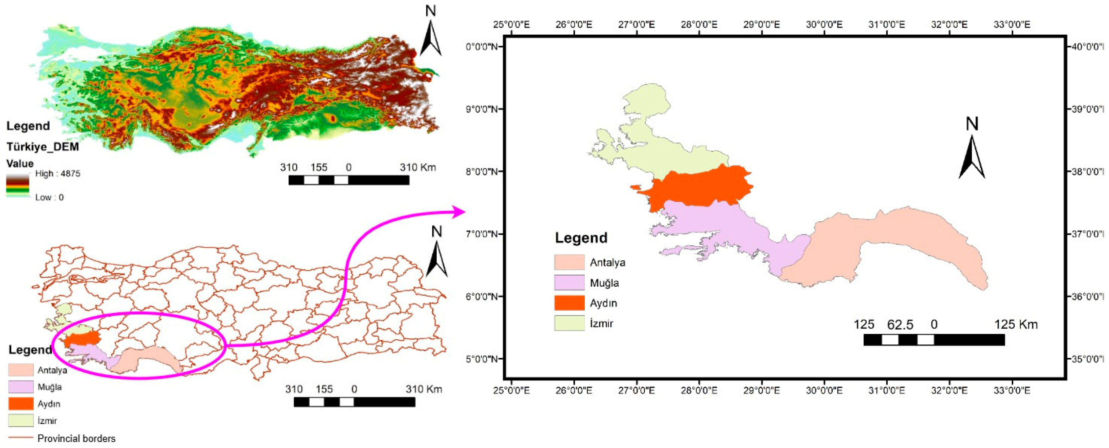
The study encompasses four coastal provinces in south-western Türkiye; namely, Antalya, Muğla, Aydın, and İzmir, as shown in Figure 1. These provinces collectively represent Türkiye’s most tourism-intensive coastal zone. Antalya and Muğla are internationally prominent mass-tourism destinations supported by major airport gateways, İzmir is the country’s third-largest metropolitan province [27] and a major Aegean maritime node, and Aydın combines coastal tourism with strong cruise-based and corridor-based seasonal mobility. To make the empirical basis of province selection more explicit, the basic demographic, tourism, and transport profile of the four provinces is summarized in

Table 1. Official demographic, tourism, and transport profile of the study provinces.

Province	Population	Accommodation Arrivals	Overnight Stays	Average Stay	Air Passengers	Cruise Passengers
Antalya	2,777,677	28,498,329	100,738,663	3.53	39,306,513	49,190
Muğla	1,099,547	5,541,130	18,327,167	3.31	10,038,127	235,447
Aydın	1,172,107	1,976,297	5,905,980	2.99	—	821,748
İzmir	4,504,185	3,373,417	6,889,113	2.04	11,512,096	230,094

. In this table, population values correspond to the latest official province-level resident population series for 2025 [27], whereas accommodation and transport indicators correspond to the latest complete annual tourism and mobility statistics available at the time of revision, namely the official 2024 accommodation, airport, and cruise statistics.

The values in Table 1 confirm that the selected provinces combine high tourism intensity with markedly different demographic and transport profiles. Antalya clearly dominates in accommodation arrivals and overnight stays, while Muğla also exhibits a strong tourism load relative to its population size. İzmir stands out by metropolitan scale and substantial air-passenger traffic, whereas Aydın is distinguished by exceptionally high cruise-passenger intensity through Kuşadası despite the absence of a directly comparable province-level commercial airport passenger total in the official year-end airport summaries. This diversity is methodologically important because it allows the proposed framework to be tested across provinces that belong to the same coastal tourism system but differ in urban scale, modal structure, and tourism-access configuration.

Recent official series further show that the study area is not static, but characterized by continuing demographic and tourism-related mobility change. While current population levels are reported in Table 1, recent tourism dynamics are more clearly seen in the official accommodation-arrival series [28]. Between 2023 and 2025, accommodation arrivals increased from 25.34 million to 28.50 million and then to 30.76 million in Antalya, from 5.15 million to 5.54 million and then to 9.13 million in Muğla, and from 3.29 million to 3.37 million and then to 4.20 million in İzmir. Aydın followed a slightly different pattern, declining marginally from 2.03 million in 2023 to 1.98 million in 2024, but then recovering to 2.51 million in 2025. These figures indicate that the tourism profile of the study area has remained strong overall, with continued growth in three provinces and only a temporary interruption in Aydın [28]. In transport terms, official gateway statistics show that airport passenger traffic increased between 2024 and 2025 in Antalya and İzmir and remained broadly stable at a very high level in Muğla [29], while maritime tourism continued to expand strongly in the Aegean part of the study area, particularly in Kuşadası and Bodrum. Since directly comparable annual modal-split series are not consistently reported at the provincial level across all four cases, the recent evolution of the transport context is represented here through official air and cruise passenger indicators, which constitute the most tourism-relevant interprovincial and international gateway flows in the study area. Taken together, these trends support the interpretation that Antalya, Muğla, Aydın, and İzmir represent not only the most tourism-intensive coastal zone of Türkiye in structural terms, but also an actively evolving tourism-transport setting in demographic and mobility terms [30].

3.2. Air Quality Station Data

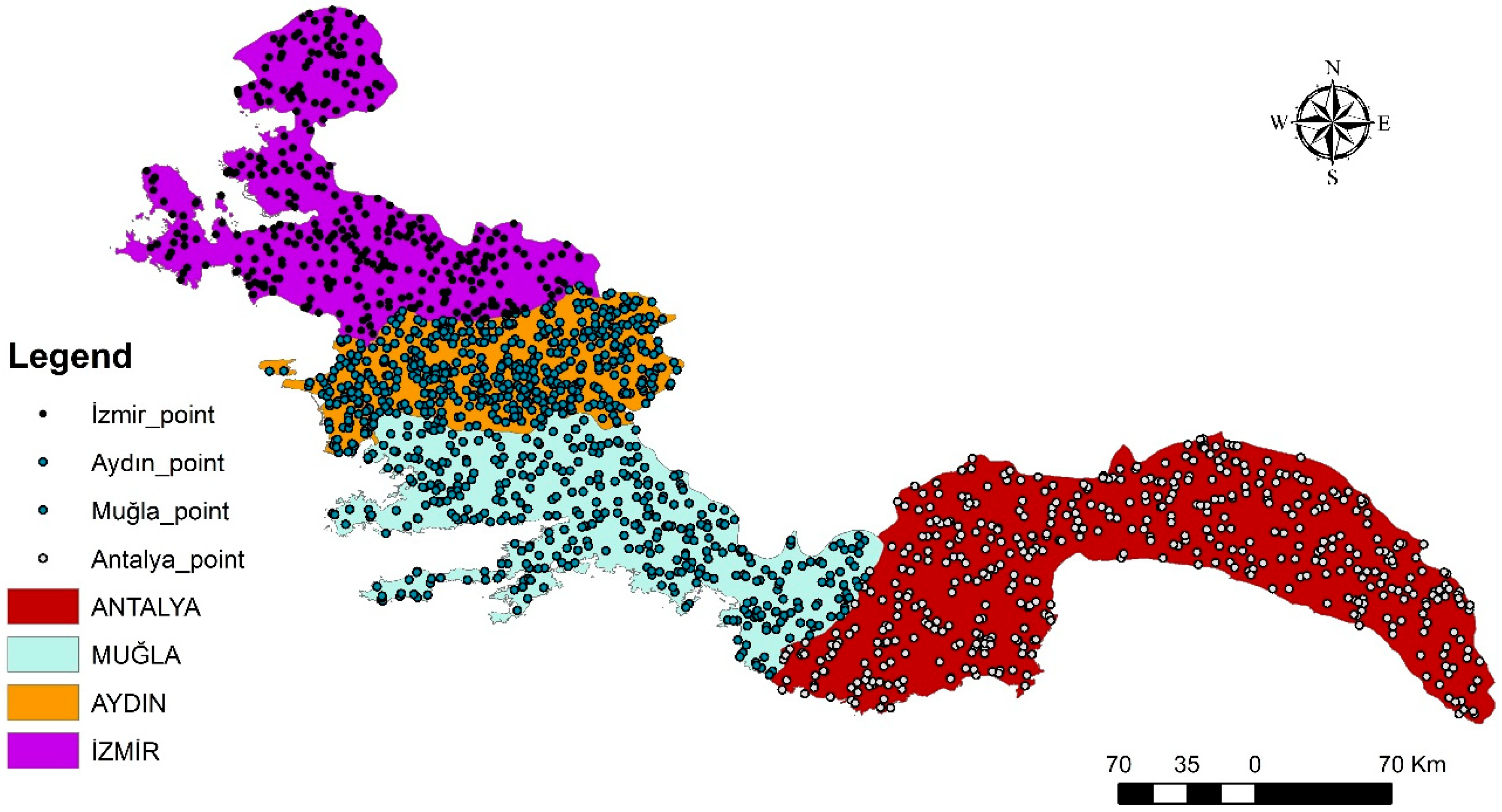
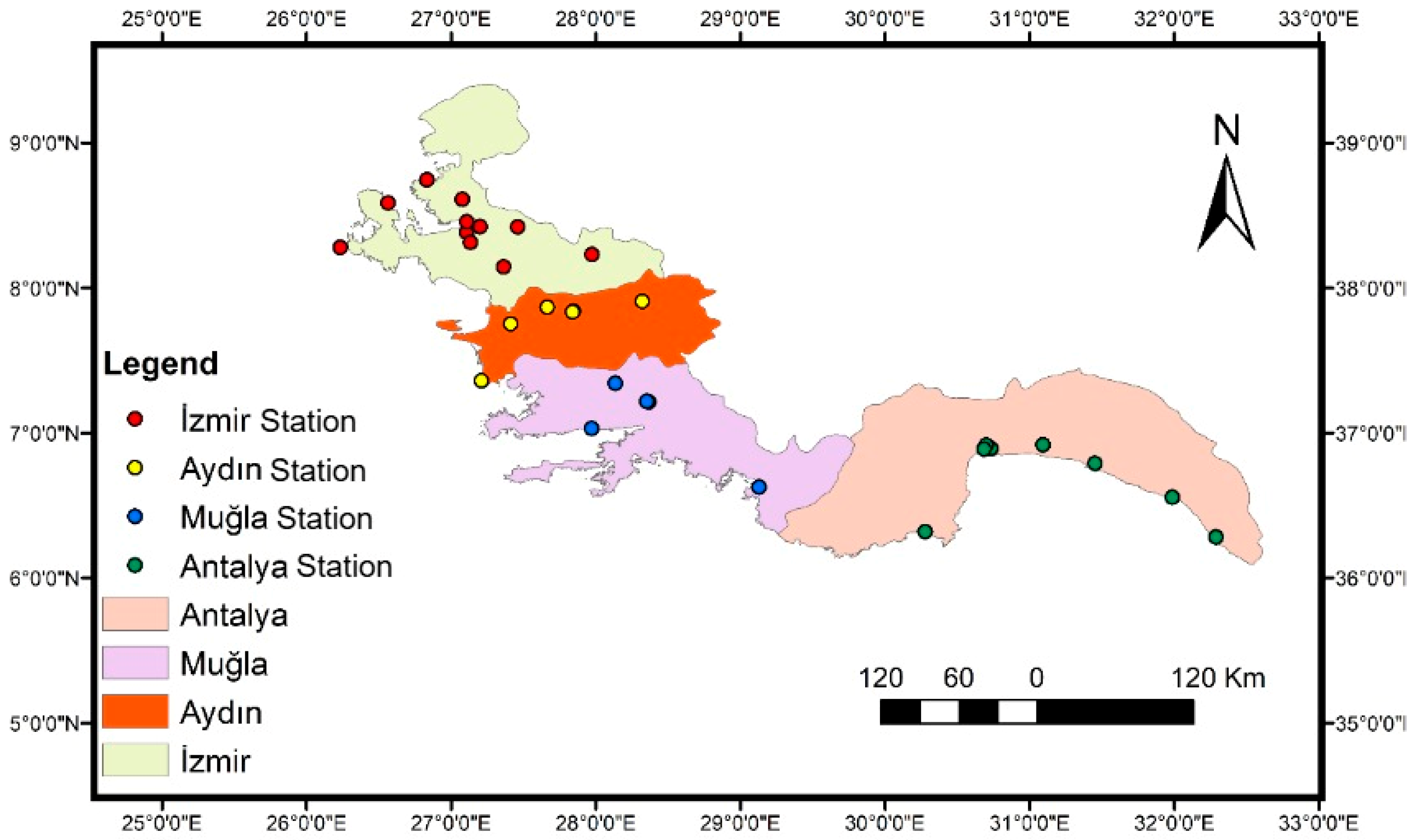
Air quality data were obtained from Türkiye’s National Air Quality Monitoring Network (UHKIA) for the retrospective one-year period from 25 January 2025 to 25 January 2026 [31]. The monitoring network used in this study comprised 35 stations distributed across the four study provinces; namely, 8 in Antalya, 6 in Muğla, 7 in Aydın, and 14 in İzmir. Their spatial distribution is shown in Figure 2. The pollutant set included PM10, SO₂, NO₂, NOx, NO, O₃, and CO. Seasonal representative values were derived using the median of daily observations for the summer (June–September) and winter (November–February) periods. Missing or invalid records in the downloaded station files were treated as NoData and were not converted to zero. To preserve the representativeness of the seasonal statistics, each station–pollutant–season combination was checked for data availability, and records with fewer than 10 valid measurement days within a season were excluded from the analysis. This threshold was set by the authors as a pragmatic minimum data-availability rule to avoid retaining highly sparse station–season combinations while preserving sufficient station coverage across provinces; however, no formal sensitivity analysis was conducted for this cutoff, and it should therefore be interpreted as a practical inclusion criterion. For NO and NOx, for which directly comparable short-term WHO guideline thresholds are not available, province- and season-specific P95 (N95) values calculated from pooled station-level seasonal medians were used as normalization references.

3.3. Spatial Criterion Layers for SUI

To construct the Spatial Suitability Index (SUI), a hierarchical framework consisting of 4 main criteria and 11 sub-criteria was established to represent the spatial structure of tourism- and transport-related pressure-context across the study area. Together, these criteria capture the main dimensions of coastal attractiveness, tourism and recreation intensity, accommodation structure, transport accessibility, population presence, and topographic conditions. This multi-criteria design was adopted to provide a spatially explicit and province-comparable representation of tourism-transport suitability beyond any single tourism or accessibility indicator. The complete criterion hierarchy, together with the thematic roles and spatial representations of all indicators, is presented in

Table 2. Main and sub-criteria used in the construction of the SUI map.

Main Criterion	Sub-Criterion	Spatial Layer	Aspect
C1: Coastal Attractiveness and Recreation	C1.1 Coastal proximity	Distance-decay from shoreline	Benefit
	C1.2 POI density	Kernel density of tourist POIs	Benefit
C2: Accommodation and Tourism Demand	C2.1 Accommodation supply density	Bed capacity per unit area	Benefit
	C2.2 Tourist arrivals	District-level annual arrivals	Benefit
	C2.3 Avg. length of stay	District-level mean overnight duration	Benefit
	C2.4 Hotel count	Licensed accommodation units	Benefit
C3: Transport Accessibility and Mobility	C3.1 Road network density	Road length per unit area	Benefit
	C3.2 Junction/node density	Intersection count per unit area	Benefit
	C3.3 Transfer node accessibility	Distance-decay from airports/terminals	Benefit
C4: Exposure and Topographic Modulation	C4.1 Population density	Population per unit area	Benefit
	C4.2 Topographic elevation	SRTM DEM	Cost

.

Taken together, the four criterion groups operationalize a pressure-context logic rather than a direct flow or emission inventory. More specifically, C1 represents attraction intensity, C2 captures accommodation structure and tourism-demand concentration, C3 reflects accessibility and movement potential, and C4 describes exposure-context modulation through population presence and topographic conditions. The analytical assumption is that areas where these dimensions co-concentrate are more likely to host intensified tourism-related activity and associated mobility demand. The SUI was therefore designed to identify where tourism-transport pressure is more likely to accumulate spatially, not to measure realized traffic, tourist flows, or emissions directly.

The present framework does not incorporate direct dynamic activity indicators such as traffic counts, real-time tourist flows, or emission inventories. Instead, the tourism-transport context is operationalized through a province-comparable set of spatial proxy variables that jointly represent tourism demand, accommodation intensity, attraction structure, and accessibility conditions. In this respect, tourist arrivals, average length of stay, hotel count, accommodation supply density, coastal attractiveness, and POI density were used to reflect the tourism dimension, while road network density, junction/node density, and transfer node accessibility were used to represent the transport and mobility context. This proxy-based structure was preferred because it enabled the construction of a consistent GIS framework across all four provinces using spatially available and comparable datasets. Emission variables were not incorporated into the SUI itself, since air pollution was already analyzed separately through observed monitoring-based pollutant surfaces; including emission-related variables within the SUI would have reduced the conceptual distinction between the explanatory pressure-context layer and the environmental outcome layer. Accordingly, the results should be interpreted as evidence of empirical spatial association between tourism-transport context and seasonal pollution burden, rather than as proof of a direct flow-based or emission-based causal mechanism.

3.4. Expert Decision-Making Team

Because the construction of the SUI map involves a multi-criteria structure composed of four main criteria and eleven sub-criteria, the weighting stage required expert-based evaluation to determine the relative importance of the indicators in a spatially meaningful and methodologically consistent way. In multi-criteria decision-making studies, the composition of the expert team is a critical step, particularly when the problem involves the simultaneous consideration of infrastructure, accessibility, land-use structure, and tourism-related spatial dynamics [32]. Previous studies have often shown that a relatively small but competent expert group, commonly within the range of 3 to 7 participants, can be adequate for structured weighting procedures, provided that the participants are able to apply the comparison logic consistently and interpret the decision problem in a coherent way [32,33,34]. In this study, a four-member decision-making team was therefore considered appropriate as a workable balance between disciplinary input, consistency of judgment, and the practical requirements of the applied MCDM framework.

The expert panel consisted of three civil engineering academics and one urban planner. Although the panel did not include specialists from air quality, atmospheric science, tourism economics, or environmental health, the selected experts were not limited to a narrow transport-engineering perspective. The civil engineering academics had relevant experience in sustainable transport, infrastructure systems, GIS-based spatial analysis, and environmentally sensitive transport evaluation, while the urban planner contributed a planning-oriented perspective on tourism space, settlement structure, and land-use organization. In addition, for methods such as AHP and Fuzzy SIWEC, domain knowledge alone is not sufficient; the structured application of pairwise or linguistic weighting procedures also requires methodological familiarity and the ability to produce interpretable and internally coherent judgments. For this reason, the panel was selected not only on the basis of topical relevance, but also with regard to its capacity to apply the MCDM procedure in a stable and usable form.

The role of the expert team extended beyond the assignment of numerical weights. Before the weighting stage, the proposed criterion hierarchy was presented to the experts in a structured format, and they were asked to review whether the selected criteria were relevant and sufficiently representative for capturing the spatial dimensions of tourism-transport pressure-context across the four provinces. This review informed the final organization of the criteria prior to weighting. However, this step should not be interpreted as a formal validation exercise in the Delphi sense. No multi-round Delphi procedure, formal consensus protocol, or separate questionnaire-based validation process was conducted. Instead, the study adopted a single-round expert review and weighting design within the scope of a methodology-intensive framework. This choice allowed the study to keep the analytical procedure manageable within a single article, but it also constitutes a limitation. In particular, the absence of a broader disciplinary panel and a formal consensus-based validation stage means that the criterion structure should be understood as expert-informed and methodologically screened rather than externally validated through a separate consensus process.

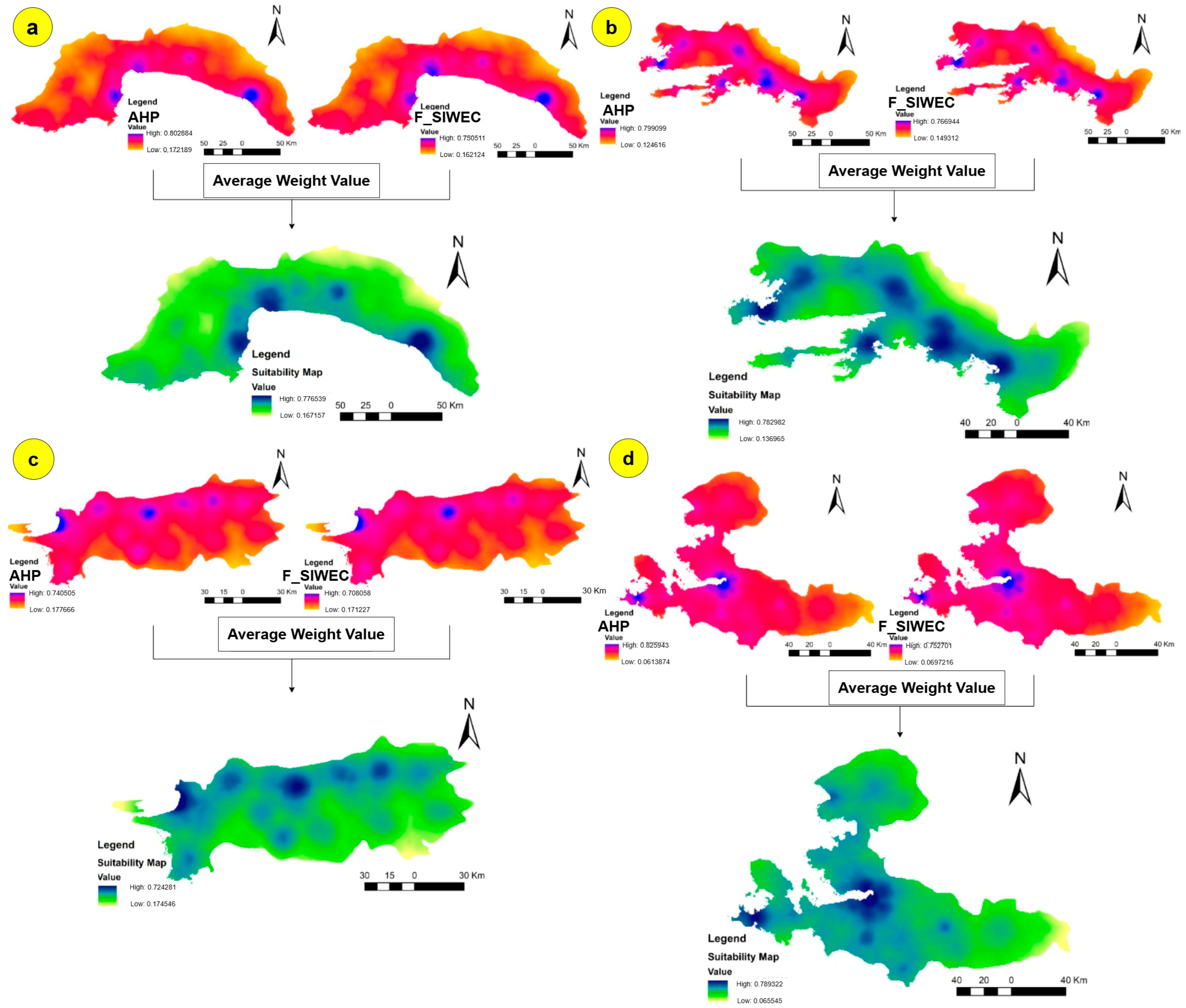
The authors acknowledge that expert-based weighting inherently involves a degree of subjectivity, particularly in a multi-criteria framework where the final SUI depends on the relative importance assigned to the sub-criteria. For this reason, the study did not rely on a single weighting method. Instead, two conceptually different approaches—namely, AHP and Fuzzy SIWEC—were implemented in parallel, and their outputs were reported separately before constructing the integrated SUI. The close spatial correspondence observed between the two method-specific suitability surfaces suggests that the dominant spatial pattern is broadly stable across alternative weighting schemes, even though local intensity differences remain visible. In addition, the detailed AHP calculations, including expert-specific pairwise comparison matrices and consistency statistics, are provided in File S1 to improve transparency. Nevertheless, the authors recognize that a more extensive formal sensitivity analysis of expert-derived weights would further strengthen the framework and should be considered in future research.

4. Methodology

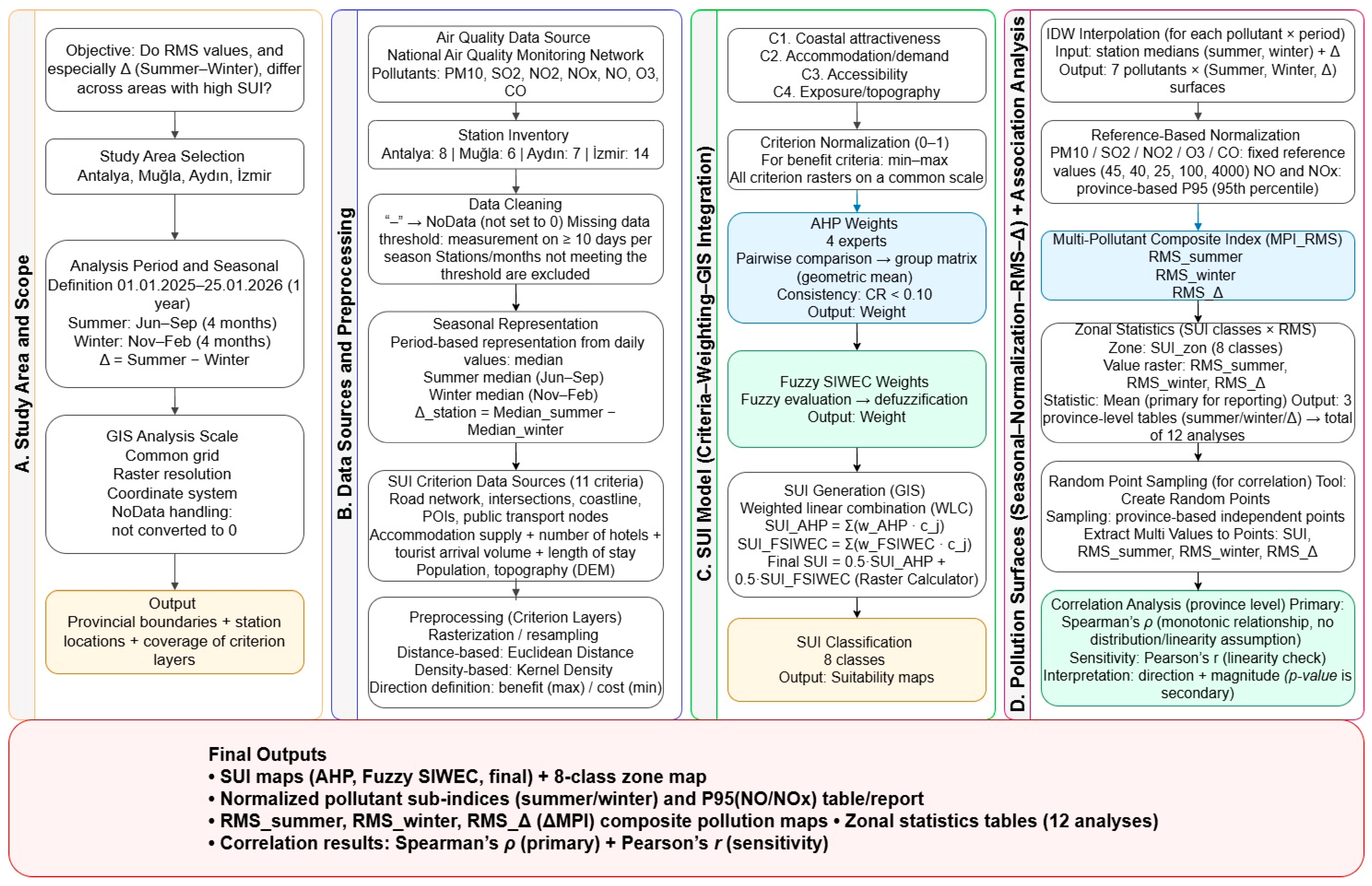
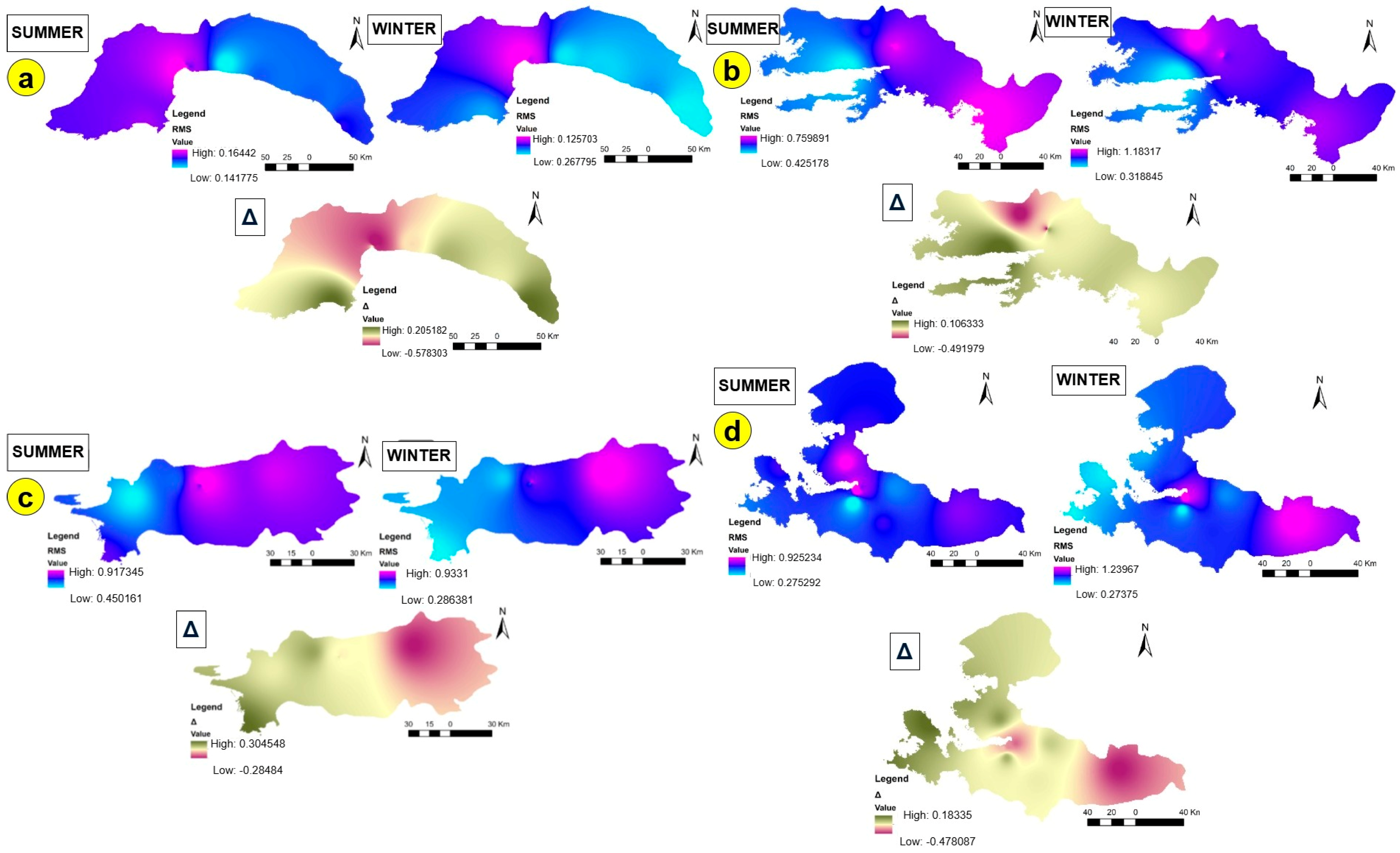
The methodological framework of this study was designed to examine whether tourism- and transport-related spatial suitability is associated with seasonal multi-pollutant air quality patterns across the selected coastal provinces. As summarized in Figure 3, the workflow consists of four interrelated stages. First, the study area, temporal scope, and common GIS analysis framework were defined to ensure spatial and seasonal comparability across Antalya, Muğla, Aydın, and İzmir. Second, air quality data obtained from the National Air Quality Monitoring Network were cleaned, seasonally aggregated, and prepared for spatial interpolation, while the 11 SUI criteria layers were compiled and standardized within a common raster environment. Third, the SUI model was constructed by weighting the criteria through AHP and Fuzzy SIWEC and integrating them in a GIS-based weighted overlay procedure. Finally, seasonal pollutant surfaces were generated, normalized using pollutant-specific reference thresholds and province-based P95 values for NO and NOx, and then combined into composite RMS-based pollution indicators for summer, winter, and seasonal difference conditions. These outputs were subsequently linked to the SUI surface through zonal statistics and province-level correlation analyses in order to evaluate the magnitude and direction of the relationship between tourism-transport pressure-context and seasonal pollution burden. In this way, the framework integrates spatial suitability modeling, seasonal pollution mapping, and statistical association analysis within a unified methodological structure.

4.1. Tourism-Transport Suitability Index (SUI)

In this study, the Tourism-Transport Suitability Index (SUI) should not be interpreted as a direct measure of realized tourism-transport flows, emissions, or observed traffic intensity. Rather, it represents a spatially explicit pressure-context surface that captures the relative likelihood of tourism- and transport-related activity concentrating in particular locations. This conceptualization was adopted because the analysis required a common and province-comparable indicator framework that could be constructed consistently for all four study areas using spatially available datasets. Accordingly, the SUI was derived from 11 criteria reflecting coastal attractiveness, recreation intensity, accommodation structure, accessibility, population presence, and topographic conditions, all of which function as enabling or amplifying factors of tourism-transport concentration. In this sense, the index represents potential spatial pressure rather than directly observed pressure, and it is used as a common analytical reference surface for examining whether areas characterized by stronger tourism-transport context also display systematically different seasonal multi-pollutant patterns. To derive criterion weights in a robust and methodologically transparent manner, two complementary multi-criteria decision-making approaches were employed: the Analytic Hierarchy Process (AHP) and fuzzy SIWEC. The use of both methods served two purposes. First, AHP provided a well-established hierarchical comparison framework with an explicit consistency check. Second, fuzzy SIWEC enabled the incorporation of uncertainty embedded in expert judgments by allowing decision-makers to express their assessments through linguistic terms rather than exact numerical values. The resulting weights obtained from both methods were subsequently transferred to the GIS environment and integrated into the raster-based weighted overlay procedure to generate the final spatial suitability surface.

4.1.1. Analytic Hierarchy Process (AHP)

The Analytic Hierarchy Process, originally developed by Saaty, is one of the most widely used multi-criteria decision-making methods for structuring complex decision problems and deriving relative criterion weights from pairwise comparisons [35]. Its analytical strength lies in combining hierarchical problem decomposition, reciprocal pairwise judgments, eigenvector-based prioritization, and formal consistency testing within a single framework. In the present study, AHP was used to quantify the relative importance of the evaluation criteria through expert-based judgments.

The AHP procedure consisted of three sequential stages. First, the decision problem was structured hierarchically by defining the overall objective at the top level, the main and sub-criteria at the intermediate level, and the alternatives or spatial outputs at the lowest level. Second, pairwise comparison matrices were constructed using Saaty’s 1–9 importance scale, where 1 indicates equal importance and 9 indicates extreme importance; intermediate even numbers were used when compromise values were needed. The reciprocal rule was applied such that, if criterion was assigned a preference value of x over criterion j, then the inverse comparison was represented as 1/x.

Let $A=\left[a_{ij}\right]$ denote the pairwise comparison matrix, where $a_{ij}$ represents the relative importance of criterion over criterion j, subject to the reciprocal condition $a_{ij}$ = 1/$a_{ji}$. After the comparison matrix was formed, the priority vector representing the relative criterion weights was derived. Following a widely used computational approach, the matrix was normalized column-wise and the arithmetic mean of each row in the normalized matrix was calculated to obtain the weight vector. Accordingly, the resulting priority vector is given in Equation (1).

$$w_i={\displaystyle \frac{1}{n}}{\displaystyle {\sum }_{j=1}^n}{a}_{ij,}i=1,2,\dots ,n$$

(1)

where ${\overline{a}}_{ij}$ denotes the normalized entry of the comparison matrix and n is the number of criteria. The resulting weights satisfy the condition ${\sum }_{i=1}^n{w}_i=1$.

When multiple experts are involved, individual judgments can be aggregated into a single comparison matrix using the geometric mean, which preserves the reciprocal structure of the AHP matrix. Thus, if m experts evaluate the same criterion pair, the aggregated comparison value is given in Equation (2).

$$a_{ij}^{\mathrm{*}}={\left({\displaystyle {\prod }_{k=1}^m}{a}_{ij}^{\left(k\right)}\right)}^{1/m}$$

(2)

where $a_{ij}^{\left(k\right)}$ is the comparison assigned by expert k.

A critical stage of AHP is the evaluation of judgment consistency. For this purpose, the Consistency Index (CI) and the Consistency Ratio (CR) were computed. The CI was calculated using Equation (3).

$$CI={\displaystyle \frac{{\lambda }_{max}-n}{n-1}}$$

(3)

where ${\lambda }_{max}$ is the maximum eigenvalue of the comparison matrix and n is the matrix order. The CR was then obtained by dividing the consistency index by the Random Index (RI), as shown in Equation (4).

$$CR={\displaystyle \frac{CI}{RI}}$$

(4)

According to the widely accepted decision rule in the AHP literature, a matrix is considered acceptably consistent when CR ≤ 0.10. If the calculated CR exceeds 0.10, the pairwise judgments should be reviewed and revised before the derived weights are interpreted. In the present study, only consistency-approved weight sets were retained for subsequent GIS-based suitability modeling.

4.1.2. Fuzzy SIWEC

In addition to AHP, fuzzy SIWEC was employed to determine criterion weights while explicitly incorporating uncertainty in expert judgments. The SIWEC method, originally introduced as a simple weight calculation approach, offers a comparatively parsimonious alternative to pairwise comparison-based methods because it allows decision-makers to evaluate criteria directly rather than comparing all criteria against one another. Its fuzzy extension further improves the method by enabling the use of linguistic assessments and triangular fuzzy numbers, which are more compatible with the ambiguity and imprecision inherent in expert-based reasoning [36].

The rationale for using fuzzy SIWEC in this study is methodological as well as practical. As the number of criteria increases, methods based on full pairwise comparison structures may become cognitively demanding and more prone to inconsistency. By contrast, fuzzy SIWEC permits experts to assign importance levels directly through linguistic terms such as low, medium, and high, thereby reducing assessment burden while preserving uncertainty information. The linguistic terms and their corresponding triangular fuzzy numbers are presented in

Table 3. Matching linguistic terms with membership functions.

Linguistic Terms	Abbreviation	Membership Function
Absolutely bad	AB	(1,1,1)
Very bad	VB	(1,2,3)
Bad	B	(2,3,4)
Medium-bad	MB	(3,4,5)
Equal	E	(4,5,6)
Medium-good	MG	(5,6,7)
Good	G	(6,7,8)
Extremely good	EG	(7,8,9)
Absolutely good	AG	(8,9,10)
Perfect	P	(9,10,10)

.

In the fuzzy SIWEC procedure, each expert evaluated the importance of criterion j using a linguistic expression represented by a triangular fuzzy number. Accordingly, the fuzzy evaluation of criterion j by expert i is given in Equation (5).

$${\tilde{x}}_{ij}=\left(x_{ij,}^l{x}_{ij,}^m{x}_{ij,}^u\right)$$

(5)

where $x_{ij, }^l{x}_{ij, }^m \mathrm{a}\mathrm{n}\mathrm{d} x_{ij}^u$ denote the lower, modal, and upper bounds of the triangular fuzzy number, respectively. After fuzzification, the individual judgments were assembled into the fuzzy decision matrix given in Equation (6).

$$\tilde{A}=\left[\begin{array}{c}{\check{x}}_{11}\\ {\check{x}}_{21}\\ \begin{array}{c}\dots \\ ⋮\\ \begin{array}{c}\dots \\ {\check{x}}_{m1}\end{array}\end{array}\end{array}\begin{array}{c}{\check{x}}_{12}\\ {\check{x}}_{22}\\ \begin{array}{c}\dots \\ ⋮\\ \begin{array}{c}\dots \\ {\check{x}}_{m2}\end{array}\end{array}\end{array}\begin{array}{c}\dots \\ \dots \\ \begin{array}{c}\dots \\ ⋮\\ \begin{array}{c}\dots \\ \dots \end{array}\end{array}\end{array}\begin{array}{c}{\check{x}}_{1n}\\ {\check{x}}_{2n}\\ \begin{array}{c}\dots \\ ⋮\\ \begin{array}{c}\dots \\ {\check{x}}_{mn}\end{array}\end{array}\end{array}\right]$$

(6)

where m is the number of experts and n is the number of criteria.

To make the fuzzy values comparable across criteria and experts, the decision matrix was normalized. In this study, normalization was performed by dividing each triangular fuzzy number by the maximum upper bound observed within the relevant set of evaluations. Thus, the normalized fuzzy value was computed using Equation (7).

$${\tilde{n}}_{ij}={\displaystyle \frac{x_{ij}^l}{\max x_{ij}^u}},{\displaystyle \frac{x_{ij}^m}{\max x_{ij}^u}},{\displaystyle \frac{x_{ij}^u}{\max x_{ij}^u}}$$

(7)

This step ensured homogeneity across the fuzzy assessments and improved the interpretability of the subsequent aggregation process. Following normalization, the variability of the expert evaluations was incorporated through the standard deviation. This step was intended to account for the degree of dispersion in the normalized judgments and to reduce the influence of inconsistent assessments. The adjusted fuzzy value was obtained by multiplying the normalized value by the corresponding standard deviation, as shown in Equation (8).

$${\tilde{v}}_{ij}={\tilde{n}}_{ij} x {\sigma }_j$$

(8)

where ${\sigma }_j$ denotes the standard deviation associated with criterion j. This adjustment step follows the original fuzzy SIWEC formulation proposed by [36]. In that method, the standard deviation is not used merely as a descriptive uncertainty statistic, but as an adjustment factor that gives greater importance to decision-makers whose evaluations are more differentiated. Accordingly, the multiplication in Equation (8) was retained here as part of the original published procedure rather than introduced as a new aggregation choice in the present study.

The expert opinions were then aggregated criterion-wise to obtain cumulative fuzzy scores, as shown in Equation (9).

$${\tilde{s}}_{ij}={\sum }_{j=1}^m{\tilde{v}}_{ij}$$

(9)

Based on these cumulative fuzzy values, the relative fuzzy weights were calculated using Equation (10).

$${\tilde{w}}_{ij}={\displaystyle \frac{s_{ij}^l}{{\sum }_{j=1}^n{s}_{ij}^u}},{\displaystyle \frac{s_{ij}^m}{{\sum }_{j=1}^n{s}_{ij}^m}},{\displaystyle \frac{s_{ij}^u}{{\sum }_{j=1}^n{s}_{ij}^l}}$$

(10)

where $s_{ij}^l$, $s_{ij}^m$, and $s_{ij}^u$ denote the lower, modal, and upper components of the aggregated fuzzy score for criterion j.

In the final stage, the fuzzy weights were converted into crisp values using the defuzzification formula given in Equation (11), as adopted in the original fuzzy SIWEC framework.

$$w_{jdef}={\displaystyle \frac{w_{ij}^l+4.w_{ij}^m+w_{ij}^u}{6}}$$

(11)

where $w_{ij}^l$, $w_{ij}^m$, and $w_{ij}^u$ are the lower, modal, and upper components of the fuzzy weight. The resulting crisp values represent the final criterion weights derived from fuzzy SIWEC. For consistency in GIS implementation, the defuzzified values were subsequently normalized so that the total weight sum equalled 1.

4.1.3. GIS-Based Weighted Linear Combination

GIS-based weighted linear combination constitutes one of the most widely adopted integration procedures in spatial decision-making studies, particularly in applications where multiple heterogeneous criteria must be synthesized into a single tourism-transport pressure-context surface. Its broad applicability has been demonstrated across a wide range of planning and site-selection problems, including electric vehicle charging station (EVCS) siting [37,38], micro mobility planning [39,40], landfill and waste facility location [41,42], the logistic center [43], green hydrogen plant [44], and solar power plant [45]. In such contexts, the method enables the simultaneous consideration of diverse spatial variables within a transparent and reproducible analytical framework.

In the present study, the criterion weights derived from AHP and fuzzy SIWEC were transferred to the GIS environment for raster-based spatial integration. A separate raster layer was prepared for each criterion in ArcMap 10.6, and each raster was multiplied by its corresponding weight coefficient. Since all criterion layers had previously been standardized to a common scale, the weighted linear combination procedure made it possible to integrate them into a single composite suitability surface while preserving the relative influence assigned to each criterion during the weighting stage.

The final suitability surface was generated using the weighted overlay formulation given in Equation (12).

$$S={\displaystyle {\sum }_{j=1}^n}{w}_j.r_j$$

(12)

where S denotes the final suitability score, $w_j$ is the weight assigned to criterion j, and $r_j$ is the normalized raster value of criterion j. This formulation ensures that the final score at each raster cell reflects the cumulative contribution of all criteria according to their relative importance.

The procedure was applied separately for the AHP and fuzzy SIWEC derived weight sets, thereby producing two method-specific suitability surfaces. In the final stage, these outputs may either be interpreted individually for comparative purposes or integrated into a consensus suitability map, depending on the analytical strategy adopted in the manuscript. This approach allows the study not only to generate the final SUI surface, but also to evaluate the degree to which alternative weighting schemes influence the resulting spatial pattern.

4.2. Multi-Pollutant Air Pollution Surfaces

4.2.1. IDW Spatial Interpolation

To characterize the spatial and seasonal variability of air pollution across the study area, station-based observations were first reduced to seasonal representative values and then transformed into continuous raster surfaces. Seasonal representation was based on the median of daily observations for each pollutant and each station, separately for summer (June–September) and winter (November–February). The median was preferred because it provides a more robust summary of seasonal central tendency under short-term peaks, episodic outliers, and irregular measurement continuity. Records with insufficient seasonal coverage were excluded from further analysis, and missing observations were retained as NoData rather than converted to zero in order to avoid artificial underestimation of pollution levels.

The study covered a total of 35 monitoring stations distributed across Antalya, Muğla, Aydın, and İzmir, and the pollutant set comprised PM10, SO₂, NO₂, NOx, NO, O₃, and CO. Using these seasonal median station values, spatial concentration surfaces were generated for each pollutant by means of Inverse Distance Weighting (IDW) interpolation. In the interpolation stage, IDW was implemented using the conventional power parameter of p = 2. This setting was adopted as a practical default for comparative provincial surface generation within the ArcMap environment. This procedure produced, for each province and pollutant, at least two primary seasonal surfaces representing summer and winter conditions; in addition, a seasonal contrast layer was subsequently derived to represent inter-seasonal change.

Because the number of province–pollutant–season outputs was high, all individual IDW surfaces were not presented visually in the main text. Nevertheless, the full set of pollutant surfaces was generated prior to the normalization and multi-pollutant aggregation stages. The interpolated pollutant rasters were then harmonized within the common spatial framework adopted throughout the analysis. Since all raster outputs were transferred to a shared grid structure with the same cell size, projection, and analysis extent, the air pollution surfaces were treated as spatially comparable inputs for the subsequent normalization and composite-index procedures.

IDW was adopted as a practical interpolation approach suitable for comparative provincial analysis. However, because it is not physically constrained by topography or atmospheric dynamics, the resulting surfaces should be interpreted as comparative spatial approximations rather than exact atmospheric fields. In areas with sparse monitoring coverage or more complex source structures, some degree of interpolation uncertainty is therefore unavoidable. For this reason, future studies may benefit from comparing IDW with alternative interpolation techniques and uncertainty assessment procedures.

An additional scale-related consideration should also be noted. Because the interpolation procedure transforms station-based observations into continuous provincial surfaces, and because the subsequent analysis relies on composite and class-based representations, localized hotspots may become spatially smoothed during the analytical process. This does not invalidate the comparative value of the resulting surfaces, but it does mean that highly localized pollution signals associated with specific corridors, nodes, or destination clusters may be attenuated when interpreted at the provincial scale. Accordingly, the interpolated and aggregated outputs should be read as comparative regional patterns rather than as fully hotspot-preserving representations of local emission intensity.

No formal cross-validation or error-based interpolation assessment (RMSE or MAE) was conducted for the full set of pollutant–province–season outputs. Given the comparative scope of the study and the large number of generated surfaces, the interpolation step was used as a practical spatial approximation procedure rather than as a separately optimized geostatistical modeling exercise. This limitation is particularly relevant in provinces with sparser monitoring coverage and more complex geography, such as Muğla, where interpolation uncertainty may be higher. Accordingly, the resulting surfaces should be interpreted as comparative regional patterns derived from the available monitoring framework, not as fully validated hotspot-accurate atmospheric fields.

4.2.2. Reference Normalization and RMS Aggregation

Because the selected pollutants differ substantially in numerical magnitude and exposure scale, their raw concentration surfaces could not be meaningfully combined without prior standardization. A reference-based normalization approach was therefore adopted, in which each interpolated pollutant surface was divided by a pollutant-specific reference value in order to produce a dimensionless sub-index. This transformation was essential for preventing pollutants with numerically larger concentration ranges, such as CO, from dominating the combined metric solely because of scale differences. Under this framework, the normalized pollutant sub-index for pollutant p in season s is defined as shown in Equation (13):

$$I_{p,s}={\displaystyle \frac{C_{p,s}}{{Ref}_p}}$$

(13)

where $C_{p,s}$ denotes the IDW-derived concentration raster for pollutant p in season s, and ${Ref}_p$ is the selected reference threshold. The resulting $I_{p,s}$ surfaces are dimensionless and directly interpretable: values close to 1 indicate concentrations around the reference level, values greater than 1 indicate local exceedance, and values below 1 indicate sub-threshold conditions.

For PM10, SO₂, NO₂, O₃, and CO, short-term [46] values were used as fixed health-based reference thresholds: 45 µg/m³ for PM10 (24 h), 40 µg/m³ for SO₂ (24 h), 25 µg/m³ for NO₂ (24 h), 100 µg/m³ for O₃ (daily maximum 8 h), and 4 mg/m³ for CO, converted to 4000 µg/m³ for unit consistency.

For NO and NOx, a different scaling strategy was required because directly comparable short-term WHO thresholds were not available for the temporal structure used in the analysis. To avoid instability arising from maxima or highly episodic values, a province and season-specific P95/N95 reference framework was adopted. In this procedure, station-based seasonal medians for NO and NOx were first calculated for each province and season, then pooled within each province, and finally the 95th percentile of those medians was used as the normalization reference. This approach served two purposes: it constrained the influence of episodic spikes and, at the same time, represented the upper range of typical high concentrations in a more stable and interpretable way. The mixed normalization strategy therefore reflects the unequal availability of directly comparable short-term reference thresholds across the selected pollutants. While WHO-based thresholds provided externally defined health-oriented reference points for PM10, SO₂, NO₂, O₃, and CO, P95-based scaling was used for NO and NOx in order to retain these transport-sensitive pollutants within the composite structure. Accordingly, the normalized sub-indices should not be interpreted as carrying identical toxicological meaning across all pollutants; rather, they provide a common dimensionless basis for comparative spatial interpretation within the analytical framework of the study. For this reason, the resulting RMS surface should be interpreted as a reference-normalized relative multi-pollutant burden indicator, not as a universal risk-equivalent metric with full cross-pollutant or cross-provincial toxicological equivalence.

Following normalization, the seven pollutant-specific sub-indices were aggregated into a multi-pollutant composite surface using the Root Mean Square (RMS) approach given in Equation (14).

$${RMS}_s=\sqrt{{\displaystyle \frac{1}{n}}{\displaystyle {\sum }_{p=1}^n}{I}_{p,s}^2}$$

(14)

where n denotes the number of pollutants. RMS was preferred over simpler alternatives for three main reasons. First, tourism-transport effects are not expected to emerge through a single pollutant alone, but rather through simultaneous changes in multiple pollutants; RMS therefore summarizes the multi-signal structure within one interpretable surface. Second, because the method squares the normalized sub-indices prior to aggregation, pollutants with relatively high sub-index values exert a stronger influence than they would under simple arithmetic averaging; this reduces the risk that local peaks disappear in the combined surface. Third, because all inputs are normalized relative to reference values, the RMS framework combines pollutants on a common dimensionless basis and ensures that the final composite reflects relative burden rather than raw numerical magnitude. In this sense, the RMS surface should be interpreted as a reference-normalized relative multi-pollutant burden indicator rather than as a direct measure of cumulative exposure risk or epidemiological health impact. Its role in the present study is comparative and interpretive; namely, to identify where compound seasonal burden becomes more visible within the common spatial framework.

To evaluate interseasonal change, a signed summer-winter difference layer was defined using Equation (15).

$$∆MPI={RMS}_{summer}-{RMS}_{winter}$$

(15)

where positive values indicate that the composite burden is higher in summer and negative values indicate winter dominance. In addition, an unsigned seasonal fluctuation metric may be reported, if required, to capture the magnitude of seasonal change irrespective of direction. Within the present analytical design, however, the signed summer-winter contrast constitutes the more informative layer because it allows interseasonal variation to be interpreted in relation to tourism-season intensity. Importantly, this contrast layer should be understood as a tool for examining whether tourism-season-related changes become spatially visible, rather than as a direct measure of causal or directly attributable health increment.

The interpolated pollution surfaces constitute the direct basis of the subsequent RMS aggregation, zonal statistics, and correlation analyses. For this reason, interpolation uncertainty should be regarded as a central methodological constraint rather than as a peripheral limitation, particularly in provinces where monitoring-station density is lower and spatial coverage is more uneven. The resulting surfaces should therefore be interpreted as comparative spatial approximations derived from the available monitoring framework, not as exact atmospheric fields. In addition, the RMS-based composite index should not be interpreted as a direct measure of cumulative exposure risk or epidemiological health impact. Rather, it represents a reference-normalized relative multi-pollutant burden indicator that summarizes the simultaneous spatial prominence of multiple pollutants on a common dimensionless scale. Because the RMS formulation gives greater influence to relatively high normalized sub-index values, it is analytically useful for identifying areas where compound seasonal burden becomes more visible; however, its function in the present study is comparative and interpretive, not clinical or dose–response based.

4.3. SUI–Pollution Linkage Analysis

To evaluate the spatial relationship between the Spatial Suitability Index (SUI) and the multi-pollutant air pollution indicators, a two-stage linkage strategy based on zonal statistics and point-based correlation analysis was employed.

The methodological framework of this study should be interpreted as a spatial association design rather than a direct causal pressure model. Specifically, the analysis constructs two analytically distinct but spatially comparable surfaces: a Tourism-Transport Suitability Index (SUI) derived from expert-weighted spatial criteria, and seasonal multi-pollutant burden surfaces derived from interpolated monitoring data. The purpose of the framework is not to assume that one surface mechanically determines the other, but to examine whether areas characterized by stronger tourism-transport context display systematically different seasonal pollution patterns within the same provincial spatial setting. In this sense, the study evaluates an empirical spatial relationship and seasonal co-occurrence structure, rather than a direct flow-based or emission-based causal linkage. This distinction clarifies that the SUI represents a pressure-context surface based on enabling and amplifying spatial factors, whereas the pollution maps represent observed environmental conditions derived from monitoring data.

In the first stage, the final SUI raster was classified into eight classes using the Natural Breaks (Jenks) method in ArcMap in order to create an interpretable zoning structure for the subsequent class-based analysis. This method was preferred because it identifies breakpoints from the internal empirical distribution of SUI values, and was therefore considered more suitable than equal-interval or quantile-based classification for representing the major gradients of the suitability surface in the present dataset. The summer, winter, and seasonal-difference RMS surfaces were then summarized within these SUI classes using the ArcMap Zonal Statistics tool. For article-level consistency and methodological robustness, class-based median values were used, as they align with the median-based seasonal representation of station observations and reduce the influence of raster-level extremes. The purpose of this step was to assess whether composite pollution burden varies systematically across ordered SUI levels, whether seasonal contrasts become more visible in specific suitability classes, and whether areas characterized by similar suitability levels display different seasonal pollution patterns across provinces.

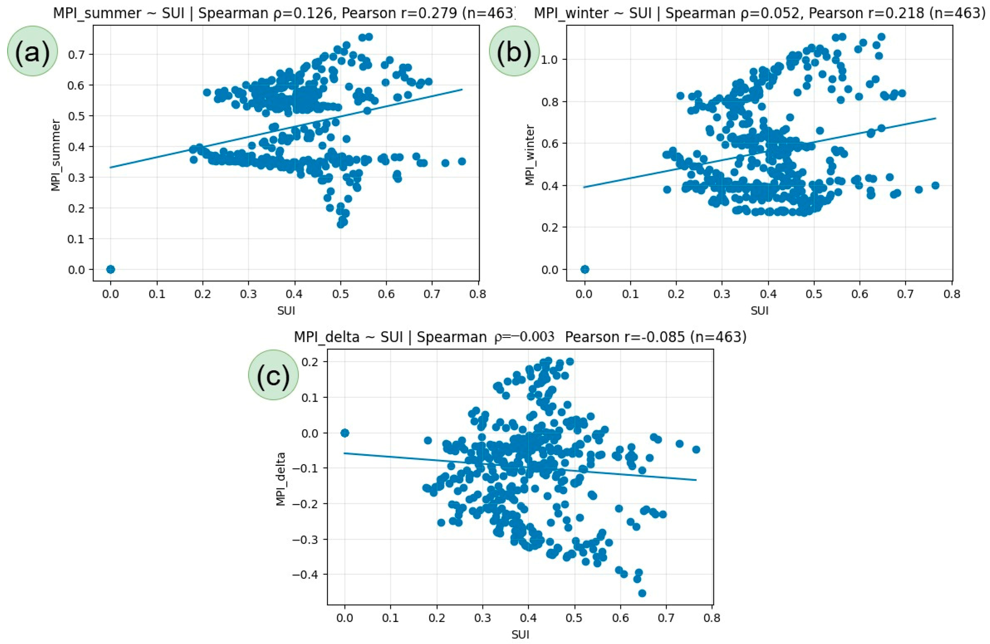
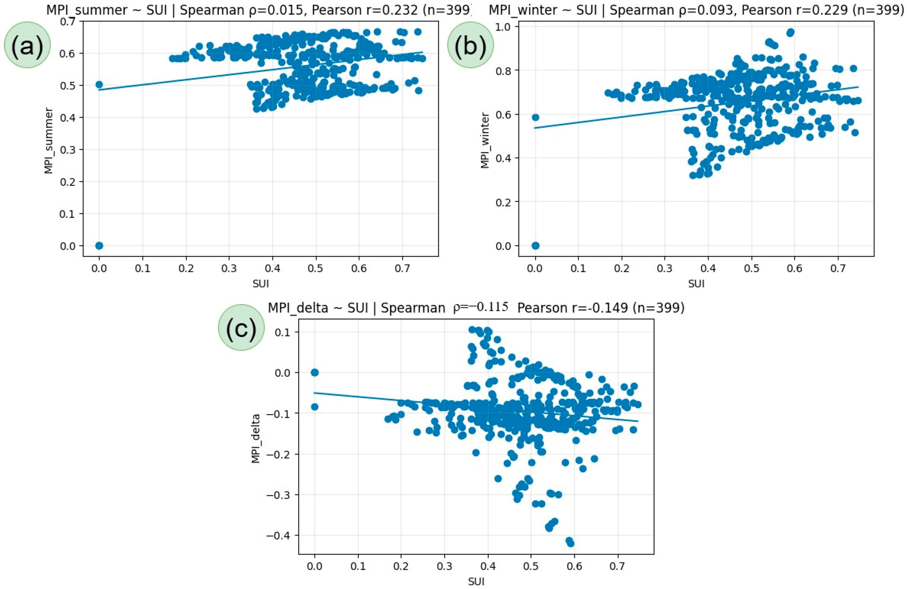
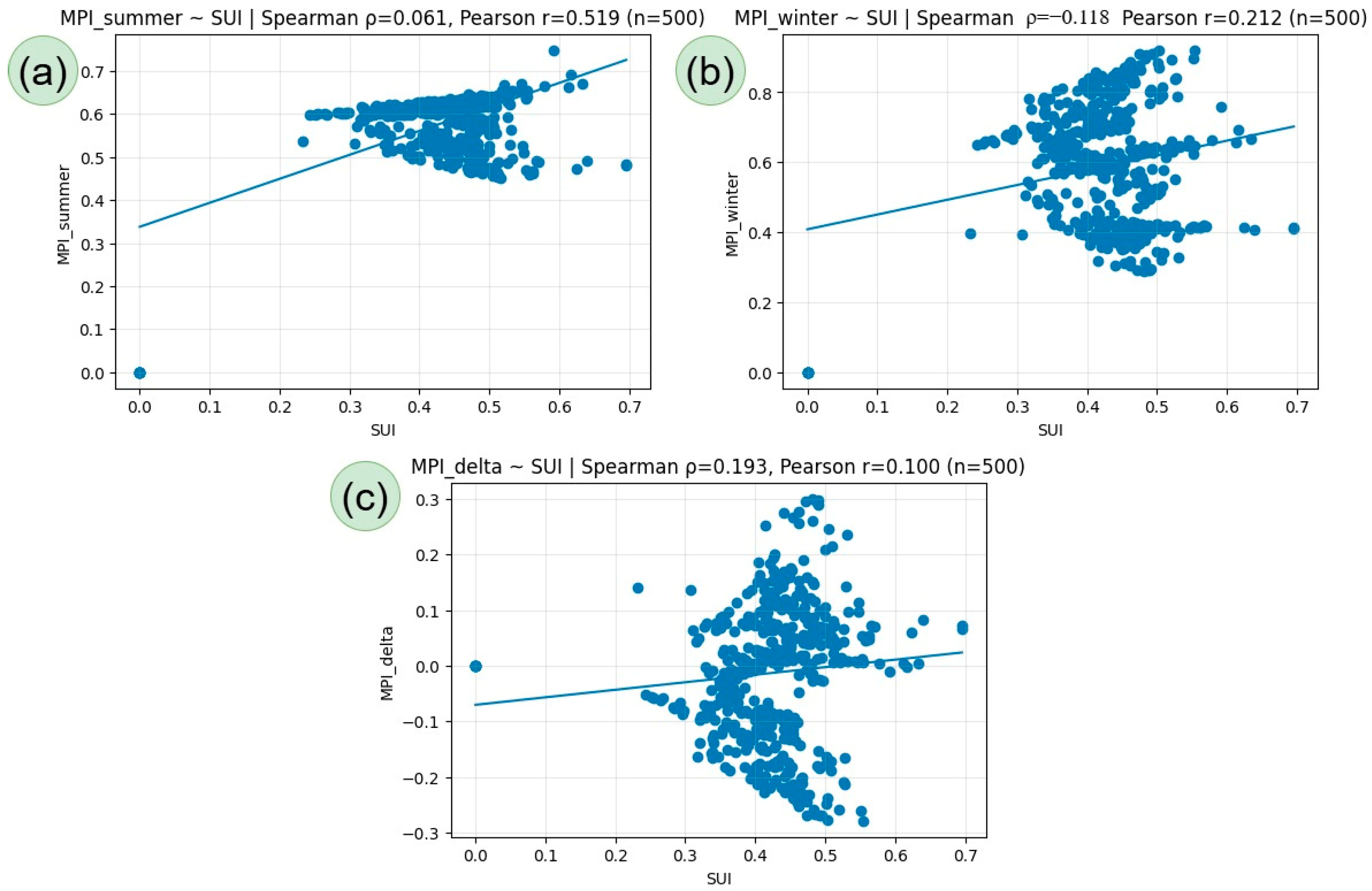
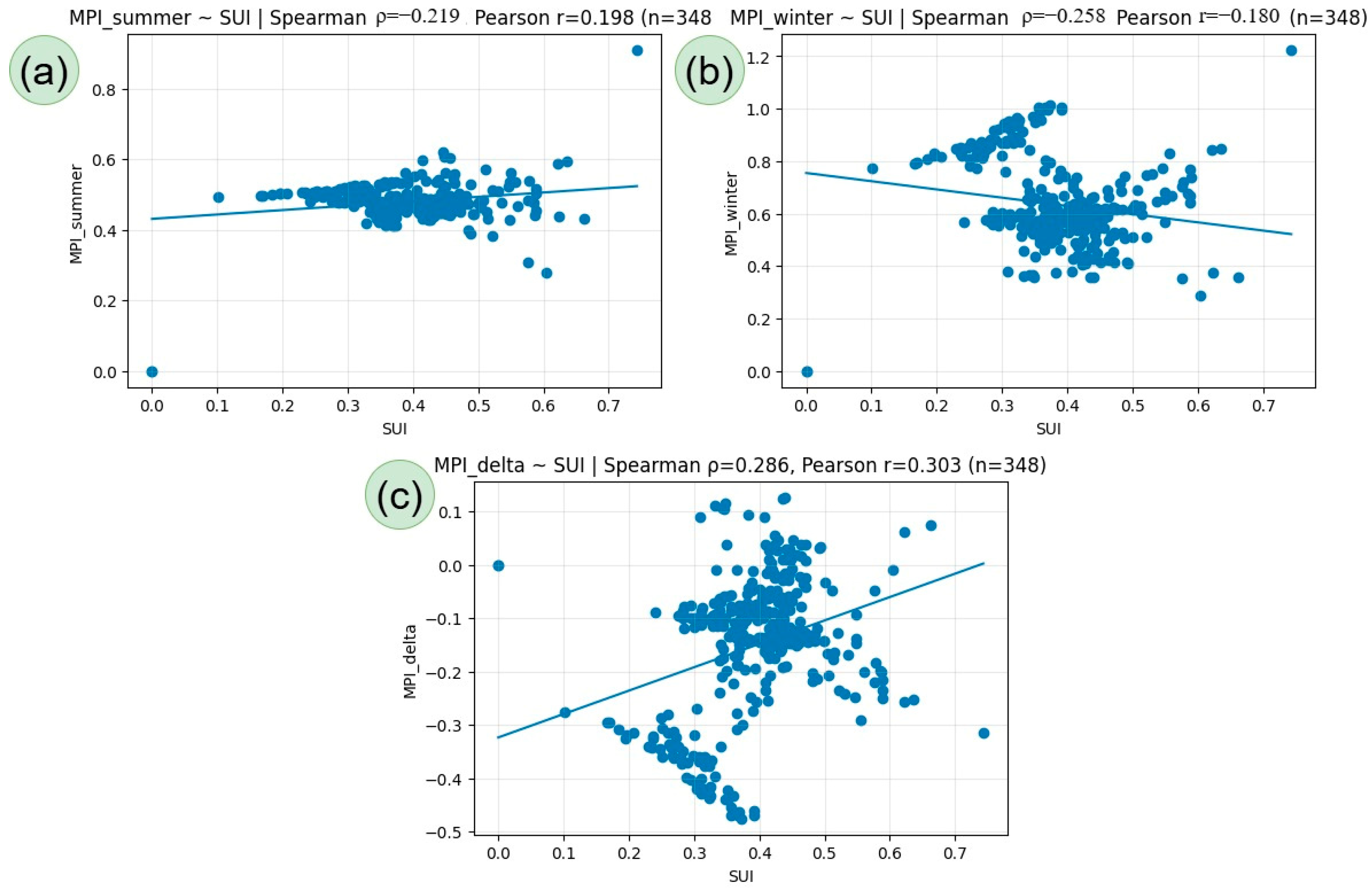
In the second stage, the relationship was examined at the pixel scale through random point sampling within each provincial boundary. These points were generated independently for each province and were used to extract co-located values from the SUI raster and the three composite pollution surfaces (${RMS}_{summer},{RMS}_{winter},∆MPI$) by means of the Extract Multi Values to Points tool. This procedure produced a province-specific tabular dataset in which SUI values and seasonal pollution values were linked at identical spatial locations. The primary statistical measure used in the analysis was Spearman’s rank correlation coefficient (ρ), selected because SUI is a normalized composite index and because the RMS and ΔMPI based variables do not guarantee normality or linearity. Spearman’s coefficient was therefore preferred as a more robust measure of monotonic association. Pearson’s correlation coefficient (r) was reported only as a secondary sensitivity-oriented measure to examine whether the observed relationships approximated a linear structure. All analyses were conducted separately for each province and for each composite pollution metric.

The point-based correlation analysis was designed as a complementary exploratory step rather than as the sole inferential basis of the SUI–pollution relationship. Its purpose was to evaluate the direction and relative magnitude of province-level association after extracting co-located raster values within each provincial boundary. Because raster-derived observations may retain spatial dependence, these correlation results should be interpreted cautiously and together with the class-based zonal statistics, which provide a more aggregated basis for comparing seasonal multi-pollutant burden across ordered SUI classes.

5. Results

5.1. SUI Surfaces as Tourism-Transport Pressure Contexts

Figure 4 presents the AHP-based, Fuzzy SIWEC-based, and final integrated SUI surfaces for the four study provinces. A first observation relevant to methodological interpretation is that the AHP and Fuzzy SIWEC outputs exhibit highly similar spatial tendencies in all provinces, despite minor differences in local intensity. This convergence indicates that the spatial structure of the results is not an artifact of a single weighting method; rather, the main suitability pattern remains stable across alternative expert-based weighting schemes. The final SUI maps, obtained through the averaging of the two weighted outputs, preserve the dominant spatial tendencies while providing a more balanced and consensus-oriented representation of tourism-transport suitability. Weight values are given in

Table 4. Comparative weight values of the sub-criteria obtained from the AHP and Fuzzy SIWEC methods.

Sub-Criteria	Weight Values		Sub-Criteria	Weight Values
	AHP	FSIWEC		AHP	FSIWEC
C1.1	0.0793	0.09208	C3.1	0.0801	0.08813
C1.2	0.1557	0.10788	C3.2	0.0668	0.07927
C2.1	0.0935	0.09338	C3.3	0.062	0.08899
C2.2	0.1737	0.11238	C4.1	0.0442	0.08590
C2.3	0.1496	0.10179	C4.2	0.0123	0.07178
C2.4	0.0828	0.07840

. The full AHP procedure is documented in File S1. Specifically, File S1 provides the expert-specific pairwise comparison matrices for all 11 sub-criteria, the derived priority vectors, and the associated consistency statistics (λmax, CI, and CR) for each expert. All calculated CR values remained below the commonly accepted threshold of 0.10, indicating an acceptable level of judgment consistency. These Supplementary Materials are provided to improve methodological transparency and reproducibility.

From a spatial perspective, the integrated SUI surfaces reveal that suitability is not distributed uniformly across provincial territories. Instead, high-SUI areas tend to cluster along coastal belts, major accessibility corridors, and destination-specific concentration zones, where tourism attraction, accommodation capacity, mobility infrastructure, and population intensity intersect. These areas should be interpreted as spatial contexts in which tourism- and transport-related activity is more likely to concentrate, and where interactions between visitor flows, local mobility demand, and resident presence become more pronounced. In this sense, the SUI maps do not directly represent air pollution; rather, they identify the underlying territorial structure within which environmental pressure and potential exposure are more likely to intensify.

Province-level differences are also clearly visible in Figure 4. In Antalya, high suitability is organized along a relatively continuous coastal axis, broadly reflecting the strong tourism-transport linkage between the main coastal settlements and the D400 corridor. Muğla displays a more fragmented and multi-nodal pattern, with suitability concentrating around major destination clusters such as Bodrum, Marmaris, and Fethiye. In Aydın, high-SUI areas are more selective and appear primarily along the Kuşadası-Didim coastal strip and its associated access structure. İzmir presents the most complex pattern, with multiple suitability cores emerging from the interaction of metropolitan transport functions, port-related activities, coastal tourism, and urban concentration. Collectively, these results suggest that tourism-transport suitability in coastal Türkiye is structured not only by tourism attractiveness itself, but also by the spatial organization of accessibility and population-related activity.

From an analytical standpoint, the SUI surfaces provide the common spatial reference layer for the subsequent comparison with the seasonal pollution indicators. Areas with higher SUI values do not automatically imply higher pollution; rather, they indicate where attraction, accommodation, accessibility, and population-related activity co-concentrate more strongly within the provincial setting. The subsequent pollution analysis therefore asks whether these higher-pressure contexts are associated with systematically different seasonal multi-pollutant patterns. In this sense, the SUI map functions as the explanatory spatial framework, while the RMS and ΔMPI surfaces function as the environmental outcome layers.

In this study, the final SUI surface was derived by taking the arithmetic mean of the AHP-based and Fuzzy SIWEC-based suitability maps. This step was not intended to suppress methodological differences, but to provide a single common reference surface for the subsequent linkage analysis with the seasonal multi-pollutant indicators. Importantly, the method-specific outputs were not concealed; rather, both AHP- and Fuzzy SIWEC-based maps are presented separately in Figure 4, allowing readers to visually assess their similarities and local differences. Since the two weighting approaches rely on different judgment structures, their separate presentation makes the effect of weighting variation explicit, whereas the integrated SUI serves as a consensus-oriented analytical surface for comparing suitability patterns with summer, winter, and ΔMPI pollution layers within a unified framework.

5.2. Seasonal Multi-Pollutant Composite Surfaces and ΔMPI

Figure 5 presents the RMS-based multi-pollutant composite surfaces for the summer and winter periods together with the signed interseasonal difference layer ($∆MPI={RMS}_{summer}-{RMS}_{winter}$) for each province. These maps constitute a central analytical output of the study because they move beyond pollutant-specific interpretation and provide a unified representation of the combined seasonal burden associated with seven normalized pollutant sub-indices. In methodological terms, the RMS framework improves interpretability by synthesizing pollutant-specific seasonal responses, which may differ in both magnitude and direction, into a single dimensionless metric. As such, the composite maps should not be read as simple substitutes for individual pollutant surfaces, but rather as integrative layers that make cross-provincial and cross-seasonal comparison more coherent.

A first general observation from Figure 5 is that the summer and winter RMS surfaces do not reproduce a uniform seasonal pattern across the four provinces. Instead, the composite burden varies by province in both level and spatial continuity. This finding is consistent with the overall conclusion of the study that air pollution in coastal tourism regions is shaped by province-specific seasonal dynamics rather than by a single common tourism-related pattern. In this respect, the RMS maps are analytically valuable precisely because they condense different and sometimes opposing pollutant behaviors into a single comparative surface.

The inter-seasonal contrast layer is particularly useful for interpretation because it makes seasonal directional change more visible than absolute burden surfaces alone. By construction, positive ΔMPI values indicate locations where the composite burden is relatively higher in summer, whereas negative values indicate winter dominance. However, these surfaces should be interpreted carefully. They do not identify a direct causal tourism effect; rather, they indicate where seasonal change in the composite pollution field becomes spatially visible and therefore where tourism-season-sensitive environmental dynamics may be more plausibly examined. This distinction is important because the broader results of the study show that the relationship between SUI and pollution is generally weak and context dependent, and that seasonal change offers a clearer signal in only some provincial settings.

The province-level differences in Figure 5 reinforce this interpretation. In Aydın, the Δ surface separates the direction and magnitude of seasonal change clearly and indicates that summer-related composite increases are not distributed homogeneously across the province, but instead emerge in selected attraction- and activity-oriented locations. This suggests that tourism-season effects in Aydın are spatially selective rather than province-wide, while winter conditions appear to sustain a broader composite burden across larger areas. In this sense, the RMS framework makes a dispersed seasonal signal more readable and offers a clearer basis for subsequent SUI-linked interpretation.

In Muğla, the RMS surfaces show a marked seasonal contrast in both level and spatial distribution. The summer surface is characterized more by localized clusters, whereas the winter surface reaches generally higher values and exhibits a more spatially continuous pattern. The Δ layer is therefore dominated by negative values over large parts of the province, indicating that the composite burden remains more strongly winter-oriented even in areas associated with high tourism intensity. At the same time, limited positive foci are still visible, showing that relative summer increases occur locally rather than systematically. This province-specific result suggests that the environmental signature of tourism seasonality in Muğla is selective and does not override the broader winter burden.

A broader implication of Figure 5 is that the seasonal difference layer is analytically more informative than absolute seasonal maps alone when the objective is to test whether tourism-season-related change becomes spatially detectable. The study’s overall findings support this reading by showing that Δ-based analyses provide a clearer signal in some provinces than direct comparison of summer and winter burden levels. Thus, the key contribution of the RMS and Δ surfaces lies not in proving a uniform tourism effect, but in revealing where and under what spatial conditions seasonal multi-pollutant burden becomes more clearly differentiated.

To maintain the readability of the main text, only the integrated suitability and composite pollution maps are presented in Section 5. The full set of spatial inputs used in the analysis, including the normalized maps of the 11 SUI sub-criteria for each province and the pollutant-specific seasonal sub-index surfaces derived through reference-based normalization, is provided in Files S2 and S3.

5.3. Class-Based and Point-Based Evidence on the SUI–Pollution Relationship

After the construction of the SUI surfaces and the derivation of the seasonal multi-pollutant composite layers, the relationship between the tourism-transport pressure-context surface and seasonal pollution burden was examined through two complementary analytical steps: class-based zonal statistics and province-level point-based correlation analysis. This combined design was adopted in order to move beyond visual map comparison and to evaluate whether areas characterized by similar suitability levels also exhibit systematically different composite pollution burdens. In methodological terms, the objective was not merely to show spatial overlap between SUI and RMS surfaces, but to determine whether the direction and magnitude of the tourism-season signal could be interpreted quantitatively through class summaries and correlation coefficients. These two analytical steps were designed to evaluate the expectations stated in the Introduction by examining both class-level consistency and point-based spatial association between the explanatory SUI surface and the seasonal pollution indicators.

5.3.1. Zonal Statistics as Class-Based Evidence

In the first stage, the SUI raster was classified into eight ordinal classes and used as the zoning framework for the ArcMap Zonal Statistics procedure. The value rasters were the seasonal multi-pollutant surfaces—namely, ${RMS}_{summer},{RMS}_{winter}$—and the seasonal contrast layer ($∆MPI or {RMS}_{∆}$, depending on notation). This step was introduced for three related reasons. First, it enabled the study to test whether composite pollution burden increases monotonically across higher SUI classes. Second, it made it possible to identify the SUI classes in which the seasonal contrast becomes more pronounced. Third, it established a fairer basis for interprovincial comparison by evaluating Antalya, Muğla, Aydın, and İzmir under comparable tourism-transport suitability conditions rather than through whole-province averages alone. The zonal summaries also reduce pixel-scale noise and therefore translate visually perceived spatial similarity into more interpretable class-level evidence.

From an interpretive standpoint, the zonal results provide an aggregated basis for assessing whether the upper SUI classes correspond to elevated multi-pollutant burden and whether seasonal change becomes more visible in those upper classes. The analytical framework treats this as a test of consistency between tourism-transport pressure and pollution burden rather than as direct evidence of causality. Where higher SUI classes coincide with increasing RMS or with positive Δ signals, the results support the interpretation that tourism-transport pressure may be spatially associated with increased environmental burden. Where this pattern is absent or weak, the results indicate that other seasonal and territorial drivers dominate the pollution field. In this sense, the zonal analysis is the bridge between the map-based results presented in the previous sections and the point-based correlation evidence discussed below.

5.3.2. Random Point Sampling and Province-Level Association Analysis

In the second stage, the relationship was evaluated at the pixel scale through random point sampling within each provincial boundary. Homogeneously distributed sample points were generated independently for Antalya, Muğla, Aydın, and İzmir, and the spatial design of these points is shown in Figure 6. For each point, values were extracted from the SUI raster and from the three composite pollution rasters (${RMS}_{summer},{RMS}_{winter}, \mathrm{a}\mathrm{n}\mathrm{d} ∆MPI$) using the ArcMap Extract Multi Values to Points tool. This procedure produced a province-specific tabular dataset in which SUI values and seasonal pollution values were linked at identical spatial locations, thereby allowing the SUI–pollution relationship to be tested statistically rather than inferred only from overlaid maps.

The choice of correlation metrics follows directly from the structure of the data. Because SUI is a normalized composite index derived from weighted criteria, and because the distributions of RMS and ΔMPI do not necessarily satisfy linearity or normality assumptions, Spearman’s rank correlation coefficient (ρ) was used as the primary measure of association. Spearman’s coefficient is better suited to identifying monotonic relationships under these conditions. Pearson’s correlation coefficient (r) was reported as a secondary, sensitivity-oriented indicator to assess whether the relationship approximates a linear form. This combination does not assume that the SUI–pollution relationship is linear; rather, it allows the study to compare monotonic and approximately linear tendencies in parallel.

Random points were automatically generated in ArcMap within each provincial boundary and used to extract co-located SUI and seasonal pollution values from the raster surfaces. Sample sizes were 463 for Antalya, 399 for Muğla, 500 for Aydın, and 348 for İzmir. This step was designed to provide province-specific distributed raster observations for exploratory association analysis, rather than a formally area-weighted sampling scheme. Spatial autocorrelation was not explicitly modelled and is therefore recognized as a limitation when interpreting the resulting correlation coefficients. A fixed random seed was not retained during the automated point-generation step in ArcMap. Therefore, the exact point locations are not strictly reproducible point by point, although the same sampling logic, provincial boundaries, and sample sizes can be re-applied. This should be interpreted as a reproducibility limitation of the exploratory point-based correlation analysis rather than of the overall GIS framework.

5.3.3. Interpretation of Province-Level Results

The province-level results summarized in

Table 5. Province-based exploratory correlation results between SUI and the seasonal multi-pollutant composite indicators.

Province	n	Metric	Spearman ρ	${\mathit{\rho }}^2$	p-Value	Pearson r
Antalya	463	${MPI}_{summer}$	0.126 *	0.016	<0.01	0.279
		${MPI}_{winter}$	0.052	0.003	0.267	0.218
		ΔMPI	−0.003	0.000	0.948	−0.085
Muğla	399	${MPI}_{summer}$	0.015	0.000	0.764	0.232
		${MPI}_{winter}$	0.094	0.009	0.061	0.229
		ΔMPI	−0.115 *	0.013	0.021	−0.149
Aydın	500	${MPI}_{summer}$	0.061	0.004	0.174	0.519
		${MPI}_{winter}$	−0.118 **	0.014	0.008	0.212
		ΔMPI	0.193 ***	0.037	<0.001	0.100
İzmir	348	${MPI}_{summer}$	−0.219 ***	0.048	<0.001	0.198
		${MPI}_{winter}$	−0.258 ***	0.067	<0.001	−0.180
		ΔMPI	0.286 ***	0.082	<0.001	0.303

Statistical significance levels are indicated as follows: * p < 0.05, ** p < 0.01, *** p < 0.001.

and illustrated in Figure 7, Figure 8, Figure 9 and Figure 10 indicate that the relationship between SUI and composite pollution burden is generally weak and context dependent, which is fully consistent with the overall logic of the study. This weak and context-dependent structure is itself informative, as it indicates that tourism-transport pressure does not translate into pollution burden through a single uniform spatial mechanism across all provincial contexts. The correlation analysis was not designed to prove a strong deterministic link, but to evaluate whether the spatial pressure field represented by SUI aligns, even weakly, with seasonal composite pollution surfaces once those surfaces are reduced to comparable point-based observations. The province-level correlation coefficients should therefore be interpreted as exploratory association measures within the provincial spatial framework, rather than as fully spatially corrected inferential statistics. This general pattern of weak but interpretable association is likewise reflected in the overall results and discussion. In interpretive terms, the class-based zonal statistics provide the primary aggregated quantitative basis for evaluating whether seasonal burden varies systematically across ordered SUI levels, while the point-based correlations serve as secondary evidence supporting directional and comparative reading.

In Antalya, the summer relationship is weakly positive (ρ = 0.126, p < 0.01), whereas the winter relationship is negligible and the seasonal-difference relationship is effectively absent. The corresponding descriptive ρ² value for summer is 0.016, indicating that the SUI is associated with only a very small fraction of the ranked spatial variability in the seasonal pollution signal. Read together with the SUI and RMS maps, this suggests that high-suitability coastal and corridor zones in Antalya may exhibit only a limited summer-oriented increase in composite burden, and that this weak pattern does not remain strong enough to define the province-scale inter-seasonal contrast. In other words, Antalya’s tourism-transport suitability shows only a modest spatial association with summer burden, while the broader pollution field remains shaped mainly by additional factors beyond tourism-season intensity. This interpretation is consistent with the provincial discussion in the result section, which emphasizes Antalya’s strong coastal continuity but does not imply a dominant or exclusive tourism effect on pollution.

In Muğla, the summer and winter correlations are close to zero, whereas the ΔMPI relationship is weakly negative (ρ = −0.115, p = 0.021). The corresponding descriptive ρ² value is 0.013, indicating that the SUI is associated with only a very small fraction of the ranked spatial variability in the seasonal-difference signal. This pattern suggests that, even in a province where tourism intensity is structurally high, the seasonal composite burden does not increase systematically with higher SUI values. Instead, the negative Δ signal indicates that many of the high-SUI zones remain more closely associated with winter-dominant burden than with summer intensification. When read together with the RMS and Δ maps, this supports a cautious interpretation in which Muğla’s tourism-related environmental signature appears selective and spatially fragmented rather than uniformly summer-driven.

In Aydın, the summer relationship is weak and statistically non-significant, whereas the winter relationship is weakly negative (ρ = −0.118, p = 0.008) and the seasonal-difference relationship is weakly positive (ρ = 0.193, p < 0.001). The corresponding descriptive ρ² value for ΔMPI is 0.037, indicating that the SUI is associated with only a small fraction of the ranked spatial variability in the seasonal-difference signal. Within the present framework, this pattern is more informative than the absolute seasonal relationships because it suggests that the tourism-season signal is more visible in the inter-seasonal contrast. In other words, a direct summer-versus-SUI comparison would understate the relationship, whereas the seasonal-difference metric indicates that higher-suitability zones tend to be associated with relatively stronger summer-oriented change. At the same time, the magnitude of this association remains limited and should therefore be interpreted as a modest contextual signal rather than as a strong provincial-scale relationship. This is aligned with the study’s broader argument that Δ-based metrics may be more informative than absolute seasonal levels in selected provincial contexts.

In İzmir, the absolute seasonal relationships are weakly negative in both summer (ρ = −0.219, p < 0.001) and winter (ρ = −0.258, p < 0.001), whereas the ΔMPI relationship is the strongest positive association observed in the study (ρ = 0.286, p < 0.001). However, the corresponding descriptive ρ² value is 0.082, indicating that the SUI is associated with only a small fraction of the ranked spatial variability in the seasonal-difference signal. This contrast nonetheless remains informative in comparative terms. It suggests that the metropolitan and background pollution structure of İzmir weakens the direct association between SUI and absolute seasonal burden, while the inter-seasonal change metric is relatively more effective in identifying a suitability-related signal. In practical terms, İzmir illustrates why a direct “high SUI = high pollution” interpretation would be too simplistic: the absolute burden field reflects a more complex urban system, whereas the seasonal-difference layer appears better able to indicate where summer-oriented intensification becomes spatially more coherent. At the same time, the magnitude of this association remains limited and should not be interpreted as evidence of a strong provincial-scale relationship.

The main value of the point-based correlation analysis lies in how it complements the preceding spatial analyses. The SUI maps identify where tourism-transport pressure is likely to concentrate; the RMS and Δ maps identify where seasonal multi-pollutant burden is elevated or changes directionally across seasons; the zonal statistics show whether those burdens intensify across higher SUI classes; and the correlation analysis adds a pixel-scale indication of the direction and relative magnitude of that relationship. In this respect, Table 5 and Figure 7, Figure 8, Figure 9 and Figure 10 should not be interpreted in isolation. Rather, they represent the final quantitative layer of an integrated spatial argument. At the same time, the correlation coefficients remain small in effect size, indicating that tourism-transport suitability is associated with only a limited fraction of the ranked spatial variability in the pollution indicators within the present exploratory framework.

Taken together, the weak correlations indicate that the relationship is mediated by meteorology, topography, background urban activity, and province-specific source structures. The study therefore supports a cautious conclusion: within the analytical framework adopted here, the SUI–pollution relationship is weak but interpretable, yet not strong enough to justify a simplistic deterministic reading. The most informative signal emerges not from absolute seasonal maps alone, but from the combined reading of SUI surfaces, RMS/Δ surfaces, zonal summaries, and exploratory province-level rank correlations.

The relationship examined in this study should not be interpreted as a test of direct causal or flow-based tourism impact on pollution. Since the SUI represents a spatial suitability and pressure-context surface rather than an observed traffic, emission, or tourism-flow metric, the expected relationship with pollution is not necessarily strong in a deterministic sense. Instead, the analytical objective is to examine whether areas characterized by stronger tourism-transport context tend to display systematically different seasonal multi-pollutant patterns when compared across the same provincial spatial framework. In this sense, the study tests an empirical spatial association, or structured spatial co-occurrence, rather than a direct causal relationship. This also helps explain why the observed correlations are generally weak: air pollution patterns are shaped not only by tourism-related context, but also by meteorology, topography, background urban activity, and province-specific source structures.

6. Discussion

6.1. Seasonal Contrast as a More Informative Lens than Absolute Seasonal Burden

The results suggest that the relationship between tourism-transport pressure and air pollution becomes more interpretable when examined through seasonal contrast, rather than through absolute seasonal burden alone. The summer and winter composite surfaces remain shaped by multiple overlapping drivers, including winter heating emissions, atmospheric stability, photochemical ozone formation, coastal–inland meteorological gradients, and province-specific urban source structures. For this reason, the signed seasonal-difference layer $(∆MPI={MPI}_{summer}-{MPI}_{winter})$ provides a more focused basis for interpretation, as it reveals where the composite burden changes directionally between tourism-intensive and low-tourism periods rather than merely showing where pollution is high in absolute terms. This point aligns with the study’s central contribution; namely, that the tourism–pollution relationship becomes more analytically meaningful when interpreted through seasonal differentiation and provincial context rather than through absolute burden levels alone.

This interpretation is fully consistent with the broader empirical conclusions of the study. The results indicate that the SUI–pollution relationship is generally weak and context dependent, that winter burden remains dominant in many areas despite the concentration of tourism in summer, and that the inter-seasonal layer provides a clearer signal in some provinces than the absolute summer or winter composites. In other words, the present findings suggest that tourism-season effects are more plausibly examined through relative spatial change than through absolute burden levels alone.

This result refines, rather than contradicts, the tourism-air quality literature reviewed in this work. Ref. [16] showed that tourism intensity can influence PM10 in Mallorca, while Zeng et al. (2021) [20] reported that tourism development can affect urban air pollution under different infrastructural conditions. Ref. [19] similarly found measurable coupling between tourism economy and air quality at the provincial scale. However, much of that literature operates either through single-pollutant analysis or through aggregate destination-level indicators. The present study reaches a more cautious and spatially nuanced conclusion: once tourism-transport pressure is modelled as a continuous GIS surface and pollution is represented through a multi-pollutant seasonal framework, the relationship remains detectable but weak, heterogeneous, and more interpretable through interseasonal contrast than through absolute seasonal levels. This position is also consistent with the broader literature framework, which treats the Δ layer as a methodologically important tool for distinguishing the tourism-season signal from broader seasonal pollution dynamics.

The province-level findings reinforce this interpretation. In Aydın and İzmir, the ΔMPI relationships are more informative than the absolute summer surfaces, indicating that high-suitability zones tend to be associated with relatively stronger summer-oriented change even where absolute pollution remains influenced by non-tourism sources. In Muğla, by contrast, the predominantly winter-oriented burden suggests that seasonal tourism pressure does not override broader winter drivers. Thus, the study does not support a uniform “tourism raises summer pollution everywhere” narrative; rather, it suggests that tourism-season-related environmental signals are spatially selective and mediated by local context.

6.2. RMS as a Response to the Limitations of Single-Pollutant Interpretation

A second methodological contribution of the study concerns the use of the Root Mean Square (RMS) framework to integrate seven normalized pollutants into a single multi-pollutant metric. This choice is particularly useful because the results show that pollutant-specific seasonal behavior does not move in a single common direction. Some pollutants exhibit stronger winter patterns, while others become more prominent in summer. Under such conditions, reliance on a single pollutant can generate contradictory interpretations. A winter-dominant PM-based reading and a summer-sensitive ozone-based reading may coexist in the same province, making it difficult to interpret the overall seasonal burden in a coherent way.

The RMS framework addresses this problem by converting pollutant-specific sub-indices into a common dimensionless surface while retaining the stronger contribution of relatively high local values. This is why the study found that RMS maps improved interpretability by synthesizing pollutant-specific and sometimes opposing seasonal tendencies into a single metric. In this sense, the RMS framework provides a more coherent basis for reading compound seasonal burden than single-pollutant surfaces alone. However, this interpretive advantage should not be confused with full absolute cross-provincial equivalence. Because the normalization strategy combines fixed WHO-based thresholds with province- and season-specific P95 references for NO and NOx, RMS values should be read as reference-normalized relative burden indicators within the analytical framework of the study rather than as fully standardized cross-provincial quantities. One methodological advantage of the RMS approach is that it reduces the risk of overgeneralization based on a single pollutant.

This result aligns well with the spatial and seasonal air pollution literature reviewed in this study. Studies such as [6,7,25] all emphasize that air pollution is both spatially heterogeneous and seasonally variable, while [24] highlights the value of spatially explicit transport-emission mapping for environmental interpretation. The present study extends that logic by showing that, in tourism-intensive coastal regions, the analytical challenge is not only spatial variability, but also the need to interpret compound seasonal burden in a way that can be meaningfully related to a pressure surface such as SUI.

The discussion is also consistent with the tourism-side literature reviewed in this work. Work on tourism carbon footprints and transport emissions, including studies such as [3,12,47], shows that tourism-related environmental burden is multi-component and not reducible to one single source or indicator. In the present study, the same logic appears at the air pollution level: the tourism–environment relationship is not meaningfully represented through one pollutant alone. Instead, a multi-pollutant framework is needed to capture the spatial signature of cumulative seasonal burden.

6.3. Why the SUI–Pollution Relationship Remains Weak but Meaningful: Background Controls, Scale Effects, and Temporal Mismatch

A central result of the study is that the SUI–pollution relationship remains weak, whether interpreted through class-based zonal statistics or through province-level point correlations. This pattern is consistent with the multi-causal structure of air pollution in coastal regions, where pollution levels are shaped not only by tourism-related mobility, but also by winter heating, metropolitan activity, industrial and port-related emissions, atmospheric stability, topographic modulation, and coastal meteorology. Under such conditions, a strong deterministic relationship between tourism-transport suitability and pollution would be analytically unlikely. The absence of a strong and spatially uniform relationship across all four provinces is therefore informative in itself, because it indicates that the tourism-transport signal becomes visible only under certain seasonal and provincial conditions rather than through a single common mechanism.

The empirical results support this reading. Across the four provinces, the observed relationship remains weak and context dependent, and the zonal summaries do not show a monotonic increase in composite burden across higher SUI classes in every case. This suggests that tourism-transport pressure leaves a spatial trace, but that trace is partial, mediated, and province specific rather than dominant and uniform. Within the present framework, the tourism-transport signal is therefore better understood as contingent on seasonal and territorial context than as a common province-scale mechanism.

A further explanation lies in the relative dominance of background controls over tourism-related signals. In coastal provinces, pollution fields may be governed more strongly by atmospheric stability, boundary-layer structure, coastal–inland air exchange, winter heating emissions, and topographically constrained accumulation patterns than by tourism-related mobility alone. Under such conditions, tourism effects do not necessarily disappear, but they may become analytically secondary within the broader pollution field. This is particularly plausible when the composite burden is shaped by multiple coexisting sources whose spatial influence is wider and more persistent than the localized pressure associated with tourism activity. For this reason, the weak relationship identified in the present study should not be interpreted as the absence of a tourism-related effect, but rather as evidence that such an effect operates within a wider environmental system dominated by stronger background controls in some provincial contexts.

One possible reason why the expected relationship does not emerge more strongly may be the spatial scale of the analysis itself. Although the study is conducted at the provincial level, many of the processes it seeks to capture, such as tourist mobility, traffic congestion, and localized emissions, are inherently fine-scale phenomena. In practice, these processes tend to concentrate in specific coastal strips, destination clusters, transfer corridors, urban service centers, and high-demand nodes rather than being distributed uniformly across an entire province. When such localized tourism-related signals are evaluated against province-wide interpolated multi-pollutant surfaces, their effect may become spatially diluted by broader background pollution processes operating at larger scales. In the present case, this means that a tourism-related signal may still exist, but may remain visible only in selective zones or through inter-seasonal contrast rather than appearing as a strong and uniform provincial-scale association. This scale mismatch therefore provides an important explanation for why the observed relationship is weak, while still remaining analytically meaningful.

A related issue concerns temporal mismatch between tourism peaks and pollution dynamics. Tourism demand and associated mobility generally intensify during the summer season, whereas the highest absolute burden for several pollutants may emerge in winter because of domestic heating, stagnant atmospheric conditions, and reduced dispersion capacity. Even during summer, pollutant concentrations may be shaped by photochemical behavior, background urban traffic, and local meteorological processes that do not correspond directly to tourism intensity. For this reason, a strong alignment between the SUI and the absolute summer or winter burden surfaces should not be expected a priori. The present findings support this interpretation, since the seasonal-difference layer provides a clearer and more interpretable signal in some provinces than the absolute seasonal composites. This suggests that tourism-related effects may be better captured through inter-seasonal contrast than through absolute burden levels alone.

This finding also resonates with the literature reviewed in this study. Ref. [20] reported that tourism’s effect on urban air pollution is moderated by infrastructure conditions, while refs. [31,48] showed that environmental burden often reflects unequal spatial exposure conditions rather than uniform sectoral effects. Similarly, studies such as [26,49,50] underline that traffic, infrastructure, urban form, and topographic or ecological context can reshape pollution patterns independently of tourism demand. The present study is therefore consistent with this broader body of work: tourism-transport pressure matters, but its effects emerge within a crowded field of other controlling mechanisms rather than in isolation.

The province-level results illustrate this complexity particularly well. Antalya exhibits only a weak positive summer relationship, suggesting that strong coastal tourism continuity does not automatically translate into a strong province-scale pollution response. Muğla’s weak negative Δ association indicates that winter-dominant burden remains important even in a strongly tourism-oriented province. Aydın offers one of the clearest examples of why the Δ layer matters, because the summer-only relationship remains weak whereas the inter-seasonal contrast becomes more interpretable. İzmir presents the most complex structure: the metropolitan background weakens the direct relationship with absolute seasonal burden, yet the ΔMPI relationship is the strongest positive signal in the study. These results support a cautious but meaningful conclusion: the tourism-transport signal is not absent, but it is only visible when interpreted together with seasonality and spatial context.

Taken together, these results show that the weak and context-dependent SUI–pollution relationship is not inconclusive, but analytically informative. The key implication is that tourism-related environmental pressure in coastal provinces should not be expected to produce a uniform pollution response across all settings or all seasons. Instead, its detectability depends on the interaction between localized tourism pressure, broader background emissions, meteorological regulation, topographic structure, and the temporal alignment between activity peaks and pollution formation processes. In this respect, the main contribution of the present study lies in revealing why the tourism-transport signal emerges only conditionally and why seasonal contrast offers a more meaningful interpretive lens than absolute burden alone in selected provincial contexts.

This interpretation should also be read with methodological caution. In the present study, the point-based correlations are not treated as fully spatially corrected inferential tests, but as exploratory province-level association measures that complement the class-based zonal summaries and the broader map-based reading. Accordingly, the analytical value of the correlation results lies more in their directional consistency and comparative contribution across provinces than in strict significance interpretation alone.

6.4. What Zonal Statistics Add Beyond Visual Map Comparison

The role of zonal statistics in the study deserves explicit emphasis. One of the risks in GIS-based tourism–pollution studies is to stop at visual overlay and infer relationships from apparent spatial coincidence. The present study deliberately moved beyond that level. By dividing the SUI surface into eight classes and summarizing RMS and Δ values within those classes, the analysis transformed SUI from a descriptive pressure map into a quantitative explanatory framework. As this study explicitly states, the major contribution of the zonal step is that it limits the “visual similarity” argument and makes class-level differences in pollution burden readable and reportable.

This step strengthens the interpretation of the SUI maps by moving beyond visual overlap alone. The SUI surfaces identify where tourism attractiveness, accommodation structure, accessibility, and population exposure context overlap. The RMS maps identify where multi-pollutant burden is elevated or changes seasonally. Zonal statistics then show whether that burden becomes more pronounced in higher suitability classes. The fact that this pattern is not monotonic in every province is itself a finding: it demonstrates that the SUI–pollution relationship is spatially structured but not uniformly scalable. In other words, tourism-related pressure is one part of the environmental system, but not the only one.

This class-based perspective also connects the study to environmental health and environmental justice concerns already present in the literature review. From both planning and justice/exposure perspectives, zonal comparison provides an analytically meaningful basis for interpretation. That framing is strengthened by studies such as [4,51,52], which demonstrate that traffic-related pollution burdens carry measurable health consequences, and by [31], which shows that environmentally unequal exposure can emerge around tourism-heavy urban systems. Within that broader context, the zonal results of the present study are valuable not because they identify epidemiological effects directly, but because they identify where environmental pressure and compound burden are more likely to overlap spatially.

6.5. Planning Implications and Future Research Directions

The present findings suggest that planning implications should not be framed through a deterministic assumption that tourism-transport suitability mechanically produces higher pollution. Rather, the results support a more conditional reading in which tourism-related signals interact with broader atmospheric, urban, and topographic controls. From a policy perspective, this implies that decarbonization and environmental management in coastal tourism regions should not rely on generalized seasonal assumptions alone. Instead, low-carbon transition strategies should be built around spatial selectivity, seasonal differentiation, and stakeholder coordination across sub-provincial contexts. In practical terms, this points to the need for stronger alignment between destination management organizations, local operators, and public authorities in the design of mobility management, visitor communication, environmental monitoring, and season-specific mitigation priorities. Such an interpretation is consistent with recent work emphasizing that sustainability outcomes in coastal tourism systems depend not only on technical measures, but also on integrated governance, strategic communication, and the coordinated involvement of multiple destination actors.

More specifically, the present results support three practical directions for tourism-sector decarbonization in coastal regions. First, mobility-related measures should prioritize the reduction and reorganization of seasonal transport pressure in high-suitability coastal and corridor zones through better public transport integration, active mobility support, low-impact destination circulation, and season-sensitive demand management. Second, accommodation- and service-related mitigation should focus on context-specific operational efficiency, energy management, and low-carbon facility practices, particularly in areas where tourism intensity and environmental burden co-concentrate. Third, governance-oriented strategies should strengthen coordination between destination management organizations, local authorities, and tourism operators so that visitor communication, environmental monitoring, and seasonal planning are aligned within the same low-carbon destination framework. In this sense, the study does not claim to provide a universal decarbonization model; rather, it offers a spatial basis for identifying where differentiated and context-sensitive low-carbon interventions are more likely to be needed.

Several limitations should nonetheless guide interpretation. The analysis is based on a relatively short observational window, which restricts inter-annual comparison. Station density varies across provinces, which may affect the stability of the interpolation surfaces. IDW provides a transparent and widely used method for surface generation; however, it does not account for topographic channeling or atmospheric transport processes. Finally, the SUI framework captures the spatial structure of tourism-transport pressure, but not dynamic demand-side indicators such as real-time traffic flows, airport passenger peaks, or accommodation occupancy. These limitations are already acknowledged in this study and point directly toward future research priorities: multi-year monitoring, dynamic mobility indicators, uncertainty-aware interpolation, remote sensing support, and direct health outcome integration would all deepen the explanatory power of the framework. The spatial distribution of the air quality monitoring stations used in this study was determined by the national monitoring network rather than by the authors, and station density is not uniform across the four provinces. For this reason, IDW was adopted as a practical and transparent interpolation method suitable for generating comparable provincial pollution surfaces within the available monitoring framework. However, the authors acknowledge that no formal sensitivity assessment or comparison with alternative interpolation methods, such as kriging, was conducted in the present study. This should be considered a methodological limitation, particularly in provinces with sparser station coverage, where interpolation uncertainty may be higher. Future research should therefore compare IDW-based outputs with alternative geo-statistical approaches and include uncertainty-oriented validation procedures to strengthen the robustness of the pollution surfaces.

An additional limitation concerns the use of raster-derived point samples in the correlation analysis. Because such observations may retain spatial autocorrelation, the reported Spearman and Pearson coefficients should be interpreted as exploratory association measures rather than fully spatially independent inferential statistics. Future studies should therefore incorporate Moran’s I-based diagnostics, spatial filtering procedures, or other spatially informed modeling strategies in order to strengthen the robustness of the statistical association analysis.

A further limitation concerns the absence of a full land-use buildout or zoning-sensitive development scenario analysis. Buildout analysis is commonly used to estimate maximum development under current zoning and environmental constraints and to examine how land-use patterns may evolve under different regulatory environments and development trajectories [53]. The present GIS framework identifies where tourism-transport pressure-context and seasonal pollution burden become spatially comparable under observed current conditions, but it does not simulate how alternative regulatory environments, maximum development potential, or different rates of land-use change might reshape future transport demand and air-pollution burdens. In this respect, the study should not be interpreted as a buildout-based urban growth assessment. Future research could therefore integrate buildout analysis, zoning-sensitive land-use scenarios, or urban growth modeling in order to examine how evolving development patterns may alter tourism-related mobility pressure and associated environmental burdens over time.

At the same time, these implications should be interpreted with caution. The analysis is based on a relatively short observational window, and station density varies across provinces. IDW was adopted as a practical interpolation method, but no formal sensitivity assessment or comparison with alternative geo-statistical approaches was conducted, which may increase interpolation uncertainty in provinces with sparser monitoring coverage. In addition, the hybrid normalization framework, which combines fixed WHO-based thresholds with province- and season-specific P95 references for NO and NOx, limits the extent to which absolute RMS values can be interpreted as fully equivalent across provinces. The expert panel used in the weighting stage was also relatively small and discipline-specific, and did not include specialists from air quality, atmospheric science, tourism economics, or environmental health. Moreover, the criterion hierarchy was reviewed through a single-round expert procedure rather than a formal Delphi-based or consensus-driven validation process. For these reasons, the study should be interpreted as a comparative and exploratory spatial framework rather than as a fully standardized or universally generalizable decision model.

7. Conclusions

This study developed an integrated GIS-based framework to examine the spatial relationship between tourism-transport pressure-context and seasonal multi-pollutant air pollution across four major coastal provinces of Türkiye. By combining a multi-criteria Tourism-Transport Suitability Index (SUI), seasonal pollutant interpolation, reference-based normalization, RMS-based multi-pollutant aggregation, seasonal difference mapping, class-based zonal statistics, and province-level association analysis, the study moved beyond both single-pollutant interpretation and single-season comparison. In this way, it provided a comparative provincial framework for evaluating whether tourism-transport pressure-context and air pollution dynamics co-vary under different seasonal conditions.

The main goal of the study was not to prove a direct and universal tourism-driven pollution effect, but to evaluate whether areas characterized by stronger tourism-transport pressure-context also display systematically different seasonal multi-pollutant patterns across coastal provinces. The results show that this relationship is generally weak, spatially selective, and context-dependent rather than uniform or deterministic. Higher suitability does not automatically correspond to uniformly higher pollution burden. Instead, the tourism-transport signal becomes interpretable only under certain provincial and seasonal conditions, and in some cases is more clearly revealed by the seasonal-difference layer than by absolute summer or winter burden alone. In particular, the clearer ΔMPI patterns observed in Aydın and İzmir indicate that inter-seasonal contrast provides a more informative analytical lens than absolute seasonal burden when examining whether tourism-season-sensitive spatial structures become visible.

A second important conclusion is methodological. The SUI surfaces show that tourism-transport pressure is not territorially uniform, but tends to concentrate along coastal belts, destination clusters, and corridor-like accessibility structures. At the same time, the RMS-based composite framework improves the interpretation of seasonal air pollution by integrating pollutant-specific and sometimes opposing seasonal behaviors into a single dimensionless metric. Taken together, these results show that the tourism–pollution relationship in coastal provinces cannot be meaningfully interpreted through single pollutants, single seasons, or visually inferred map overlap alone. Rather, it should be examined through a comparative framework capable of capturing spatial selectivity, seasonal mediation, and province-specific background controls.

From a planning perspective, the findings do not justify generalized seasonal assumptions or a simple reading in which tourism-transport suitability mechanically determines air pollution. Instead, they point toward differentiated and context-sensitive decarbonization priorities within coastal tourism systems. More specifically, three practical directions emerge. First, mobility-related strategies should focus on reducing and reorganizing seasonal transport pressure in high-suitability coastal and corridor zones through stronger public transport integration, low-impact destination circulation, and season-sensitive demand management. Second, accommodation- and service-related mitigation should prioritize energy efficiency and low-carbon operational practices in areas where tourism intensity and environmental burden are more likely to co-concentrate. Third, governance-oriented strategies should improve coordination between destination management organizations, local authorities, and tourism operators so that visitor communication, environmental monitoring, and seasonal planning are aligned within a shared low-carbon destination framework. In this respect, the contribution of the study lies less in demonstrating a universally strong tourism–pollution linkage than in providing a comparative spatial basis for more targeted low-carbon tourism planning, locally adapted monitoring, and improved coordination between tourism development and environmental governance.

Several directions for future research emerge from these findings. Extending the analysis to multi-year datasets would help to determine whether the observed seasonal-difference patterns remain stable across time or are shaped by year-specific meteorological conditions. Alternative interpolation methods and uncertainty-oriented spatial validation could further strengthen the robustness of the pollution surfaces. In addition, incorporating dynamic mobility and tourism-demand indicators, such as traffic counts, airport passenger volumes, or accommodation occupancy, would improve the temporal sensitivity of the framework and allow the tourism-transport pressure–pollution relationship to be examined with greater explanatory depth.