Comparison of Local Spatial Deviation Indicators with Their Associated Tests: Evidence from Simulations and Applied Cases

Abstract

Currently, two kinds of local spatial deviation indicators, namely local spatial heteroscedastic statistics and local spatial variance, with their associated tests have been proposed for estimating and inferring the characteristics of a spatial process at the second-order moment level, which is of wide potential application in spatial data analysis. Nonetheless, the performance of the indicators with their associated tests remains to be systematically investigated. Due to their mixed application orientations and the difficulty in theoretically comparing their performance, we design proper simulation experiments to assess their performance in estimating the variance function of a spatial process and detecting the local spatial heteroscedasticity and the boundaries of spatial homogeneous clusters. Some worthwhile findings are obtained and their performance from different application orientations is clarified. Based on the findings, two real-life spatial datasets are analyzed to demonstrate the applications of the indicators with their associated tests.

1. Introduction

Spatial autocorrelation and spatial heteroscedasticity are intrinsic properties of a spatial process. In geography, spatial autocorrelation refers to the relationship between a variable observed in each of the geographical units and a measure of geographical proximity defined for the units [1], reflecting the spatial property of the process at mean level. Spatial heteroscedasticity means that the variance of a spatial process varies over space, revealing the spatial variability of the process at the second-order moment level. The exploration of spatial autocorrelation and spatial heteroscedasticity is of great importance to understand the characteristics of a spatial process and has been a fundamental objective in spatial data analysis [2].

In the exploration of spatial autocorrelation, Moran’s I [3], Geary’s c [4], and Getis and Ord’s G [5] are popular spatial statistics for globally measuring the degree of spatial autocorrelation. These global spatial statistics with their respective statistical inference methods have been widely applied to a variety of practical fields for spatial data analysis. With the increasing availability of large spatial data, however, it is no longer realistic to assume the underlying spatial autocorrelation is homogeneous over space and use global statistics for the exploration of spatial association [6,7]. Instead, much attention has been paid to the development of local forms of spatial statistics and the associated inference methods for exploring local spatial association. Anselin [8] proposed local indicators of spatial association (LISA) with inference methods to explore local similar or dissimilar clusters in value at each spatial unit. Getis and Ord [5] and Ord and Getis [9] developed local $G_i$ and $G_i^{\ast }$ statistics with inference methods to detect “hot” or “cool” spots of spatial data at each spatial unit. We refer to [10] for other local spatial statistics and the associated inference approaches. Furthermore, the inference methods of local spatial statistics have been increasingly improved. In addition to the commonly used normal distribution and conditional random permutation approximations, other exact or approximate methods for deriving the p-values of associated tests have also been derived to improve their inference efficiency [11,12,13,14,15]. Currently, many local spatial statistics with their statistical inference methods have been extended to the exploration of spatial autocorrelation among two or more variables [16,17,18,19,20,21]. In addition, some local statistics have been proposed for detecting spatiotemporal autocorrelation in spatiotemporal data [22,23,24,25,26,27,28].

In the exploration of spatial heteroscedasticity, Ord and Getis [29] developed a local spatial heteroscedasticity (LOSH) statistic based on the squared local residuals of observations of a spatial process. They further took the standardized LOSH statistic as a test statistic for detecting spatial heteroscedasticity, where the properly scaled chi-square distribution is suggested to approximate the null distribution of the test statistic. As pointed out in [29], the LOSH statistic with its standardized scenario can be used to (a) determine the degree of local homogeneity or heterogeneity and describe the nature of heteroscedasticity within spatial clusters; (b) identify and test for the existence of boundaries between subregions; and (c) test for heteroscedasticity in residuals of spatial regression models such as the geographically weighted regression (GWR) models [30] and define weights for the generalized least-squares procedure. Due to the wide application potentials of the LOSH statistic, a growing interest has risen in the extensions and applications of the LOSH statistic. For instance, Xu et al. [31] formulated a bootstrap procedure to improve the chi-square approximation to the null distribution of LOSH. Westerholt et al. [32] modified the LOSH statistic to adapt to local conditions and proposed a local spatial dispersion statistic with a locally constrained bootstrap test to infer whether local variance is unrelated to geographic arrangement. Motivated by the LOSH statistic, Chasco et al. [33] proposed a scan test for detecting spatial groupwise heteroscedasticity in cross-sectional models. Chen and Tao [34] combined Getis and Ord’s local $G_i$ with the LOSH statistic to detect urban changes, and Tatli et al. [35] combined the local Moran’s $I_i$ and Getis and Ord’s $G_i$ with the LOSH statistic for the analysis of subjective poverty in Turkey. Sadahiro [36] applied the LOSH statistic with its extensions to the segregation analysis of point spatial data. In particular, Rogerson [37] introduced a variant of the LOSH statistic from the perspective of local spatial variance, in which the sum of the squared residuals in the neighborhood of each reference location in the LOSH statistic is replaced with the sample variance of the observations in that neighborhood. We henceforth refer to this variant as the LOVA (LOcal VAriance) statistic to distinguish it from the LOSH statistic. Rogerson [37] further modified the LOVA statistic to formulate a type of Brown–Forsythe statistic [38] for testing whether two samples collected from two parts of the studied region come from populations with equal variances. The LOVA statistic was also used by Sauer et al. [39] to assess the impact of spatial heteroscedasticity on the local Moran’s $I_i$-based inference results.

In contrast to the substantial literature on the study of spatial autocorrelation at the mean level of a spatial process, relatively limited research has been devoted to the exploration of the properties of a spatial process at the second-order moment level [40]. As for the LOSH and LOVA statistics, although both statistics are indicators of local deviations of a spatial process, they serve fundamentally different purposes. LOSH is designed mainly focusing on local structure changes, whereas LOVA is a local variance estimator, aiming to approximate the variance function of a spatial process. As for their applications, however, LOSH is a weighted average of the local residuals in the neighborhood of the focal location and could also be used to estimate local variance. In addition, as indicated [29], LOSH can be used to test for local heteroscedasticity in residuals of spatial regression models. As a local variance estimator, LOVA or its properly standardized scenario is eligible to be a test statistic for detecting the local heteroscedasticity. Therefore, it is necessary to conduct a systematic investigation to clarify which statistic is advantageous over the other statistic given a specific application orientation and provide guidance for these two local spatial statistics with their associated tests to be used in practice. Due to the mixed application orientations and the difficulty in the theoretical comparison of the LOSH and LOVA statistics with their associated tests, a simulation study is perhaps a feasible and useful way to assess and compare their performance for different application orientations.

In this study, we first introduce both LOSH and LOVA statistics with their associated tests, in which the bootstrap method for deriving the p-value of the standardized LOSH statistic [31] is extended to the case of the LOVA statistic-based test considering its efficiency shown in [31]. Then, we establish the algebraic relationship between the LOSH and LOVA statistics, from which we can draw some qualitative conclusions on their respective favorable applications. These conclusions are essential not only for understanding the difference but also for properly designing the forthcoming experiment settings and interpreting the results. Furthermore, we design appropriate simulation experiments to assess and compare the performance of the LOSH and LOVA statistics with their associated statistical tests, focusing on the following aspects:

• performance of the LOSH and LOVA statistics in estimating the variance function of a spatial process;
• performance of the associated tests in detecting the local spatial heteroscedasticity of a spatial process;
• performance of the associated tests in identifying boundaries of spatial homogeneous clusters.
  Finally, with the findings in the simulation study, two real-life datasets are analyzed to demonstrate the applications of the LOSH and LOVA statistics with their associated tests.

In general, a local spatial statistic-based test must be conducted at all the locations where the data are collected, which involves the multiple testing issue. The adjustment of a given overall significance level, for example $\alpha$, is needed in order to validly control the overall type I error of the test. As pointed out by Ord and Getis [29], the readily used Bonferroni adjustment procedure is very conservative, leading to the loss of many locations with significant local spatial heteroscedasticity. In this article, we employ the FDR procedure [41], which has been shown by Castro and Singer [42] to be less conservative than the Bonferroni procedure in spatial data analysis, to handle the multiple testing issue involved in both LOSH- and LOVA-based tests. What follows is a brief summary of the FDR procedure, in which we assume that the relevant test is conducted at the n locations where the data are collected.

(i)

Compute the p-values of the test at the n locations and order them in ascending order as $p_{\left(1\right)}\le p_{\left(2\right)}\le \cdots \le p_{\left(n\right)}$.

(ii)

Starting from $p_{\left(1\right)}$, find the last $p_{\left(k\right)}$ satisfying $p_{\left(k\right)}\le {\displaystyle \frac{k}{n}}\alpha$, where $\alpha$ is the given overall significance level. The adjusted significance level is then ${\alpha }_J={\displaystyle \frac{k}{n}}\alpha$.

The remainder of this article is organized as follows. Section 2 introduces the LOSH and LOVA statistics and their standardized scenarios. Furthermore, the bootstrap method in [31] for deriving the p-value of the LOSH statistic-based test is extended to the case of the LOVA statistic-based test, followed by the establishment of the algebraic relationship between the LOSH and LOVA statistics. A simulation study is conducted in Section 3 to assess the performance of the LOSH and LOVA statistics in estimating the variance function of a spatial process and their associated tests in detecting the local spatial heteroscedasticity and identifying the boundaries of spatial homogeneous clusters. In Section 4, the LOSH and LOVA statistics with their associated tests are applied to the analyses of two real-life spatial datasets to demonstrate their potential applications. The article is ended with a brief summary.

2. Methods

2.1. LOSH Statistic with LOSH-Based Test

Let $x_1,x_2,\cdots ,x_n$ be the observations of a spatial process collected at n spatial locations or units and $\mathit{W}={\left(w_{ij}\right)}_{n\times n}$ be the spatial weights matrix prespecified by the underlying spatial adjacency relationships of the n geographical locations. Usually, $\mathit{W}={\left(w_{ij}\right)}_{n\times n}$ is specified as a binary matrix with its elements being

$$\begin{array}{c}\hfill w_{ij}=\left\{\begin{array}{cc}1,\hfill & \mathrm{if}\mathrm{locations}i\mathrm{and}j\mathrm{are}\mathrm{neighbors}\mathrm{of}\mathrm{each}\mathrm{other};\hfill \\ 0,\hfill & \mathrm{otherwise},\hfill \end{array}\right.\end{array}$$

for $1\le i,j\le n$. In particular, it is assumed throughout this article that $w_{ii}=1$ for $i=1,2,\cdots ,n$.

According to [29], the local mean of the observations in the neighborhood of location i is defined by

$$\begin{array}{c}\hfill {\overline{x}}_i={\displaystyle \frac{{\displaystyle \sum _{j=1}^n}{w}_{ij}{x}_j}{{\displaystyle \sum _{j=1}^n}{w}_{ij}}},\end{array}$$

(1)

and the residual at location i is $e_i=x_i-{\overline{x}}_i$. The LOSH statistic at location i is defined by

$$\begin{array}{c}\hfill H_i={\displaystyle \frac{{\displaystyle \sum _{j=1}^n}{w}_{ij}{e}_j^2}{{\displaystyle \sum _{j=1}^n}{w}_{ij}}}={\displaystyle \frac{{\displaystyle \sum _{j=1}^n}{w}_{ij}{(x_j-{\overline{x}}_j)}^2}{{\displaystyle \sum _{j=1}^n}{w}_{ij}}}.\end{array}$$

(2)

In fact, $H_i$ is the average of squared local residuals of the observations in the neighborhood of location i.

For detecting the local spatial heteroscedasticity and facilitating the derivation of null distribution, the LOSH statistic $H_i$ is standardized as

$$\begin{array}{c}\hfill T_{H_i}={\displaystyle \frac{{\displaystyle \sum _{j=1}^n}{w}_{ij}{(x_j-{\overline{x}}_j)}^2}{h_1{\displaystyle \sum _{j=1}^n}{w}_{ij}}},\end{array}$$

(3)

where $h_1={\displaystyle \frac{1}{n}}{\displaystyle \sum _{i=1}^n}{e}_i^2={\displaystyle \frac{1}{n}}{\displaystyle \sum _{i=1}^n}{(x_i-{\overline{x}}_i)}^2$ is the overall mean of the squared local residuals at all the n spatial locations. Here, we use the notation $T_{H_i}$, instead of $H_i$ in [29], to avoid confusion between $H_i$ and its test statistic. As mentioned in the introduction, in addition to the chi-square distribution approximation to the null distribution of $T_{H_i}$ proposed in [29], a bootstrap approximation, which is free of the normality assumption of observations, was also formulated in [31] to improve the approximation accuracy. We henceforth refer to the aforementioned LOSH-based test as $T_{H_i}$-based test to highlight the relationship between $H_i$ and its test statistic.

2.2. LOVA Statistic with LOVA-Based Test

As mentioned in Introduction, from the perspective of local spatial variance, Rogerson [37] proposed the LOVA statistic. Given location i, the LOVA statistic, which we denote by $V_i$, shows

$$\begin{array}{c}\hfill V_i={\displaystyle \frac{{\displaystyle \sum _{j=1}^n}{w}_{ij}{(x_j-{\overline{x}}_i)}^2}{{\displaystyle \sum _{j=1}^n}{w}_{ij}}},\end{array}$$

(4)

where ${\overline{x}}_i$ is the local mean at location i defined by Equation (1).

Furthermore, we standardized $V_i$ as

$$\begin{array}{c}\hfill T_{V_i}={\displaystyle \frac{{\displaystyle \sum _{j=1}^n}{w}_{ij}{(x_j-{\overline{x}}_i)}^2}{\frac{1}{n}{\displaystyle \sum _{j=1}^n}{(x_j-\overline{x})}^2{\displaystyle \sum _{j=1}^n}{w}_{ij}}},\end{array}$$

(5)

where $\overline{x}$, which is different from ${\overline{x}}_i$ in Equation (1), is the overall mean of the observations, i.e., $\overline{x}={\displaystyle \frac{1}{n}}{\displaystyle \sum _{i=1}^n}{x}_i$. Similarly, we refer to this statistic-based test as $T_{V_i}$-based test henceforth.

Like the test statistic $T_{H_i}$, the null distribution of $T_{V_i}$ is necessary in detecting the local spatial heteroscedasticity. Because of the similar structure of $T_{H_i}$ and $T_{V_i}$, the bootstrap procedure for deriving p-value of the $T_{H_i}$-based test in [31] is routinely applicable to the $T_{V_i}$-based test. For the readability of this article, we briefly describe the main steps for deriving p-value of the $T_{V_i}$-based test in what follows.

Step 1. Draw with replacement a bootstrap sample from the original observations $x_1,x_2,\cdots ,x_n$, and denote the bootstrap sample by $x_1^{\ast },x_2^{\ast },\cdots ,x_n^{\ast }$.

Step 2. For each i$(1\le i\le n)$ of the n spatial locations, compute the bootstrap value $T_{V_i}^{\ast }$ of $T_{V_i}$ by

$$\begin{array}{c}\hfill T_{V_i}^{\ast }={\displaystyle \frac{{\displaystyle \sum _{j=1}^n}{w}_{ij}{(x_j^{\ast }-{\overline{x}}_i^{\ast })}^2}{\frac{1}{n}{\displaystyle \sum _{j=1}^n}{(x_j^{\ast }-{\overline{x}}^{\ast })}^2{\displaystyle \sum _{j=1}^n}{w}_{ij}}},\end{array}$$

where ${\overline{x}}_i^{\ast }={\displaystyle \sum _{j=1}^n}{w}_{ij}{x}_j^{\ast }/{\displaystyle \sum _{j=1}^n}{w}_{ij}$ and ${\overline{x}}^{\ast }={\displaystyle \frac{1}{n}}{\displaystyle \sum _{j=1}^n}{x}_j^{\ast }$.

Step 3. Repeat Steps 1 and 2 m times and obtain m bootstrap values of $T_{V_i}$, which we denote by $T_{V_i}^{\ast }\left(1\right),T_{V_i}^{\ast }\left(2\right),\cdots ,T_{V_i}^{\ast }\left(m\right)$. Then p-value of the $T_{V_i}$-based test at each of the n locations is approximated by

$$\begin{array}{c}\hfill p_i={\displaystyle \frac{1}{m}}{\displaystyle \sum _{k=1}^m}I(T_{V_i}^{\ast }\left(k\right)>T_{V_i}),\end{array}$$

(6)

where $I(·)$ is the indicator function and $T_{V_i}$ is computed by Equation (5) based on the original observations $x_1,x_2,\cdots ,x_n$.

2.3. Relationship Between the LOSH and LOVA Statistics

It is known from Equations (2) and (4) that, although both $H_i$ and $V_i$ are indicators of deviations from the local means, they are actually different in nature. $H_i$ focuses on the residuals between the observations in the neighborhood of location i and their respective local means, while $V_i$ concentrates on the deviations between the observations in the neighborhood of location i and their common local mean. After some algebraic derivations, the theoretical relationship between $H_i$ and $V_i$ shows

$$\begin{array}{c}\hfill H_i=V_i+{\left({\overline{x}}_i\right)}^2+{\displaystyle \frac{{\displaystyle \sum _{j=1}^n}{w}_{ij}{\overline{x}}_j({\overline{x}}_j-2x_j)}{{\displaystyle \sum _{j=1}^n}{w}_{ij}}}.\end{array}$$

(7)

According to this relationship, given a location i, the LOSH statistic $H_i$ can be interpreted as a biased estimator of the LOVA statistic. The bias includes the local mean at location i and a residual term representing the interaction between the observations and their respective local means in the neighborhood of location i. From the interpretation, we can draw some qualitative conclusions that

• LOVA statistic is a more appropriate estimator of the variance function of a spatial process.
• LOSH statistic is sensitive to local structural changes rather than the local variance magnitude itself.

Although the above qualitative conclusions are helpful to understand their respective favorable applications of LOSH and LOVA statistics, the quantitative analysis is still needed to deeply evaluate the performance of LOSH and LOVA statistics with their associated tests for different application orientations. To achieve this task, we further conduct in the next section a simulation study focusing on the application orientations mentioned in the introduction section.

3. Simulation Study

In this section, we design appropriate experiments to assess and compare the performance of the $H_i$ and $V_i$ statistics and the $T_{H_i}$-based and $T_{V_i}$-based tests in estimating the variance function of a spatial process, detecting the local spatial heteroscedasticity, and identifying boundaries of spatial homogeneous clusters.

3.1. Spatial Layout and Spatial Weights Matrix

The spatial layout for the simulation study was taken to be the square region $R=[0,20]\times [0,20]$ in a Cartesian coordinate system. The whole square region R was equally partitioned into $20\times 20$ square cells and these cells were labeled from 1 to 400 with the order from the leftmost cell to the rightmost cell in each row and from the bottommost row to the topmost row. The observations $x_1,x_2,\cdots ,x_n$ of the underlying spatial process were collected at their respective centers of the cells and, with the foregoing ordering of the cells, the spatial coordinates of the observations can be specified by

$$\begin{array}{c}\hfill (u_i,v_i)=\left({\displaystyle \frac{1}{2}}+\mathrm{mod}\left({\displaystyle \frac{i-1}{20}}\right),{\displaystyle \frac{1}{2}}+\mathrm{int}\left({\displaystyle \frac{i-1}{20}}\right)\right),i=1,2,\cdots ,n,\end{array}$$

where $n=400$, and $\mathrm{mod}\left(\right(i-1)/20)$ and $\mathrm{int}\left(\right(i-1)/20)$ denote the remainder and integer part of the quotient of $i-1$ divided by 20, respectively. We further partitioned the whole spatial region R into two parts for different schemes of data generation. One part consists of the inner $10\times 10$ cells and is denoted by I. The other part comprises the remaining 300 cells surrounding I and is denoted by S. That is,

$$\begin{array}{c}\hfill I=\left\{\right(u,v):5\le u\le 15\mathrm{and}5\le v\le 15\}\mathrm{and}S=R-I\end{array}$$

(8)

where $(u,v)$ denote the spatial coordinates of a point in the region R.

Throughout the simulations study, the spatial weight matrix $\mathit{W}={\left(w_{ij}\right)}_{n\times n}$ with $n=400$ was specified by the queen scheme with its elements being binary values. That is,

$$\begin{array}{c}\hfill w_{ij}=\left\{\begin{array}{cc}1,\hfill & \mathrm{if}\mathrm{cells}i\mathrm{and}j\mathrm{share}\mathrm{a}\mathrm{common}\mathrm{side}\mathrm{or}\mathrm{vertex};\hfill \\ 0,\hfill & \mathrm{otherwise},\hfill \end{array}\right.\end{array}$$

for $1\le i\ne j\le n$; and $w_{ii}=1$ for $i=1,2,\cdots ,n$.

3.2. Data Sources for Simulation Study

3.2.1. Generating the Data for Estimating Variance Function and Detecting Local Spatial Heteroscedasticity

The general form of the spatial process for generating the experimental data in estimating the variance function and detecting the local spatial heteroscedasticity was taken to be

$$\begin{array}{c}\hfill X(u,v)=\sigma (u,v)\epsilon (u,v),\end{array}$$

(9)

where $\epsilon (u,v)$ is a random variable following the standard normal distribution $N(0,1)$, and $\sigma (u,v)$ is a deterministic function of spatial coordinates. It is known from Equation (9) that the variance of $X(u,v)$ is Var$\left(X(u,v)\right)={\sigma }^2(u,v)$, which we call the variance function of the spatial process $X(u,v)$.

Based on the partition of R in Equation (8), two spatial processes, a continuous spatial process denoted by $X_c(u,v)$ and a discrete spatial process denoted by $X_d(u_i,v_i)$, were considered to describe spatial point data and regional data, respectively. For the continuous spatial process $X_c(u,v)$, its standard deviation function was designated as

$$\begin{array}{c}\hfill {\sigma }_c(u,v)=\left\{\begin{array}{c}1+{\displaystyle \frac{1}{125}}(25-{(u-10)}^2)(25-{(v-10)}^2),(u,v)\in I;\hfill \\ 1,(u,v)\in S.\hfill \end{array}\right.\end{array}$$

(10)

The observations of $X_c(u,v)$ at the sampling locations ${\left\{(u_i,v_i)\right\}}_{i=1}^n$ were generated by

$$\begin{array}{c}\hfill x_i=X_c(u_i,v_i)={\sigma }_c(u_i,v_i)\epsilon (u_i,v_i),i=1,2,\cdots ,n.\end{array}$$

For the discrete spatial process $X_d(u_i,v_i)$, its standard deviation function was set to be

$$\begin{array}{c}\hfill {\sigma }_d(u_i,v_i)=\left\{\begin{array}{c}{\sigma }_c(u_i,v_i),\mathrm{if}(u_i,v_i)\in I\mathrm{and}{u}_i+v_i=1+\mathrm{mod}\left({\displaystyle \frac{i-1}{20}}\right)+\mathrm{int}\left({\displaystyle \frac{i-1}{20}}\right)\mathrm{is}\mathrm{odd},\hfill \\ 6-{\sigma }_c(u_i,v_i),\mathrm{if}(u_i,v_i)\in I\mathrm{and}{u}_i+v_i=1+\mathrm{mod}\left({\displaystyle \frac{i-1}{20}}\right)+\mathrm{int}\left({\displaystyle \frac{i-1}{20}}\right)\mathrm{is}\mathrm{even},\hfill \\ 1,\mathrm{if}(u_i,v_i)\in S.\hfill \end{array}\right.\end{array}$$

(11)

The observations of $X_d(u_i,v_i)$ at ${\left\{(u_i,v_i)\right\}}_{i=1}^n$ were generated by

$$\begin{array}{c}\hfill x_i=X_d(u_i,v_i)={\sigma }_d(u_i,v_i)\epsilon (u_i,v_i).i=1,2,\cdots ,n.\end{array}$$

where ${\epsilon }_i(u_i,v_i)(i=1,2,\cdots ,n)$ were independently drawn from the standard normal distribution $N(0,1)$.

It is noted that the continuous spatial process $X_c(u,v)$ has a smooth variance function ${\sigma }_c(u,v)$ in the whole region R, while the discrete spatial process $X_d(u_i,v_i)$ shares a discontinuous variance function ${\sigma }_d(u_i,v_i)$ with drastic variation in the subregion I. These two kinds of variance function were considered in order to assess the performance of $H_i$ and $V_i$ in accurately estimating the variance function of a spatial process under temperate and extreme situations, respectively. It is also noted that both spatial processes are spatially homoscedastic in the subregion S, but spatially heteroscedastic in subregion I. This design of the spatial processes can make it possible to simultaneously assess the type I error of the $T_{H_i}$-based and $T_{V_i}$-based tests and their power in detecting the local spatial heteroscedasticity.

3.2.2. Generating the Data for Identifying Boundaries of Spatial Homogeneous Clusters

The observations $x_1,x_2,\cdots ,x_n$ of the underlying spatial process $X(u,v)$ were generated in the following way: for each sampling location $(u_i,v_i)$,

(i) if $(u_i,v_i)\in I$, $x_i=x(u_i,v_i)$ was randomly drawn from the uniform distribution $U(6,6.1)$;

(ii) if $(u_i,v_i)\in S$, $x_i=x(u_i,v_i)$ was randomly drawn from the uniform distribution $U(1,1.1)$.

It is noted that the above two uniform distributions have a very different mean, but a common small variance, making the observations $x_1,x_2,\cdots ,x_n$ form two relatively homogeneous clusters located on I and S, respectively, and a clear boundary between I and S. This design is used to assess the performance of the $T_{H_i}$-based and $T_{V_i}$-based tests in identifying the boundaries of spatial homogeneous clusters.

3.3. Performance of $H_i$ and $V_i$ in Estimating the Variance Function of a Spatial Process

3.3.1. Indicators for Evaluating the Estimation Accuracy

Based on the observations $x_1,x_2,\cdots ,x_n$ of each spatial process defined in Section 3.2.1, for example $X_c(u,v)$, both $H_i$ in Equation (2) and $V_i$ in Equation (4) were used to estimate the variance function ${\sigma }_c^2(u,v)$ at each of the sampling locations ${(u_i,v_i)}_{i=1}^n$. In order to alleviate the sampling error, the experiment was repeated $N=200$ times with the random errors $\epsilon (u_i,v_i)$ $(i=1,2,\cdots ,n)$ in each replication redrawn from the distribution $N(0,1)$. Let $H_i\left(k\right)$ and $V_i\left(k\right)$ be the estimators of ${\sigma }_c^2(u_i,v_i)$ at the location $(u_i,v_i)$ in the k-th experiment replication. The final estimators of ${\sigma }_c^2(u_i,v_i)$ yielded by $H_i$ and $V_i$ were defined as

$$\begin{array}{c}\hfill {\widehat{\sigma }}_{c\left(H\right)}^2(u_i,v_i)={\displaystyle \frac{1}{N}}{\displaystyle \sum _{k=1}^N}{H}_i\left(k\right)\mathrm{and}{\widehat{\sigma }}_{c\left(V\right)}^2(u_i,v_i)={\displaystyle \frac{1}{N}}{\displaystyle \sum _{k=1}^N}{V}_i\left(k\right),\end{array}$$

(12)

respectively. Furthermore, the absolute deviations between the two final estimators and their respective true values of the variance function at $(u_i,v_i)$, i.e.,

$$\begin{array}{c}\hfill D_{{\sigma }_{c\left(H\right)}^2}(u_i,v_i)=|{\widehat{\sigma }}_{c\left(H\right)}^2(u_i,v_i)-{\sigma }_c^2(u_i,v_i)|\mathrm{and}{D}_{{\sigma }_{c\left(V\right)}^2}(u_i,v_i)=|{\widehat{\sigma }}_{c\left(V\right)}^2(u_i,v_i)-{\sigma }_c^2(u_i,v_i)|\end{array}$$

were computed to measure the pointwise accuracy of the final estimators of the variance function yielded by $H_i$ and $V_i$, respectively. And we used the average of the absolute deviations over the n sampling locations, i.e.,

$$\begin{array}{c}\hfill A{D}_{{\sigma }_{c\left(H\right)}^2}={\displaystyle \frac{1}{n}}{\displaystyle \sum _{i=1}^n}{D}_{{\sigma }_{c\left(H\right)}^2}(u_i,v_i)\mathrm{and}A{D}_{{\sigma }_{c\left(V\right)}^2}={\displaystyle \frac{1}{n}}{\displaystyle \sum _{i=1}^n}{D}_{{\sigma }_{c\left(V\right)}^2}(u_i,v_i)\end{array}$$

to measure the overall accuracy of the estimators of the variance function derived by $H_i$ and $V_i$, respectively.

Similarly, we can define the final estimators ${\widehat{\sigma }}_{d\left(H\right)}^2(u_i,v_i)$ and ${\widehat{\sigma }}_{d\left(V\right)}^2(u_i,v_i)$, the pointwise absolute deviations $D_{{\sigma }_{d\left(H\right)}^2}(u_i,v_i)$ and $D_{{\sigma }_{d\left(V\right)}^2}(u_i,v_i)$, and the overall absolute deviations $A{D}_{{\sigma }_{d\left(H\right)}^2}$ and $A{D}_{{\sigma }_{d\left(V\right)}^2}$ for the variance function ${\sigma }_d^2(u_i,v_i)$ of the discrete spatial process $X_d(u_i,v_i)$.

3.3.2. Experimental Results with Discussion

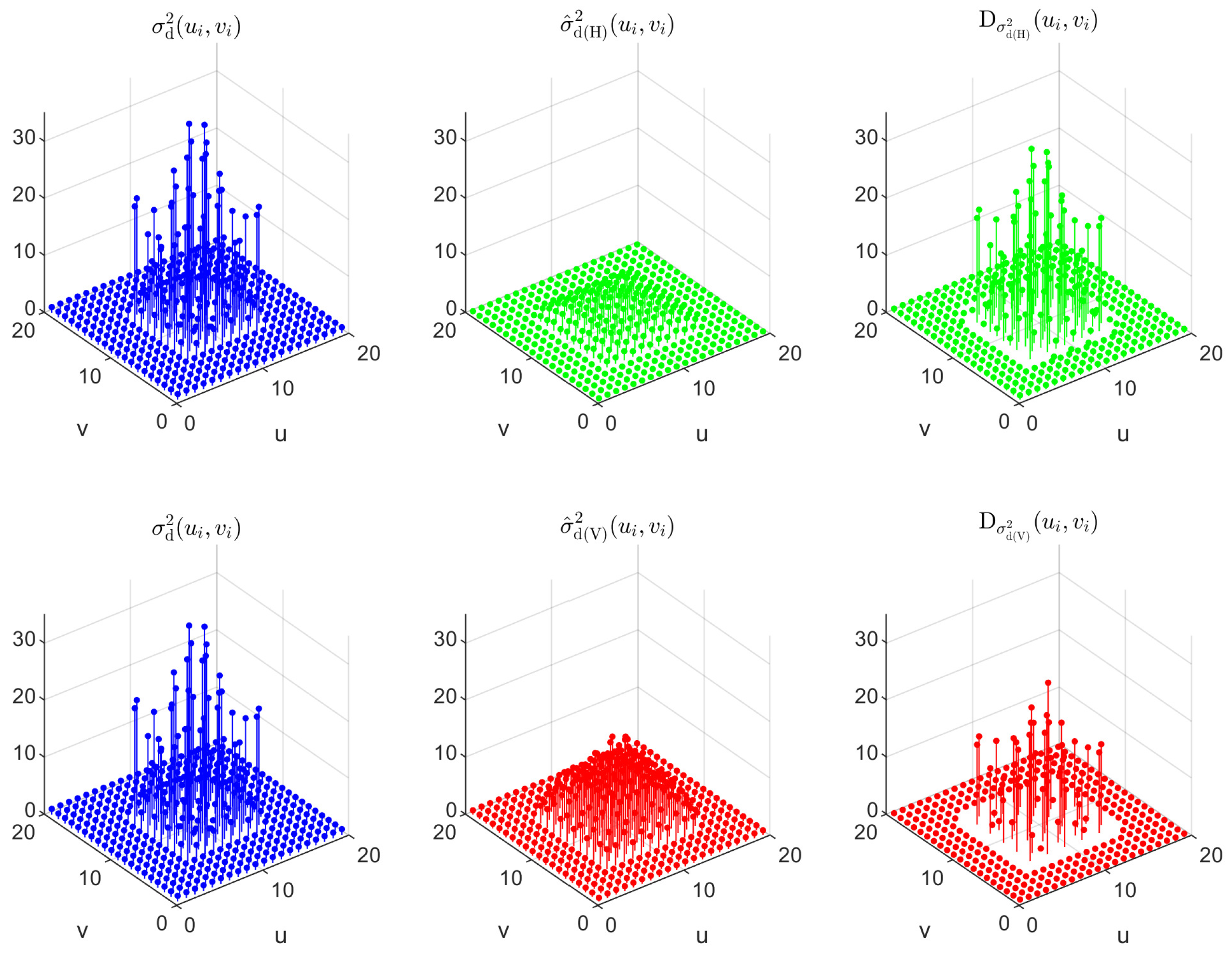
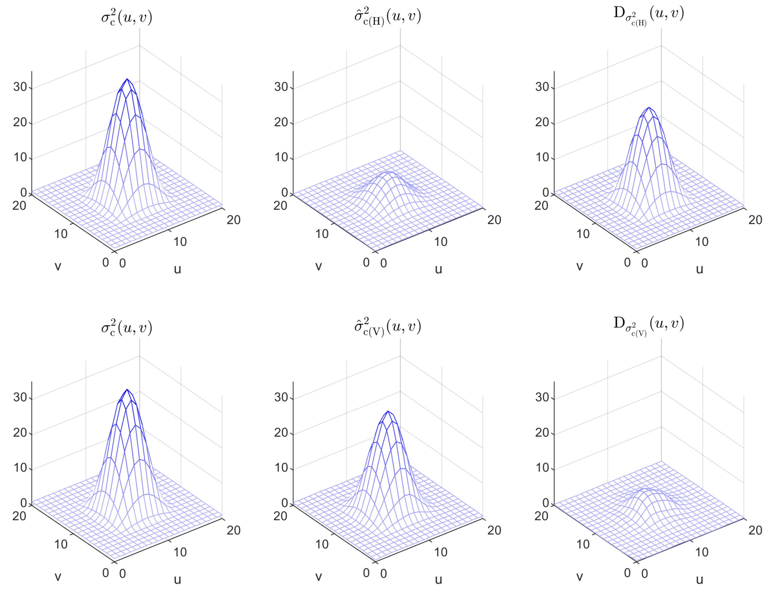
We depict in Figure 1 the final estimators ${\widehat{\sigma }}_{c\left(H\right)}^2(u_i,v_i)$ and ${\widehat{\sigma }}_{c\left(V\right)}^2(u_i,v_i)$ of the variance function ${\sigma }_c^2(u,v)$ of the continuous spatial process $X_c(u,v)$ with their respective pointwise absolute deviations $D_{{\sigma }_{c\left(H\right)}^2}(u_i,v_i)$ and $D_{{\sigma }_{c\left(V\right)}^2}(u_i,v_i)$, and in Figure 2 those of the discrete spatial process $X_d(u_i,v_i)$. Moreover, the graphs of the true variance functions ${\sigma }_c^2(u,v)$ and ${\sigma }_d^2(u_i,v_i)$ are also depicted in Figure 1 and Figure 2 for comparison.

It can be observed from the figures that, for estimating the variance function of a spatial process, the statistic $V_i$ performs much better than $H_i$ in the subregion where both variance functions are spatially varying, while $V_i$ and $H_i$ both yield very accurate estimators in the subregion where the variance functions are constant. Although the estimation accuracy of the variance functions by both statistics shows a decrease in the region where the variance functions are spatially varying, the statistic $V_i$ still performs better than $H_i$. In particular, for the variance function ${\sigma }_d(u_i,v_i)$ that drastically varies in the subregion I and is very hard to accurately estimate in the subregion, $V_i$ still outperforms $H_i$, although the estimation accuracy of both statistics shows an evident decrease in the subregion I. In terms of the overall accuracy measures, we obtained $A{D}_{{\sigma }_{c\left(H\right)}^2}=2.8997$ and $A{D}_{{\sigma }_{c\left(V\right)}^2}=0.6813$ for the continuous spatial process $X_c(u,v)$, and $A{D}_{{\sigma }_{d\left(H\right)}^2}=2.5329$ and $A{D}_{{\sigma }_{d\left(V\right)}^2}=0.4225$ for the discrete spatial process $X_d(u_i,v_i)$, which quantitatively demonstrate that $V_i$ yields more accurate estimators of the variance functions than $H_i$.

The above experimental results seem reasonable according to the different construction orientations of $H_i$ and $V_i$. That is, $H_i$ is constructed as the average of squared residuals in the neighborhood of location i and, as indicated in Ord and Getis [29], is mainly used to identify boundaries of clusters and describing the nature of heteroscedasticity within clusters, while $V_i$ is directly formulated by the sample variance of the observations in the neighborhood of location i for estimating local variance of the underlying spatial process at location i. The results are also consistent with the qualitative conclusion drawn from the theoretical relationship between $H_i$ and $V_i$. That is, $V_i$ is more suitable to estimate the variance function of the spatial process than $H_i$.

3.4. Performance of the $T_{H_i}$-Based and $T_{V_i}$-Based Tests in Detecting Local Spatial Heteroscedasticity

3.4.1. Hypotheses and Indicator for Assessing the Testing Performance

In terms of the statistical hypothesis testing methodology, to detect the local spatial heteroscedasticity of a spatial process amounts to the test for the following null and alternative hypotheses that

$$\begin{array}{c}\hfill \left\{\begin{array}{c}{H}_0^{\left(i\right)}:\mathrm{no}\mathrm{local}\mathrm{heteroscedasticity}\mathrm{exists}\mathrm{at}\mathrm{location}i,\hfill \\ H_1^{\left(i\right)}:\mathrm{local}\mathrm{heteroscedasticity}\mathrm{actually}\mathrm{exists}\mathrm{at}\mathrm{location}i\hfill \end{array}\right.\end{array}$$

at each of the n sampling locations.

As is known in statistics, given a null hypothesis $H_0$ versus the associated alternative hypothesis $H_1$ and a significance level $\alpha$, the rate of rejecting the null hypothesis $H_0$ (i.e., the p-value being less than $\alpha$) in N experiment replications is an estimator of the type I error of the test when the null hypothesis $H_0$ is true, and it measures the power of the test when the alternative hypothesis $H_1$ is true. We then took the rejection rate in N experimental replications under a given significance level as the indicator to assess the performance of the $T_{H_i}$-based and $T_{V_i}$-based tests in detecting the local spatial heteroscedasticity.

Specifically, based on the experimental data generated by the foregoing spatial processes $X_c(u,v)$ and $X_d(u_i,v_i)$, we took both $T_{H_i}$ and $T_{V_i}$ as test statistics and employed their respective bootstrap procedures to derive the p-values at each sampling location. Two commonly used significance levels, $\alpha =0.05$ and 0.10, as well as the corresponding significance levels adjusted by the FDR procedure were taken to determine whether the null hypothesis $H_0^{\left(i\right)}$ at each location can be rejected or not. The experiment was repeated $N=200$ times to compute the rejection rate in each experimental setting. In each experiment replication, $m=1000$ bootstrap samples were drawn from the observations to calculate the p-value of the $T_{H_i}$-based and $T_{V_i}$-based tests, respectively.

3.4.2. Experimental Results with Discussion

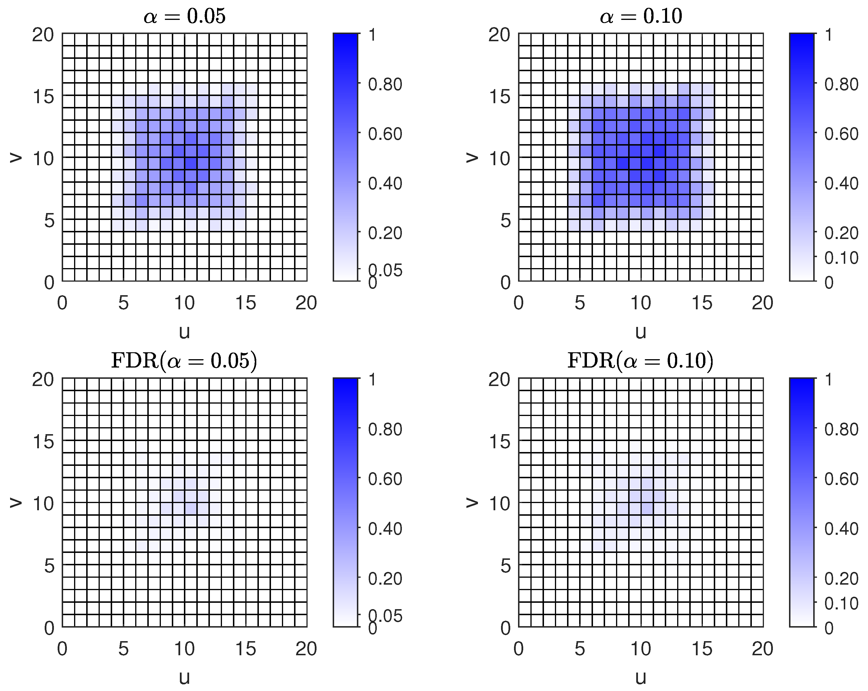
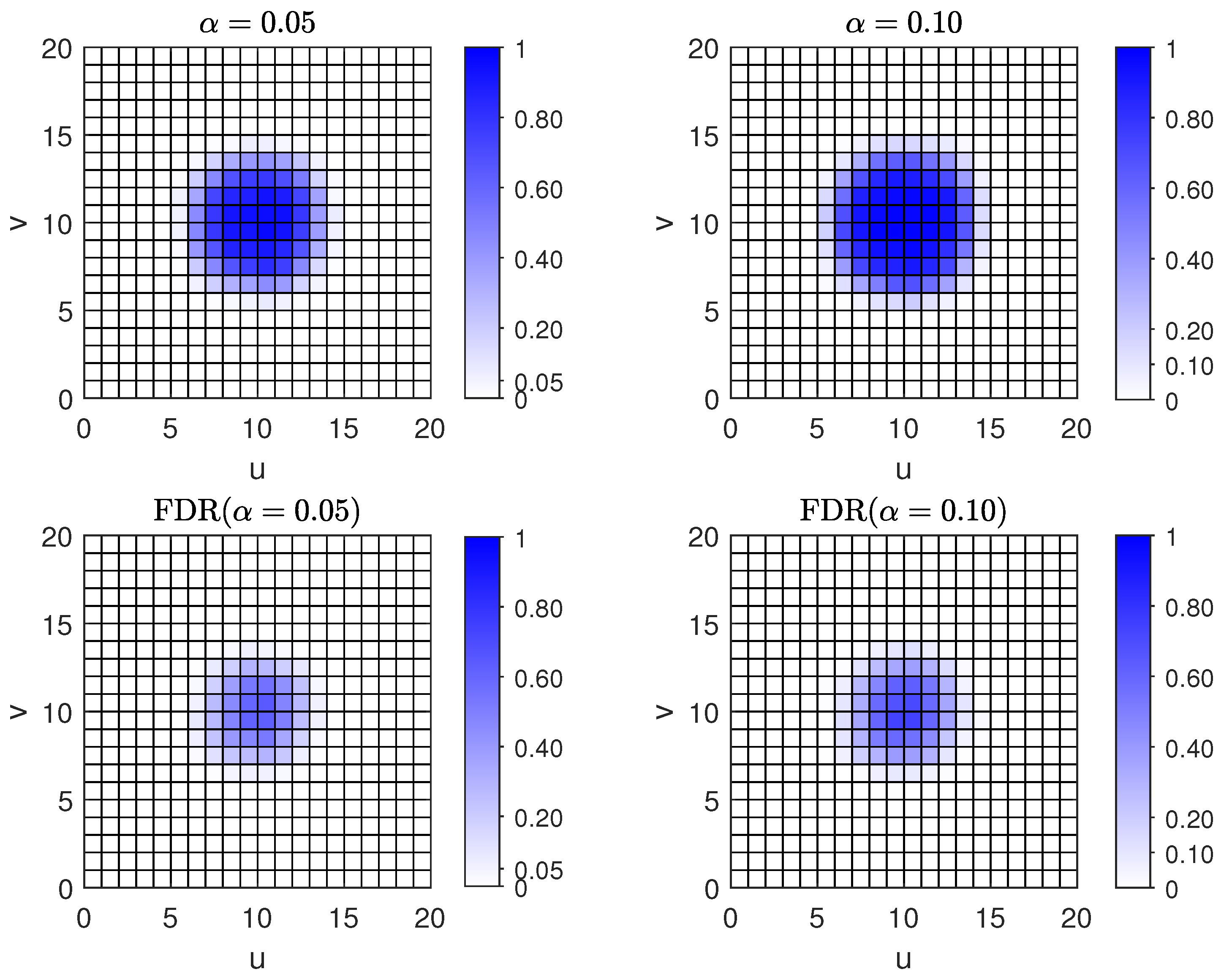
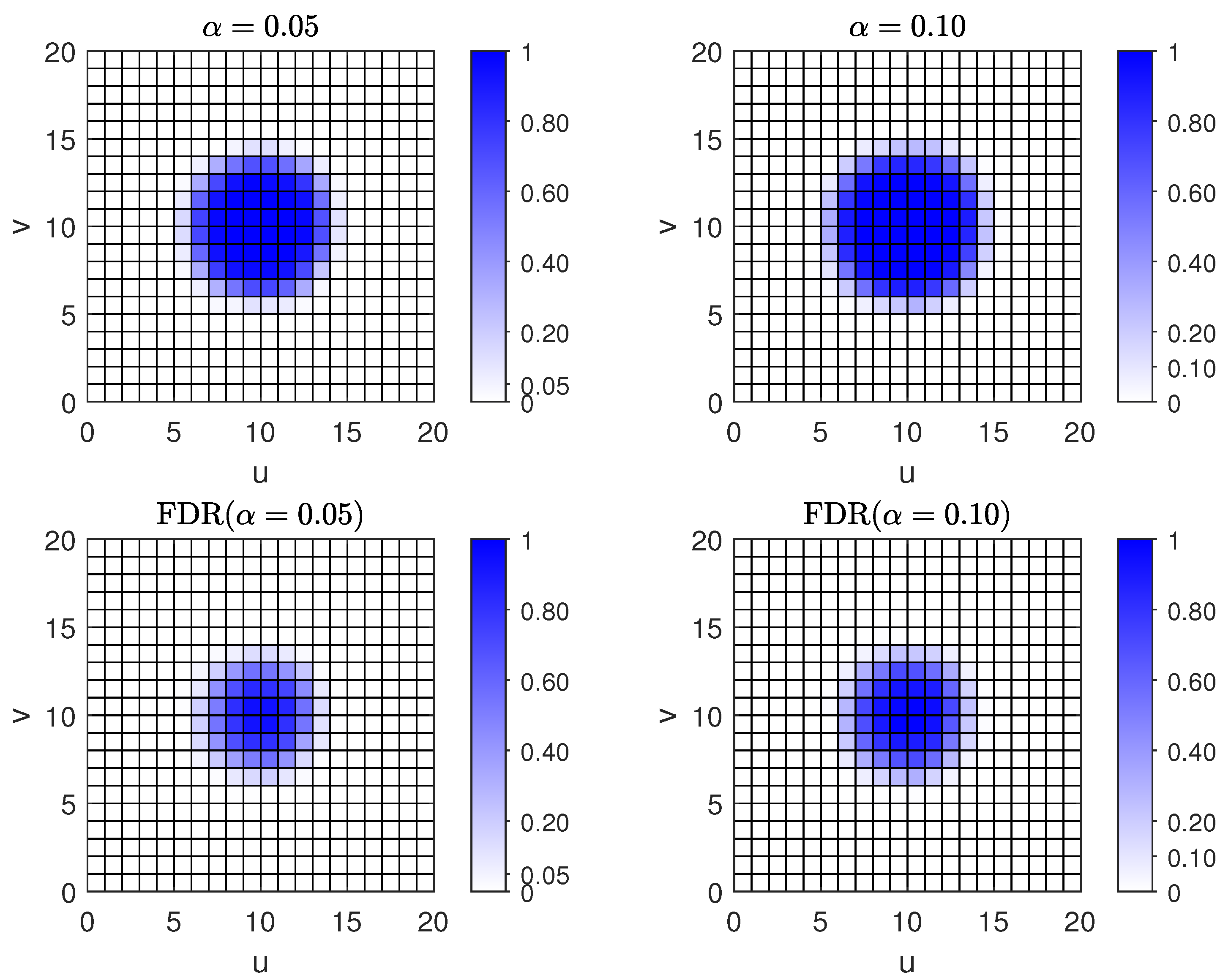
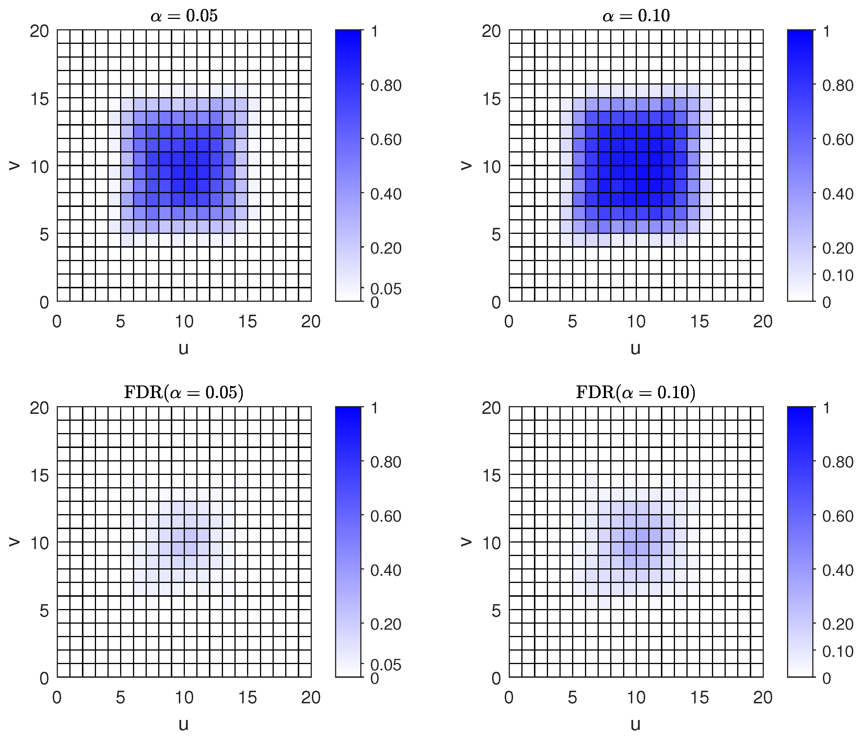
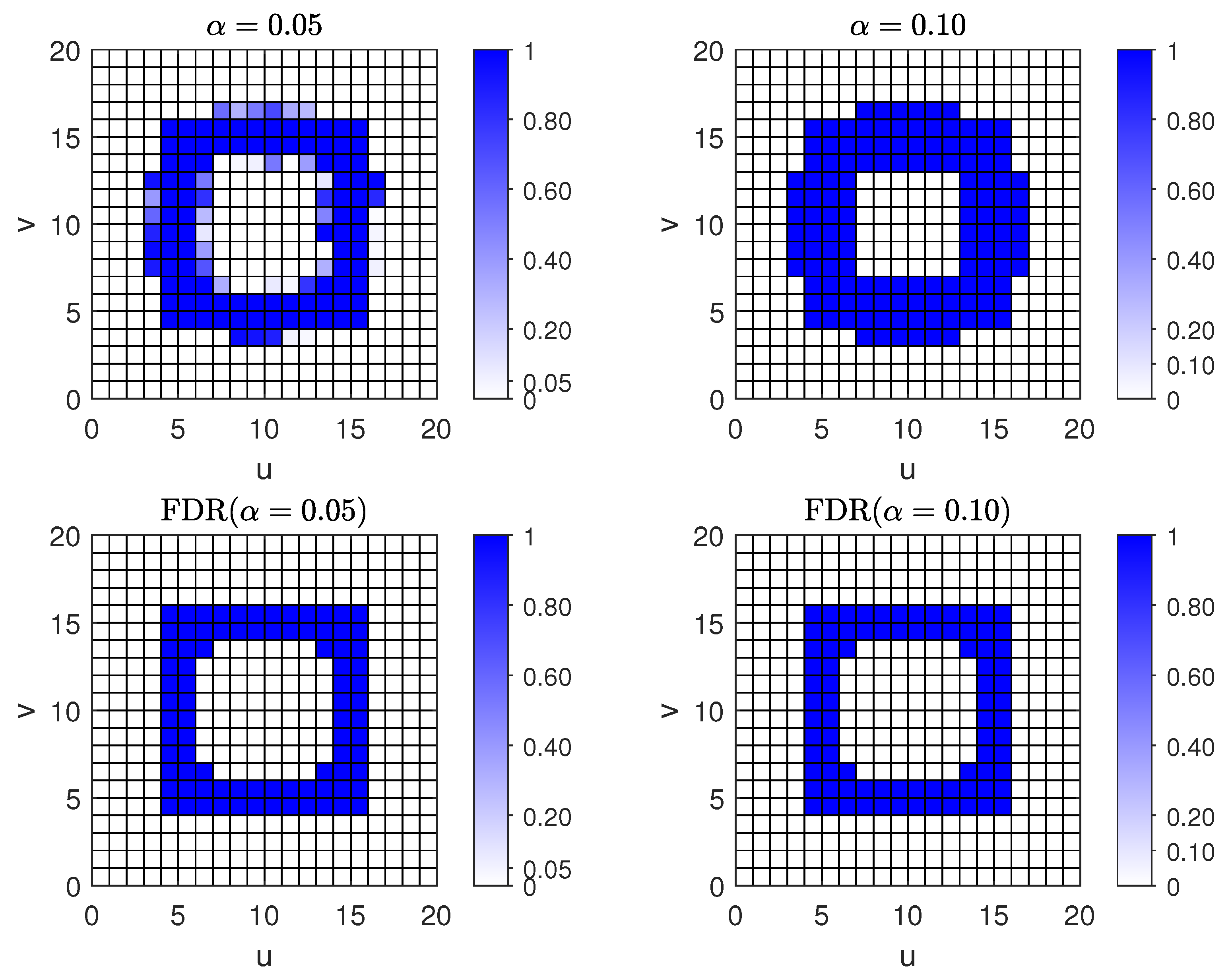
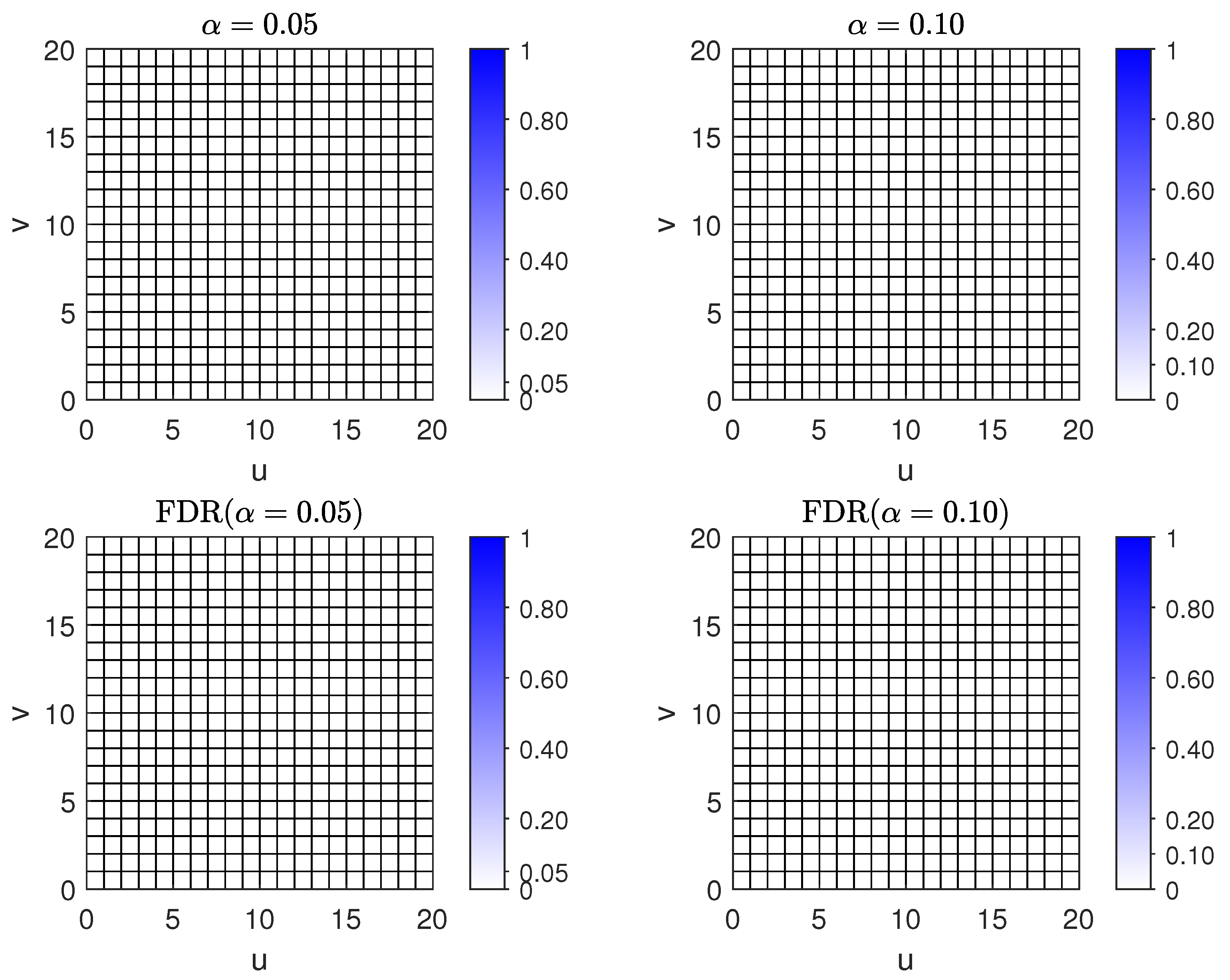
Figure 3 and Figure 4 show the heatmaps of the rejection rates of the $T_{H_i}$-based and $T_{V_i}$-based tests, respectively, for the continuous spatial process $X_c(u,v)$ under the significance levels of $\alpha =0.05$ and 0.10 and those adjusted by FDR in each experiment replication. Figure 5 and Figure 6 illustrate the corresponding heatmaps for the discrete spatial process $X_d(u_i,v_i)$. The overall significance level $\alpha =0.05$ or 0.10 is particularly marked on the colorbar of each subfigure to help evaluate the type I error of each test.

As indicated at the end of Section 3.2.1 and shown from the true surfaces of the variance functions ${\sigma }_c^2(u,v)$ and ${\sigma }_d^2(u_i,v_i)$ in the first column of Figure 1 and Figure 2, both spatial processes are spatially homoscedastic in the surrounding area S and spatially heteroscedastic in the inner area I with the degree of heteroscedasticity increasing from the boundary of I to its center. Therefore, the rejection rate at each location in S reflects the type I error of each test and that in I measures the power of each test.

Focusing on the subregion S in each of the heatmaps in Figure 3, Figure 4, Figure 5 and Figure 6, it is observed that the rejection rates under the various significance levels are consistently less than the corresponding significance levels, indicating that both tests performs well in controlling the type I error.

Regarding the power of the tests, it is observed from Figure 3, Figure 4, Figure 5 and Figure 6 that both $T_{H_i}$-based and $T_{V_i}$-based tests can correctly identify the heteroscedasticity areas of the two spatial processes with a relatively higher rejection rate and an increasing trend from the boundary to the center of the subregion I. In contrast, the $T_{V_i}$-based test is more powerful than the $T_{H_i}$-based test in identifying local spatial heteroscedasticity. Even for the discrete spatial process $X_d(u_i,v_i)$, the $T_{V_i}$-based test is still evidently more powerful than the $T_{H_i}$-based test, although both tests show decreasing power in detecting the local heteroscedasticity. As specific evidence, under the significance level $\alpha =0.05$, the top five maximal values of the rejection rate of the $T_{V_i}$-based test are 1.00, 0.995, 0.990, 0.985, and 0.975 with the numbers of the corresponding cells being 11, 2, 1, 3, and 3, respectively, for the continuous spatial process, and they are 0.845, 0.835, 0.830, 0.825, and 0.820 with the numbers of the corresponding cells being 1, 1, 1, 2, and 2, respectively, for the discrete spatial process. The top five maximal values of the rejection rate of the $T_{H_i}$-based test are 0.965, 0.950, 0.945, 0.940, and 0.925 with the numbers of the corresponding cells being 1, 1, 1, 1, and 2, respectively, for the continuous spatial process, and they are 0.700, 0.615, 0.595, 0.585, and 0.575 with the numbers of the corresponding cells being 1, 1, 1, 1, and 2, respectively, for the discrete spatial process.

These results are reasonable because, as demonstrated in the simulation study performed in Section 3.3, $V_i$ can yield a more accurate estimator than $H_i$, leading to the more powerful $T_{V_i}$-based test in detecting the local spatial heteroscedasticity. Interestingly, however, the $T_{H_i}$-based test is still of relatively high power in detecting the local spatial heteroscedasticity especially for the continuous spatial process, even if $H_i$ is sensitive to local structural changes rather than the variance magnitude itself drawn from the theoretical relationship between $H_i$ and $V_i$ in Section 2.3.

In regard to the FDR procedure for dealing with the involved multiple testing issue, it can be observed from the corresponding subfigures in Figure 3, Figure 4, Figure 5 and Figure 6 that this procedure seems very conservative in each of the experiment settings, because many locations where local spatial heteroscedasticity actually exists are neglected under the adjusted significance levels, leading to a much lower rejection rate in the inner area I. However, compared with the Bonferroni procedure where the adjusted significance levels are respectively ${\alpha }_J=0.05/400=1.25\times {10}^{-4}$ and ${\alpha }_J=0.10/400=2.5\times {10}^{-4}$ in our cases, the FDR procedure is slightly more powerful. In fact, we used the Bonferroni procedure to deal with the multiple testing issue in each of the experiment settings and the resulting rejection rates for both spatial processes are all very close to zero over the whole spatial region, indicating that the Bonferroni procedure is more conservative than the FDR procedure.

3.5. Performance of the $T_{H_i}$-Based and $T_{V_i}$-Based Tests in Identifying Boundaries of Spatial Homogeneous Clusters

3.5.1. Hypotheses and Indicator for Assessing the Identification Performance

In this subsection, we will evaluate the performance of the $T_{H_i}$-based and $T_{V_i}$-based tests in identifying the boundaries of spatial homogeneous clusters. The boundaries of spatial homogeneous clusters or the transitional areas from one homogeneous cluster to another imply that the structure in the value of a spatial process changes. Therefore, to identify whether location i is on the boundaries of spatial homogeneous clusters amounts to the test for the following null and alternative hypotheses that

$$\begin{array}{c}\hfill \left\{\begin{array}{c}{H}_0^{\left(i\right)}:\mathrm{there}\mathrm{is}\mathrm{no}\mathrm{structural}\mathrm{change}\mathrm{in}\mathrm{value}\mathrm{at}\mathrm{location}i,\hfill \\ H_1^{\left(i\right)}:\mathrm{there}\mathrm{is}\mathrm{structural}\mathrm{change}\mathrm{in}\mathrm{value}\mathrm{at}\mathrm{location}i\hfill \end{array}\right.\end{array}$$

at each of the n sampling locations.

Both $T_{H_i}$-based and $T_{V_i}$-based tests were used to test the above hypotheses at each of the sampling locations and the rate of rejecting the null hypothesis in N experimental replications was once again taken as the indicator for assessing their performance in identifying the boundaries of spatial homogeneous clusters.

Specifically, based on the experimental data generated by the spatial process described in Section 3.2.2, the respective bootstrap procedures of the test statistics $T_{H_i}$ and $T_{V_i}$ were employed to derive p-values of the tests, in which $m=1000$ bootstrap samples were drawn from the set of observations. The experiment was also repeated $N=200$ times to compute the rejection rates under the significance levels $\alpha =0.05$ and 0.10 at all of the sampling locations and the FDR procedure was used to deal with the involved multiple testing issue.

3.5.2. Experimental Results with Discussion

Figure 7 depicts the heatmaps of the rejection rates of the $T_{H_i}$-based test under the significance levels $\alpha =0.05$ and 0.10 and their respective levels adjusted by the FDR procedure in the $N=200$ experiment replications. Figure 8 shows the corresponding heatmaps of the $T_{V_i}$-based test.

Compared with the underlying spatial process described in Section 3.2.2 for generating the experimental data, we can observe from Figure 7 that the $T_{H_i}$-based test is very powerful and of a valid type I error in identifying the boundary of the two homogeneous clusters with, on the one hand, almost all the rejection rates at the boundary cells being equal to 1, although a few of the cells near the boundary are falsely identified to be on the boundary under both the significance levels; on the other hand, the rejection rates at the cells that are relatively far from the boundary are consistently less than their respective significance levels. In contrast, we can see from Figure 8 that the $T_{V_i}$-based test is totally noneffective in identifying the boundaries of spatial homogeneous clusters, because of its nearly zero rejection rates on the whole region. Although the theoretical relationship between $H_i$ and $V_i$ shown in Section 2.3 implies that $H_i$ is sensitive to local structure changes of a spatial process and $V_i$ qualifies to be an estimator of the local variance of a spatial process, such a substantial difference in the performance of the $T_{H_i}$-based and $T_{V_i}$-based tests in identifying the boundaries of homogeneous spatial clusters seems somewhat unexpected. This finding further demonstrates the necessity of the simulation study.

From the two subfigures in the second row of Figure 7, we know that the FDR procedure performs especially well in this case, in view of the fact that almost all the cells that are falsely identified as boundary cells under the overall significance levels have been retrieved to be non-boundary cells under the significance levels adjusted by the FDR procedure. Combining this finding with that observed in Section 3.4.2, we may conclude that the performance of the FDR procedure depends upon the sensitivity of the related test statistic to the target alternative hypothesis.

3.6. Findings from the Simulation Study

Based on the simulation study conducted in this section, we obtain the following findings, which provide useful guidance for the $H_i$ and $V_i$ statistics and their associated tests to be used in practice from different application orientations.

• Both $H_i$ and $V_i$ are qualified to be an estimator of the variance function of a spatial process, while $V_i$ yields a more accurate estimator than $H_i$.
• Both $T_{H_i}$-based and $T_{V_i}$-based tests are of a valid type I error and reasonably high power in detecting the local heteroscedasticity of a spatial process, while the $T_{V_i}$-based test is more powerful than the $T_{H_i}$-based test.
• The $T_{H_i}$-based test is especially powerful in identifying the boundaries of spatial homogeneous clusters, but the $T_{V_i}$-based test is totally noneffective.

4. Applications of the ${\mathit{H}}_{\mathit{i}}$ and ${\mathit{V}}_{\mathit{i}}$ Statistics with Their Associated Tests

Based on the findings in the simulation study, two real-life spatial datasets were analyzed by the $H_i$ and $V_i$ statistics and the associated $T_{H_i}$-based and $T_{V_i}$-based tests to demonstrate their potential applications.

4.1. Local Spatial Heteroscedasticity Detection of Annual Precipitation Amounts

4.1.1. Introduction to the Dataset and Formulation of the Spatial Weights Matrix

The dataset consists of the annual precipitation amounts (mm) collected at the 573 meteorological stations over the mainland of China in 2005 with the longitude and latitude of each meteorological station attached. Of interest is to detect local spatial heteroscedasticity, identify possible boundaries of precipitation clusters, and uncover the nature of heteroscedasticity within the clusters of precipitation amounts.

Since the meteorological stations distribute irregularly over the space, we used a fixed distance threshold to specify the adjacency relationship between a reference station and its nearby stations and further formulated the spatial weights matrix. Specifically, the Euclidean distance was used to determine the neighborhood of a reference station. For simplicity, we transformed the longitude and latitude of each station into the Cartesian coordinates by the Gauss–Krüger projection under the Xi’an 80 geodetic coordinate system of China with the origin being at (${108}^{°}{55}^{\prime }$ E, ${34}^{°}{32}^{\prime }$ N). Let $d_{ij}$ be the Euclidean distance between stations i and j. The spatial weights matrix $\mathit{W}={\left(w_{ij}\right)}_{n\times n}$ was specified in what follows. Given a distance threshold d and a reference meteorological station i, the spatial weights at station i were specified as

$$\begin{array}{c}\hfill w_{ij}=\left\{\begin{array}{cc}1,\hfill & \mathrm{if}{d}_{ij}\le d;\hfill \\ 0,\hfill & \mathrm{if}{d}_{ij}>d,\hfill \end{array}\right.j=1,2,\cdots ,n,\end{array}$$

(13)

where $n=573$. This kind of spatial weights matrix automatically satisfies $w_{ii}=1$ for $i=1,2,\cdots ,n$. In order to assess the robustness of the testing results with respect to the spatial weights matrix, we considered three different spatial weights matrices generated by assigning the distance threshold d to be $d_1=250\mathrm{km}$, $d_2=300\mathrm{km}$, and $d_3=350\mathrm{km}$, respectively. The resulting three spatial weights matrices are henceforth denoted by ${\mathit{W}}_1$, ${\mathit{W}}_2$, and ${\mathit{W}}_3$, respectively, for ease of presentation.

Note. It needs to be pointed that the Gauss–Krüger projection is a zoned projection originally designed to minimize distortion within a small area. Here, the entire area spanning over 60 degrees of longitude was projected onto a single Gauss–Krüger projection plane, which could lead to extremely severe distance and area distortions at the eastern and western edges, and consequently the inconsistent interpretations between the reality and the adjacency relationships derived by the assigned distance thresholds. However, our purpose is to generate different spatial weights matrices for assessing the robustness of the testing results to the variation in the spatial weights matrix and the assigned three distance thresholds can indeed generate quite different spatial weights matrices. For convenience, we used a single Gauss–Krüger projection to achieve the task.

4.1.2. Testing Results with Discussion

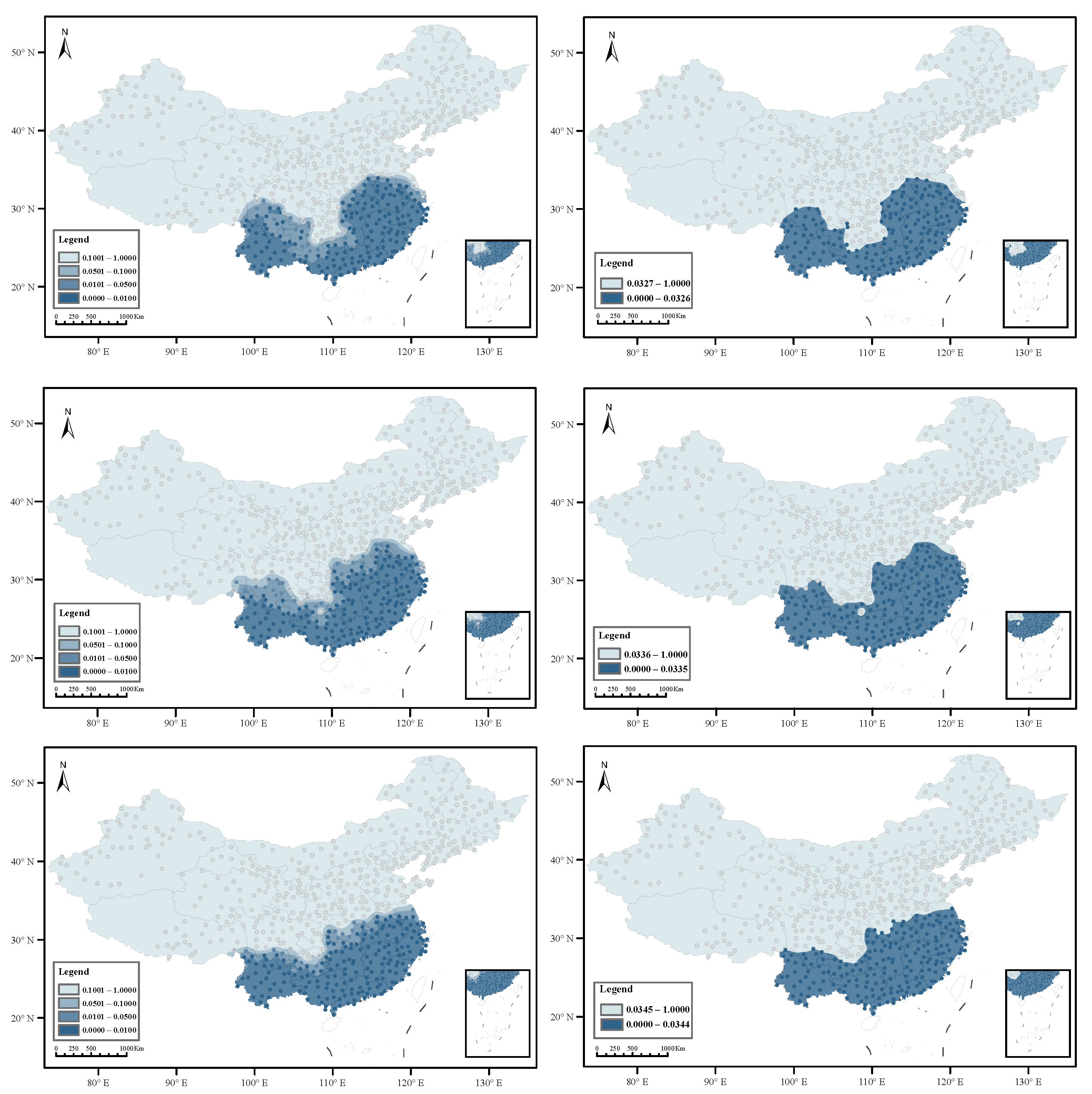
Both $T_{H_i}$-based and $T_{V_i}$-based tests with their respective bootstrap procedures were employed to perform the analysis, in which $m=1000$ bootstrap samples were drawn from the observed annual precipitation amounts to derive p-values of both tests at each meteorological station. Furthermore, the FDR procedure was used to deal with the multiple testing issue. Figure 9 shows the heatmaps of the p-values of the $T_{H_i}$-based test under the three spatial weights matrices ${\mathit{W}}_1$, ${\mathit{W}}_2$, and ${\mathit{W}}_3$. The heatmaps of the p-values under the three spatial weights matrices (left column in Figure 9) are depicted as four-color graphs with the four colored areas separated by the commonly used significance levels of $\alpha =0.01,0.05,$ and 0.10 in order to clearly show the transitional areas from each significance level to another. The corresponding heatmaps under the three spatial weights matrices (right column of Figure 9) are depicted as bi-color graphs with the two colored areas in each heatmap separated by the adjusted significance level ${\alpha }_J$ under the overall significance level of $\alpha =0.10$ to show the effectiveness of the FDR procedure. In regard to the results of the $T_{V_i}$-based test, however, the p-values under the three spatial weights matrices are all sufficiently large over the entire region, indicating insignificant testing results over the region. We therefore omitted the heatmaps to save space.

First, in view of the findings in the simulation study that the $T_{V_i}$-based test is powerful in detecting spatial heteroscedasticity, but is noneffective in identifying boundaries of spatial homogeneous clusters, the large p-values of the $T_{V_i}$-based test over the whole region imply that the annual precipitation amounts are homoscedastic over the mainland of China. That is to say, the annual precipitation amounts are homogeneous in variance. However, based on the finding in the simulation study that the $T_{H_i}$-based test is especially powerful in identifying the boundaries of spatial homogeneous clusters, we know from Figure 9 that the annual precipitation amounts shape into two clusters with a clear boundary partitioning the whole region into northern and southern parts under all of the significance levels $\alpha =0.01$, 0.05, and 0.10. Furthermore, according to the theoretical finding in Section 2 that $H_i$ is sensitive to local structure changes rather than the variance magnitude itself, we may conclude that the annual precipitation amounts form a homogeneous cluster in value in the extensive northern area, while they show a heterogeneous cluster in value in the southern area. Given the conclusion drawn from the $T_{V_i}$-based test that the annual precipitation amounts are homoscedastic over the space, we may affirm that the spatial heterogeneity of the annual precipitation amounts in the heterogeneous cluster is mainly due to different precipitation amounts at the meteorological stations over the southern part. This is in accord with the climate characteristics that precipitation is plentiful in the southern area of China and the amounts vary markedly from place to place. Moreover, the heatmaps of the p-values of the $T_{H_i}$-based test show a very similar spatial pattern for the three different spatial weights matrices, indicating that the test is robust to the spatial weights matrix for this dataset. Finally, from the above analysis, we may recognize that the combination of the result from the $T_{H_i}$-based test with that from the $T_{V_i}$-based test can yield a deeper understanding about the nature of heterogeneity within clusters.

From the heatmaps in the right column of Figure 9, we observed that the FDR procedure is of high effectiveness in dealing with the multiple testing issue involved in the $T_{H_i}$-based test. The area where the heterogeneous cluster locates under the overall significance level of $\alpha =0.10$ shows a slight shrinkage under all of the adjusted significance levels of ${\alpha }_J$ = 0.0326, 0.00335, and 0.0344. Furthermore, compared with the significance level adjusted by the Bonferroni procedure, which is ${\alpha }_J=0.10/573=1.745\times {10}^{-4}$ for the three spatial weights matrices, the significance levels adjusted by the FDR procedure are much larger, indicating that the FDR procedure is much more powerful than the Bonferroni procedure for this dataset.

4.2. Geographically Weighted Regression (GWR) Modeling for the Dublin Voter Turnout Data

4.2.1. Introduction to the Dataset and Formulation of the Spatial Weights Matrix

The Dublin voter turnout dataset, which is publicly available in the R package linked to [43], includes the observations of nine variables in 322 Electoral Divisions (EDs) of Greater Dublin in the Irish 2004 Dáil elections. The Cartesian coordinates $(u,v)$ of each ED are also attached to the data. The nine variables are as follows.

• PVE: percentage of the population who voted in the election;
• OYM: percentage of one year migrants;
• LAR: percentage of local authority renters;
• SCO: percentage of the population in high social class;
• UEP: percentage of the unemployed population;
• LOE: percentage of the population without any formal education;
• AGY: percentage of the population aged from 18 to 24 years;
• AGM: percentage of the population aged from 25 to 44 years;
• AGO: percentage of the population aged from 45 to 64 years.

We formulated the spatial weights matrix $\mathit{W}={\left(w_{ij}\right)}_{n\times n}$ via the queen scheme, i.e.,

$$\begin{array}{c}\hfill w_{ij}=\left\{\begin{array}{cc}1,\hfill & \mathrm{if}\mathrm{EDs}i\mathrm{and}j\mathrm{share}\mathrm{a}\mathrm{common}\mathrm{boundary},\hfill \\ 0,\hfill & \mathrm{otherwise},\hfill \end{array}\right.\end{array}$$

(14)

where $1\le i\ne j\le n$ with $n=322$. In particular, we set $w_{ii}=1$ for $i=1,2,\cdots ,n$.

4.2.2. Semi-Parametric GWR Model for the Dataset

For this dataset, it is of interest to explore the spatial heterogeneity of the effect of the eight social structure variables on the percentage of the population who voted in the election (PVE). As a powerful tool for exploring spatial heterogeneity in regression relationships, GWR models [32] are competent to achieve the task. Lu et al. [44] established the GWR model between PVE and the social structure variables and employed the Monte Carlo test to identify constant coefficients. Consequently, they obtained the following semi-parametric GWR model:

$$\begin{array}{cc}\hfill {\mathrm{PVE}}_i& ={\beta }_0+{\beta }_1{\mathrm{OYM}}_i+{\beta }_2{\mathrm{LAR}}_i+{\beta }_3{\mathrm{LOE}}_i+{\beta }_4{\mathrm{AGM}}_i+{\beta }_5{\mathrm{AGO}}_i+{\beta }_6(u_i,v_i){\mathrm{SCO}}_i\hfill \\ \hfill & +{\beta }_7(u_i,v_i){\mathrm{UEP}}_i+{\beta }_8(u_i,v_i){\mathrm{AGY}}_i+{\epsilon }_i,i=1,2,\cdots ,n.\hfill \end{array}$$

(15)

Lu et al. [44] further used the two-step estimation (TSE) method [45] to calibrate the above model, where the model errors ${\epsilon }_i$s were assumed to be homoscedastic. As is well known in regression analysis, however, violation of this assumption may lead to inefficient estimation of the model and some diagnostic tool and remedial measures must be exercised for the heteroscedasticity of model errors. When the model errors are really heteroscedastic, a common way to deal with heteroscedasticity in model errors is to employ the generalized least-squares procedure for model calibration, in which an efficient estimator of the variance function of the model error term is crucial. As demonstrated in the foregoing simulation study, both $T_{H_i}$-based and $T_{V_i}$-based tests can provide a diagnostic tool for the spatial heteroscedasticity of model errors and both $H_i$ and $V_i$ statistics are eligible to be an estimator of the variance function of model error term.

Since the main focus here is to demonstrate the applications of the $H_i$ and $V_i$ statistics with their associated tests, we therefore start from the semi-parametric GWR model in Equation (15) to detect the spatial heteroscedasticity of the model errors. If the model errors are spatially heteroscedastic, the generalized least-squares procedure is employed to re-calibrate the model based on the TSE procedure of semi-parametric GWR models. For the coherence and readability of this paper, the TSE procedure with the related issues is postponed to Appendix A.

4.2.3. Detection of Spatial Heteroscedasticity in the Model Errors

We first calibrated the semi-parametric GWR model in Equation (15) by the TSE procedure and obtained the residuals ${\widehat{\epsilon }}_1,{\widehat{\epsilon }}_2,\cdots ,{\widehat{\epsilon }}_n$ at the optimal bandwidth size $h_0$. As shown in Appendix A, the bi-square kernel with an adaptive bandwidth was used to generate the weights in the TSE procedure and the optimal bandwidth size $h_0$ was selected by the AICc criterion. The resulting optimal bandwidth size is $h_0=28$ EDs. We based the residuals to formulate the test statistics

$$\begin{array}{c}\hfill T_{H_i}={\displaystyle \frac{{\displaystyle \sum _{j=1}^n}{w}_{ij}{\left({\widehat{\epsilon }}_j-{\overline{\widehat{\epsilon }}}_j\right)}^2}{h_1{\displaystyle \sum _{j=1}^n}{w}_{ij}}}\mathrm{and}{T}_{V_i}={\displaystyle \frac{{\displaystyle \sum _{j=1}^n}{w}_{ij}{\left({\widehat{\epsilon }}_j-{\overline{\widehat{\epsilon }}}_i\right)}^2}{\frac{1}{n}{\displaystyle \sum _{j=1}^n}{\left({\widehat{\epsilon }}_j-\overline{\widehat{\epsilon }}\right)}^2{\displaystyle \sum _{j=1}^n}{w}_{ij}}}\end{array}$$

to detect the local spatial heteroscedasticity in the model errors, where $w_{ij}$ ($1\le i,j\le n$) are the elements of the spatial weights matrix $\mathit{W}$ specified by Equation (14), $h_1={\displaystyle \sum _{j=1}^n}{\left({\widehat{\epsilon }}_j-{\overline{\widehat{\epsilon }}}_j\right)}^2/n$ with ${\overline{\widehat{\epsilon }}}_j={\displaystyle \sum _{k=1}^n}{w}_{jk}{\widehat{\epsilon }}_k/{\displaystyle \sum _{k=1}^n}{w}_{jk}$, and $\overline{\widehat{\epsilon }}={\displaystyle \sum _{j=1}^n}{\widehat{\epsilon }}_j/n$. We then adopted their respective bootstrap procedures to compute the p-values of the $T_{H_i}$-based and $T_{V_i}$-based tests at each ED, in which $m=1000$ bootstrap samples were drawn from the residuals ${\widehat{\epsilon }}_1,{\widehat{\epsilon }}_2,\cdots ,{\widehat{\epsilon }}_n$ to compute the p-values.

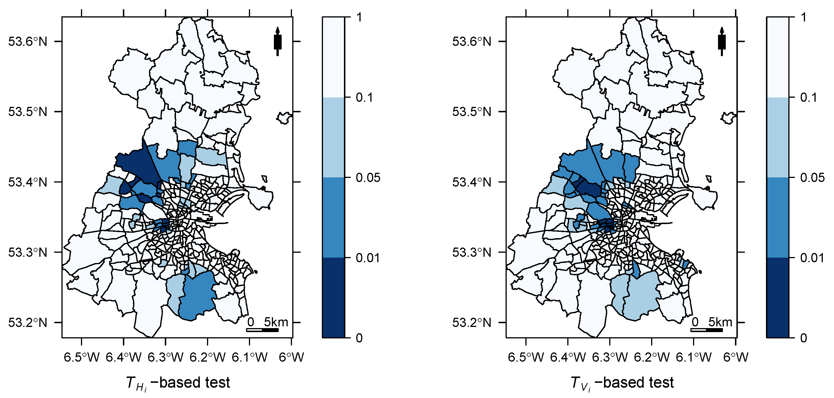
Figure 10 depicts the heatmaps of the p-values for the two tests. Both heatmaps show that local spatial heteroscedasticity exists in the model errors even under the significance level of $\alpha =0.01$. In detail, the EDs where the model errors are heteroscedastic are mainly located in the middle and south areas. The number of the EDs with p-values being less than $0.05$ is 33 for the $T_{V_i}$-based test and is 26 for the $T_{H_i}$-based test, indicating that the $T_{V_i}$-based test is more powerful in detecting the local spatial heteroscedasticity, which is consistent with the finding in the simulation study.

4.2.4. Generalized Least-Squares Estimation (GLSE) of the Model

As aforementioned, the GLSE procedure is commonly adopted to improve the estimation efficiency of a heteroscedastic regression model, where an estimator of the variance function of model errors is needed to weight the data and consequently make the model errors homoscedastic. As shown in the simulation study in Section 3.3, the LOVA statistic $V_i$ yields a more accurate estimator of the variance function of a spatial process than the LOSH statistic $H_i$. We therefore took the residuals ${\widehat{\epsilon }}_1,{\widehat{\epsilon }}_2,\cdots ,{\widehat{\epsilon }}_n$ from the TSE procedure as observations of the model error term to formulate the LOVA statistic, which shows

$$\begin{array}{c}\hfill V_i={\displaystyle \frac{{\displaystyle \sum _{j=1}^n}{w}_{ij}{\left({\widehat{\epsilon }}_j-{\overline{\widehat{\epsilon }}}_i\right)}^2}{{\displaystyle \sum _{j=1}^n}{w}_{ij}}},i=1,2,\cdots ,n\end{array}$$

(16)

at the EDs. The observations of both response variable and explanatory variables were weighted by the reciprocals of the square root of $V_i$s, on which the model in Equation (15) was re-calibrated by the TSE procedure. Specifically, let

$$\begin{array}{c}\hfill \tilde{\mathit{y}}={\mathit{V}}^{-1/2}\mathit{y},{\tilde{\mathit{X}}}_c={\mathit{V}}^{-1/2}{\mathit{X}}_c,{\tilde{\mathit{X}}}_v={\mathit{V}}^{-1/2}{\mathit{X}}_v,\end{array}$$

where

$$\begin{array}{c}\hfill {\mathit{V}}^{-1/2}=\mathrm{Diag}\left({\displaystyle \frac{1}{\sqrt{V_1}}},{\displaystyle \frac{1}{\sqrt{V_2}}},\cdots ,{\displaystyle \frac{1}{\sqrt{V_n}}}\right),\end{array}$$

and $\mathit{y}$, ${\mathit{X}}_c$, and ${\mathit{X}}_v$, as shown in Appendix A in Equation (A2), are the observations vector of the response variable PVE, the observations matrix of the explanatory variables with constant coefficients, and that of the explanatory variables with spatially varying coefficients, respectively. Here, all the elements in the first column of ${\mathit{X}}_c$ are 1 due to the constant intercept in the model in Equation (15). Replacing $\mathit{y}$, ${\mathit{X}}_c$, and ${\mathit{X}}_v$ with the transformed data $\tilde{\mathit{y}}$, ${\tilde{\mathit{X}}}_c$, and ${\tilde{\mathit{X}}}_v$, respectively, and setting the value of the bandwidth h to be its optimal size $h_0$ to conduct the TSE procedure in the appendix, we finally obtained the GLSE estimators of the constant coefficients ${\beta }_0,{\beta }_1,\cdots ,{\beta }_5$ and those of the spatially varying coefficients ${\beta }_6(u_i,v_i),{\beta }_7(u_i,v_i),{\beta }_8(u_i,v_i)$ at each ED.

Furthermore, we computed the goodness-of-fit statistics $R^2$ and AICc at the optimal bandwidth size $h_0$ for both TSE and GLSE to evaluate the model fit performance of the two estimation methods.

4.2.5. Estimation Results with Comparison to the TSE Results

Table 1. Values of the estimated constant coefficients and the goodness-of-fit statistics for the two estimation methods.

Method	Constant Coefficient						Goodness-of-Fit Statistic
	${\mathit{\beta }}_{\mathbf{0}}$	${\mathit{\beta }}_{\mathbf{1}}$	${\mathit{\beta }}_{\mathbf{2}}$	${\mathit{\beta }}_{\mathbf{3}}$	${\mathit{\beta }}_{\mathbf{4}}$	${\mathit{\beta }}_{\mathbf{5}}$	${\mathit{R}}^{\mathbf{2}}$	AICc
GLSE	92.4752	−0.0840	−0.1116	0.3836	−0.6275	−0.2667	0.7993	3.8306
TSE	90.5472	−0.0804	−0.1071	0.2482	−0.5910	−0.3298	0.7582	6.0594
Variable	Intercept	OYM	LAR	LOE	AGM	AGO	—	—

reports the estimated values of the constant coefficients in the model in Equation (15) and the values of the goodness-of-fit statistics $R^2$ and AICc resulting from the GLSE method. For comparison, the estimated values of the constant coefficients and the values of $R^2$ and AICc obtained from the TSE method are also listed in the table. Moreover, for ease of the interpretation of the results, the explanatory variables related to the constant coefficients are also attached in the last row of the table where the variable corresponding to the constant intercept ${\beta }_0$ is labeled as “Intercept".

First, we know from the table that, as expected, the GLSE method yields a better model fit in terms of $R^2$ and AICc in view of the large value in $R^2$ and smaller value in AICc for the GLSE method. The corresponding estimated values of the constant coefficients by the two methods all share the same sign. This leads to a consistent qualitative interpretation for the effect of the corresponding explanatory variables on the response variable PVE. That is, LOE positively influences PVE, while OYM, LAR, AGM, and AGO negatively influence PVE. Since the GLSE method generally yields more accurate estimators of the coefficients, more precise quantitative analysis of the effect of these explanatory variables on PVE can be acquired using the specific estimated values yielded by the GLSE method.

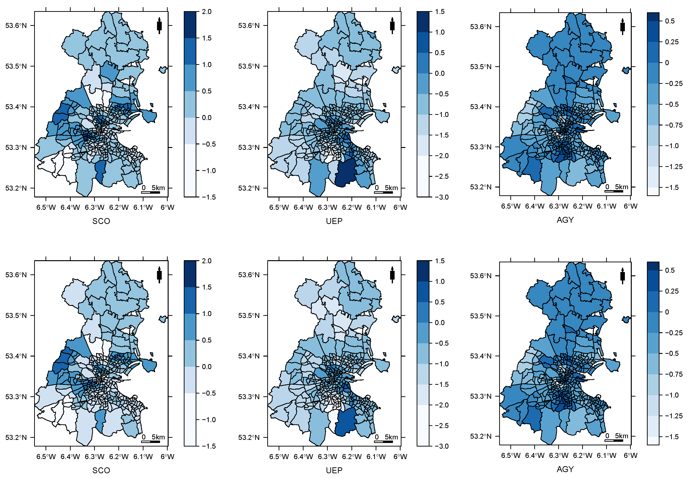
Figure 11 depicts the heatmaps of the estimators of the spatially varying coefficients in the model in Equation (15) obtained by both the GLSE and TSE methods, where the spatially varying coefficients are labeled by the names of their respective explanatory variables.

Comparing the heatmaps of the spatially varying coefficient estimators yielded by the GLSE method with those of the estimators obtained by the TSE method, we can observe that some local differences do exist, although the basic spatial pattern of each spatially varying coefficient estimator is correspondingly similar. Generally speaking, all of the explanatory variables SCO, UEP, and AGY show either a positive or negative effect on PVE over the EDs. Specifically, SCO shows a positive effect in most EDs and an extremely negative effect in several EDs located in the center and southwest area; UEP has, in general, a negative effect over the EDs except for several EDs in the south and center area; AGY shows a complex pattern of effect on PVE: except for the EDs showing a weak negative effect in the north area, the EDs with positive effect and those with negative effect are distributed widely.

5. Summary

Focusing on the local spatial deviation indicators $H_i$ and $V_i$ and their associated $T_{V_i}$-based and $T_{V_i}$-based tests, we designed simulation experiments to systematically assess their performance in estimating the variance function of a spatial process, detecting the local spatial heteroscedasticity, and identifying the boundaries of spatial homogeneous clusters. The simulation results demonstrate that the $V_i$ statistic yields a more accurate estimator of the variance function of a spatial process than the $H_i$ statistic. The $T_{V_i}$-based test is more powerful than the $T_{H_i}$-based test in detecting the local spatial heteroscedasticity. The $T_{H_i}$-based test is especially powerful in identifying the boundaries of spatial homogeneous clusters, while the $T_{V_i}$-based test is totally noneffective. These findings provide useful guidance for using the $H_i$ and $V_i$ statistics and their associated tests in real-life spatial data analysis.

Based on the findings in the simulation study, the $H_i$ and $V_i$ statistics and their associated tests are applied to the analyses of two real-life spatial datasets, namely, the annual precipitation amounts and the Dublin voter turnout data. Specifically, a spatial homogeneous cluster and a spatial heterogeneous cluster with a clear boundary for the precipitation amounts are uncovered by the $T_{H_i}$-based and $T_{V_i}$-based tests. This example also demonstrates that the combination of the results from the $T_{H_i}$-based and $T_{V_i}$-based tests can enable a deeper understanding of the nature of spatial heterogeneity within clusters. The analysis of the Dublin voter turnout data demonstrates that using $V_i$s as the weights in the GLSE procedure can improve the model fit performance in terms of the goodness-of-fit statistics $R^2$ and AICc. In fact, given the good performance of the $V_i$ statistic in estimating the variance function of a spatial process, the residual-based $V_i$s can be used as the weights to formulate the GLSE procedure for any spatial heteroscedastic regression models.

References

1. Hubert, L.J.; Golledge, R.G.; Costanzo, C.M. Generalized procedures for evaluating spatial autocorrelation. Geogr. Anal. 1981, 13, 224–233. [Google Scholar] [CrossRef] [Scilit]
2. Getis, A. A history of the concept of spatial autocorrelation: A geographer’s perspective. Geogr. Anal. 2008, 40, 297–309. [Google Scholar] [CrossRef] [Scilit]
3. Moran, P.A.P. Notes on continuous stochastic phenomena. Biometrika 1950, 37, 17–23. [Google Scholar] [CrossRef] [Scilit]
4. Geary, R.C. The contiguity ratio and statistical mapping. Inc. Stat. 1954, 5, 115–145. [Google Scholar] [CrossRef] [Scilit]
5. Getis, A.; Ord, J.K. The analysis of spatial association by use of distance statistics. Geogr. Anal. 1992, 24, 189–206. [Google Scholar] [CrossRef] [Scilit]
6. Fotheringham, A.S. Trends in quantitative methods I: Stressing the local. Prog. Hum. Geogr. 1997, 21, 88–96. [Google Scholar] [CrossRef] [Scilit]
7. Unwin, A.; Unwin, D. Exploratory spatial data analysis with local statistics. J. R. Stat. Soc. D 1998, 47, 415–421. [Google Scholar] [CrossRef] [Scilit]
8. Anselin, L. Local indicators of spatial association—LISA. Geogr. Anal. 1995, 27, 93–115. [Google Scholar] [CrossRef] [Scilit]
9. Ord, J.K.; Getis, A. Local spatial autocorrelation statistics: Distribution issues and an application. Geogr. Anal. 1995, 27, 286–306. [Google Scholar] [CrossRef] [Scilit]
10. Boots, B.; Okabe, A. Local statistical spatial analysis: Inventory and prospect. Int. J. Geogr. Inf. Sci. 2007, 21, 355–375. [Google Scholar] [CrossRef] [Scilit]
11. Tiefelsdorf, M.; Boots, B. A note on the extremities of local Moran’s Iis and their impact on global Moran’s I. Geogr. Anal. 1997, 29, 248–257. [Google Scholar] [CrossRef] [Scilit]
12. Tiefelsdorf, M. Some practical applications of Moran’s I’s exact conditional distribution. Pap. Reg. Sci. 1998, 77, 101–129. [Google Scholar] [CrossRef] [Scilit]
13. Tiefelsdorf, M. The saddlepoint approximation of Moran’s I’s and local Moran’s Ii’s reference distribution and their numerical evaluation. Geogr. Anal. 2002, 34, 187–206. [Google Scholar] [CrossRef] [Scilit]
14. Boots, B.; Tiefelsdorf, M. Global and local spatial autocorrelation in bounded regular tessellations. J. Geogr. Syst. 2000, 2, 319–348. [Google Scholar] [CrossRef] [Scilit]
15. Leung, Y.; Mei, C.L.; Zhang, W.X. Statistical test for local patterns of spatial association. Environ. Plan. A 2003, 35, 725–744. [Google Scholar] [CrossRef] [Scilit]
16. Anselin, L. A local indicators of multivariate spatial association: Extending Geary’s c. Geogr. Anal. 2019, 51, 133–150. [Google Scholar] [CrossRef] [Scilit]
17. Anselin, L.; Li, X. Operational local joint count statistics for cluster detection. J. Geogr. Syst. 2019, 21, 189–210. [Google Scholar] [CrossRef] [Scilit]
18. Eckardt, M.; Mateu, J. Partial and semi-partial statistics of spatial associations for multivariate areal data. Geogr. Anal. 2021, 53, 818–835. [Google Scholar] [CrossRef] [Scilit]
19. Liu, Q.; Yang, J.; Deng, M.; Liu, W.; Xu, R. BiFlowAMOEBA for the identification of arbitrarily shaped clusters in bivariate flow data. Int. J. Geogr. Inf. Sci. 2022, 36, 1784–1808. [Google Scholar] [CrossRef] [Scilit]
20. Wolf, L.J. Confounded local inference: Extending local Moran statistics to handle confounding. Ann. Am. Assoc. Geogr. 2024, 114, 1216–1231. [Google Scholar] [CrossRef] [Scilit]
21. Tao, R.; Thill, J.-C. A reciprocal statistic for detecting the full range of local patterns of bivariate spatial association. Ann. Am. Assoc. Geogr. 2025, 115, 1185–1206. [Google Scholar] [CrossRef] [Scilit]
22. Jepsen, M.R.; Simonsen, J.; Ethelberg, S. Spatio-temporal cluster analysis of the incidence of Campylobacter cases and patients with general diarrhea in a Danish county, 1995–2004. Int. J. Health Geogr. 2009, 8, 11. [Google Scholar] [CrossRef] [Scilit] [PubMed]
23. Hardisty, F.; Klippel, A. Analysing spatio-temporal autocorrelation with LISTA-Viz. Int. J. Geogr. Inf. Sci. 2010, 24, 1515–1526. [Google Scholar] [CrossRef] [Scilit]
24. Dubé, J.; Legros, D. A spatio-temporal measure of spatial dependence: An example using real estate data. Pap. Reg. Sci. 2013, 92, 19–30. [Google Scholar] [CrossRef] [Scilit]
25. Yan, N.; Mei, C.L.; Wang, N. A unified bootstrap test for local patterns of spatiotemporal association. Environ. Plan. A 2015, 47, 227–242. [Google Scholar] [CrossRef] [Scilit]
26. Siino, M.; Rodríguez-Cortés, F.J.; Mateu, J.; Adelfio, G. Testing for local structure in spatiotemporal point pattern data. Environmetrics 2018, 29, e2463. [Google Scholar] [CrossRef] [Scilit]
27. Yan, X.; Pei, T.; Shu, H.; Song, C.; Wu, M.; Fang, Z.; Chen, J. Spatiotemporal flow L-function: A new method for identifying spatiotemporal clusters in geographical flow data. Int. J. Geogr. Inf. Sci. 2023, 37, 1615–1639. [Google Scholar] [CrossRef] [Scilit]
28. Tao, R.; Chen, Y. Applying local indicators of spatial association to analyze longitudinal data: The absolute perspective. Geogr. Anal. 2023, 55, 225–238. [Google Scholar] [CrossRef] [Scilit]
29. Ord, J.K.; Getis, A. Local spatial heteroscedasticity (LOSH). Ann. Reg. Sci. 2012, 48, 529–539. [Google Scholar] [CrossRef] [Scilit]
30. Brunsdon, C.; Fotheringham, A.S.; Charlton, M. Geographically weighted regression: A method for exploring spatial nonstationarity. Geogr. Anal. 1996, 28, 281–298. [Google Scholar] [CrossRef] [Scilit]
31. Xu, M.; Mei, C.L.; Yan, N. A note on the null distribution of the local spatial heteroscedasticity (LOSH) statistic. Ann. Reg. Sci. 2014, 52, 697–710. [Google Scholar] [CrossRef] [Scilit]
32. Westerholt, R.; Resch, B.; Mocnik, F.-B.; Hoffmeister, D. A statistical test on the local effects of spatially structured variance. Int. J. Geogr. Inf. Sci. 2018, 32, 571–600. [Google Scholar] [CrossRef] [Scilit]
33. Chasco, C.; Le Gallo, J.; López, F.A. A scan test for spatial groupwise heteroscedasticity in cross-sectional models with an application on houses prices in Madrid. Reg. Sci. Urban Econ. 2018, 68, 226–238. [Google Scholar] [CrossRef] [Scilit]
34. Chen, Y.; Tao, R. A new urban change detection method based on the local G and local spatial heteroscedasticity statistics. Trans. GIS 2022, 26, 3315–3329. [Google Scholar] [CrossRef] [Scilit]
35. Tatli, H.; Zeren, F.; Onder, M. Local spatial autocorrelation and local spatial heterogeneity analysis of subjective poverty: A study on the provinces of Turkey. Rev. Reg. Stud. 2025, 55, 77–99. [Google Scholar] [CrossRef] [Scilit]
36. Sadahiro, Y. A method for evaluating point segregation and its statistical power. Trans. GIS 2025, 29, e70026. [Google Scholar] [CrossRef] [Scilit]
37. Rogerson, P.A. Statistical tests for the local spatial variance. Int. J. Geogr. Inf. Sci. 2022, 36, 1503–1517. [Google Scholar] [CrossRef] [Scilit]
38. Brown, M.B.; Forsythe, A.B. Robust tests for the equality of variances. J. Am. Stat. Assoc. 1974, 69, 364–367. [Google Scholar] [CrossRef]
39. Sauer, J.; Oshan, T.; Rey, S.; Wolf, L.J. The importance of null hypothesis: Understanding differences in local Moran’s Ii under heteroskedasticity. Geogr. Anal. 2022, 54, 752–768. [Google Scholar] [CrossRef] [Scilit]
40. Dutilleul, P.; Legendre, P. Spatial heterogeneity against heteroscedasticity: An ecological paradigm versus statistical concept. Oikos 1993, 66, 152–171. [Google Scholar] [CrossRef] [Scilit]
41. Benjamini, Y.; Hochberg, Y. Controlling the false discovery rate: A practical and powerful approach to multiple testing. J. R. Stat. Soc. B 1995, 57, 289–300. [Google Scholar] [CrossRef] [Scilit]
42. Castro, M.C.; Singer, B.H. Controlling the false discovery rate: A new application to account for multiple and dependent tests in local statistics of spatial association. Geogr. Anal. 2006, 38, 180–208. [Google Scholar] [CrossRef] [Scilit]
43. Gollini, I.; Lu, B.; Charlton, M.; Brunsdon, C.; Harris, P. GWmodel: An R package for exploring spatial heterogeneity using geographically weighted models. J. Stat. Softw. 2015, 63, 1–50. [Google Scholar] [CrossRef] [Scilit]
44. Lu, B.; Harris, P.; Charlton, M.; Brunsdon, C. The GWmodel R package: Further topics for exploring spatial heterogeneity using geographically weighted models. Geo-Spat. Inf. Sci. 2014, 17, 85–101. [Google Scholar] [CrossRef] [Scilit]
45. Fotheringham, A.S.; Brunsdon, C.; Charlton, M. Geographically Weighted Regression: The Analysis of Spatially Varying Relationships; John Wiley and Sons: Chichester, UK, 2002; pp. 65–68. [Google Scholar]
Figure 1. True variance function σ c 2 ( u , v ) (first column). The final estimators σ ^ c ( H ) 2 ( u , v ) and σ ^ c ( V ) 2 ( u , v ) (second column) and their respective pointwise absolute deviations D σ c ( H ) 2 ( u , v ) and D σ c ( V ) 2 ( u , v ) (last column) computed from N = 200 experimental replications.
Ijgi 15 00205 g001
Figure 2. True variance function σ d 2 ( u i , v i ) (first column). The final estimators σ ^ d ( H ) 2 ( u i , v i ) and σ ^ d ( V ) 2 ( u i , v i ) (second column) and their respective pointwise absolute deviations D σ d ( H ) 2 ( u i , v i ) and D σ d ( V ) 2 ( u i , v i ) (last column) computed from N = 200 experimental replications.
Ijgi 15 00205 g002
Figure 3. Heatmaps of rejection rates of the T H i -based test in the N = 200 experiment replications for the continuous spatial process X c ( u , v ) . (First row): heatmaps under α = 0.05 and 0.10; (second row): heatmaps under the significance levels adjusted by FDR.
Ijgi 15 00205 g003
Figure 4. Heatmaps of rejection rates of the T V i -based test in the N = 200 experiment replications for the continuous spatial process X c ( u , v ) . (First row): heatmaps under α = 0.05 and 0.10; (second row): heatmaps under the significance levels adjusted by FDR.
Ijgi 15 00205 g004
Figure 5. Heatmaps of rejection rates of the T H i -based test in the N = 200 experiment replications for the discrete spatial process X d ( u i , v i ) . (First row): heatmaps under α = 0.05 and 0.10; (second row): heatmaps under the significance levels adjusted by FDR.
Ijgi 15 00205 g005
Figure 6. Heatmaps of rejection rates of the T V i -based test in the N = 200 experiment replications for the discrete spatial process X d ( u i , v i ) . (First row): heatmaps under α = 0.05 and 0.10; (second row): heatmaps under the significance levels adjusted by FDR.
Ijgi 15 00205 g006
Figure 7. Heatmaps of rejection rates of the T H i -based test in the N = 200 experiment replications. (First row): heatmaps under α = 0.05 and 0.10; (second row): heatmaps under the significance levels adjusted by FDR.
Ijgi 15 00205 g007
Figure 8. Heatmaps of rejection rates of the T V i -based test in the N = 200 experiment replications. (First row): heatmaps under α = 0.05 and 0.10; (second row): heatmaps under the significance levels adjusted by FDR.
Ijgi 15 00205 g008
Figure 9. Heatmaps of p-values of the T H i -based test under the spatial weights matrices W 1 (first row), W 2 (second row), and W 3 (third row). The heatmaps in the left column show the four-color graphs with the four colored areas separated by the significance levels of α = 0.01 , 0.05, and 0.10. The heatmaps in the right column are the bi-color graphs with the two colored areas separated by the adjusted significance levels of α J = 0.0326 , 0.0335, and 0.0344, respectively, under the overall significance level α = 0.10 .
Ijgi 15 00205 g009
Figure 10. Heatmaps of the p-values for the T H i -based test (left panel) and the T V i -based test (right panel), respectively, in detecting the local heteroscedasticity in the model errors.
Ijgi 15 00205 g010
Figure 11. Heatmaps of the coefficient estimators obtained by the GLSE method (first row) and the TSE method (second row) for the spatially varying coefficients β 6 ( u , v ) , β 7 ( u , v ) , and β 8 ( u , v ) .
Ijgi 15 00205 g011