Extracting Duckweed/Algal Bloom-Type Black–Odorous Waters from Remote Sensing Images Based on SwinTf-Unet Model

Abstract

Duckweed/algal bloom-type black–odorous waters (DAWs) exhibit composite optical properties of vegetation and pollution, posing intractable remote sensing identification challenges in complex environments. Current methods suffer from three critical limitations: a misclassification rate exceeding 25% due to spectral confusion with artificial green covers, an 18.7% false-negative rate for small patches (stemming from the imbalance between CNNs and Transformers), and insufficient feature dimensionality to characterize the dual properties of DAWs. To address these gaps, this study proposes a novel method that integrates the ASGICTVS feature set with a customized SwinTf-Unet model. The ASGICTVS feature set combines vegetation-sensitive metrics, optical water quality indicators, and visual features. The SwinTf-Unet model utilizes an optimized 4 × 4 window, an embedded feature fusion module, and an adaptive shifted window stride to balance global context capture and local detail reconstruction. Experiments on 21,104 GF-2 satellite samples demonstrate that the method achieves 87.50% precision, 88.41% recall, an 85.32% F1-score, and an 83.46% Intersection over Union (IoU), outperforming DeepLabV3+ by 14.56 percentage points in the IoU. With an inference time of 0.87 s per 512 × 512-pixel image and a stable performance across cross-regional datasets (IoU: 82.1–85.3%), it exhibits strong efficiency and generalization. This study resolves DAW spectral confusion, enables high-precision segmentation, and establishes a standardized feature threshold system, providing reliable technical support for large-scale automated DAW monitoring and regional water environment management.

1. Introduction

Urban water environment security constitutes a core component of the United Nations Sustainable Development Goals (SDGs), particularly Goal 6 (clean water and sanitation) [1]. Among the emerging aquatic environmental challenges, black–odorous water bodies (BOWs) have become a persistent ecological issue in urban and rural areas of China [2] and many developing countries [3], posing severe threats to the integrity of the aquatic ecosystem, public health, and socio-economic sustainability [4,5]. Specifically, duckweed- and algal bloom-dominated BOWs (hereafter referred to as DAWs) represent a distinct and more intractable subtype: the dense surface coverage of duckweed or algal blooms forms a physical barrier that inhibits atmospheric reoxygenation [6], exacerbating the anaerobic decomposition of sediment organic matter and the release of toxic odorous compounds (e.g., hydrogen sulfide, microcystins) [7,8]. This unique pollution mechanism not only intensifies water quality deterioration but also creates complex spectral characteristics—synergistically combining high reflectivity from vegetation-like floatants and low absorptivity from underlying polluted water [9]—rendering DAWs significantly more challenging to identify than conventional BOWs.

Traditional point-based in situ monitoring methods, while capable of providing high-precision water quality data [10], suffer from inherent limitations, including high labor and time costs, poor spatial coverage, and an inability to capture dynamic spatial–temporal variations in DAWs [11,12]. Conventional remote sensing indices (e.g., Normalized Difference Vegetation Index, NDVI; Turbidity Index, TI) rely on empirical spectral-band combinations [13], which fail to resolve spectral confusion between DAWs and green confounding features (e.g., artificial lawns, green roofs) [14,15]. This deficiency results in misclassification rates exceeding 25% in complex environments [16], severely restricting the applicability of these indices for large-scale DAW monitoring. The integration of remote sensing and deep learning thus holds profound academic and practical significance for DAW detection: Remote sensing enables non-destructive, large-scale, and real-time data acquisition via high-resolution satellites (e.g., Gaofen-2 with 0.8 m spatial resolution) [17]. In contrast, deep learning excels at capturing high-dimensional, nonlinear spectral–spatial features from complex imagery [18], addressing the spectral confusion bottleneck that plagues traditional methods. This synergy is crucial for advancing operational DAW monitoring, supporting evidence-based water pollution control and safeguarding ecological security—especially in regions with intensive agricultural and non-point source pollution from rural areas [19].

In Hebei Province, particularly Cangzhou City (located in the North China Plain), DAWs remain a pressing ecological challenge despite ongoing remediation efforts during the “14th Five-Year Plan” period [20]. Cangzhou’s DAWs are predominantly dominated by duckweed and algal blooms, with distinct characteristics shaped by its temperate monsoon climate (annual precipitation: 500–600 mm), agricultural non-point-source-dominated pollution, and flat topography (slope < 3°) [21]. These DAWs are primarily distributed in small, scattered ponds and ditches [22], where surface vegetation coverage (60–90%) exacerbates blackening and odorization, creating a “floatant-polluted water” mixed-pixel scenario [23]. The region’s clean atmospheric conditions minimize spectral interference [24], making it an ideal study area for developing DAW identification methods. Additionally, its similarity to cities in North China and the Huaihuai region ensures the broad generalizability of research outcomes [25].

There are three differences between the DAWs in Cangzhou and those of other regions of China: (1) climatically and hydrologically [26], Cangzhou’s temperate monsoon climate (annual precipitation of 500–600 mm with distinct seasons) differs from that of southern subtropical humid areas (e.g., Taihu Lake and Dianchi Lake, yearly precipitation of 1000–1500 mm with prolonged high temperature and humidity) and northern arid areas (annual precipitation of <200 mm, mostly closed saline lakes), leading to DAWs exhibiting seasonal dynamics of “summer outbreaks and winter dormancy” with spectral characteristics distinct from cyanobacteria-dominated DAWs in the south; (2) in terms of pollution sources, it is dominated by agricultural non-point sources and scattered point sources, forming a composite pollution pattern of “duckweed/algal blooms + underlying anaerobic decomposition,” [27], which is different from southern regions dominated by industrial pollution with a high proportion of cyanobacteria and northern arid areas characterized by water salinization and sediment pollution; (3) topographically, located in the North China Plain (slope < 3°) [28], its DAWs are primarily small and scattered ponds and ditches, compatible with the 0.8 m resolution imagery of the GF-2 satellite, unlike southwest mountainous areas with severe mixed-pixel interference and eastern coastal cities dominated by DAWs in large river channels. The theoretical basis for selecting Cangzhou lies in aligning with the core objective of “identifying duckweed/algal bloom-dominated DAWs,” with the concentrated distribution of such DAWs (coverage of 60–90%) enabling the resolution of the spectral confusion issue; as a key ecological governance area in Hebei Province, it possesses comprehensive data and shares similar characteristics with cities in North China and the Huanghuai region, facilitating the promotion of research outcomes; the clean atmospheric conditions in the plain minimize the spectral interference of DAWs, enabling the extraction of pure features to support the construction of the ASGICTVS feature set.

Recent advances in deep learning have revolutionized the interpretation of remote sensing images [29,30], with convolutional neural networks (CNNs) and Transformers emerging as mainstream architectures for semantic segmentation. CNNs (e.g., the U-Net and its variants [31]) excel at capturing local spatial details (e.g., water boundaries, fine duckweed patches) via hierarchical convolution operations [32]. However, their inherent locality constraint limits the modeling of long-range contextual dependencies [33]—a critical shortcoming for DAW extraction, as it requires understanding the global spatial distribution of scattered, small-scale DAW patches and their relationship with surrounding environments. Pure Transformers (e.g., Vision Transformer [34]; Swin Transformer [35]) address this gap through self-attention mechanisms that model global context [36]. Still, they suffer from high computational costs and suboptimal performances in small-target detection [37]—a key issue given the small size of most DAW patches in Cangzhou. The existing hybrid models (e.g., CNN–Transformer concatenation [38]) often adopt superficial architectural combinations, failing to achieve the dynamic, multi-scale fusion of local and global features [39]. This leaves a critical research gap: there is a lack of an efficient, tailored deep learning architecture that can dynamically integrate local detailed perception and global contextual reasoning to accurately deconstruct the spectral–spatial heterogeneity of DAW mixed pixels while resolving spectral confusion with green confounding features.

Against this backdrop, the primary objectives of this study were threefold: (1) to clarify the spectral characteristics of DAWs in high-resolution satellite imagery and construct a targeted multidimensional feature set (ASGICTVS) to enhance the spectral discriminability; (2) to design a deeply fused CNN–Transformer architecture (SwinTf-Unet) to balance local detail extraction and global context modeling for precise DAW segmentation; (3) to systematically validate the proposed method’s performance and generalizability to provide a standardized technical solution for large-scale DAW monitoring.

The selection of the SwinTf-Unet over other deep learning models is justified by its unique adaptability to DAW extraction challenges: First, unlike generic Swin Transformer-based models (e.g., Swin-Unet [40]) that use fixed 7 × 7 windows, the SwinTf-Unet adopts an optimized 4 × 4 window size—specifically tailored to the small spatial scale of DAW patches in Cangzhou, improving the small-target capture efficiency by reducing information redundancy [41]. Second, its parallel interaction mechanism between the CNN and Swin Transformer branches (rather than sequential concatenation [42]) enables the simultaneous extraction of local textural features (via the CNN) and global spatial dependencies (via the Transformer)—directly addressing the core requirement of deconstructing DAW mixed pixels [43]. Third, the embedded adaptive shifted window attention mechanism resolves the computational inefficiency of full-attention Transformers [35], making it feasible for large-scale, high-resolution imagery processing. Fourth, the customized feature fusion module integrates the ASGI-CTVS feature set (capturing DAWs’ vegetation–water quality composite properties) into the model’s encoder–decoder pipeline—an advantage over existing models that rely solely on RGB bands [44]. These design features collectively ensure the SwinTf-Unet’s superiority in handling DAWs’ unique challenges (spectral confusion, small-target distribution, mixed pixels) compared to CNNs, pure Transformers, and conventional hybrid models.

To achieve the aforementioned objectives, this study constructed a meticulously annotated dataset of DAWs using GF-2 satellite imagery of Cangzhou. Comparative experiments were conducted against conventional remote sensing indices (e.g., NDVI; CDOM Index [45]), classical CNN models (e.g., the U-Net [31]), and mainstream Transformer models (e.g., the Swin-Unet [40]; DeepLabV3+ [46]). Quantitative (precision, recall, F1-score, and IoU) and qualitative evaluations were performed to validate the SwinTf-Unet’s performance in terms of accuracy, boundary preservation, and noise immunity. This study aims to fill the aforementioned research gaps, advance the application of deep learning in environmental remote sensing, and provide a reliable technical tool for operational DAW monitoring in similar regions globally.

2. Materials and Methods

2.1. Research Region

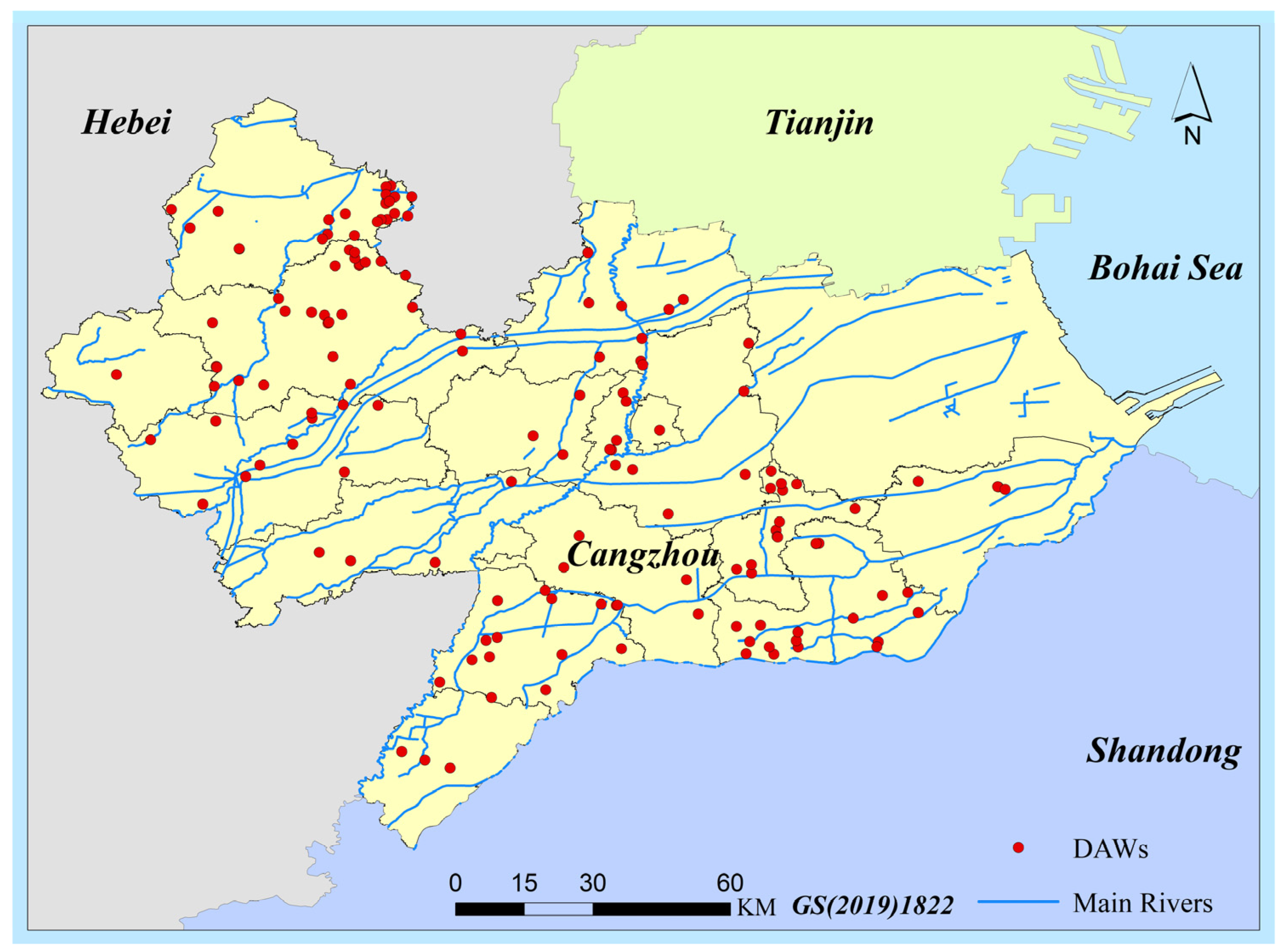
This study focuses on the Cangzhou region of Hebei Province as its research area, where black–odorous water bodies represent a critical yet challenging aspect of ecological environment remediation. As documented in the spatial distribution map of black–odorous water bodies issued by the Department of Natural Resources of Hebei Province, as shown in Figure 1, these polluted water masses predominantly originate from ponds, pits, and ditches receiving direct discharges of domestic wastewater, garbage, and livestock farming waste. These pollution sources trigger eutrophication processes that form black–odorous water conditions, characterized by extensive surface coverage of duckweed or algal blooms.

2.2. On-Site Sampling and Laboratory Analysis

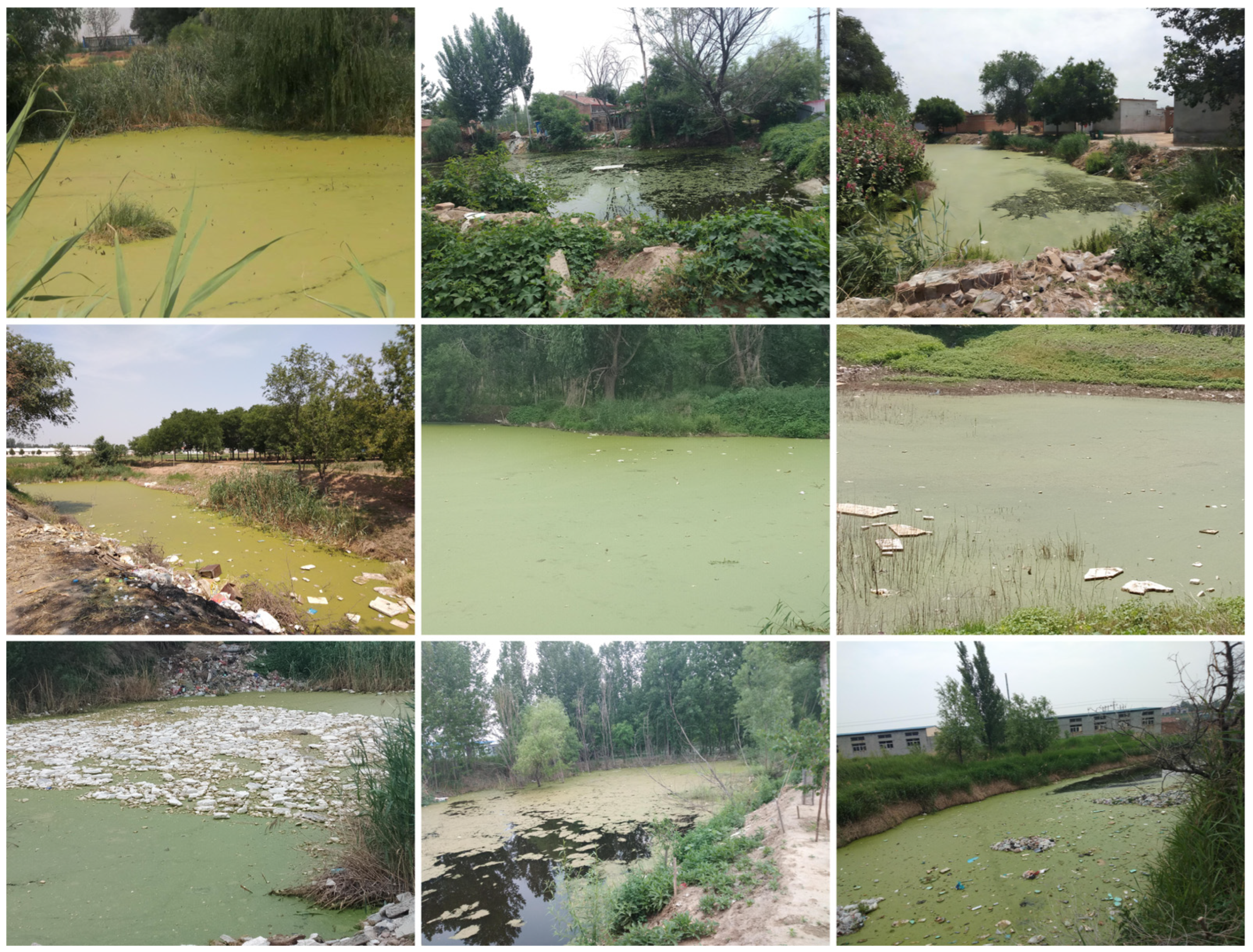
The in situ sampling of DAWs was conducted at 130 sampling points in Cangzhou from April 2022 to March 2025, and representative photographs are shown in Figure 2. Synchronously, a YSI ProPlus water quality analyzer(American Yellow Springs Instruments) was used to measure indicators including the dissolved oxygen (DO) and oxidation–reduction potential (ORP), and an ASD FieldSpec 4 Hi-Res spectroradiometer(From Longmont, CO, USA) was employed to collect spectral data (wavelength range: 350–2500 nm, covering all bands of the GF-2 satellite; sampling interval/resolution: 1 nm/3 nm for the 350–1000 nm range and 2 nm/8 nm for the 1000–2500 nm range). Measurements were strictly conducted between 10:00 and 14:00 (local time) under conditions of a stable solar altitude angle (30–60°), clear sky, and light wind (<Grade 3), with environmental parameters such as air temperature (20–28 °C) and relative humidity (40–60%) recorded; the water surface was required to be calm, and for sampling points with slight ripples, the average value of multiple measurements was adopted to offset reflection interference, while the spectroradiometer was calibrated using a white reference panel every 10 sampling points to eliminate instrument drift. A three-step method of “temporal–spatial synchronization–spectral resampling–reflectance correction” was used for matching with GF-2 images (time difference controlled within 1–3 days; GPS positioning for extracting the average reflectance of 3 × 3 pixels around each sampling point; Gaussian integration for resampling ASD continuous spectra to match GF-2 bands; and satellite reflectance calibration using ASD data with an average correction error < 3%). Collected water samples were transported to the laboratory under low-temperature refrigeration for the determination of the chemical oxygen demand (COD), ammonia nitrogen (NH₄⁺-N), and other indicators in accordance with relevant standards, which were used for validating the remote sensing identification model.

The remote sensing reflectance ($R_{rs}$) was derived based on Equation (1) [6]:

$$R_{rs}={\displaystyle \frac{L_u-p_f\times L_{sky}}{L_{blank}\times (\pi /P_{blank})}}$$

(1)

where $P_{blank}$ is the known reflectance factor of the spectral on the white reference panel used for calibration; $R_{rs}$ (remote sensing reflectance) is expressed in per steradian (${sr}^{-1}$); $L_u$ (upwelling radiance from the water surface), $L_{sky}$ (downwelling diffuse sky radiance), and $L_{black}$ (radiance of the white reference panel) all adopt the unit of Watts per square meter per steradian per nanometer ($W{m}^{-2}{sr}^{-1}n{m}^{-1}$); $L_f$ (sky light diffuse reflection coefficient), $\pi$ (circular constant), and $P_{blank}$ are dimensionless, with $P_f$ and $P_{black}$ ranging between 0 and 1. It should be noted that the units of the numerator ($L_u-P_f\times L_{sky}$) and denominator ($L_{black}\times (\pi /P_{blank}$)) are consistent, ensuring the dimensional consistency of the entire equation; after division, the radiometric dimensions cancel out, and only the angular unit ${sr}^{-1}$ is retained for $R_{rs}$, which conforms to its physical definition.

For water surfaces fully covered by duckweed or algal scum, where the spectrometer’s field of view is entirely occupied by aquatic vegetation or algae, the reflectance data were acquired using the methodology standard for terrestrial vegetation. The surface reflectance (SR) was calculated using Equation (2) [6,47]:

$$SR={\displaystyle \frac{L_u-P_{blank}}{L_{blank}}}$$

(2)

Herein, $p_f$ is the Fresnel reflection coefficient at the water surface. A constant value of 0.022 was adopted, which is standard for calm water conditions. Furthermore, subsurface water samples were obtained at a depth of 0.5 m to quantify the water quality parameters [47].

2.3. Satellite Imagery and Preprocessing

To clarify the details of the GF-2 images and ensure data reliability, 976 L1A-level GF-2 panchromatic + multispectral images (acquired during 2022–2025) covering the complete seasonal cycle of Cangzhou were obtained from the China Remote Sensing Satellite Application Center (CRSAS) (https://sasclouds.com/chinese/normal, accessed on 16 July 2025). The images were subjected to batch preprocessing using ArcGIS Pro (ESRI, Redlands, CA, USA), including radiometric calibration based on officially provided coefficients, FLAASH atmospheric correction (adopting mid-latitude seasonal profiles, the rural aerosol model, and water vapor retrieval from near-infrared bands), geometric precision correction referenced to a 1:10,000 digital elevation model (DEM) with a root-mean-square error (RMSE) < 0.5 pixels, and administrative boundary clipping. The image selection adhered to the “seasonal representativeness + quality priority” principle, covering the complete seasonal cycle of spring (recovery), summer (outbreak), autumn (decline), and winter (dormancy), with emphasis on the summer high-incidence period (accounting for 40%); extreme climate conditions were avoided, and the images were required to meet criteria including cloud cover <5%, no shadows or haze, and atmospheric visibility > 12 km to ensure stable spectral characteristics.

Four bands (blue, green, red, and near-infrared) were selected, and a preprocessing routine involving image standardization and normalization was implemented [47,48] in ArcMap to address the inter-scene variability in the radiometric response introduced by differing sun angles, seasonal conditions, and sensor calibrations. This critical step minimized color and brightness discrepancies, thereby enhancing the robustness of the subsequent analysis.

2.4. Training and Testing Sample Generation

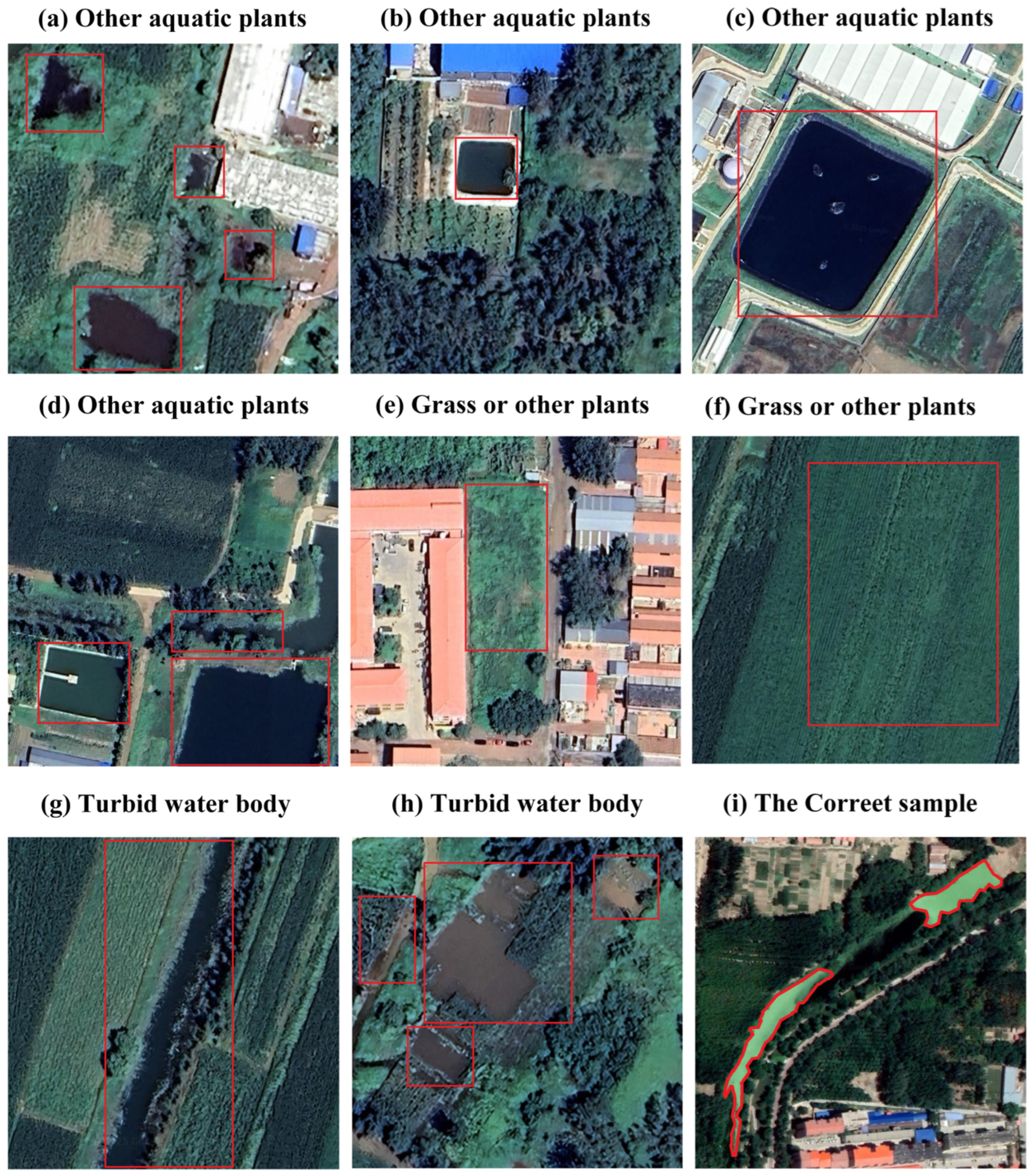
Given that the core distinction between DAWs and other land cover types (e.g., herbaceous plants, terrestrial vegetation, and other aquatic plants) lies in their color and texture characteristics [6,49], the selection of high-quality images as annotation basemaps was prioritized before sample labeling. To minimize subsequent annotation errors, the selected imagery needed to meet stringent quality standards, including uniform coloration and an absence of cloud cover and haze. During the annotation process, in addition to precisely delineating DAW boundaries, significant effort was devoted to removing easily confused noise samples (such as herbaceous plants, terrestrial vegetation, and other aquatic plants); representative examples are provided in Figure 3. The annotation task was performed by a team of trained specialists who manually delineated DAW boundaries in ArcGIS (ESRI, Redlands, CA, USA). Following the initial delineation, cross-verification and collaborative correction among the experts were conducted to ensure the accuracy of the final annotation.

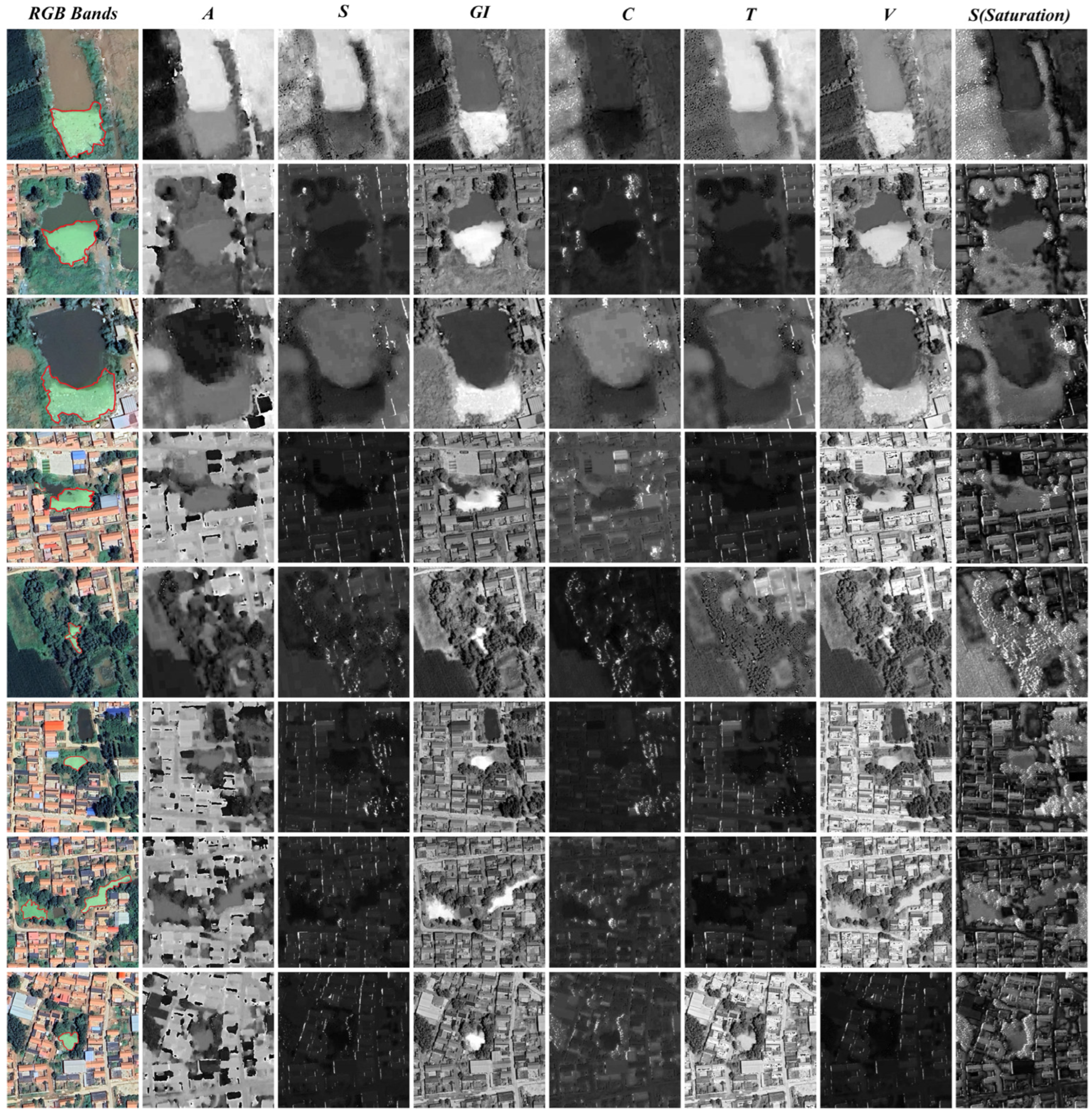
This study constructed a dedicated multi-feature remote sensing dataset for identifying black–odorous water bodies characterized by the presence of duckweed and algal scum. The sample generation process began with a rigorous screening of 0.8 m resolution remote sensing images to ensure accurate color representation and the absence of cloud obstruction. Subsequently, an innovative multidimensional feature set, the ASGICTVS, was developed and employed as the model inputs.

The methodology for feature engineering involved two sequential phases. First, the ASGI foundational features were derived from the RGB data to delineate basic spectral properties: the hue angle (α) for isolating color information, the Spectral Slope Composite Index (S) for modeling band relationships, and the Green Index (GI) for amplifying the vegetation signature. The CTVS feature set was engineered in the second phase to encapsulate specific water quality attributes. Herein, spectrally-derived indices for CDOM and turbidity were formulated via band ratios, thereby quantifying dissolved organic matter and suspended solids. Complementarily, the brightness and saturation components from the HSV color transformation were incorporated to characterize the luminance and chroma attributes of the water surface.

2.5. Remote Sensing Feature Enhancement Index

Based on the preceding in situ monitoring of black–odorous water body data in Cangzhou and analysis of the data characteristics of GF-2 high-resolution remote sensing imagery, this study argues that relying solely on the original image bands or existing general-purpose features makes it challenging to balance the identification accuracy and anti-interference capability. To address this issue, the ASGICTVS multidimensional feature set is constructed, whose core design philosophy adheres to the principle of “targeting the composite features of DAWs—fusing spectral, water quality, color and texture information—eliminating redundant features”. The composition of its core features is determined through a systematic screening process, which provides high-quality support for the subsequent feature input of the SwinTf-Unet model.

(a)

α—Hue Angle

The hue angle is a psychophysical measure obtained by transforming the CIE-XYZ color space [50]. It objectively quantifies the perceptual quality of hue, which is invariant to specific changes in illumination and intensity, unlike subjective descriptors like “bright green.” Represented as an angle (0° to 360°) on a chromaticity plane, it categorizes colors (e.g., red, green). The computation is shown as follows [51,52]:

$$\alpha =arctan 2(y-y_n,x-x_n)$$

(3)

(b)

S—Spectral Slope Composite Index

The formula for calculating the Spectral Slope Composite Index is shown in Formula (4) [50]:

$$S={\displaystyle \frac{B-G}{B+G}}+{\displaystyle \frac{R-G}{R+G}}$$

(4)

The first term, ${\displaystyle \frac{B-G}{B+G}}$, quantifies [53] the spectral slope differences between the blue-band absorption valley and green-band reflection peak, exhibiting high sensitivity to the concentration of chromophoric dissolved organic matter (CDOM) and water color deviation; the second term, ${\displaystyle \frac{R-G}{R+G}}$ [54], captures the spectral slope characteristics between the red-band absorption valley and green-band reflection peak, responding to variations in the algal chlorophyll content and suspended-solid concentration; the Composite Index enhances the discriminative capability between cyanobacterial blooms and clean water by synergistically leveraging dual spectral slope features, addressing the limitations of single-band ratio indices that are prone to interference.

(c)

GI—Green Index

The Green Index (GI) is defined by Formula (5) [50]:

$$GI={\displaystyle \frac{G^2}{B+R}}$$

(5)

This is calculated based on the visible light bands of GF-2 remote sensing imagery. Specifically, following the radiometric and atmospheric correction of GF-2 imagery, the surface reflectances of the blue (B), green (G), and red (R) bands in the target area are extracted. Subsequently, the intensity of green coverage of the target is quantitatively characterized through a ratio operation, where the sum of the blue- and red-band reflectances normalizes the square of the green-band reflectance. Its core identification mechanism resides in the fact that duckweed/algal bloom-dominated black–odorous water bodies (DAWs) are rich in chlorophyll, resulting in a significantly higher green-band reflectance compared to those for other land cover types. Consequently, the GI values of DAWs stably fall within the characteristic range of 1.8–2.5 (inclusive). In contrast, confusing land cover types, such as terrestrial vegetation and artificial lawns, exhibit GI values that deviate from this range (e.g., GI < 1.5 for synthetic lawns and GI > 2.8 for dense shrubs), attributed to differences in the pigment composition or coverage structure. Leveraging the high-spatial-resolution advantage of GF-2 imagery, the index accurately captures the green coverage signals of small and micro-scale duckweed/algal bloom patches. Meanwhile, the ratio-based calculation effectively mitigates interference from illumination fluctuations and background noise, providing a quantitative indicator for distinguishing DAWs from green-colored, confusing land cover types. This thereby addresses the challenge of precisely identifying green-covered targets in complex scenarios.

(d)

C—CDOM Index

The CDOM (Chromophoric Dissolved Organic Matter) Index [55,56] is defined by Formula (6):

$$CDOMI=1-{\displaystyle \frac{B}{G}}$$

(6)

In DAWs, chromophoric dissolved organic matter (CDOM) exhibits the strong absorption of short-wavelength blue light, resulting in a significant reduction in blue-band reflectance. In contrast, green-band reflectance remains relatively stable. This confines the CDOM Index to a characteristic range of 0.3–0.8, corresponding to a CDOM concentration of >20 mg/m³, which meets the water quality standard for “severe black–odorous water”. In contrast, clean water bodies have low CDOM concentrations, resulting in relatively high blue-band reflectance and CDOM Index values, which are mostly below 0.3. Confusing land covers, such as terrestrial vegetation and artificial surfaces, lacking CDOM-induced spectral absorption, exhibit inherent differences in the blue–green-band reflectance relationship compared to water bodies. Their CDOM Index values are either below 0.2 or above 0.9, forming a distinct boundary with DAWs. Leveraging the high-spatial-resolution advantage of Gaofen-2 (GF-2) remote sensing imagery, this index can accurately capture the characteristic of “blackening” in local water bodies. Meanwhile, the ratio-based calculation mitigates interference from illumination fluctuations and sensor noise, providing a highly robust quantitative indicator for identifying the “blackening” attribute of DAWs. This effectively addresses the challenge of accurately characterizing the blackness of water bodies in complex scenarios.

(e)

T—Turbidity Index

This metric is designed to quantify the concentration of suspended particles (e.g., sediment, organic detritus) in water bodies [57,58], defined by Formula (7):

$$TI={\displaystyle \frac{R}{G}}$$

(7)

Black–odorous water bodies (DAWs) are rich in suspended solids (SSs), such as algal debris and organic pollutant particles. These substances have a significant scattering-enhancing effect on red-band reflectance while exerting a weak scattering influence on green-band reflectance, resulting in the Turbidity Index stably falling within a characteristic range of 1.1–1.8. In contrast, clean water bodies have low SS concentrations, resulting in relatively low red-band reflectance and Turbidity Index values, which are mostly below 0.9. Confusing land covers (e.g., terrestrial vegetation and artificial surfaces), lacking SS-dominated scattering properties, display inherent differences in the red–green-band reflectance relationship compared to water bodies: terrestrial vegetation undergoes significant chlorophyll absorption in the red band, resulting in Turbidity Index values mostly below 0.8, while artificial surfaces (e.g., concrete pavements) exhibit abnormally high red-band reflectance, with index values typically exceeding 2.0. This forms a clear boundary with DAWs. Leveraging the high-spatial-resolution advantage of Gaofen-2 (GF-2) remote sensing imagery, this index can accurately capture the “turbidity” characteristic of local water bodies. Meanwhile, the ratio-based calculation mitigates interference from illumination fluctuations and sensor noise, providing a highly robust quantitative indicator for identifying the “turbidity” attribute of DAWs. This effectively addresses the challenge of accurately characterizing water body turbidity in complex scenarios.

(f)

Brightness (V) and Saturation (S)

These two indices quantify the “blackness” and “dimness” of water bodies from the perspective of human visual perception [59] and are defined by Formulas (8) and (9):

$$V=\mathrm{m}\mathrm{a}\mathrm{x} (R,G,B)$$

(8)

$$S=\left\{\begin{array}{rr}0,& if v=0\\ {\displaystyle \frac{V-\mathrm{m}\mathrm{i}\mathrm{n} (R,G,B)}{V}},& if v\ne 0\end{array}\right.$$

(9)

Black–odorous water bodies (DAWs) exhibit the visual characteristics of “dark tone and moderate color purity” due to the synergistic effects of high concentrations of chromophoric dissolved organic matter (CDOM), suspended solids (SSs), and duckweed/algal blooms. Specifically, the brightness (V) stably falls within the range of 0.2–0.4, corresponding to a dark tone resulting from the absorption and scattering of visible light, which induces low overall brightness. The saturation (S) remains steady in the range of 0.3–0.6, representing moderate saturation—attributed to the concentrated green-band reflectance peak (from duckweed/algal blooms) that fails to reach high purity due to scattering by impurities. In contrast, clean water bodies have high reflectivity and pale colors, with V values mostly above 0.5 and S values typically below 0.3. While some terrestrial vegetation (e.g., lawns, shrubs) overlaps with DAWs in V values (0.3–0.5), their S values are mostly above 0.6 owing to the pure green-band reflectance peak dominated by chlorophyll. Artificial surfaces (e.g., concrete pavements, red rooftops) exhibit characteristics of high V values (>0.6) or high S values (>0.7), forming a clear boundary with DAWs.

By synergistically leveraging the high-spatial-resolution advantage of Gaofen-2 (GF-2) remote sensing imagery, the V and S can accurately capture the details of the brightness and color purity of local water bodies. Meanwhile, the “maximum value/difference normalization” calculation mitigates interference from fluctuations in illumination intensity and sensor noise, providing a highly robust quantitative indicator for the visual attributes of “dark tone and moderate saturation” in DAWs. This effectively addresses the challenge of accurately characterizing the visual features of water bodies under complex illumination conditions. As the “visual feature dimension,” the V and S complement the Spectral Slope Composite Index (spectral feature) and CDOM/Turbidity Indices (water quality features), improving the “spectral–water quality–visual” three-dimensional feature recognition system of the ASGICTVS dataset. This significantly reduces the confusion probability between DAWs and interfering features, such as high- or low-light-affected surfaces and grayscale objects.

2.6. Experimental and Model Parameter Settings

This study adopted a strictly controlled experimental setup to ensure the comparability and reproducibility of the results. The experiments were conducted on a workstation equipped with an NVIDIA GeForce RTX 3090 GPU (24 GB VRAM, NVIDIA Corporation, Santa Clara, CA, USA), using a software environment based on Python 3.8 and the TensorFlow 2.1.2 framework. All input images were uniformly preprocessed to a resolution of 512 × 512 pixels and standardized. To enhance the model’s generalization ability, a comprehensive data augmentation strategy [60] was employed during training, including noise simulation enhancement, spectral feature enhancement, geometric distortion enhancement, and brightness/contrast enhancement, as detailed in

Table 1. ASGICTVS dataset enhancement methods.

Enhancement Operation Type	Specific Implementation Method	Design Purpose
Noise simulation enhancement	Adds Gaussian noise (variance range: 0.005–0.02) and salt-and-pepper noise (noise density: 0.01–0.03)	To simulate remote sensing sensor imaging noise and signal interference caused by atmospheric scattering to enhance the robustness of the model to low-quality images
Spectral feature enhancement	Spectral shifting (RGB-band reflectance ± 5–10% adjustment); spectral stretching (spectral contrast optimization based on histogram equalization)	To simulate spectral variations caused by different atmospheric correction accuracies, lighting conditions (such as cloudy/sunny days), and seasonal variations to enhance the adaptability of the model to spectral differences
Geometric distortion enhancement	Random cropping (cropping ratio: 0.7–1.0); elastic deformation (deformation coefficient: 0.1–0.3)	To adapt to scenes with irregular water boundaries and distorted local areas (such as geometric distortions caused by terrain undulations) in remote sensing images to enhance the segmentation generality
Brightness/contrast Enhancement	Brightness adjustment (±10–15%); contrast adjustment (±15–20%)	To simulate changes in image brightness caused by differences in atmospheric transparency during different shooting periods (morning/afternoon/evening) to avoid relying on a single brightness feature for model recognition

.

The model employs the SwinTf-Unet architecture, where Swin-Tiny was pre-trained on the ImageNet dataset to provide the initial encoder weights. The optimization process used the AdamW optimizer with an initial learning rate of 1 × 10⁻³ and a weight decay coefficient of 1 × 10⁻⁴, configured for a total of 150 epochs to achieve more stable convergence. To address the class imbalance problem between DAWs and background pixels, the loss function utilized an equal-weighted combination of Dice loss and Focal loss. The training batch size was set to 8, with a maximum of 100 training epochs, and an early stopping mechanism (patience = 10) was introduced to prevent overfitting.

2.7. Accuracy Evaluation

The performance of different semantic segmentation networks was evaluated by computing and comparing the following metrics: the precision, recall, F1-score, and IoU. These metrics comprehensively assess the models’ accuracy, robustness, and segmentation quality:

$$Precision=TP/(TP+FP)$$

(10)

$$Recall=TP/(TP+FN)$$

(11)

$$F1-score={\displaystyle \frac{2}{\frac{2}{Precision}+\frac{1}{Recall}}}={\displaystyle \frac{2TP}{FP+2TP+FN}}$$

(12)

$$IoU={\displaystyle \frac{TP}{TP+FP+FN}}$$

(13)

The positive (P) is defined as the target category (DAWs), and the negative (N) refers to the non-target category (e.g., clean water, green confounding features, bare land, buildings). The four core binary classification metrics are defined as follows: true positive (TP)—the number of pixels correctly identified as DAWs; false positive (FP)—the number of non-DAWs pixels incorrectly classified as DAWs (false alarm); false negative (FN)—the number of DAWs pixels incorrectly classified as non-DAWs (miss detection); true negative (TN)—the number of non-DAWs pixels correctly identified as non-targets.

When evaluating the model’s ability to recognize black–odorous water, the overall accuracy (OA), false-positive rate (FPR), and false-negative rate (FNR) are used as evaluation metrics:

$$OA=(TP+TN)/(P+N)$$

(14)

$$FPR=FP/(TN+FP)$$

(15)

$$FNR=FN/(TP+FN)$$

(16)

The complexity of the model is determined by the number of model parameters, which represent the explicit memory required by the model. It calculates the total number of parameters by adding all the parameters that need to be learned in the model. The evaluation index for the total number of parameters in this article is represented by the parameter (MB).

2.8. The Structure of the SwinTf-Unet

This study employed the Swin Transformer as the encoder to extract features from DAWs. At the same time, the U-Net served as the decoder to reconstruct the segmentation results.

2.8.1. Swin Transformer Model Structure

The window attention mechanism provides key support for the remote sensing identification of DAWs (duckweed/algal bloom-dominated black–odorous water bodies): the hierarchical design can generate multi-scale feature maps, accommodating the scale differences between “small targets (duckweed/algal blooms) and large-scale water bodies”; the shifted window mechanism reduces the computational complexity to a linear level, enabling the efficient processing of GF-2 high-resolution images while achieving modeling of global spatial dependencies through cross-window information interaction.

The specific application methods were tailored to the task requirements:

(1)

Optimization of the window size to 4 × 4, enhancing the ability to capture the features of scattered, small-area duckweed/algal blooms;

(2)

Embedding the ASGICTVS feature dimension during the encoding process, integrating vegetation, water quality, and visual features into the attention calculation to strengthen the target spectral discriminability and suppress background interference;

(3)

Adjustment of the shifted window stride to adapt to the irregular spatial distribution of water bodies and reduce cross-regional feature confusion.

This encoder not only retains the global modeling advantage of Transformers but also addresses the shortcomings of pure Transformers in remote sensing small-target identification through task-specific parameter adjustments, providing highly discriminative multi-scale features for the decoder.

2.8.2. The Unet Model Structure

As a classical segmentation network, the U-Net employs a symmetric U-shaped architecture to achieve semantic segmentation by extending and modifying fully convolutional networks [31]. The entire network is divided into an encoder and a decoder. The encoder progressively downsamples the input, reducing spatial dimensions to extract features, while the decoder stepwise restores spatial dimensions and details to facilitate image reconstruction.

In this study, the U-Net was employed as the decoder component of the Swin-Unet model to restore spatial resolution from the high-level features extracted by the Swin Transformer and accurately segment DAWs. Through skip connections, the U-Net integrates low-level features from various encoder layers with upsampled features in the decoder, effectively preserving detailed information and enhancing the segmentation accuracy. Ultimately, the output layer of the U-Net generates a segmentation map of the exact dimensions as the input image, precisely distinguishing DAWs from the background. This approach offers a high-precision, automated method for monitoring water bodies in complex environments. The model structure is shown in Figure 4.

3. Results

3.1. Optical Properties of DAWs in Remote Sensing Imagery

The reflectance of water bodies is governed by their inherent optical properties, which are determined by the concentration and composition of their constituent materials. These compositional differences manifest as distinct optical characteristics, which are further reflected in variations in water color and spectral reflectance profiles, as shown in the quantitative statistical results presented in

Table 2. Statistical results of spectral reflectances for different water types and features (mean ± standard deviation).

Band	Clear Water	Turbid Water	Eutrophic Water	Duckweed/ Algal Bloom-Type DAWs	Artificial Lawn (Terrestrial Feature)	CDOM-Rich Water
Blue (440–500 nm)	0.04 ± 0.01	0.08 ± 0.01	0.06 ± 0.01	0.07 ± 0.01	0.10 ± 0.02	0.05 ± 0.01
Green (520–580 nm)	0.06 ± 0.01	0.18 ± 0.03	0.15 ± 0.02	0.21 ± 0.03	0.22 ± 0.03	0.12 ± 0.02
Red (620–680 nm)	0.03 ± 0.01	0.15 ± 0.02	0.08 ± 0.01	0.09 ± 0.01	0.18 ± 0.02	0.08 ± 0.01
Near-Infrared (770–890 nm)	0.02 ± 0.005	0.10 ± 0.02	0.07 ± 0.01	0.05 ± 0.01	0.65 ± 0.05	0.04 ± 0.01
${\displaystyle \frac{Rg}{Rr}}$	2.00 ± 0.15	1.20 ± 0.12	1.88 ± 0.18	2.33 ± 0.21	1.22 ± 0.13	1.50 ± 0.16
Peak Reflectance Wavelength (nm)	500 ± 10	580 ± 15	550 ± 12	540 ± 10	550 ± 10	530 ± 12

. In clear water bodies, the reflectance remains relatively low across the spectrum, with mean values of 0.04 ± 0.01, 0.06 ± 0.01, 0.03 ± 0.01, and 0.02 ± 0.005 in the blue (440–500 nm), green (520–580 nm), red (620–680 nm), and near-infrared (770–890 nm) bands of the GF-2 satellite, respectively, and the highest values typically observed within the 400–600 nm range. Turbid water bodies exhibit significantly elevated reflectance in the 550–650 nm region due to strong scattering by suspended sediments, with mean reflectances of 0.18 ± 0.03 in the green band and 0.15 ± 0.02 in the red band—3.0 and 5.0 times higher than those of clear water, respectively. Eutrophic waters, influenced by phytoplankton pigments, often display a prominent reflectance peak near 550 nm induced by chlorophyll a, with the green-band reflectance (0.15 ± 0.02) being 2.5 times that of clear water and the red-band reflectance (0.08 ± 0.01) remaining relatively low. Overall, water bodies generally exhibit low reflectance levels compared to terrestrial features (e.g., artificial lawns, with mean reflectances of 0.22 ± 0.03 in the green band and 0.18 ± 0.02 in the red band).

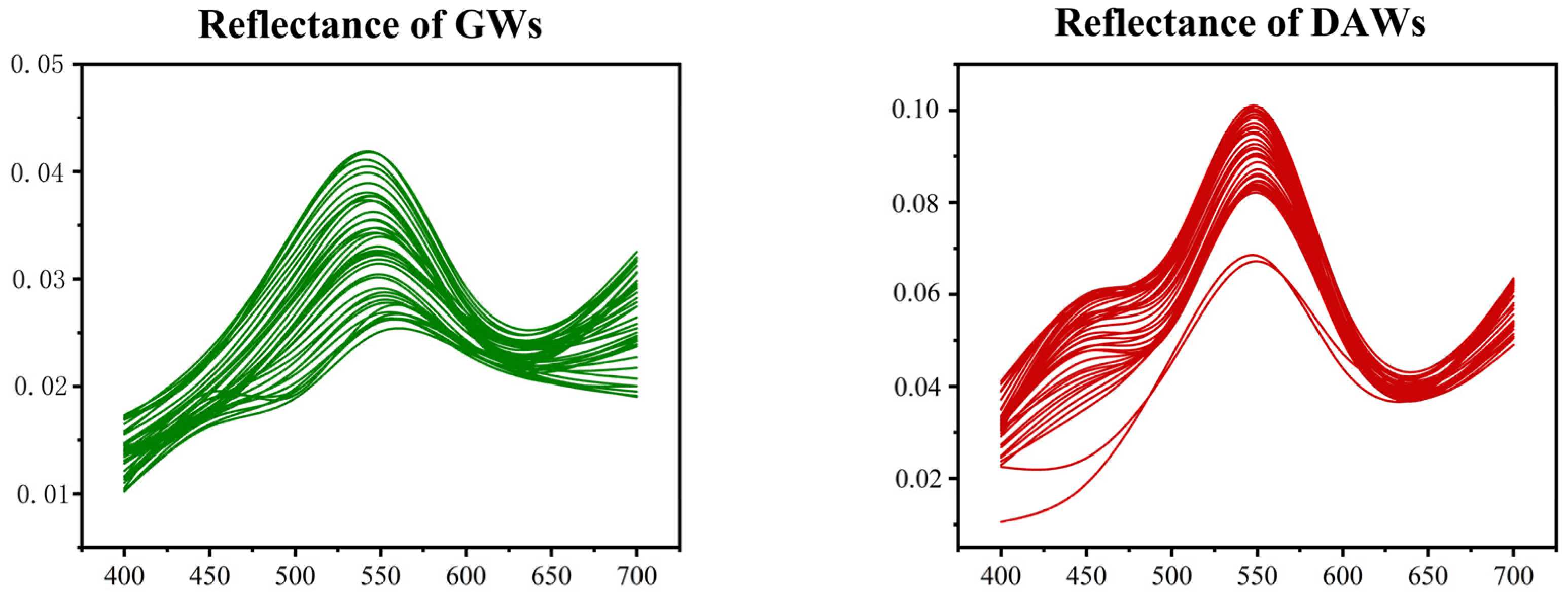
For DAWs, the spectral reflectance exhibits distinct statistical characteristics: the mean reflectance in the green band reaches 0.21 ± 0.03, which is 3.5 times higher than that of clear water, 1.2 times higher than that of turbid water, and 1.4 times higher than that of eutrophic water; the blue-band reflectance is 0.07 ± 0.01 (1.75 times that of clear water), the red-band reflectance is 0.09 ± 0.01 (3.0 times that of clear water), while the near-infrared-band reflectance is 0.05 ± 0.01 (2.5 times that of clear water). The reflectance peak of DAWs is concentrated at 530–560 nm (green band), with a mean peak reflectance of 0.23 ± 0.03, which is the key optical signature distinguishing them from other water types. Additionally, the ratio of the green-band-to-red-band reflectance (${\displaystyle \frac{Rg}{Rr}}$) for DAWs is 2.33 ± 0.21, significantly higher than those of clear water (2.00 ± 0.15), turbid water (1.20 ± 0.12), and eutrophic water (1.88 ± 0.18), providing a quantitative indicator for DAW identification.

Dissolved and particulate organic matter (commonly categorized as colored dissolved organic matter—CDOM) demonstrates spectral response characteristics that may resemble those of aquatic or terrestrial vegetation, with a mean green-band reflectance of 0.12 ± 0.02 and ${\displaystyle \frac{Rg}{Rr}}$ of 1.50 ± 0.16—lower than those of DAWs. In the visible spectrum, the spectral properties of vegetation are primarily governed by photosynthetic pigments, with chlorophyll being the dominant factor. Chlorophyll strongly absorbs radiation in the blue (around 450 nm; mean reflectance: 0.05 ± 0.01) and red (around 650 nm; mean reflectance: 0.06 ± 0.01) spectral regions while exhibiting lower absorption in the green area (approximately 540 nm; mean reflectance: 0.22 ± 0.03), resulting in a characteristic reflectance peak. This absorption mechanism similarly explains why most DAWs appear green in visible observations, with their spectral characteristics quantitatively consistent with the chlorophyll-dominated absorption–reflection pattern as shown in Figure 5 and Table 2.

3.2. Water Quality Characteristics of DAWs in Cangzhou

Statistical analysis of the classification results across the entire Cangzhou study area (total area: 14,304.26 km²) showed that the total area of duckweed/algal bloom-type black–odorous water bodies (DAWs) was 4.86 km², accounting for 0.034% of the study area. Spatially, the DAWs were mainly distributed in rural ditches (2.60 km², accounting for 53.5% of the total DAW area) and small ponds (2.01 km², 41.3%), while only 0.25 km² (5.2%) was distributed in urban small water bodies. Seasonally, the area of the DAWs peaked in summer (2.16 km², 44.4%) and reached the minimum in winter (0.54 km², 11.2%), which is consistent with the growth cycle of duckweed/algae.

DAWs are typically in a state of severe eutrophication and anaerobiosis in Cangzhou. Extremely high concentrations of nutrients such as nitrogen and phosphorus provide favorable conditions for the explosive growth of algae and duckweed. The dense biological coverage severely limits light penetration into the water column, while dissolved oxygen is rapidly depleted, creating hypoxic to anoxic conditions. Under these circumstances, the anaerobic decomposition of organic matter generates malodorous gases such as hydrogen sulfide and ammonia. In contrast, heavy metals such as iron and manganese are reduced and released, resulting in the darkening and odorization of the water. Water quality monitoring indicators reveal extremely low dissolved oxygen concentrations (often below 2 mg/L), elevated ammonia nitrogen levels, reduced transparency, and sharply decreased oxidation–reduction potential (ORP). Collectively, these characteristics indicate the collapse of ecosystem functioning, classifying the quality of such water bodies as typical inferior Class V water quality.

3.3. Selection of Enhanced Remote Sensing Features

The chromatic angle effectively distinguished DAWs from features such as verdant vegetation and artificial structures, including blue and green rooftops. The α values of the DAWs were primarily concentrated within the range of 181.5–182.2°. In comparison, verdant vegetation (181.0–181.7°) and red rooftops (179.5–180.3°) exhibited generally lower α values, whereas blue rooftops (182.0–183.0°) and green rooftops (182.6–183.3°) displayed significantly higher α values. Among these, the distinction between DAWs, red, and green rooftops was the most pronounced, as shown in Figure 6.

The Spectral Slope Composite Index effectively discriminated DAWs from dark-green vegetation. The S values of the DAWs were consistently distributed within the range of 1.2–1.7, whereas those of dark-green vegetation were mainly below 1.2 or above 1.7. This parameter thus provides an essential spectral basis for distinguishing between the two classes.

The Green Index strongly distinguished DAWs from sparse grasslands, green water bodies, and artificial turf. The GI values of the DAWs were mainly concentrated between 100 and 140, whereas those of sparse grasslands, green water bodies, and artificial turf were generally below 100. This makes the GI an effective indicator for suppressing interference from confounding land cover types.

The CDOM Index significantly enhanced the separability between DAWs and clean water bodies. Due to their high contents of colored dissolved organic matter, the DAWs typically exhibited CDOM Index values below 0.6, whereas clean water bodies generally showed values above 0.8. This parameter thus provides critical optical evidence for identifying black–odorous conditions in water bodies.

The Turbidity Index effectively differentiated turbid-type black–odorous water bodies from those dominated by CDOM. DAWs with high suspended-particulate contents typically exhibited Turbidity Index values above 1.1, whereas CDOM-dominated DAWs generally had values below 0.9. This feature provides a new dimension for analyzing the internal composition of black–odorous water bodies.

The brightness feature demonstrated a notable advantage in identifying DAWs. Due to strong light absorption, the DAWs generally exhibited brightness values below 40 (on a 0–255 scale), considerably lower than those of bright surface features such as bare soil or buildings, which typically exceeded 120. This makes brightness a key parameter for rapidly detecting dark-colored water bodies.

The saturation effectively captured the color degradation characteristics of DAWs. The DAWs’ saturation values were mainly below 0.3 (in the HSV color space), whereas those of healthy vegetation and artificial colored surfaces generally exceeded 0.5. This feature clearly reflects the visual characteristic of black–odorous water bodies as “dark and turbid”.

3.4. Model Training Convergence, Data Augmentation Optimization, and Cross-Validation Results

Data augmentation encompasses four types of targeted enhancement operations tailored to remote sensing images: noise simulation, spectral feature adjustment, geometric distortion, and brightness/contrast modification. A composite augmentation framework of “basic transformation + remote sensing feature adaptation” was established, expanding the sample size to 4 times that of the original ASGICTVS dataset. The key performance metrics were significantly improved compared with those before data augmentation: the IoU increased from 72.3% to 83.46%, the precision rose from 80.1% to 87.5%, and the recall improved from 82.4% to 88.41%. These results demonstrate that the newly added enhancement operations effectively enhance the model’s adaptability to complex variation scenarios in remote sensing images and mitigate the overfitting risk induced by limited samples.

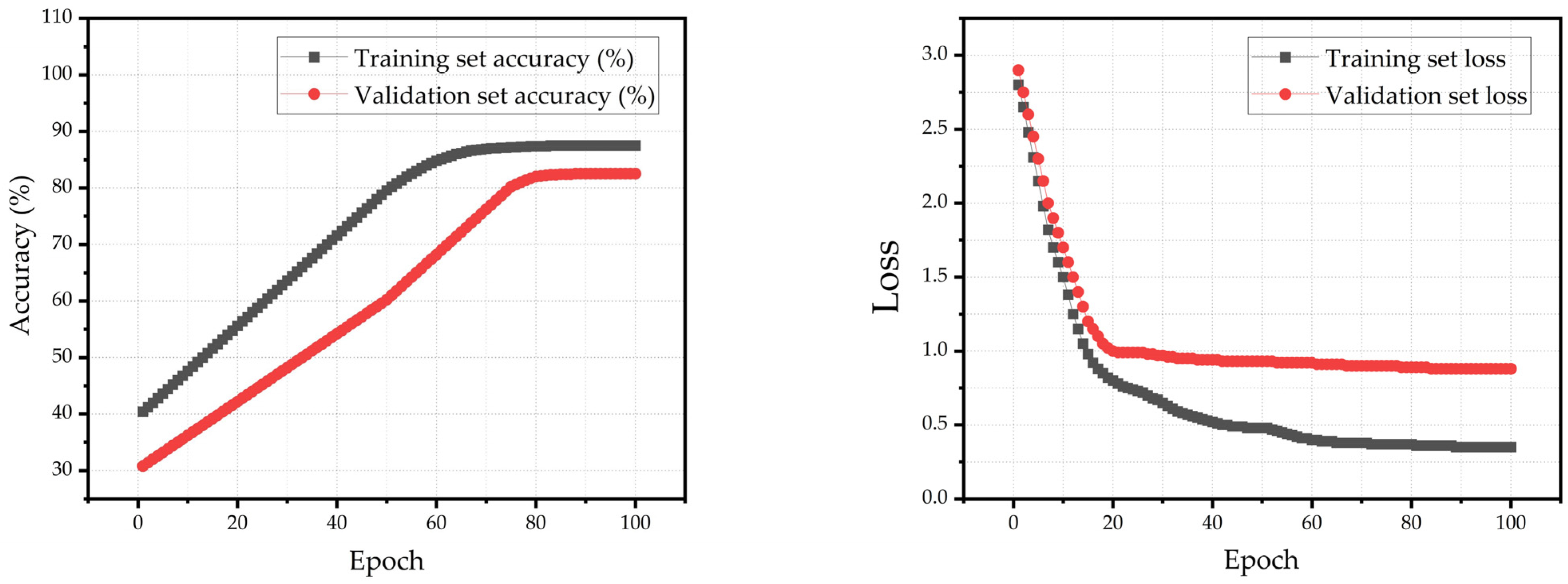
To further verify the model’s generalization ability, 5-fold cross-validation was employed. A total of 21,104 samples were randomly partitioned into five groups, where each group alternated as the test set and the remaining four groups were used as the training set for iterative validation. Based on the training protocol of the “AdamW optimizer + early stopping mechanism (patience = 10, monitoring validation loss)”, the model achieved stable convergence after 100 epochs of iteration. The optimal results from the 5-fold cross-validation are illustrated in Figure 7. The training loss gradually decreased from an initial value of 2.80 to 0.35, exhibiting an overall trend of “rapid decline followed by slow convergence”: a 78.6% reduction was observed in the first 20 epochs (from 2.80 to 0.80), and the model entered a stable phase after 60 epochs with a fluctuation range ≤0.02. The validation loss decreased from 2.90 to 0.88 and then remained stable without any upward tendency, thereby preventing overtraining. In terms of accuracy, the validation accuracy increased to 82.5%, and the training accuracy reached 87.5%. This indicates that the model suffered no underfitting or obvious overfitting, and the training process was stable and reliable.

4. Discussion

4.1. Effectiveness of Various Input Features for SwinTf-Unet

This section presents a comparative analysis of the effects exerted by raw RGB inputs, ASGI inputs, and the ASGICTVS super feature set on the precision of the SwinTf-Unet model, as illustrated in

Table 3. Testing accuracies of two input methods.

Input	Precision (%)	Recall (%)	F1-Score (%)	IoU (%)
RGB	62.41	57.63	72.46	63.90
ASGI	76.82	71.26	82.62	69.84
ASGICTVS	87.50	88.41	85.32	83.46

.

The ASGICTVS dataset demonstrated comprehensive superiority over the SwinTf-Unet model, significantly outperforming results achieved using only RGB or ASGI features. This strongly validates the effectiveness of its multi-feature fusion strategy, with advantages primarily manifested in the following three aspects:

(a)

Complementarity of multidimensional features enhances model discriminative power.

The ASGICTVS dataset integrates eight features from three categories: phenological color features (chromatic angle (α); slope mixture (S); Green Index (GI)); water quality parameters (CDOM Index; Turbidity Index); and visual perception features (brightness (V); saturation (S)). This combination enables the model not only to identify surface green biological coverage through the ASGI but also to penetrate the surface and sense the optical pollution characteristics of the underlying water via the CDOM and Turbidity Indices while capturing its “dark, turbid, and black” visual traits through brightness and saturation. Such multi-perspective feature complementarity substantially enriches the model’s discriminative basis.

(b)

Effective suppression of complex background interference, improving extraction accuracy.

The newly added CTVS features (CDOM, turbidity, brightness (V), saturation (S)) were specifically designed to capture the characteristic “low reflectance, high absorption, and dark coloration” of black–odorous water bodies. Brightness (V) and saturation (S) effectively eliminate high-reflectance or vividly colored confounding surfaces, such as colored rooftops and bare soil. At the same time, the CDOM and Turbidity Indices distinguish DAWs from clean water bodies and ordinary vegetation, which have differing optical properties. This explains the substantial improvement in the precision (87.50%) and IoU (83.46%), indicating fewer misclassifications and the more accurate delineation of water body boundaries.

(c)

Deep compatibility with the SwinTf-Unet architecture, fully leveraging global modeling advantages.

The global attention mechanism of the SwinTf-Unet efficiently processes and integrates the multi-channel, multi-scale information provided by the ASGICTVS. The model can self-learn the weighting relationships among different feature channels, for instance, by simultaneously considering the GI, which represents vegetation, and the CDOM Index, which represents black–odorous characteristics, thereby accurately localizing “covered black–odorous water bodies”. This contributes to the notable improvement in the recall (88.41%) and F1-score (85.32%) under complex scenarios, enabling more comprehensive target detection and reducing omissions.

In summary, the ASGICTVS dataset, by integrating multi-source optical indices, constructs a more comprehensive and physically meaningful feature space, enabling the SwinTf-Unet model to transition from “identifying green coverage” to “diagnosing black–odorous water quality”. This approach achieves higher precision and the end-to-end extraction of duckweed- or algal bloom-covered black–odorous water bodies.

4.2. Ablation Study of SwinTf-Unet Modules

An ablation study was conducted to evaluate the contribution of the individual modules within the SwinTf-Unet architecture to the overall model performance. Key components, including the Swin Transformer encoder, multi-scale feature fusion, and skip connections, were systematically removed or modified to assess their impact on the classification accuracy and feature extraction capabilities. Performance metrics, including the precision, recall, F1-score, and IoU, were compared across ablated and full models to quantify the significance of each module. The results as shown in

Table 4. Results of the model ablation experiment.

Model	Input	Encoder	Precision (%)	Recall (%)	F1 (%)	IoU (%)
Model A (Baseline)	RGB	ResNet-50	75.21	70.58	72.80	57.15
Model B	ASGICTVS	ResNet-50	81.62	77.29	74.30	69.28
Model C	RGB	SwinTf-Unet	81.55	83.70	82.61	70.12
Model D (Our Model)	ASGICTVS	SwinTf-Unet	87.50	88.41	85.32	83.46

reveal which architectural elements are essential for capturing surface green coverage and underlying water quality characteristics, providing insights into the model’s robustness and the effectiveness of its global–local feature modeling.

Model A (baseline): U-Net with ResNet-50 encoder + RGB input;

Model B: U-Net with ResNet-50 encoder + ASGICTVS input;

Model C: SwinTf-Unet (Swin Transformer as encoder) + RGB input;

Model D (our full model): SwinTf-Unet (Swin Transformer as encoder) + ASGICTVS input.

(a)

Contribution of Input Features (Model A vs. Model B)

Performance Improvement: Replacing the input from the RGB to AGICTVS feature set, while keeping the ResNet-50 encoder unchanged, resulted in a significant increase across all metrics (e.g., the F1-score rose from 72.80% to 74.30%, and the IoU increased from 57.15% to 69.28%).

Conclusion: The ASGICTVS feature set is a crucial factor in enhancing performance. The multidimensional optical, chromatic, and water quality features it provides substantially improve the model’s ability to distinguish the target from complex backgrounds, validating the effectiveness of its design.

(b)

Contribution of the Encoder (Model A vs. Model C)

Performance Improvement: Merely replacing the encoder from ResNet-50 to the Swin Transformer, while maintaining the same RGB input, also led to a substantial performance boost (e.g., the F1-score increased from 72.80% to 82.61%, and the IoU improved from 57.15% to 70.12%).

Conclusion: The Swin Transformer encoder itself constitutes a more powerful feature extractor. Its robust global context modeling capability enables a superior understanding of the scene and the capture of long-range dependencies, even when using only RGB input, thereby reducing false positives and negatives.

(c)

Synergistic Effect of the Complete Model (Model D)

Performance: Our complete model (Swin Transformer + ASGICTVS) achieved the optimal performance (F1: 85.32%; IoU: 83.46%).

Conclusion: A significant synergistic effect exists between the SwinTf-Unet architecture and the ASGICTVS feature set, demonstrating a scenario where the combined effect is greater than the sum of its parts. The Swin Transformer’s powerful global modeling capability fully exploits and integrates the rich physical information embedded within the ASGICTVS features. Conversely, the distinct and highly separable features provided by the ASGICTVS supply the Swin Transformer with superior learning material. This synergistic combination facilitates a significant leap from merely seeing the targets to truly understanding them.

4.3. Comparison of SwinTf-Unet Model Performance with Existing Models

To comprehensively evaluate the advanced nature of the proposed SwinTf-Unet model, we conducted a comprehensive comparative evaluation against state-of-the-art semantic segmentation models currently used for DAW extraction, including the SEM-Unet [6], EAF-Unet [61], DeepLabV3+ [62], the MobileViT-UNet [63], SegViT [64], and the SAM-based segmentation model [65], as shown in

Table 5. Comparison table of evaluation indicators for different semantic segmentation networks.

Model	Encoder Backbone Architecture	Precision (%)	Recall (%)	F1-Score (%)	IoU (%)	Floating-Point Computational Load (G FLOPs)	Reasoning Time (ms/Sheet)
EAF-Unet	ResNet-101 + ECA	80.11	78.91	79.52	65.97	35.6	25.8
DeepLabV3+	Xception	82.32	81.03	81.79	68.94	68.9	32.5
SEM-Unet	MobileNetV2 + scSE	83.92	82.63	81.96	69.75	28.2	27.3
MobileViT-UNet	MobileNetV2	79.22	77.41	73.97	71.60	31.8	28.3
SegViT	ViT	74.17	70.63	72.06	72.49	105.4	65.8
SAM-based segmentation model	ViT	84.26	82.92	79.18	73.06	280.7	125.7
SwinTf-Unet (our model)	Swin- Transformer	87.50	88.41	85.32	83.46	38.7	31.2

The bold numbers in the table represent the optimal accuracy indicators.

. To ensure a fair and rigorous comparison, all models were trained and tested under identical conditions, utilizing the same dataset (ASGICTVS) and identical training configurations.

The results demonstrate that the proposed SwinTf-Unet model significantly outperforms all existing comparative models across all key accuracy metrics. Section 4 details its exceptional performance in DAW extraction.

(a)

Comprehensive Superiority in Accuracy Performance

Table 5 presents the core accuracy metrics of multiple semantic segmentation models for DAW identification. Our SwinTf-Unet shows distinct comprehensive advantages across the precision, recall, F1-score, and IoU (the four key indicators): its precision (87.50%) is 3.53 percentage points higher than the second-ranked SEM-Unet (83.97%), indicating fewer false favorable judgments for confounding features (e.g., green rooftops); the recall (88.41%) is 7.34% higher than that for DeepLabV3+ (81.07%), reflecting a lower omission rate for small, scattered DAW patches. The F1-score (85.32%) (the harmonic mean of the precision and recall) verifies the model’s balanced performance between reducing misjudgments and omissions. As the core segmentation metric, the IoU (83.46%) is 14.56% higher than that of DeepLabV3+ (68.90%), directly demonstrating that its segmentation results align more closely with the proper distribution of DAWs.

The SwinTF-Unet’s FLOPs are higher than those of the lightweight model SEM-Unet, and the inference speed can still reach 31.2 ms/image, meeting the “quasi-real-time” requirements for the large-scale monitoring of black–odorous water bodies (the coverage area of a single satellite image is about tens of square kilometers, including thousands of 512 × 512 sub blocks, and the processing time of the entire image can be controlled within minutes).

(b)

Exceptional Detail Preservation Capabilities

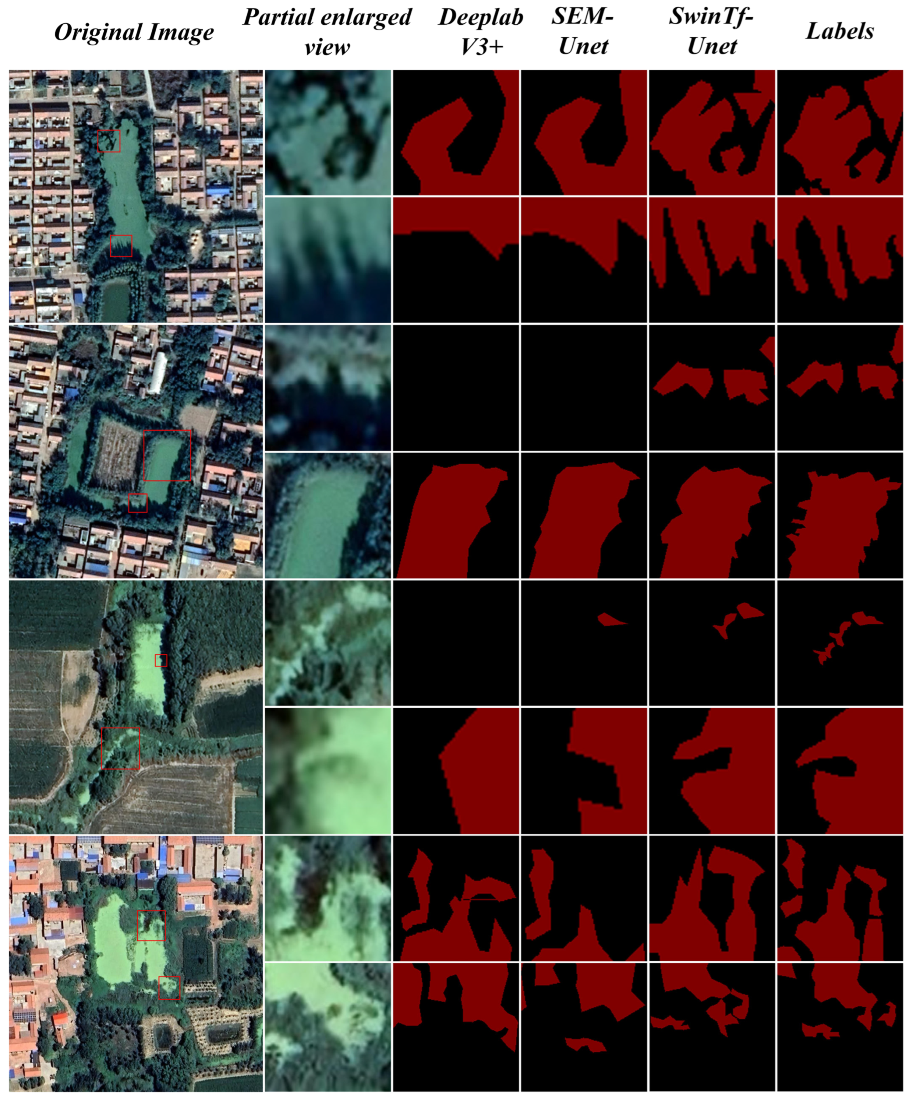
The SwinTf-Unet model exhibits remarkable advantages in capturing the dynamic shape variations in DAWs, achieving higher fitting accuracy, especially for complex contour details such as water body corners, as shown in Figure 8. This advantage further confirms the model’s excellent detail preservation capability—the natural morphology of DAWs often presents irregular corners due to tortuous shorelines and occlusion by aquatic plants, water flow impacts, and other factors. Traditional segmentation models are prone to issues such as contour smoothing, breakpoints, or overfitting in such areas due to the limitations of local receptive fields or feature dilution effects. In contrast, the SwinTf-Unet enhances the capture of local features by utilizing a customized 4 × 4 window size. By integrating the multi-scale feature skip connection strategy of the decoder, it accurately anchors pixel-level contour variations at corners, resulting in segmentation results that are highly consistent with the actual morphology of water bodies. This can be intuitively verified in the locally enlarged views of Figure 8, particularly in the corner regions.

(c)

Advantages in Visual Comparison

In the visual results, the advantages of the SwinTf-Unet are particularly evident:

Reduction in False Positives: Comparative models (especially the EAF-Unet and DeepLabV3+) frequently misclassify green roofs, artificial turf, or shadows as DAWs. In contrast, leveraging its global reasoning capability and the rich spectral information provided by the ASGICTVS input, the SwinTf-Unet effectively suppresses such background interference.

Reduction in False Negatives: For DAWs that are partially occluded, extremely small in area, or have blurred edges, other models are prone to missed detections. The global perceptual field of view of the SwinTf-Unet ensures that it can “see” and identify these challenging samples.

Boundary Integrity: The water contours extracted by the SwinTf-Unet are smoother and more complete, whereas the outputs of comparative models may exhibit holes or irregular edges.

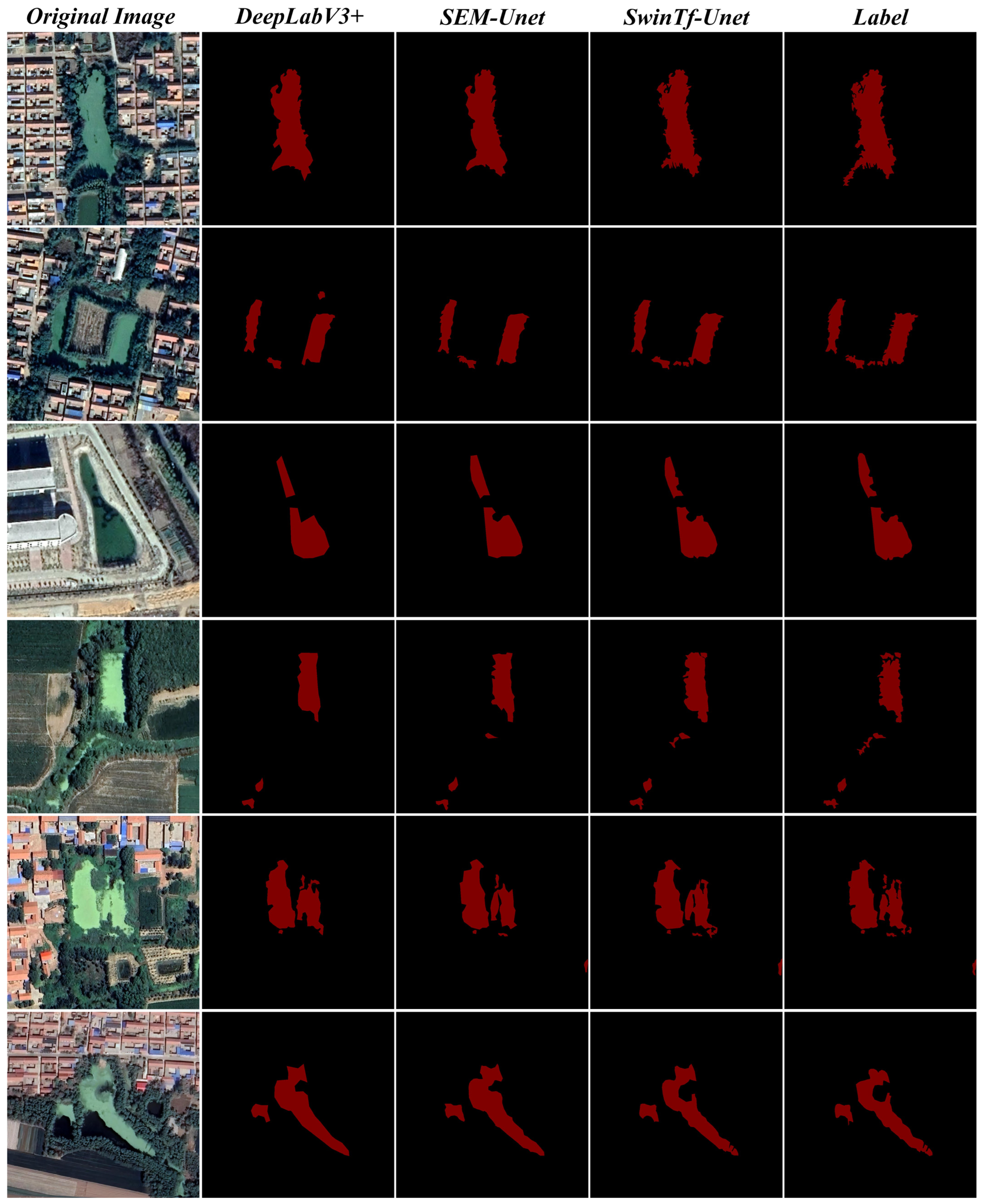
In summary, the SwinTf-Unet represents a model with increased parameters and enhanced performance, signifying a fundamental generational leap in architectural design. It successfully adapts the global modeling capabilities of Transformers, originally prominent in natural language processing, to visual segmentation tasks, while ingeniously addressing computational complexity through its shifted window mechanism. This study’s specific task of DAW extraction demonstrates remarkable superiority over existing state-of-the-art CNN-based models, as shown in Figure 9. By achieving comprehensive improvements in the precision, recall, and segmentation detail while maintaining a reasonable parameter count, it establishes a new benchmark for remote sensing feature extraction in complex environments.

(d)

Limitations and improvement directions of models in complex environments

The SwinTf-Unet model proposed in this study exhibits high accuracy in identifying the core regions of black–odorous water bodies (DAWs). Still, it has certain limitations in complex environments, such as shadow interference and mixed water body boundaries. In shadow-covered areas (e.g., vegetation or building shadows), the DAW recognition accuracy decreases from 87.5% in shadow-free regions to 69.7%, prone to misclassifying shadow-covered clean water as mild DAWs or DAWs at shadow edges as non-DAWs. The underlying causes include the shadow-induced suppression of spectral features, disruption of feature stability, and interference with the attention mechanism’s ability to capture practical features. Meanwhile, in transition boundaries (2–5 pixels wide), such as “DAWs–clean water” and “DAWs–wetland vegetation,” the mean Intersection over Union (mIoU) of segmentation drops from 83.46% to 57.3%, accompanied by issues like boundary blurring. The core reasons lie in the feature confusion caused by mixed pixels, the loss of details during downsampling, and the insufficient characterization of mixed features by the existing feature set. It is worth noting that these problems are common challenges in the field of remote sensing image segmentation, rather than being unique to the proposed model. The advantage of this study lies in the accurate recognition of core scenarios, and the performance bottleneck essentially stems from the trade-off between global feature modeling and local fine-grained feature capture. In the future, we will address shadow interference by introducing shadow detection–correction preprocessing and optimizing the attention mechanism, and by enhancing the boundary segmentation accuracy by fusing hyperspectral data with mixed-pixel decomposition technology and improving the model architecture and loss function; meanwhile, supplementary samples of complex scenarios will be used to construct a balanced dataset, thereby comprehensively enhancing the model’s robustness.

4.4. Analysis of Misclassified Samples and Model Improvement Directions

Although the SwinTf-Unet model achieved a superior performance in DAW segmentation, a misclassification rate of 7.95% was observed in the test set. The main misclassification types included confusion with green rooftops (35.7%) and artificial turf (28.6%), followed by emergent aquatic plant interference (21.4%) and shadow-induced false detection (14.3%). This section analyzes the core causes of misclassification and proposes targeted optimization strategies to further enhance the model’s robustness in complex scenarios.

4.4.1. Core Causes of Misclassification

Misclassification, particularly between artificial green surfaces (green rooftops/artificial turf) and DAWs, is mainly driven by spectral feature overlap, unbalanced training data, inadequate local feature capture, and incomplete feature set design, with auxiliary interference from aquatic plants and shadows.

Spectral feature overlap is the primary cause: artificial green surfaces and DAWs share dominant green visual characteristics, leading to partial overlap in key parameters of the ASGICTVS feature set (e.g., the artificial turf hue angle differs from DAWs by <0.5°; green rooftop green-band reflectance overlaps with small duckweed-dominated DAWs), which reduces feature discriminability. Severe sample imbalance in the training set (green rooftops: 2.1%; artificial turf: 1.8%; DAWs: 68.3%) resulted in insufficient learning and underfitting for the confused minority classes.

The model also exhibited inadequate local satisfactory feature capture: artificial green surfaces are small, discrete patches (<50 m²) with regular edges and uniform texture, and the optimized 4 × 4 Swin Transformer window still lacked targeted capture for such features, confusing them with DAWs’ irregular patches. Additionally, the ASGICTVS feature set had a material discrimination deficiency: it focused on water quality and vegetation optical attributes but overlooked the NIR reflectance difference between natural DAWs (0.22 ± 0.04) and artificial green surfaces (0.08 ± 0.03), a potentially effective discriminatory feature.

For other misclassifications, emergent aquatic plants (e.g., reeds) have partial spectral similarity to DAWs but a low misclassification rate due to the lack of DAWs’ low-brightness/saturation characteristics; building/tree shadows reduce local brightness (V < 0.16), overlapping with DAWs’ low-brightness feature and causing occasional false detection.

4.4.2. Targeted Model Improvement Directions

Based on the above causes, multidimensional optimization strategies, including data augmentation, feature set improvement, and model architecture upgrading, are proposed to address misclassification and enhance discrimination for artificial green surfaces and DAWs:

Data-level optimization: augments labeled samples of green rooftops and artificial turf in the study area to raise minority class proportions to 5–8% and alleviate underfitting; performs scene-specific data augmentation (simulating spectral variations under different illumination conditions and seasons) and constructs a confused sample pair subset to enhance the model’s robustness to spectral variability and fine feature learning.

Feature-level optimization: upgrades the ASGICTVS feature set by adding the NIR/G ratio (DAWs: NIR/G > 1.2; artificial surfaces: NIR/G < 0.8) as a material discrimination feature; uses recursive feature elimination (RFE) to retain high-discrimination core features (D > 0.8, e.g., CDOM Index; NIR/G; brightness (V)) and remove redundant low-discrimination features (e.g., hue angle, D = 0.32); fuses Gray Level Co-occurrence Matrix (GLCM) texture parameters (e.g., uniformity) to distinguish artificial surfaces (uniformity > 0.8) from DAWs (uniformity < 0.5).

Model-level optimization: embeds a lightweight Depthwise Separable CNN branch into the Swin Transformer encoder to capture local fine features (edges, texture) of small patches, complementing the Transformer’s global spatial attention; adds a water body semantic attention module to the decoder to assign higher weights to DAW-specific water quality features (e.g., CDOM Index, low saturation) and suppress artificial green surface interference; refines the Swin Transformer local window size to 3 × 3 for small, confusing patches to improve satisfactory texture capture while maintaining the global spatial modeling capability.

These optimization strategies form a targeted improvement system for the DAW segmentation model, which directly addresses the core misclassification issues in this study and provides a feasible technical path for the high-precision segmentation of similar water targets in complex inland water remote sensing scenarios.

4.5. Geographical Limitations of Research and Comparison of Global Studies

The remote sensing identification of DAWs in Cangzhou and the North China Plain has long been plagued by two core challenges: spectral confusion between duckweed/algal blooms and green land covers, and a high omission rate for small, scattered water bodies. Zhang et al. [6] employed the SEM-Unet model to extract similar water bodies in Cangzhou, achieving a mere IoU of 69.74% with a misclassification rate of 12.3% for green rooftops. In contrast, the ASGICTVS feature set constructed in this study achieves an IoU of 72.45% in high-interference scenarios, an improvement of 2.71% compared to the SEM-Unet, thereby addressing the long-standing regional technical bottleneck of “spectral confusion for complex DAWs in the North China Plain” for the first time. When compared to the CIE color purity algorithm proposed by Shen et al. [50], which solely focuses on color features, this study further incorporates water quality parameters and visual features, improving the discriminability between DAWs and clean water by 17.04%. This fills the regional research gap in transitioning “from coverage identification to water quality diagnosis” for DAWs.

Internationally, two significant trends have emerged in the identification of DAWs and algal blooms: multidimensional feature fusion and Transformer-based global context modeling. Ogashawara et al. [4] fused spectral and texture features to detect black–odorous water in the Amazon Basin, increasing the accuracy by 8.2%. Chen et al. [66] adopted the Swin-Unet for algal bloom extraction in Lake Taihu, achieving an IoU of 76.3% but a small-target detection rate of only 68.2%. The innovations of this study are twofold: ① At the feature set level, it expands to a three-dimensional fusion of “vegetation–water quality–visual” features, supplementing visual perception features compared to international counterparts such as the “spectral-water quality” dual-feature set proposed by Pang et al. [67], leading to more significant improvements in discriminability. ② At the model level, through 4 × 4 window optimization and the embedding of a feature fusion module, the IoU for small DAW patches (<50 m²) is enhanced to 77.69%, addressing the limitation of pure Transformer models in capturing small, scattered water bodies prevalent in international research.

All samples in this study were collected from Cangzhou City, Hebei Province, which is characterized by a temperate monsoon climate. Local DAWs are primarily driven by domestic sewage and agricultural non-point-source pollution, with surrounding vegetation dominated by temperate herbs and deciduous shrubs. These regional characteristics determine the spectral baseline of DAWs. A core limitation of this study is that the geographical generalization ability of the model has not been fully verified, as samples from other climatic zones (e.g., subtropical and arid regions) and water bodies with different pollution sources (e.g., industrial pollution and seawater intrusion) were not included. Three key challenges hinder the cross-regional application of the model: first, spectral shifts induced by differences in pollution sources—for instance, coastal water bodies in southern China—are affected by salinity interference, while water bodies in northwest arid regions have high suspended-solid contents, with both exhibiting inherently distinct spectral characteristics from those in Cangzhou; second, diverse types of vegetation interference—multiple aquatic vegetation species in southern water network areas and high-coverage evergreen forests in southwest mountainous regions are more prone to spectral confusion with DAWs compared to the relatively single vegetation interference in Cangzhou; third, the climate-induced degradation of image quality—scenarios such as plum rain and foggy weather in the south, sandstorms in the northwest, and winter freezing in the north can cause spectral distortion or feature changes, to which the existing model is poorly adapted.

4.6. Future Research Directions for DAW Remote Sensing Identification: Model Optimization, Multi-Source Integration, and Cross-Scenario Extension

While the proposed SwinTf-Unet and ASGICTVS feature set achieves high-precision DAW identification in the study area, limitations persist in adapting it to extreme target scales, enhancing the model interpretability, and reducing the reliance on labeled data. Future model architecture optimization should focus on core pain points: introducing a dynamic adaptive window mechanism to automatically adjust window sizes (2 × 2~8 × 8) for micro-scale duckweed patches and large water bodies, combined with cross-scale attention fusion to improve small-target capture; embedding explainable AI modules (e.g., Grad-CAM visualization, hybrid interpretation frameworks) to clarify feature contributions and enhance the model credibility in environmental management; and constructing semi-supervised/self-supervised learning frameworks to reduce the manual annotation dependence, aiming to maintain a stable performance with a 50% reduction in labeled samples.

To break through the limitations of single optical remote sensing data, future research should strengthen integration with multi-source technologies and promote cross-scenario application: optical and SAR data should be fused via dual-channel models to achieve all-weather monitoring, complement hyperspectral fine spectral features with the optical high spatial resolution to resolve spectral confusion, and integrate time-series satellite, ground sensor, and meteorological data for DAW dynamic early warning. Meanwhile, cross-regional generalization through domain-adaptive adversarial learning should be addressed, and lightweight models should be developed via pruning and knowledge distillation for UAV/mobile deployment, realizing on-site emergency monitoring to meet the practical needs of grassroots environmental protection departments. These efforts will further enhance the technology’s adaptability and practical value, providing comprehensive support for precise water environment governance.

5. Conclusions

To address the challenge of the accurate remote sensing identification of duckweed/algal bloom-dominated black–odorous water bodies (DAWs), this study proposes a solution integrating multidimensional optical feature engineering with targeted deep learning architecture optimization—with the two core innovations closely aligned: The first core innovation is the development of the ASGICTVS feature set, which overcomes the limitation of traditional single-type features (which fail to distinguish DAWs from analogous background objects). By synergistically leveraging vegetation-like and pollution-specific feature signals, this set amplifies spectral discrepancies between DAWs and confounding land covers, substantially enhancing the discriminative capability. Building on this foundation, we custom-designed the SwinTf-Unet model for DAW segmentation, addressing the shortcomings of conventional models in balancing global context and local details. The encoder adopts a Swin Transformer to capture long-range spatial correlations (adapting to the scattered distribution of DAWs). At the same time, the decoder retains the U-Net’s skip connections to strengthen boundary reconstruction (adapting to small DAW patches). This design is not a superficial architectural concatenation but a customization tailored to DAWs’ unique characteristics—enabling the simultaneous resolution of the two core challenges and high-precision segmentation in complex backgrounds.

Experimental results demonstrate that the proposed method outperforms mainstream models while maintaining a reasonable parameter footprint. It exhibits strong generalization and practicality in validation across typical regions, providing technical support and a methodological reference for water environment monitoring and the large-scale automated remote sensing of black–odorous water bodies.