Article

A Multi-Scale Geographically Weighted Regression Approach to Understanding Community-Built Environment Determinants of Cardiovascular Disease: Evidence from Nanning, China

School of Geographical Sciences and Planning, Nanning Normal University, Nanning 530100, China
*
Author to whom correspondence should be addressed.
ISPRS Int. J. Geo-Inf. 2025, 14(9), 362; https://doi.org/10.3390/ijgi14090362
Submission received: 10 July 2025 / Revised: 14 September 2025 / Accepted: 17 September 2025 / Published: 18 September 2025

Abstract

Clarifying how the community-scale built environment shapes the spatial heterogeneity of cardiovascular disease (CVD) prevalence is essential for precision urban health interventions. We integrated CVD prevalence data from the Guangxi Zhuang Autonomous Region Hospital (2020–2022) with 14 built-environment indicators across 77 communities in Xixiangtang District, Nanning, and compared ordinary least squares (OLS), geographically weighted regression (GWR), and multiscale geographically weighted regression (MGWR). MGWR provided the best model fit (adjusted R2 increased by 0.136 and 0.056, respectively; lowest AICc and residual sum of squares) and revealed significant scale-dependent effects. Distance to metro stations, road network density, and the number of transport facilities exhibited pronounced local-scale heterogeneity, while population density, building density, healthy/unhealthy food outlets, facility POI density, and public transport accessibility predominantly exerted global-scale effects. High-risk clusters of CVD were identified in mixed-use, high-density urban communities lacking rapid transit access. The findings highlight the need for place-specific, multi-scale planning measures, such as transit-oriented development and balanced food environments, to reduce the CVD burden and advance precision healthy-city development.

1. Introduction

Cardiovascular diseases (CVD), as one of the predominant forms of non-communicable diseases, have persistently exhibited high incidence and mortality rates. According to the Global Burden of Disease (GBD) study, the number of CVD cases rose from 271 million in 1990 to 523 million in 2019, and deaths increased from 12.1 million to 18.6 million, nearly doubling over this period [1]. In 2023, the World Health Organization (WHO) reported that around 41 million people die each year from non-communicable diseases, of which 17.9 million deaths are attributed to CVD, representing the largest proportion of total mortality [2]. CVD has emerged as one of the primary contributors to the global disease burden [3,4]. Therefore, investigating the determinants of CVD is of vital importance for enhancing global public health. With the advancement of research, beyond genetic predispositions, environmental factors and lifestyle have assumed a more prominent role in the development of CVD [5]. The WHO advocates for reducing CVD risk through optimizing the built environment, which affects individuals’ daily behaviors and environmental exposures—such as physical activity and dietary intake—and thereby influences population health [6,7,8].
Urban health issues have become increasingly prominent during the process of urbanization, rooted in complex geographical and spatial structures. Health geography, as a branch of human geography, focuses on the dynamic interaction between individuals and their environment. It examines health from a comprehensive perspective, integrating social and spatial factors, and profoundly reveals the core roles of regions, locations, and geographical elements in shaping health, well-being, and disease risks [9,10]. The theory of urban health geography posits that the urban environment serves as both the spatial foundation for health and a critical determinant of health, exerting influence on individual well-being through multiple pathways and constituting an indispensable component of the health system [11]. Social ecology is an interdisciplinary field that mainly studies the relationship between humans and the environment. The environment here specifically includes social structures, social policies, and the overall atmosphere of the community in which one is located [12]. Bronfenbrenner’s ecological systems theory emphasizes the reciprocal interactions between individuals and their environment [13]. Zastrow’s social ecosystem theory posits that individuals’ lifestyles and health outcomes are nested within multi-layered environmental systems, categorized into micro-, meso-, and macro-levels [14]. From an ecological geographic perspective, Stokols highlights that the interaction between individuals and their environment not only shapes and promotes health behaviors but also profoundly impacts the health status of both individuals and groups [15]. Within this framework, communities—as primary settings for long-term residence and daily life—are closely linked to residents’ health through their physical environments and social attributes [16,17], influencing cardiovascular health by shaping daily behaviors (such as physical activity and diet) and environmental exposures (such as air pollution and noise). In the field of cardiovascular health, a growing body of evidence suggests an association between community built environment attributes and cardiovascular diseases, emphasizing the pivotal role of community environments in the prevention of CVD [5,7,18].
The physical environment of residential communities influences cardiovascular health and contributes to health disparities. Research indicates that an increased environmental burden within communities is associated with elevated cardiovascular risk factors and disease prevalence [19]. Enhancing community environments—particularly through the expansion of blue and green spaces—has been demonstrated to effectively reduce cardiovascular disease risk. Green and blue spaces are inversely associated with CVD mortality, and higher exposure to these environments can mitigate cardiovascular mortality risks associated with elevated temperatures [20]. These spaces offer recreational and social venues for residents, foster social cohesion [17], improve air quality, alleviate stress, reduce noise pollution, and regulate local microclimates, thereby alleviating urban heat island effects and diminishing cardiovascular risks associated with heat exposure [21]. Urban planning and transportation environments also exert significant influences on cardiovascular health, including physical activity, hypertension, and obesity [22]. Walkable neighborhoods are associated with lower cardiovascular disease risks. Community walkability is closely linked to cardiovascular disease risk, coronary artery disease prevalence, and residents’ body weight and blood pressure, with high-walkability communities contributing to lower obesity and hypertension risks [22,23]. Griffin et al. found that postmenopausal women in compact communities had significantly lower risks of coronary events, myocardial infarction, or cardiac death over 7.5 years, with high residential density being a notable factor [24]. A systematic review of 18 studies revealed that residential density, traffic safety, recreational facilities, street connectivity, and walkable environments are associated with increased physical activity levels [7]. Compact urban design with higher accessibility to bus stops near home and mixed land use can facilitate active travel, enhancing daily physical health, thereby reducing cardiovascular risks [25,26]. Shorter commuting distances encourage residents to walk or use public transportation, thereby increasing daily physical activity and promoting cardiovascular metabolism [27]. Increasing land use density and diversity, shortening distances to public transport, and promoting walking, cycling, and transit use can yield health benefits equivalent to 420–826 disability-adjusted life years (DALYs) per 100,000 population, primarily through reductions in diabetes, cardiovascular diseases, and respiratory illnesses [28]. Furthermore, the density and distribution of community service facilities, such as those for daily services, entertainment, and sports, should also be taken into account in order to ensure that residents can easily access health resources and services. A study conducted in Kuala Lumpur found that higher entropy indices and greater recreational area density were associated with lower hospitalization rates for hypertension and ischemic heart disease [29]. Additionally, a study conducted in Lithuania showed that people living near larger parks (>1 hectare) had lower CVD incidence rates over a period of 4 years compared to those living farther from the parks [30]. In a follow-up of 3595 older adults over 11.2 years, Garg et al. found that higher local destination density (e.g., retail, service, and recreational facilities) was associated with lower CVD risk. After adjusting for confounders, a one standard deviation increase in the density of walkable destinations and sports/entertainment facilities within a 5 km radius was linked to a 7% and 12% lower CVD risk, respectively, but no significant association was observed within a 1 km radius [31]. The distribution of food resources influences residents’ dietary patterns. A Canadian study revealed that regions with a higher density of fast-food chains exhibit higher mortality and hospitalization rates for acute coronary syndrome [32]. Unhealthy dietary environments tend to induce dietary imbalances among residents, elevating the risks of overweight, obesity, and cardiovascular diseases [33]. In summary, residents living in communities with better access to nutritious food and physical activity opportunities are more inclined to maintain healthier lifestyles [34].
Moreover, socioeconomic status represents an important yet often underrecognized risk factor for cardiovascular diseases, with lower socioeconomic status linked to higher CVD risks [17], potentially due to factors such as residing in areas with severe air pollution and limited healthcare access [35]. Housing prices, exhibiting considerable heterogeneity within the framework of the hedonic pricing model in economics, are considered a concentrated reflection of structural attributes, neighborhood and environmental characteristics, and location, thus serving as a comprehensive indicator of the built environment [36,37].
However, current research lacks a thorough investigation into the spatial heterogeneity of the built environment’s effects on cardiovascular health. Although numerous studies in recent years have explored the influence of the built environment on cardiovascular health, the specific mechanisms and pathways underlying these effects require further investigation. Moreover, the majority of such studies have focused on large-scale analyses in Western developed countries, whereas, according to WHO data, at least three-quarters of cardiovascular disease deaths occur in low- and middle-income countries worldwide [8]. As the largest developing country, China has relatively limited research on cardiovascular diseases at the community level amid its rapid urbanization process. The “China Cardiovascular Health and Disease Report 2023” highlights the heavy burden of cardiovascular diseases, characterized by high mortality rates, a large patient population, and an increasing trend [38]. Therefore, conducting in-depth research on the relationship between the urban built environment and cardiovascular health in China is essential for filling the research gap at the micro-level and providing scientific evidence to inform precise urban planning and public health policies, which holds significant practical importance and urgency.
The influence of the built environment spans from local communities to entire regions, encompassing various scales from rural to urban settings, implying that identical built environment factors may exert different effects across diverse contexts [39]. Existing studies mainly focus on the relationship between individual built environment factors and cardiovascular health, such as air pollution [40], community greenness [41], or traffic noise [42]. While this facilitates in-depth analysis of specific factors, the community built environment constitutes a complex system where multiple factors coexist and interact in real-world contexts [43]. Therefore, focusing exclusively on individual environmental factors may fail to comprehensively elucidate their interconnections and underlying mechanisms. Traditional questionnaire-based and statistical analysis methods are prone to subjective bias and recall errors, limiting their ability to accurately capture true associations [44,45]. In contrast, clinical diagnostic data from hospitals, owing to its objectivity and reliability, can partially mitigate the biases introduced by these errors. Methodologically, conventional linear regression approaches—such as weighted mixed-effects linear regression models [19], generalized linear mixed models [29], Cox proportional hazards models [31,42], ordinary least squares (OLS) [46], and logistic regression [47]—primarily reveal average linear associations between the built environment and cardiovascular health, while neglecting spatial heterogeneity. Geographically weighted regression (GWR) [48] and multi-scale geographically weighted regression (MGWR) [49], as more advanced spatial analytical tools are capable of better capturing the spatial heterogeneity in the relationship between the built environment and cardiovascular health. For instance, a study conducted by Xu et al. in Wuhan, China, employed a multi-scale approach and identified both global and local variations in built environment factors, underscoring the necessity of stratified and context-specific health interventions [17]. Therefore, future research should integrate multi-factorial and multi-scale analyses, thoroughly accounting for spatial heterogeneity, to enhance the understanding of how built environment factors interact with cardiovascular health across varying scales, thereby improving responses to health challenges within the built environment.
To address the limitations of existing research, this study focuses on Xixiangtang District in Nanning, China, utilizing cardiovascular case data from the Department of Cardiology at Guangxi Nationalities Hospital, integrated with diverse datasets such as community boundaries, points of interest (POI), green spaces, and urban road networks, to systematically investigate the relationship between the community built environment and cardiovascular health. Using global and local spatial autocorrelation analyses, this study uncovers the spatial clustering patterns of cardiovascular disease cases and built environment elements, identifying high-value clusters, low-value clusters, and spatial outliers. Furthermore, the MGWR model is employed to examine the spatial heterogeneity of various built environment factors influencing cardiovascular health at the community level, comprehensively capturing the multifaceted mechanisms through which the built environment impacts cardiovascular health and exploring its role in the onset of cardiovascular diseases.

2. Materials and Methods

2.1. Study Area Overview

This study targets the built-up area at the intersection of Xixiangtang District and the express ring road in Nanning (enclosed by Zhuxi Avenue, Xiangzhu Avenue, Xiuxiang Avenue, Shajing Avenue, and Baisha Avenue), covering 37.82 km2 and encompassing 77 communities (Figure 1). Xixiangtang District, as one of the most populous and densely populated urban districts in Nanning, is characterized by significant population concentration. According to the Seventh National Census, the permanent population of Xixiangtang District reached 1.6438 million in 2020, marking a 42.18% increase compared to 2010, indicating a rapid population growth rate. By the end of 2023, Xixiangtang District had a registered population of 882,800 and a permanent population of 1.6744 million, including 1.5446 million urban residents, with an urbanization rate of 92.25%, indicating a high level of urbanization and significant pressure on urban resources and infrastructure. Meanwhile, Nanning exhibits a clear aging trend, with the population aged 60 and above reaching 1.2918 million in 2020, reflecting an increase compared to 2010. In Xixiangtang District, the population aged 60 and above stands at 182,000, highlighting a distinct aging trend and a substantial increase in the elderly population in this region [50]. Furthermore, Xixiangtang District contains extensive residential areas with a broad span of building ages, marked by a dense distribution of older, open residential communities constructed prior to 2000. Such a built environment may elevate cardiovascular disease risks among residents by restricting physical activity (e.g., limited green spaces), exacerbating exposure to air pollution (e.g., traffic congestion, suboptimal sanitary conditions), and heightening psychological stress (e.g., overcrowding).

2.2. Data Description

The data utilized in this study primarily comprises two components: cardiovascular patient data and built environment data.

2.2.1. Cardiovascular Patient Data

This study draws upon cardiovascular disease patient data from Xixiangtang District, reported by the Department of Cardiology at Guangxi Nationalities Hospital from 2020 to 2022. After excluding cases outside the study area or lacking residential address information necessary for spatial localization, a total of 4770 cases were retained, including 2363 males and 2407 females. Patients’ residential communities were identified using ArcGIS spatial mapping, which served as the basic units for analysis. Each patient’s dataset includes variables such as gender, age, residential address, admission and discharge dates, and medical expenses. Patients’ residential address data, initially in text format, were geocoded via the Gaode Map API to obtain GCJ-02 coordinates, which were then converted to WGS84 coordinates. Throughout the data processing stage, all sensitive information related to patient privacy was removed to ensure compliance with ethical standards. The Department of Cardiology at Guangxi Nationalities Hospital is renowned for its high-quality cardiovascular care in Guangxi and has long been committed to cardiovascular disease treatment and research. Therefore, utilizing cardiovascular patient data from Guangxi Nationalities Hospital ensures strong representativeness for this study.

2.2.2. Built Environment Data

The built environment data comprises POI data, road network data, green space data, population density data, and building vector data. The POI data for the study area is sourced from Gaode Map, encompassing categories including catering services, shopping services, scenic areas, public facilities, daily services, recreational and sports services, and healthcare services. The road network data for the study area is sourced from the Resources and Environmental Science Data Platform. Green space data is derived from the Urban Green Spaces dataset developed by Shi Qian and colleagues at Sun Yat-sen University, utilizing deep learning methods based on Google Earth imagery and urban boundary data. The dataset is in raster format with a 1 m spatial resolution, providing more objective and detailed green space distribution than conventional statistical yearbooks [51]. The population density data is sourced from a high-precision dataset developed by Professor Chen Yuehong’s team, which employs a population downscaling approach integrating stacked ensemble learning and geospatial big data to convert the Seventh National Census data into 100 m resolution population grids, achieving higher accuracy than existing WorldPop and LandScan products [52]. The building vector data is obtained from Baidu Maps. Second-hand housing price data is sourced from Lianjia, Beike, and Anjuke websites, including information such as community names, housing prices, and geographic coordinates.

2.2.3. Variables and Definitions

Prior research has demonstrated that the urban built environment plays a critical role in influencing residents’ cardiovascular health. Building on this understanding and considering data availability, this study selects a range of community built environment indicators, including population density, building density, road network density, land use mix entropy, number of unhealthy food outlets, number of healthy food outlets, number of sports and recreational facilities, number of bus and metro stations, facility POI density, community green space ratio, distance to the nearest park or square, distance to the nearest bus station, distance to the nearest metro station, and the average community housing price (Table 1). These indicators are used as built environment factors for subsequent analysis.
First, multicollinearity testing is conducted on the variables. Multicollinearity testing is a key preprocessing step in linear regression model analysis, aimed at assessing whether there is high correlation among independent variables in the model. Typically, when the VIF exceeds 5, it is considered that redundancy exists among the explanatory variables in the model [53]. As shown in Table 2, all tested built environment variables have VIF values less than 5, indicating no significant multicollinearity among the independent variables in the model. Second, global spatial autocorrelation tests are conducted on both the dependent and independent variables to better capture the spatial structure of the data. The test results show that the significance levels of land use mix entropy and distance to bus stations do not meet the 0.05 threshold, indicating spatial randomness; therefore, these variables are excluded from the model. Ultimately, 12 variables are included in the regression model.

2.3. Research Methods

2.3.1. Research Framework

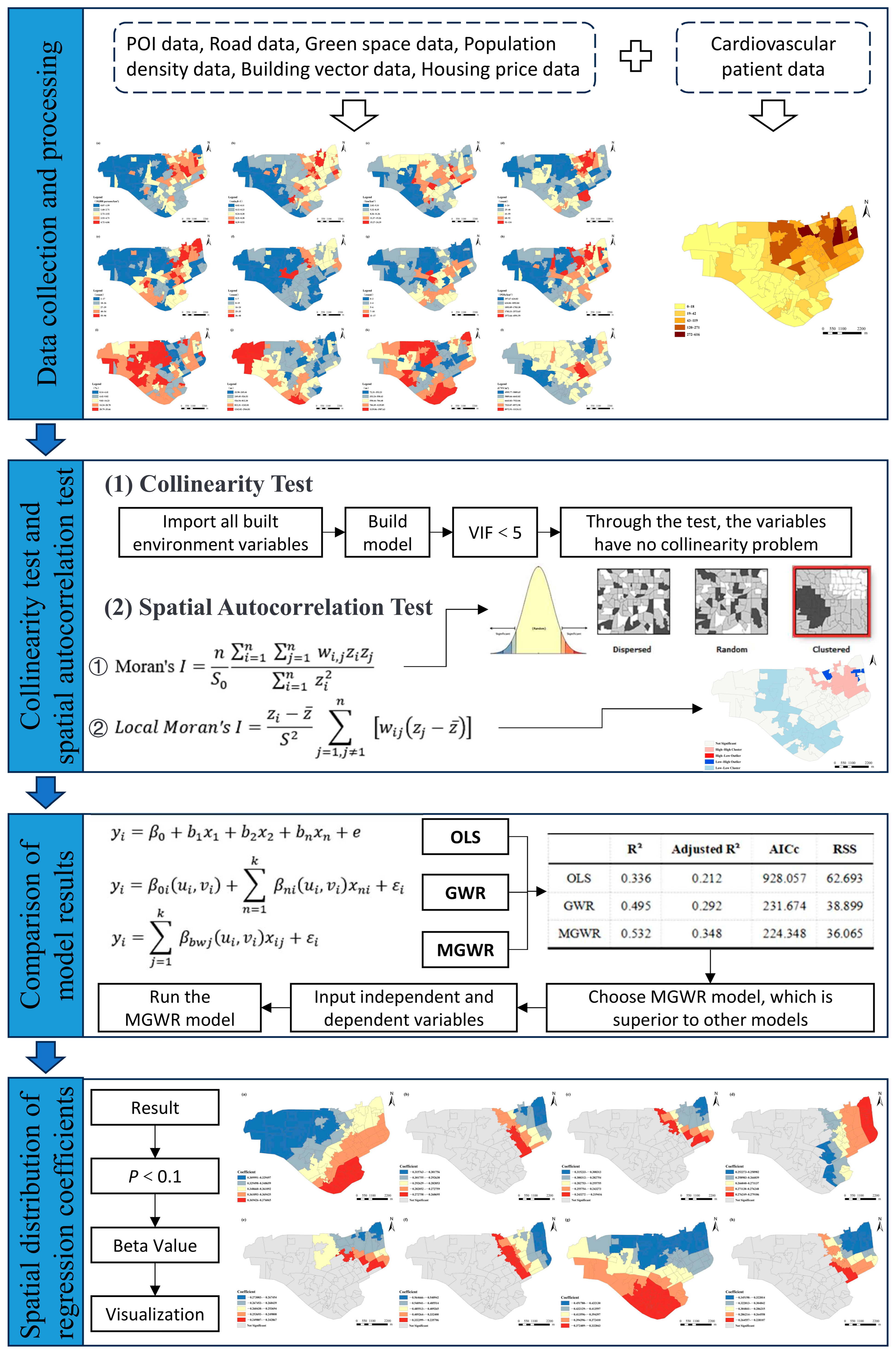
In this study, the MGWR model is applied to investigate the impact of built environment factors on cardiovascular health using hospital-based cardiovascular patient data. The research process consists of four main steps. First, multi-source built environment data and cardiovascular disease data are integrated to systematically construct a geospatial database and conduct data preprocessing. Second, variables with no multicollinearity (variance inflation factor, VIF < 5) are selected, and spatial autocorrelation tests are performed in ArcGIS to eliminate built environment variables that lack spatial correlation. Subsequently, OLS, GWR, and MGWR models are constructed, with GWR and MGWR models developed using MGWR 2.2 software provided by Arizona State University.
In the MGWR model, Adaptive Bisquare is adopted as the Spatial Kernel. It defines the bandwidth by the “number of nearest neighbors” rather than a fixed distance, which can automatically adjust the neighborhood size in the case of uneven distribution of communities. Meanwhile, the Bisquare function forces the weights to be set to 0 outside the specified neighborhood, effectively suppressing distant noise. The golden section is employed as the bandwidth searching method for this model. The golden section search continuously narrows the range where the optimal value exists, thereby finding the extremum. Additionally, the model’s optimization criterion is set to AICc. AICc builds upon AIC by incorporating a correction term for small sample sizes, providing a more accurate reflection of model complexity and fit, and avoiding model selection bias that may arise from small sample sizes. By comparing metrics such as R2, adjusted R2, Akaike Information Criterion (AICc), and residual sum of squares (RSS), the superiority of the MGWR model in capturing multi-scale spatial heterogeneity is verified, and the MGWR model is ultimately adopted. Finally, significant regression coefficients (p < 0.1) from the MGWR results are visualized using the ArcGIS platform to reveal the localized spatial gradient characteristics of the built environment’s influence on cardiovascular health. The research workflow is illustrated in Figure 2.

2.3.2. Spatial Autocorrelation Testing

This study adopts spatial autocorrelation analysis to investigate the spatial distribution characteristics of cardiovascular diseases and uncover their clustering patterns. Specifically, global spatial autocorrelation (Moran’s I) and local spatial autocorrelation (Local Moran’s I) are applied to assess the global and local spatial correlations of cardiovascular diseases, thereby identifying high-incidence, low-incidence, and outlier regions, and offering critical insights for subsequent attribution analysis. Moran’s I ranges between −1 and 1. A Moran’s I value greater than 0 indicates positive spatial correlation, with larger values representing stronger correlation; a value less than 0 indicates negative spatial correlation, with smaller values reflecting greater disparity; a Moran’s I of 0 suggests a random spatial distribution [54,55]. The global Moran’s I is calculated as:
Moran s   I = n S 0 i = 1 n   j = 1 n   w i , j z i z j i = 1 n   z i 2
where z i denotes the deviation of sample i from the mean, w i , j represents the spatial weight matrix, n is the total number of samples, and S 0 is the sum of all spatial weights.
S 0 is defined as:
S 0 = i = 1 n   j = 1 n   w i , j
where w i , j represents the spatial weight between i and j , and n denotes the total sample size.
Local spatial autocorrelation is employed to identify local clustering patterns within the data, elucidating the relationship between an observation at a specific location and those of its neighboring areas, thereby detecting local high-value or low-value clusters. The Local Moran’s I is defined as:
L o c a l   M o r a n s   I = z i z ¯ S 2 j = 1 , j 1 n   w i j z j z ¯
where z i is the value of the variable at location i , z ¯ is the mean of variable z , S 2 is the variance of z , and w i , j denotes the spatial weight between i and j .

2.3.3. Ordinary Least Squares (OLS)

OLS is a classical linear regression approach designed to establish the relationship between independent and dependent variables. This model assumes that the relationship remains constant across the study area, irrespective of spatial location, thereby neglecting spatial heterogeneity [56]. The OLS model is expressed as:
y i = β 0 + b 1 x 1 + b 2 x 2 + b n x n + e
where y i denotes the dependent variable, representing the number of cardiovascular cases in a community; β 0 is the intercept; b 1 , b 2 , …, b n represent the regression coefficients (slopes) for the independent variables x 1 , x 2 , …, x n ; and e is the residual term.

2.3.4. Geographically Weighted Regression (GWR)

GWR extends the OLS model by accounting for the spatial location of data, allowing parameter estimates to vary geographically [48,57]. The GWR model is expressed as:
y i = β 0 i u i , v i + n = 1 k   β n i u i , v i x n i + ε i
where y i denotes the number of cardiovascular disease cases in community i ; u i , v i represents the centroid coordinates of community i ; β 0 i u i , v i is the local intercept, and β n i u i , v i are the local coefficients for the nth independent variable; x n i is the value of the nth independent variable at location i ; and ε i denotes the random error term.

2.3.5. Multi-Scale Geographically Weighted Regression (MGWR)

GWR effectively captures the spatial non-stationarity in the relationship between response and explanatory variables; however, it applies a single fixed bandwidth for all explanatory variables. In contrast, MGWR permits each explanatory variable to operate at its optimized spatial scale, enabling a more precise characterization of spatial heterogeneity [49,58]. The model is expressed as:
y i = j = 1 k   β b w j u i , v i x i j + ε i
where y i denotes the dependent variable, representing the number of cases in community i ;
b w j is the bandwidth applied to the j th variable’s regression coefficient; β b w j u i , v i is the regression coefficient for the j th built environment variable in community i at bandwidth b w j ; x i j represents the j th built environment variable in community i ; and ε i denotes the error term.

3. Results

3.1. Spatial Distribution and Clustering Characteristics of Cardiovascular Patients

3.1.1. Spatial Distribution

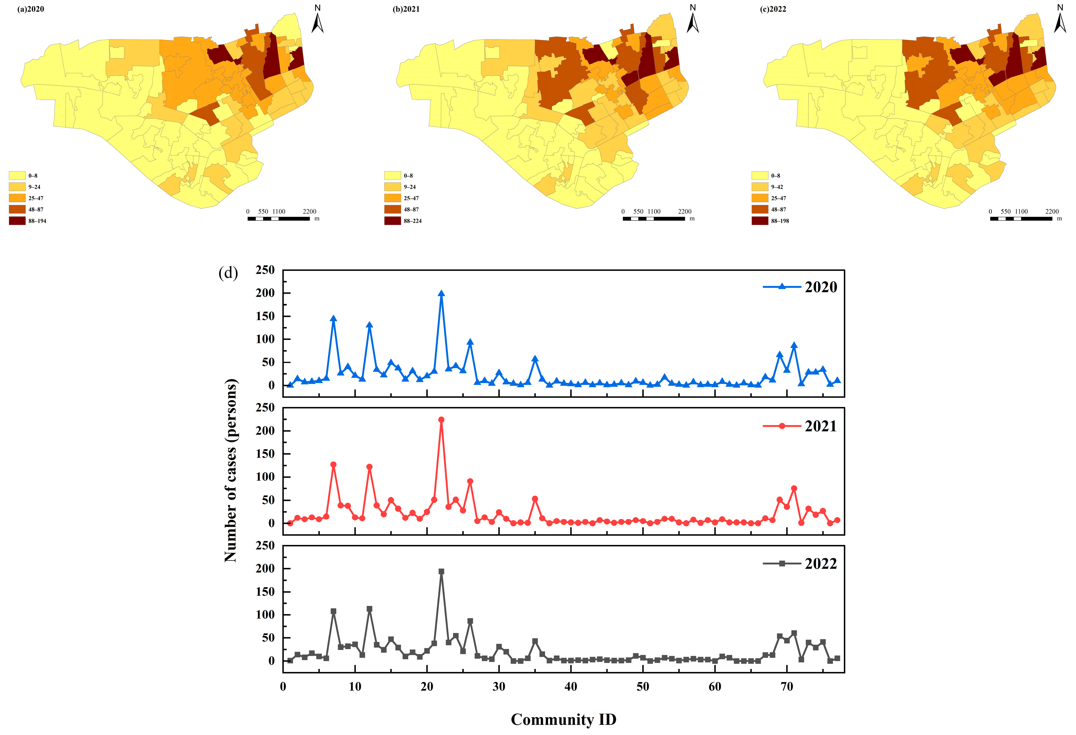
After cleaning the diagnostic data from Guangxi Nationalities Hospital, a total of 4770 cardiovascular patient cases were documented in the study area between 2020 and 2022. Specifically, there were 1547 cases in 2020, 1590 in 2021, and 1633 in 2022, demonstrating an overall upward trend, albeit with relatively modest year-on-year growth. The study area comprises 77 community committees. Based on the distribution maps of cardiovascular patient numbers from 2020 to 2022, the spatial distribution exhibits evident clustering, primarily concentrated in the eastern and northeastern sections of the area. Notably, clustering is observed in densely populated communities such as Mingxiu Second District, Youai North, Xiuhu, and Mingxiu North. These communities collectively account for 38.85% of total cases across the three years, with detailed spatial distribution characteristics illustrated in Figure 3.

3.1.2. Spatial Clustering Characteristics of Cardiovascular Patients at the Community Level

Supported by Geographic Information Systems (GIS), this study systematically analyzes the spatial clustering of cardiovascular patients across communities in the study area using global and local spatial autocorrelation analyses. Global spatial autocorrelation analysis is designed to reveal the overall spatial distribution patterns across the study area, while local spatial autocorrelation analysis further explores the spatial clustering characteristics within individual communities. Through local spatial autocorrelation analysis, the study identifies distinctive spatial patterns, such as high-value areas adjacent to low-value areas or vice versa, thereby uncovering potential environmental factors and the spatial variability underlying cardiovascular disease occurrences.
The global spatial autocorrelation analysis for the total number of cardiovascular cases in communities within the express ring road of Xixiangtang District, Nanning, yields a Moran’s I value of 0.28, significantly higher than the expected value of −0.013, indicating that cardiovascular case numbers exhibit spatial correlation across communities in the study area from 2020 to 2022. Additionally, the Z-score is 4.98 and the p-value is 0.000001, satisfying the 99% confidence level for statistical significance, indicating a significant clustering pattern of cardiovascular disease cases within communities in the study area.
In the local spatial autocorrelation analysis, the General G statistic for the total cardiovascular case count across communities is 0.000275, exceeding the expected value of 0.000131, accompanied by a Z-score of 4.931453 and a p-value of 0.000001, indicating a significantly high clustering pattern in the distribution of cardiovascular cases across communities. The results suggest a pronounced spatial clustering effect of cardiovascular cases within the study area, with high-case communities tending to cluster together, demonstrating a concentration of cardiovascular diseases in specific regions. Specifically, the spatial distribution of cardiovascular cases among communities in the study area demonstrates significant spatial inequality, characterized by four spatial patterns: high–high clusters (HH), low–low clusters (LL), high–low clusters (HL), and low–high clusters (LH) (Figure 4). HH clusters are primarily concentrated in areas such as Xiuhu Community and Mingxiu Community, suggesting the presence of shared risk factors that contribute to the high prevalence of cardiovascular diseases in these regions. LL clusters are predominantly located in areas such as Daxue East Road Community and Keyuan Avenue Community, indicating the presence of protective factors that may lower the risk of cardiovascular diseases in these regions. The number of HL and LH clustered communities is relatively small, but these areas still merit attention for investigating the potential impacts of adjacency between high- and low-incidence communities.

3.2. Spatial Distribution Characteristics of the Built Environment

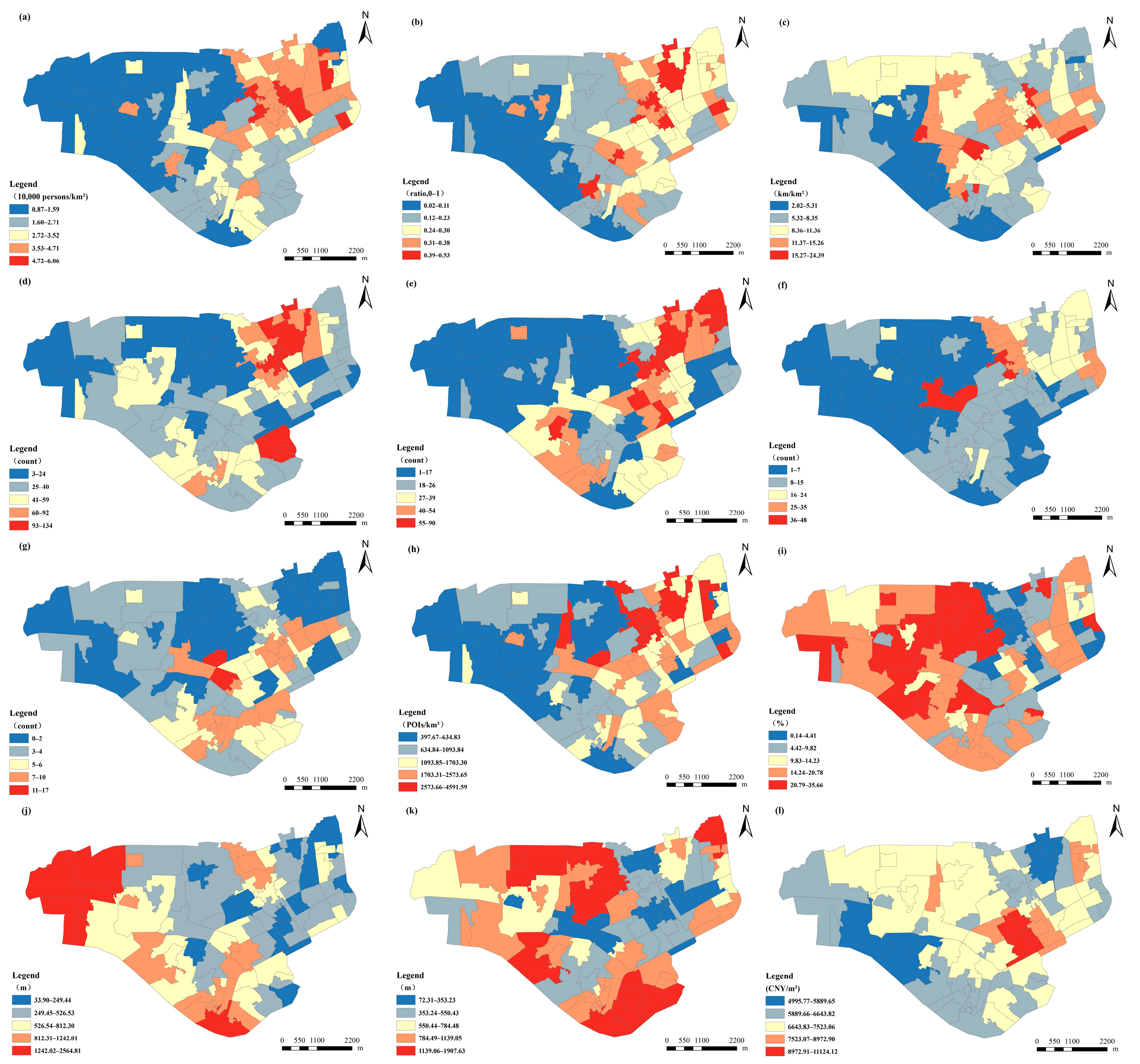
Moran’s I is employed as the metric to assess the spatial correlation of each selected independent variable, and the results indicate that for all independent variables, Moran’s I values are positive, Z-scores exceed 1.96, and p-values are below 0.05, suggesting that spatial autocorrelation exists at the 95% confidence level, indicating that the spatial distribution of the independent variables exhibits clustering characteristics. The spatial distribution of the built environment is visualized in Figure 5.
The spatial distribution of built environment elements within the study area exhibits marked unevenness. Eastern communities, including Xiuling South, Xinxiu, Mingxiu South, and Mingxiu North, are densely populated, largely due to convenient transportation, affordable rental housing, and abundant employment opportunities in these areas. Wanxiu Village, the largest urban village in Xixiangtang District, exhibits high population density, which promotes the clustering of both healthy and unhealthy food outlets. Additionally, recreational and sports facilities, bus and metro stations, and facility POI density exhibit high values around Guangxi University and Wanxiu Village, reflecting population concentration and diversified service demands. By contrast, the western and southwestern areas, characterized by remoteness, lower economic levels, and underdeveloped infrastructure, are sparsely populated with limited access to facilities and services. In terms of community green space ratio, central and western communities such as Guangxi University and Keyuan Avenue demonstrate higher green coverage, highlighting their favorable positioning within urban planning. In contrast, the area surrounding Wanxiu Village has limited green space due to high building density. Residents in central and eastern communities are located closer to the nearest parks and squares, whereas those in the west and south are farther away, indicating disparities in infrastructure distribution across these areas. Several communities in the southern and northwestern parts of the study area are farther from metro stations, largely due to their distance from the city center and limited metro coverage. The average housing prices are higher in areas surrounding Nantie Community, attributed to its advantageous location, convenient transportation, favorable environment, and rich educational resources.

3.3. Model Comparison Results

Based on the 12 variables that passed the multicollinearity and spatial autocorrelation tests, OLS, GWR, and MGWR models were constructed. As shown in Table 3, among the three models, the MGWR model exhibits the best goodness-of-fit, with the highest R2 value, suggesting the strongest explanatory capacity and greater accuracy in capturing the relationship between the dependent and independent variables. The adjusted R2 further demonstrates that the MGWR model maintains its advantage after accounting for degrees of freedom, with improvements of 0.136 and 0.056 over the OLS and GWR models, respectively. Additionally, a lower AICc value suggests a higher model quality. The MGWR model’s AICc value is significantly lower than those of the GWR and OLS models, reduced by 703.709 and 7.326, respectively, suggesting that the model achieves a better fit while effectively balancing model complexity, leading to superior predictive accuracy. Finally, the MGWR model yields the smallest RSS, indicating minimal differences between the predicted and observed values. Further conducting spatial autocorrelation tests on the residuals of the three models, we obtained the following results: The Moran’s I value for the OLS model was −0.023, for the GWR model it was −0.066, and for the MGWR model it was −0.058. This indicates that the residuals of all three models do not show statistically significant spatial autocorrelation.
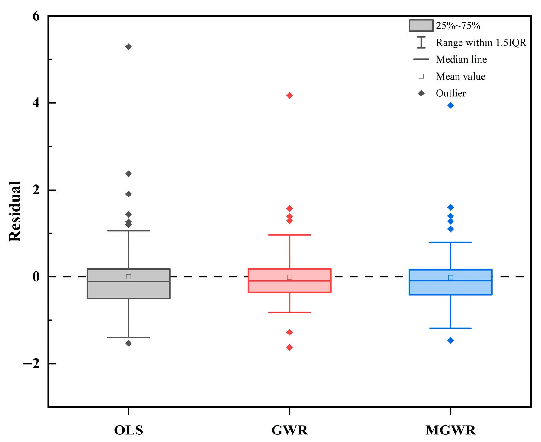
Subsequently, boxplots (Figure 6) were employed to compare the residuals of the OLS, GWR, and MGWR models. The results reveal that the median residual for OLS is −0.104, for GWR is −0.090, and for MGWR is −0.087. The median line in the MGWR boxplot lies closer to 0, with the smallest interquartile range and the fewest outliers, indicating a more concentrated residual distribution, lower residual values, and superior model fit.
In conclusion, although the residuals of the OLS model perform better in terms of spatial randomness, the MGWR model demonstrates superior performance in terms of goodness of fit, explanatory power, prediction accuracy, and spatial autocorrelation of residuals. This finding confirms the superiority of the MGWR model in spatial heterogeneity analysis, enabling it to effectively capture the spatial heterogeneity in the data while maintaining low spatial autocorrelation of residuals, thereby confirming the superiority of the MGWR model in the analysis.
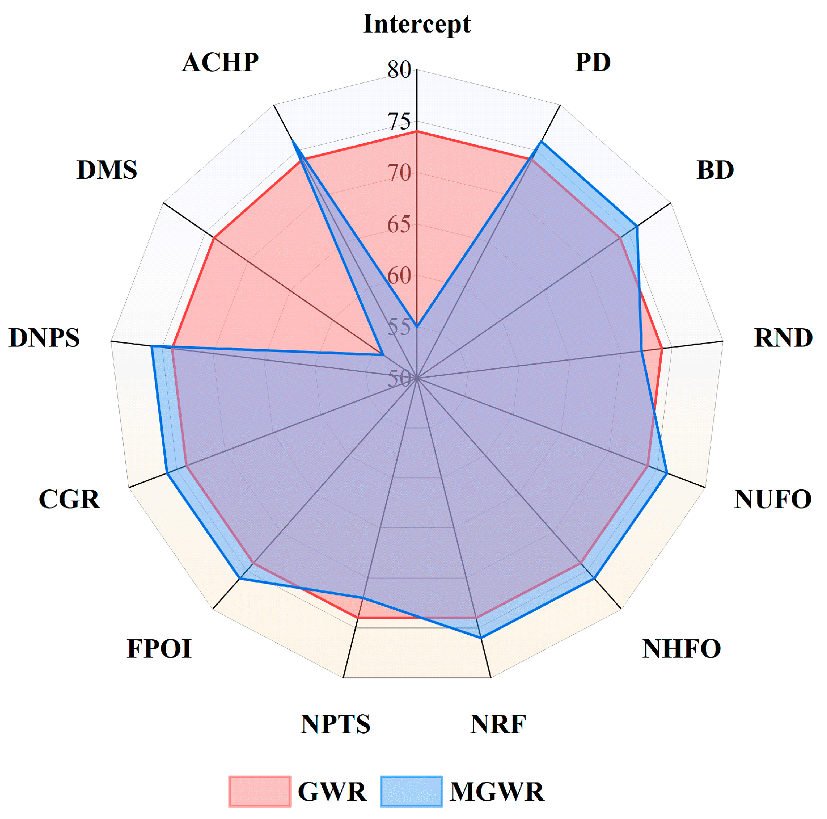
In terms of bandwidth configuration, the GWR model assumes that all explanatory variables share a consistent spatial scale of influence, with a bandwidth of 74. In contrast, the MGWR model relaxes this constraint by allowing variables to exhibit heterogeneous spatial effects, with bandwidths ranging between 54 and 76 (Table 4). The results indicate that the influence of built environment elements on cardiovascular health not only varies in intensity but also demonstrates significant spatial non-stationarity (Figure 7). In summary, the MGWR model achieves a superior balance among explanatory power, model complexity, and predictive performance. It more effectively captures the localized characteristics of variables, thereby more accurately revealing the complex relationship between the built environment and cardiovascular health.

3.4. Spatial Heterogeneity Analysis of Influencing Factors

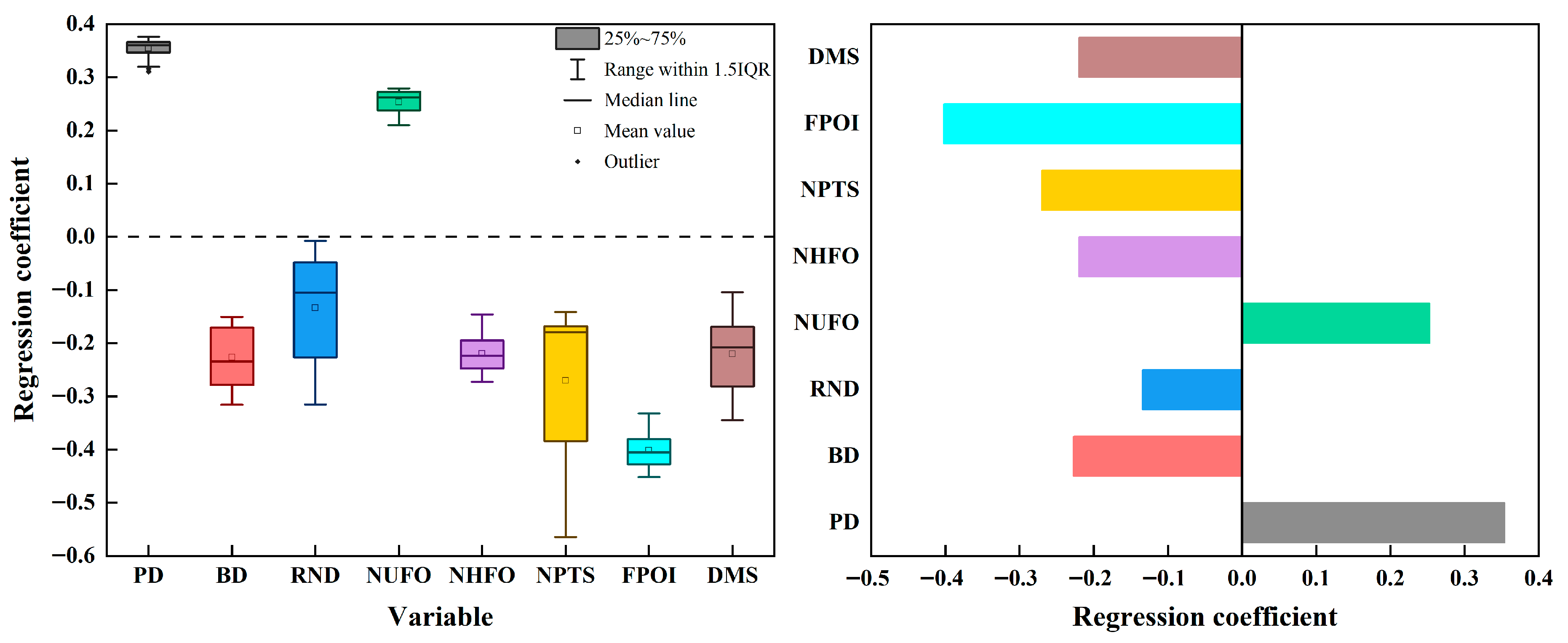
Table 5 summarizes the regression coefficient statistics for built environment variables in the MGWR model. The model identifies eight variables, population density, building density, road network density, number of unhealthy food outlets, number of healthy food outlets, number of bus and metro stations, facility POI density, and distance to metro stations, as exhibiting significant spatial effects at the 90% confidence level, confirming their heterogeneous influence on cardiovascular case numbers across the study area. The remaining variables (number of recreational facilities, community green space ratio, distance to the nearest park or square, and average community housing prices) did not achieve statistical significance. The distribution characteristics of these regression coefficients for the significant variables are further illustrated by the boxplots in Figure 8.
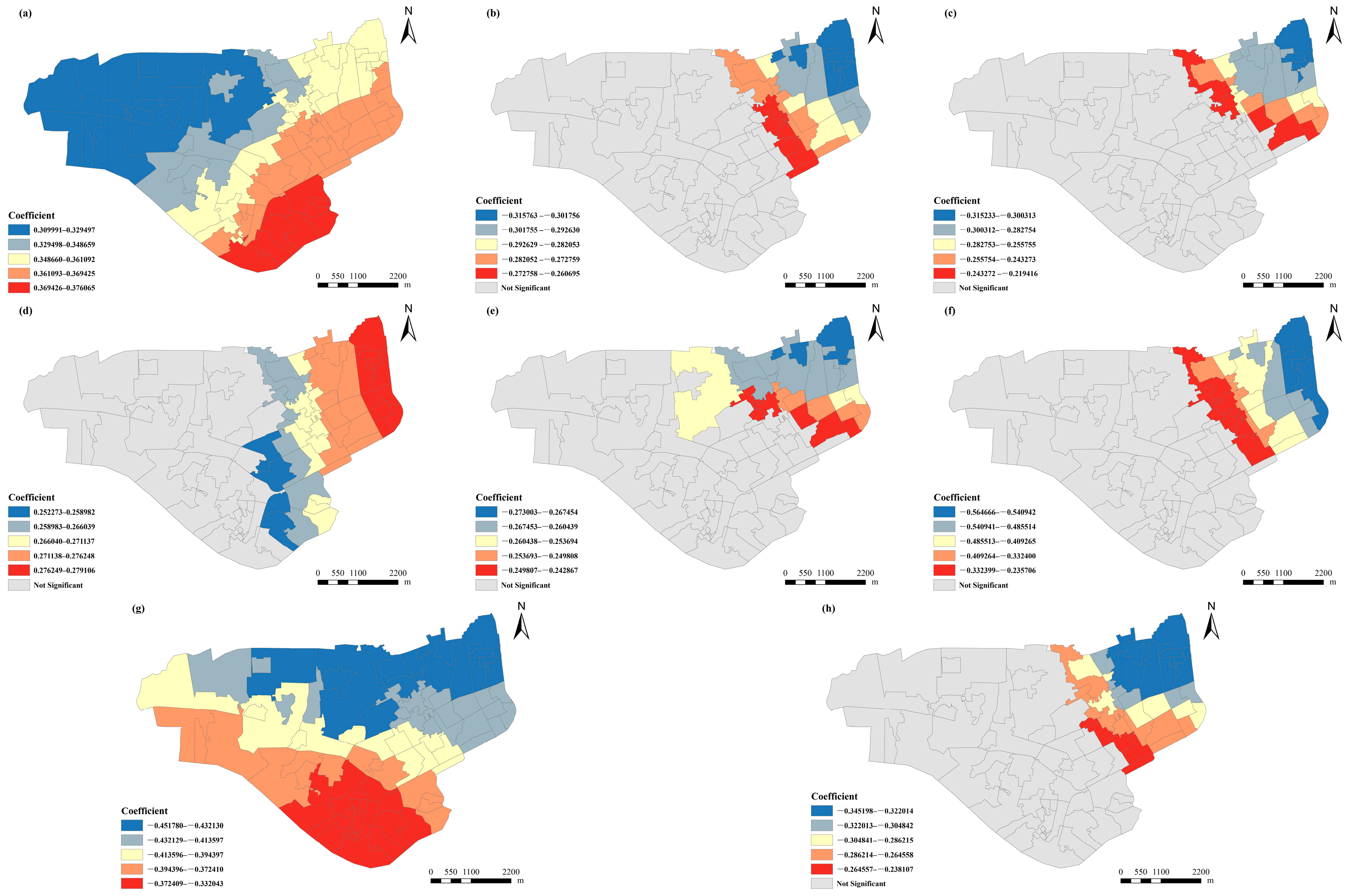
The spatial distribution of regression coefficients for significant variables was visualized using ArcGIS (Figure 9). Based on the scale and stability of their spatial effects, the significant variables can be categorized into three types:
The first category consists of variables with global-scale and homogeneous effects. Population density and facility POI density are not only universally significant across all 77 communities but also exhibit remarkable spatial consistency in the direction of their effects. Population density is a stable risk factor (Mean = 0.354), while facility POI density is a potent and stable protective factor (Mean = −0.402). Notably, while their effect directions are consistent globally, the strength of these effects shows substantial local variation. Population density’s risk effect reaches its peak in older urban neighborhoods such as Bianyang, Xinyangxia, and Beidanan within Xinyang Street, while demonstrating its weakest effects in newer developed areas including High-tech Industrial Park, Keyuan Avenue, and Jiangdong Community in Xinxu Street. Conversely, facility POI density’s protective effect shows precisely the opposite spatial intensity pattern. Its protective strength is weakest in older communities such as Nanji, Longteng, and Yongning in Xinyang Street, while reaching its maximum strength in neighborhoods including Beihu East, Xiuxiang, and Xiuhu within Beihu and Hengyang Streets. This creates a critical “double disadvantage” pattern in aging urban cores where the strongest population risk coincides with the weakest POI protection, while newly developed areas benefit from both diminished risk factors and enhanced protective environments. This high degree of spatial uniformity in effect direction strongly aligns with their large bandwidth (Bandwidth = 76) in the MGWR model, indicating that their influences operate at a global scale while still exhibiting important local variations in effect magnitude. The number of unhealthy food outlets exhibits high spatial stability as a widespread risk factor (Mean = 0.253; Std. = 0.022), with exclusively positive coefficients confirming its consistent risk effect across the study area. While demonstrating overall spatial stability, its effect intensity shows localized variations, with coefficient peaks primarily distributed in Beihu Street communities such as Beihu East and Mingxiu East, while the lowest values are concentrated in certain communities of Xixiangtang and Xinyang Streets, including Beida North Road, Shenyang Road, and Bianyangxia. This pattern suggests that although unhealthy food outlets function as a universal risk factor, their health impacts may be particularly pronounced in specific urban contexts where environmental or socioeconomic factors potentially amplify their detrimental effects.
The second category comprises variables with strongly localized and heterogeneous effects. The influence of distance to metro stations demonstrates pronounced spatial non-stationarity. It has the smallest bandwidth (54), meaning the model estimates its effect at a highly localized scale. This is directly reflected in its regression coefficients, which have a relatively large standard deviation (0.069) and a wide IQR range. A particularly critical finding is that its mean coefficient is significantly negative (−0.22), and all significant sample coefficients are negative. This suggests that, within the context of this study, greater distance from metro stations is associated with a lower risk of cardiovascular diseases. Spatially, the lowest absolute coefficient values are consistently located in Hengyang Street communities such as Zhonghua Middle Road, Hengyang South, and Xinxiu, while the highest absolute values are primarily distributed in certain communities of Beihu Street and Zaojiao Village community in Anning Street.
The third category includes variables with context-dependent effects and moderate spatial variability. These include building density, road network density, number of healthy food outlets, and number of public transport stations. Although they generally show protective effects (median coefficients are negative), their significance rates are relatively low (28.57–37.66%), and they have considerable standard deviations, with number of public transport stations exhibiting the largest coefficient fluctuation range (Range = 0.424). This indicates that they are not universal protective factors. The realization of their health benefits is highly dependent on unobserved local contexts (such as community-built environment quality, residents’ socioeconomic composition, or lifestyle patterns) and their protective effects are fully manifested only in communities with suitable conditions. Notably, spatial analysis reveals that the strongest protective effects (highest absolute coefficients) for these variables are concentrated in specific areas: building density peaks in Beihu Middle, Xiuxiang Road, and Chengchun communities; road network density shows maximum effects in Zaojiao Village and Beihu East; healthy food outlets exhibit the strongest protection in Xiuxiang Road and Chengchun communities. Conversely, the weakest effects are consistently found in Hengyang Street communities and the Guangxi University area. This stark spatial differentiation further underscores the critical importance of local context in determining these variables’ health impacts.

4. Discussion

4.1. Key Findings

This study aimed to investigate the spatial effects of the built environment on cardiovascular health and employed the MGWR model to analyze the multiscale relationship between built environment factors and cardiovascular diseases. Global and local spatial autocorrelation analyses revealed that the number of cardiovascular cases in communities within the study area exhibited significant spatial autocorrelation, where communities with high (or low) case numbers tended to cluster in adjacent areas, demonstrating clear spatial clustering patterns. In this study, the MGWR model increased the adjusted R2 by 0.136 and 0.056 compared to the OLS and GWR models, respectively, and reduced the AICc values by 703.709 and 7.326, respectively, indicating that the MGWR model more effectively captures the multiscale spatial heterogeneity between the built environment and cardiovascular case numbers in communities. By identifying three categories of variables operating at distinct spatial scales, the research demonstrates that the impact of environmental factors on health not only follows global patterns but, more importantly, exhibits rich local characteristics, which hold significant implications for understanding urban health geography patterns.
First, both population density and facility POI density demonstrated global and high-intensity influence characteristics in the MGWR model. Specifically, population density showed a significant positive correlation with the number of community cardiovascular cases. Existing research clearly indicates that residents living in high-population-density areas face a greater likelihood of increased risk of cardiovascular diseases and other non-communicable diseases [59], a conclusion further validated in this study. Research by Chandrabose et al. also suggests that urban population intensification may increase the risk of cardiovascular diseases by affecting physiological indicators such as blood lipids and blood pressure [60]. Areas with high population density tend to face greater health burdens. The underlying mechanism may stem from the combined effects of traffic pollution [61], exposure to airborne particulate matter [62] (e.g., NO2, particulate concentration), and socioeconomic pressures [63,64] within the built environment, thereby impacting residents’ cardiovascular health. In Xixiangtang, old urban areas (such as Xinyang Street) experience amplified cardiovascular health risks due to the combination of outdated infrastructure and high population density, leading to environmental pressures such as traffic pollution and poor ventilation. In contrast, emerging areas (such as the High-tech Zone) have effectively mitigated the negative effects of density through high-quality planning.
However, in sharp contrast to the risk effect of population density, facility POI density exhibits a global protective effect of equivalent strength but in the opposite direction. POI data can more objectively reflect the accessibility of public service facilities. High facility POI density improves daily convenience and optimizes residents’ activity ranges [65], thereby reducing reliance on transportation, promoting walking and other physical activities [66], ultimately delivering widespread cardiovascular health benefits to the community. In emerging communities such as the High-tech Zone and Xinxu Street, high facility POI density manifests as an organic combination of commercial complexes, scientific research service institutions, and parks, significantly promoting health benefits. In contrast, in old urban areas like Xinyang Street, traditional scattered stores and low-end markets, although constituting quantitative POI density, fail to effectively translate into health protection effects. This finding emphasizes that in modern urban planning, the critical regulatory role of urban planning on health outcomes should be fully recognized [67]. There is a need for coordinated regulation of population density and facility density, optimized spatial resource allocation to maximize health benefits.
Furthermore, the number of unhealthy food outlets was also identified as a highly stable global risk factor. Its regression coefficients were positive in all statistically significant communities, with minimal standard deviation, confirming its role as a widespread and consistent negative health influence across the study area. A higher density of unhealthy food outlets implies easier resident access to foods high in salt, sugar, and fat. This unhealthy “food environment” directly increases the probability of residents developing cardiovascular disease risk factors, such as obesity and hypertension, by promoting unhealthy dietary behaviors [33]. Related studies have shown a significant association between the prevalence of unhealthy food outlets and cardiovascular health outcomes [68,69]. Moreover, high consumption of unhealthy foods among residents is linked to an increased risk of cardiovascular diseases [70].
The impact of distance to metro stations exhibits a highly localized and complex pattern. Across all statistically significant samples, the regression coefficients for this variable were consistently negative, suggesting that greater distance from metro stations is overall associated with a lower risk of cardiovascular diseases in this study. This finding aligns with results reported by Zhang et al., who observed a significant negative correlation between proximity to the nearest transit stop and physical health among older adults [71]. The underlying mechanisms for this phenomenon may be twofold. On the one hand, behavioral pathways may play a role: although convenient transportation reduces commute times, it may also limit physical activity, thereby increasing the risk of overweight and obesity and adversely affecting residents’ health [72]. On the other hand, environmental exposure is another plausible pathway: while metro commuting alleviates urban traffic congestion, the interior of subway cars constitutes a known microenvironment for exposure to air pollutants, such as PM2.5 [73]. Longer commute times imply prolonged exposure, which can exacerbate health burdens. Moreover, increased concentration of PM2.5, a key component of such pollutants, has been confirmed to directly and negatively affect cardiovascular health [74]. Therefore, the health benefit observed in this study associated with “increased distance from metro stations” may result from a comprehensive reduction in exposure to metro-related commuting behaviors and their associated environmental pollutants.
The study further confirms that building density, road network density and public transport stations generally demonstrate potential protective tendencies (all regression coefficients are negative). These elements collectively characterize areas with higher functional mix and enhanced walkability, which help residents maintain active lifestyles and thereby promote cardiovascular health. This finding is consistent with previous studies indicating that the walkability of the built environment is negatively correlated with cardiovascular disease risk factors; residing in highly walkable communities helps reduce the prevalence of these risk factors and thus improves cardiovascular health levels [75,76,77,78,79,80]. Similarly, the number of healthy food outlets within communities is negatively associated with cardiovascular disease incidence among residents. Li et al.’s study using APCAPS data in India linked higher vegetable and fruit vendor density to lower blood pressure, and higher processed food and takeout density to higher blood pressure and obesity [81]. This discovery holds significant reference value for other developing countries, highlighting the importance of the food environment as a factor influencing cardiovascular health.
However, an important contribution of this study lies in revealing that the protective effects of these elements are not automatically realized but largely depend on their deep integration with the local context. For example, the protective effects of building density and public transport stations are more pronounced in communities with well-developed supporting facilities and favorable socioeconomic conditions, such as Beihu, Xiuxiang Road, and Chengchun. In contrast, in functionally homogeneous or socially underserved areas (e.g., around Guangxi University), the same facilities fail to demonstrate significant health benefits. This indicates that high density and abundant facilities can translate their potential protective tendencies into tangible health benefits only when combined with a high-quality local environment that supports active lifestyles [82].
Finally, the number of recreational facilities, community green space ratio, and distance to the nearest park or square did not show significant effects on cardiovascular health. This lack of significance might be attributed to various factors related to data collection, such as the distribution, quality, accessibility, and utilization rates of these facilities. The research by Paquet et al. also confirmed that larger, greener, and more active public open spaces are associated with better cardiovascular and metabolic health, but the quantity and proportion of public open spaces are not related to cardiovascular and metabolic health [83]. Despite these non-significant findings, these factors may still play a role in influencing residents’ health behaviors and outcomes in actual built environments. For instance, when residents use public transportation, they may have more access to green spaces and recreational facilities. These environments may have positive effects on health by providing relaxation and improving air quality, among other things. Previous research indicates that the proximity, connectivity, and accessibility of public facilities significantly influence residents’ physical activity and health outcomes [84]. Meanwhile, the health benefits of green spaces are contingent upon residents’ engagement, with accessibility, visibility, and usability identified as critical factors [85,86]. Furthermore, average community housing prices also showed no significant association, possibly due to the complex relationship between housing prices and health, which exhibits notable heterogeneity across different outcomes and populations [87,88]. As Sims et al. pointed out, the impact of housing on cardiovascular health is achieved through various means, including stability, quality, affordability, and the surrounding environment [89]. This indicates that merely relying on average housing prices may not fully reflect the situation in these aspects. Thus, future studies should integrate granular measures of housing quality and accessibility to better elucidate its health effects.

4.2. Policy Implications

This study integrates a multi-level socio-ecological framework with spatial econometric models to empirically validate the spatial heterogeneity in the health impacts of the built environment, thereby advancing the understanding of environment-health relationships in health geography. In summary, to enhance cardiovascular health among community residents, communities should optimize walking environments by adding sidewalks and barrier-free facilities, promote mixed-use community designs, enhance walkability, and reduce dependence on motorized transport. For communities with a high density of unhealthy food outlets, governments should limit fast-food outlet density and introduce fresh food supermarkets or farmers’ markets, thereby improving access to healthy foods and enhancing residents’ dietary environments and structures. These measures should be given priority in the short term, as they can rapidly improve the health environment and directly influence residents’ health behaviors, especially in communities where the incidence of cardiovascular diseases is on the rise. In the coming years, urban planners should prioritize developing more public spaces and fitness facilities in densely populated and highly built-up com-munities to alleviate environmental stress and provide convenient opportunities for physical activity. Meanwhile, public facility layouts should be optimized to ensure proximity, connectivity, and accessibility, while enhancing facility quality and expanding diverse recreational and exercise options to increase utilization among residents. Regarding the impacts of metro station distance and the number of bus stops, urban planning should focus on enhancing transportation accessibility, particularly by adding bus routes or micro-circulation shuttles in underserved communities to eliminate “last-mile” commuting barriers. In the long term, future metro planning should prioritize underserved areas, optimizing route designs and shortening commuting times, while enhancing air quality monitoring and improvements within train carriages to reduce health burdens.

4.3. Limitations and Future Research Directions

In this study, the MGWR model demonstrated superior goodness-of-fit relative to the OLS and GWR models, owing to its capacity to effectively handle spatial heterogeneity and multiscale relationships. However, it is essential to acknowledge that the MGWR model is based on linear relationships, and it does not fully account for potential nonlinear associations between the built environment and health outcomes. This limitation is particularly relevant in understanding complex environmental-health interactions, as some relationships may not be captured using linear models. Moreover, MGWR’s effectiveness is dependent on the data quality, and in areas with sparse data or high variability, model performance may be compromised. Secondly, as a cross-sectional study, this research cannot establish causal relationships [17]. The reliance on cross-sectional data introduces the potential for reverse causality and makes it difficult to infer long-term impacts of built environment factors on cardiovascular health. The short time span of the data used in this study also limits the ability to capture dynamic changes over time, which are crucial to understanding the evolving relationship between the built environment and health outcomes. Furthermore, the model’s focus on certain built environment variables means that other potentially influential factors (e.g., social determinants of health, personal behaviors) have been omitted. While we controlled for population density, other confounders such as smoking, alcohol consumption, and occupation, which are known to influence cardiovascular health, were not included. This omission could introduce bias into the model, affecting the overall accuracy of the findings. The data for this study originated from a single public hospital, which may not accurately reflect the treatment patterns of other healthcare facilities, including private hospitals. This limitation in data representativeness may impact the generalizability of the results. The reliance on data from a single hospital may skew the results due to underreporting from patients seeking care outside of this institution. This could result in biases due to patient preferences and healthcare-seeking behaviors that are not captured in the study. Although population density was controlled in our model, the case numbers were neither standardized nor log-transformed, potentially affecting result reliability due to scale effects. The lack of standardization or transformation could lead to misleading conclusions about the spatial distribution of health outcomes. In particular, scale effects may exacerbate the influence of certain variables, especially in regions with extreme values. Furthermore, the study was conducted in a single urban district, which restricts the generalizability of the findings. The generalizability of these findings is limited to urban contexts similar to that of Xixiangtang District in Nanning. Therefore, caution should be exercised when extrapolating the results to rural settings or cities in other countries. Furthermore, as the analysis did not stratify outcomes by age, gender, or specific types of cardiovascular diseases, the conclusions may not be fully applicable across different population subgroups.
In light of these limitations, future research should focus on models capable of capturing nonlinear relationships, such as random forests or other machine learning algorithms, which can better account for complex interactions between built environment factors and health outcomes. Additionally, methods such as kernel density smoothing or weighted regression could be utilized to address data imbalance and improve the model’s robustness. Longitudinal or intervention-based study designs are recommended to explore causal mechanisms and improve the accuracy of the findings. To enhance the generalizability of the research findings, future studies should expand the time span of the data, update the data annually, add more diverse built environment variables (such as air pollution, noise, and heat exposure), incorporate personal and social factors, and broaden the data sources. The inclusion of more granular spatial data and qualitative research approaches would also help address the issue of confounding factors and provide a more comprehensive understanding of how the built environment affects cardiovascular health.

5. Conclusions

This study focused on communities located within the first ring road of Xixiangtang District, Nanning, and applied the MGWR model to uncover differences in the spatial scales at which various built environment factors exert influence, thereby highlighting the spatial heterogeneity in the effects of built environment factors on cardiovascular health, offering new empirical evidence on the relationship between the built environment and cardiovascular health in urban environments of developing countries. The findings suggest that the MGWR model outperforms both the OLS and GWR models in terms of goodness-of-fit and explanatory power, enabling more precise capture of the complex associations between the built environment and cardiovascular diseases and identifying the spatial scales at which different environmental characteristics operate.
The main findings of this study include population density and the number of unhealthy food outlets are positively associated with cardiovascular cases, indicating that communities with higher population density or more unhealthy food outlets may face higher cardiovascular health risks, whereas building density, road network density, the number of healthy food outlets, public transport stations, facility POI density, and distance to metro stations are negatively associated with cardiovascular cases, suggesting that these factors provide protective effects. These relationships exhibit spatial heterogeneity, with varying intensities and directions across different communities. Thus, urban planning and public health policies should be tailored to each community’s specific conditions, adopting context-specific strategies. For example, communities with high population density or a high number of unhealthy food outlets should limit fast-food availability and increase access to healthy food outlets; in communities with inadequate public transportation, efforts should focus on increasing bus routes or improving metro station accessibility. Additionally, improving air quality within metro stations, such as enhancing ventilation systems and reducing air pollution exposure, can help mitigate health risks related to cardiovascular diseases. By implementing these targeted policies, urban planners can effectively improve residents’ cardiovascular health.
However, this study also has limitations, particularly regarding the exclusion of other potential health determinants such as individual behaviors, socioeconomic factors, and healthcare resource distribution. Moreover, as this study was limited to the Xixiangtang District of Nanning, the applicability of the findings to other cities or regions, especially those at different stages of urban development, needs further validation. Future studies should incorporate more social, economic, and behavioral data to more comprehensively assess the factors influencing cardiovascular diseases, providing broader insights for health policy development.

Author Contributions

Conceptualization, Shuguang Deng and Shuyan Zhu; methodology, Shuyan Zhu; software, Shuyan Zhu; vali-dation, Shuguang Deng and Shuyan Zhu; formal analysis, Shuyan Zhu; investigation, Shuguang Deng and Shuyan Zhu; resources, Shuguang Deng and Xueying Chen; data curation, Shuguang Deng, Shuyan Zhu, Xueying Chen, Jinlong Liang and Rui Zheng; writing—original draft preparation, Shuyan Zhu; writing—review and editing, Shuguang Deng and Shuyan Zhu; visualization, Shuyan Zhu; supervision, Shuguang Deng and Xueying Chen; project administration, Shuguang Deng and Xueying Chen; funding acquisition, Shuguang Deng and Xueying Chen All authors have read and agreed to the published version of the manuscript.

Funding

This research was supported by the Guangxi Science and Technology Program for Technology Base and Fostering Talents, “Quality of Life: Time Allocation and Travel Behaviors of Urban Residents across Age Groups” (Grant No. Guike AD23026234), and the Guangxi Higher Education Institutions Young and Middle-aged Teachers’ Research Capacity Improvement Project, “Subjective Well-being of Rural and Urban Elderly: from the perspective of Public Facilities and Service Equalization” (Grant No. 2023KY0397).

Data Availability Statement

The raw data supporting the conclusions of this article will be made available by the authors on request.

Acknowledgments

Thanks to the anonymous reviewers and editors for their comments and insights to improve this paper.

Conflicts of Interest

The authors declare no conflicts of interest.

Abbreviations

The following abbreviations are used in this manuscript:
CVDCardiovascular Disease
GBDGlobal Burden of Disease
WHOWorld Health Organization
OLSOrdinary least squares
GWRGeographically weighted regression
MGWRMulti-scale geographically weighted regression
POIPoints of interest
VIFVariance inflation factor
NCCNumber of Cardiovascular Cases
PDPopulation Density
BDBuilding Density
RNDRoad Network Density
LUMELand Use Mix Entropy
NUFONumber of Unhealthy Food Outlets
NHFONumber of Healthy Food Outlets
NRFNumber of Recreational Facilities
NPTSNumber of Public Transport Stations
FPOIFacility POI Density
CGRCommunity Green Space Ratio
DNPSDistance to Nearest Park or Square
DBSDistance to Nearest Bus Stop
DMSDistance to Nearest Metro Station
ACHPAverage Community Housing Price
RSSResidual sum of squares
GISGeographic Information Systems
HHhigh–high clusters
LLlow–low clusters
HLhigh–low clusters
LHlow–high clusters

References

  1. Roth, G.A.; Mensah, G.A.; Johnson, C.O.; Addolorato, G.; Ammirati, E.; Baddour, L.M.; Barengo, N.C.; Beaton, A.Z.; Benjamin, E.J.; Benziger, C.P.; et al. Global Burden of Cardiovascular Diseases and Risk Factors, 1990–2019: Update from the GBD 2019 study. J. Am. Coll. Cardiol. 2020, 76, 2982–3021. [Google Scholar] [CrossRef] [PubMed]
  2. Non-Communicable Disease. Available online: https://www.who.int/zh/news-room/fact-sheets/detail/noncommunicable-diseases (accessed on 27 November 2024).
  3. Wang, Y.; Wang, J. Modelling and prediction of global non-communicable diseases. BMC Public Health 2020, 20, 822. [Google Scholar] [CrossRef] [PubMed]
  4. Lai, K.Y.; Webster, C.; Gallacher, J.E.J.; Sarkar, C. Associations of Urban Built Environment with Cardiovascular Risks and Mortality: A Systematic Review. J. Urban Health 2023, 100, 745–787. [Google Scholar] [CrossRef]
  5. Bhatnagar, A. Environmental Determinants of Cardiovascular Disease. Circ. Res. 2017, 121, 162–180. [Google Scholar] [CrossRef]
  6. Pinter-Wollman, N.; Jelić, A.; Wells, N.M. The impact of the built environment on health behaviours and disease transmission in social systems. Philos. Trans. R. Soc. B Biol. Sci. 2018, 373, 20170245. [Google Scholar] [CrossRef]
  7. Malambo, P.; Kengne, A.P.; De Villiers, A.; Lambert, E.V.; Puoane, T. Built Environment, Selected Risk Factors and Major Cardiovascular Disease Outcomes: A Systematic Review. PLoS ONE 2016, 11, e0166846. [Google Scholar] [CrossRef]
  8. Cardiovascular Disease. Available online: https://www.who.int/zh/news-room/fact-sheets/detail/cardiovascular-diseases-(cvds) (accessed on 27 November 2024).
  9. Dummer, T.J. Health geography: Supporting public health policy and planning. CMAJ Can. Med. Assoc. J. Medicale Can. 2008, 178, 1177–1180. [Google Scholar] [CrossRef]
  10. Mayer, J.D. Geography, ecology and emerging infectious diseases. Soc. Sci. Med. (1982) 2000, 50, 937–952. [Google Scholar] [CrossRef]
  11. Garber, M.D.; Benmarhnia, T.; de Nazelle, A.; Nieuwenhuijsen, M.; Rojas-Rueda, D. The epidemiologic case for urban health: Conceptualizing and measuring the magnitude of challenges and potential benefits. F1000Research 2025, 13, 950. [Google Scholar] [CrossRef] [PubMed]
  12. Breslow, L. Social ecological strategies for promoting healthy lifestyles. Am. J. Health Promot. 1996, 10, 253–257. [Google Scholar] [CrossRef]
  13. Bronfenbrenner, U. Toward an experimental ecology of human development. Am. Psychol. 1977, 32, 513. [Google Scholar] [CrossRef]
  14. McLeroy, K.R.; Bibeau, D.; Steckler, A.; Glanz, K. An ecological perspective on health promotion programs. Health Educ. Q. 1988, 15, 351–377. [Google Scholar] [CrossRef] [PubMed]
  15. Stokols, D. Establishing and maintaining healthy environments: Toward a social ecology of health promotion. Am. Psychol. 1992, 47, 6. [Google Scholar] [CrossRef] [PubMed]
  16. Putrik, P.; de Vries, N.K.; Mujakovic, S.; van Amelsvoort, L.; Kant, I.; Kunst, A.E.; van Oers, H.; Jansen, M. Living Environment Matters: Relationships Between Neighborhood Characteristics and Health of the Residents in a Dutch Municipality. J. Community Health 2015, 40, 47–56. [Google Scholar] [CrossRef] [PubMed]
  17. Xu, J.; Jing, Y.; Xu, X.; Zhang, X.; Liu, Y.; He, H.; Chen, F.; Liu, Y. Spatial scale analysis for the relationships between the built environment and cardiovascular disease based on multi-source data. Health Place 2023, 83, 103048. [Google Scholar] [CrossRef]
  18. Chandrabose, M.; den Braver, N.R.; Owen, N.; Sugiyama, T.; Hadgraft, N. Built Environments and Cardiovascular Health: REVIEW AND IMPLICATIONS. J. Cardiopulm. Rehabil. Prev. 2022, 42, 416–422. [Google Scholar] [CrossRef]
  19. Liu, M.; Patel, V.R.; Salas, R.N.; Rice, M.B.; Kazi, D.S.; Zheng, Z.; Wadhera, R.K. Neighborhood Environmental Burden and Cardiovascular Health in the US. JAMA Cardiol. 2024, 9, 153–163. [Google Scholar] [CrossRef]
  20. Hu, K.; Wang, S.; Fei, F.; Song, J.; Chen, F.; Zhao, Q.; Shen, Y.; Fu, J.; Zhang, Y.; Cheng, J.; et al. Modifying temperature-related cardiovascular mortality through green-blue space exposure. Environ. Sci. Ecotechnology 2024, 20, 100408. [Google Scholar] [CrossRef]
  21. Fletcher, D.H.; Likongwe, P.J.; Chiotha, S.S.; Nduwayezu, G.; Mallick, D.; Uddin Md, N.; Rahman, A.; Golovátina-Mora, P.; Lotero, L.; Bricker, S.; et al. Using demand mapping to assess the benefits of urban green and blue space in cities from four continents. Sci. Total Environ. 2021, 785, 147238. [Google Scholar] [CrossRef]
  22. Nieuwenhuijsen, M.J. Influence of urban and transport planning and the city environment on cardiovascular disease. Nat. Rev. Cardiol. 2018, 15, 432–438. [Google Scholar] [CrossRef]
  23. Makhlouf, M.H.E.; Motairek, I.; Chen, Z.; Nasir, K.; Deo, S.V.; Rajagopalan, S.; Al-Kindi, S.G. Neighborhood Walkability and Cardiovascular Risk in the United States. Curr. Probl. Cardiol. 2023, 48, 101533. [Google Scholar] [CrossRef] [PubMed]
  24. Griffin, B.A.; Eibner, C.; Bird, C.E.; Jewell, A.; Margolis, K.; Shih, R.; Slaughter, M.E.; Whitsel, E.A.; Allison, M.; Escarce, J.J. The relationship between urban sprawl and coronary heart disease in women. Health Place 2013, 20, 51–61. [Google Scholar] [CrossRef]
  25. Laverty, A.A.; Mindell, J.S.; Webb, E.A.; Millett, C. Active Travel to Work and Cardiovascular Risk Factors in the United Kingdom. Am. J. Prev. Med. 2013, 45, 282–288. [Google Scholar] [CrossRef]
  26. Ewing, R.; Cervero, R. Does Compact Development Make People Drive Less? The Answer is Yes. J. Am. Plan. Assoc. 2017, 83, 19–25. [Google Scholar] [CrossRef]
  27. Patterson, R.; Webb, E.; Hone, T.; Millett, C.; Laverty, A.A. Associations of Public Transportation Use With Cardiometabolic Health: A Systematic Review and Meta-Analysis. Am. J. Epidemiol. 2019, 188, 785–795. [Google Scholar] [CrossRef]
  28. Stevenson, M.; Thompson, J.; de Sá, T.H.; Ewing, R.; Mohan, D.; McClure, R.; Roberts, I.; Tiwari, G.; Giles-Corti, B.; Sun, X.; et al. Land use, transport, and population health: Estimating the health benefits of compact cities. Lancet 2016, 388, 2925–2935. [Google Scholar] [CrossRef]
  29. Kwan, S.C.; Ismail, R.; Ismail, N.H.; Mohamed, N. An ecological study of the relationship between urban built environment and cardiovascular hospital admissions (2004–2016) in an Asian developing country. Soc. Sci. Med. 2021, 276, 113868. [Google Scholar] [CrossRef]
  30. Tamosiunas, A.; Grazuleviciene, R.; Luksiene, D.; Dedele, A.; Reklaitiene, R.; Baceviciene, M.; Vencloviene, J.; Bernotiene, G.; Radisauskas, R.; Malinauskiene, V.; et al. Accessibility and use of urban green spaces, and cardiovascular health: Findings from a Kaunas cohort study. Environ. Health 2014, 13, 20. [Google Scholar] [CrossRef]
  31. Garg, P.K.; Platt, J.M.; Hirsch, J.A.; Hurvitz, P.; Rundle, A.; Biggs, M.L.; Psaty, B.M.; Moore, K.; Lovasi, G.S. Association of neighborhood physical activity opportunities with incident cardiovascular disease in the Cardiovascular Health Study. Health Place 2021, 70, 102596. [Google Scholar] [CrossRef] [PubMed]
  32. Alter, D.A.; Eny, K. The Relationship Between the Supply of Fast-food Chains and Cardiovascular Outcomes. Can. J. Public Health 2005, 96, 173–177. [Google Scholar] [CrossRef]
  33. Liu, Y.J.; Wang, X.Q.; Zhang, G.; Zhao, Q.; Cheng, Y.X.; Liu, S.; Yang, B.X.; Luo, D.; Liu, Q.; Zou, H. The association between food environments and cardiovascular disease outcomes: A systematic review. Heart Lung 2024, 68, 359–366. [Google Scholar] [CrossRef]
  34. Diez Roux, A.V.; Mujahid, M.S.; Hirsch, J.A.; Moore, K.; Moore, L.V. The Impact of Neighborhoods on CV Risk. Glob. Heart 2016, 11, 353–363. [Google Scholar] [CrossRef]
  35. Yitshak-Sade, M.; James, P.; Kloog, I.; Hart, J.E.; Schwartz, J.D.; Laden, F.; Lane, K.J.; Fabian, M.P.; Fong, K.C.; Zanobetti, A. Neighborhood Greenness Attenuates the Adverse Effect of PM2.5 on Cardiovascular Mortality in Neighborhoods of Lower Socioeconomic Status. Int. J. Environ. Res. Public Health 2019, 16, 814. [Google Scholar] [CrossRef]
  36. Malpezzi, S. Hedonic Pricing Models: A Selective and Applied Review. Wis.-Madison CULER Work. Pap. 2002, 10, 67–89. [Google Scholar] [CrossRef]
  37. Wei, H.; Chen, Y.; Chen, B.; Shi, S.; Tu, Y.; Xu, B. Built environments, communities, and housing price: A data-model integration approach. Appl. Geogr. 2024, 166, 103270. [Google Scholar] [CrossRef]
  38. National Center for Cardiovascular Diseases The Writing Committee of the Report on Cardiovascular Health Diseases in China. Report on Cardiovascular Health and Diseases in China 2023: An Updated Summary. Biomed. Environ. Sci. 2024, 37, 949–992. [Google Scholar] [CrossRef]
  39. Liu, M.; Meijer, P.; Lam, T.M.; Timmermans, E.J.; Grobbee, D.E.; Beulens, J.W.J.; Vaartjes, I.; Lakerveld, J. The built environment and cardiovascular disease: An umbrella review and meta-meta-analysis. Eur. J. Prev. Cardiol. 2023, 30, 1801–1827. [Google Scholar] [CrossRef] [PubMed]
  40. Yang, B.-Y.; Guo, Y.; Morawska, L.; Bloom, M.S.; Markevych, I.; Heinrich, J.; Dharmage, S.C.; Knibbs, L.D.; Lin, S.; Yim, S.H.-L.; et al. Ambient PM1 air pollution and cardiovascular disease prevalence: Insights from the 33 Communities Chinese Health Study. Environ. Int. 2019, 123, 310–317. [Google Scholar] [CrossRef] [PubMed]
  41. Dalton, A.M.; Jones, A.P. Residential neighbourhood greenspace is associated with reduced risk of cardiovascular disease: A prospective cohort study. PLoS ONE 2020, 15, e0226524. [Google Scholar] [CrossRef] [PubMed]
  42. Thacher, J.D.; Poulsen, A.H.; Raaschou-Nielsen, O.; Hvidtfeldt, U.A.; Brandt, J.; Christensen, J.H.; Khan, J.; Levin, G.; Münzel, T.; Sørensen, M. Exposure to transportation noise and risk for cardiovascular disease in a nationwide cohort study from Denmark. Environ. Res. 2022, 211, 113106. [Google Scholar] [CrossRef] [PubMed]
  43. Koohsari, M.J.; McCormack, G.R.; Nakaya, T.; Oka, K. Neighbourhood built environment and cardiovascular disease: Knowledge and future directions. Nat. Rev. Cardiol. 2020, 17, 261–263. [Google Scholar] [CrossRef] [PubMed]
  44. Lee, E.Y.; Choi, J.; Lee, S.; Choi, B.Y. Objectively Measured Built Environments and Cardiovascular Diseases in Middle-Aged and Older Korean Adults. Int. J. Environ. Res. Public Health 2021, 18, 1861. [Google Scholar] [CrossRef]
  45. Li, M.; Li, W.; Investigators, P. Associations of built environment characteristic using NEWS questionnaires with major cardiovascular diseases and all-cause mortality. Eur. Heart J. 2023, 44, ehad655.2573. [Google Scholar] [CrossRef]
  46. Patino, J.E.; Hong, A.; Duque, J.C.; Rahimi, K.; Zapata, S.; Lopera, V.M. Built environment and mortality risk from cardiovascular disease and diabetes in Medellín, Colombia: An ecological study. Landsc. Urban Plan. 2021, 213, 104126. [Google Scholar] [CrossRef]
  47. Pereira, G.; Foster, S.; Martin, K.; Christian, H.; Boruff, B.J.; Knuiman, M.; Giles-Corti, B. The association between neighborhood greenness and cardiovascular disease: An observational study. BMC Public Health 2012, 12, 466. [Google Scholar] [CrossRef]
  48. Brunsdon, C.; Fotheringham, A.S.; Charlton, M.E. Geographically Weighted Regression: A Method for Exploring Spatial Nonstationarity. Geogr. Anal. 1996, 28, 281–298. [Google Scholar] [CrossRef]
  49. Fotheringham, A.S.; Yang, W.; Kang, W. Multiscale geographically weighted regression (MGWR). Ann. Am. Assoc. Geogr. 2017, 107, 1247–1265. [Google Scholar] [CrossRef]
  50. Main Data Bulletin of the Seventh National Population Census in Xixiangtang District, Nanning City. Available online: http://xxtq.gov.cn/sj/sjgb/t5032802.html (accessed on 28 March 2025).
  51. Shi, Q.; Liu, M.; Marinoni, A.; Liu, X. UGS-1m: Fine-grained urban green space mapping of 34 major cities in China based on the deep learning framework. Earth Syst. Sci. Data Discuss. 2022, 2022, 555–577. [Google Scholar] [CrossRef]
  52. Chen, Y.; Xu, C.; Ge, Y.; Zhang, X.; Zhou, Y.n. A 100 m gridded population dataset of China’s seventh census using ensemble learning and big geospatial data. Earth Syst. Sci. Data 2024, 16, 3705–3718. [Google Scholar] [CrossRef]
  53. Li, X.; Zhou, L.; Liu, X.; Dun, Q.; Ma, L.; Zou, Y. Community built environment and the associated ischemic heart disease risk: Evidence from multi-source data in Wuhan, China. J. Transp. Health 2022, 25, 101371. [Google Scholar] [CrossRef]
  54. ŞENER, R.; Türk, T. Spatiotemporal analysis of cardiovascular disease mortality with geographical information systems. Appl. Spat. Anal. Policy 2021, 14, 929–945. [Google Scholar] [CrossRef]
  55. Li, Z.; Shang, Y.; Zhao, G.; Yang, M. Exploring the multiscale relationship between the built environment and the metro-oriented dockless bike-sharing usage. Int. J. Environ. Res. Public Health 2022, 19, 2323. [Google Scholar] [CrossRef] [PubMed]
  56. Mansour, S.; Al Kindi, A.; Al-Said, A.; Al-Said, A.; Atkinson, P. Sociodemographic determinants of COVID-19 incidence rates in Oman: Geospatial modelling using multiscale geographically weighted regression (MGWR). Sustain. Cities Soc. 2021, 65, 102627. [Google Scholar] [CrossRef] [PubMed]
  57. Fotheringham, A.S.; Charlton, M.E.; Brunsdon, C. Geographically weighted regression: A natural evolution of the expansion method for spatial data analysis. Environ. Plan. A 1998, 30, 1905–1927. [Google Scholar] [CrossRef]
  58. Oshan, T.M.; Li, Z.; Kang, W.; Wolf, L.J.; Fotheringham, A.S. mgwr: A Python implementation of multiscale geographically weighted regression for investigating process spatial heterogeneity and scale. ISPRS Int. J. Geo-Inf. 2019, 8, 269. [Google Scholar] [CrossRef]
  59. Carnegie, E.R.; Inglis, G.; Taylor, A.; Bak-Klimek, A.; Okoye, O. Is Population Density Associated with Non-Communicable Disease in Western Developed Countries? A Systematic Review. Int. J. Environ. Res. Public Health 2022, 19, 2638. [Google Scholar] [CrossRef] [PubMed]
  60. Chandrabose, M.; Owen, N.; Giles-Corti, B.; Turrell, G.; Carver, A.; Sugiyama, T. Urban Densification and 12-Year Changes in Cardiovascular Risk Markers. J. Am. Heart Assoc. 2019, 8, e013199. [Google Scholar] [CrossRef]
  61. Su, J.G.; Apte, J.S.; Lipsitt, J.; Garcia-Gonzales, D.A.; Beckerman, B.S.; de Nazelle, A.; Texcalac-Sangrador, J.L.; Jerrett, M. Populations potentially exposed to traffic-related air pollution in seven world cities. Environ. Int. 2015, 78, 82–89. [Google Scholar] [CrossRef]
  62. Borck, R.; Schrauth, P. Population density and urban air quality. Reg. Sci. Urban Econ. 2021, 86, 103596. [Google Scholar] [CrossRef]
  63. Vallée, A. Association between socio-economic status and estimated atherosclerotic cardiovascular disease risk: Results from a middle-aged population-based study. Public Health 2023, 221, 1–9. [Google Scholar] [CrossRef]
  64. Dragano, N.; Bobak, M.; Wege, N.; Peasey, A.; Verde, P.E.; Kubinova, R.; Weyers, S.; Moebus, S.; Möhlenkamp, S.; Stang, A.; et al. Neighbourhood socioeconomic status and cardiovascular risk factors: A multilevel analysis of nine cities in the Czech Republic and Germany. BMC Public Health 2007, 7, 255. [Google Scholar] [CrossRef]
  65. Ye, X.; Tan, H.; Zhang, Y.; Zhang, L.; Zhang, Z. Research on Convenience Index of Urban Life Based on POI Data. J. Phys. Conf. Ser. 2020, 1646, 012073. [Google Scholar] [CrossRef]
  66. Chen, X.; Wang, N.; Tang, H. Influence of High-Density Community Spaces on the Walking Activity of Older Adults: A Case Study of Macau Peninsula. Buildings 2025, 15, 1505. [Google Scholar] [CrossRef]
  67. Rydin, Y.; Bleahu, A.; Davies, M.; Dávila, J.D.; Friel, S.; De Grandis, G.; Groce, N.; Hallal, P.C.; Hamilton, I.; Howden-Chapman, P.; et al. Shaping cities for health: Complexity and the planning of urban environments in the 21st century. Lancet 2012, 379, 2079–2108. [Google Scholar] [CrossRef] [PubMed]
  68. Daniel, M.; Paquet, C.; Auger, N.; Zang, G.; Kestens, Y. Association of fast-food restaurant and fruit and vegetable store densities with cardiovascular mortality in a metropolitan population. Eur. J. Epidemiol. 2010, 25, 711–719. [Google Scholar] [CrossRef]
  69. Victor, A.; Silva, R.d.C.R.; Silva, N.d.J.; Ferreira, A.; Barreto, M.L.; Campello, T. Influence of Unhealthy Food Environment on Premature Cardiovascular Disease Mortality in Brazil: An Ecologic Approach. Am. J. Prev. Med. 2023, 64, 285–292. [Google Scholar] [CrossRef] [PubMed]
  70. Srour, B.; Fezeu, L.K.; Kesse-Guyot, E.; Allès, B.; Méjean, C.; Andrianasolo, R.M.; Chazelas, E.; Deschasaux, M.; Hercberg, S.; Galan, P. Ultra-processed food intake and risk of cardiovascular disease: Prospective cohort study (NutriNet-Santé). BMJ (Clin. Res. Ed.) 2019, 365, l1451. [Google Scholar] [CrossRef] [PubMed]
  71. Zhang, R.; Liu, S.; Li, M.; He, X.; Zhou, C. The Effect of High-Density Built Environments on Elderly Individuals’ Physical Health: A Cross-Sectional Study in Guangzhou, China. Int. J. Environ. Res. Public Health 2021, 18, 10250. [Google Scholar] [CrossRef]
  72. Ermagun, A.; Levinson, D. “Transit makes you short”: On health impact assessment of transportation and the built environment. J. Transp. Health 2017, 4, 373–387. [Google Scholar] [CrossRef]
  73. Lin, H.; Zhang, X.; Hu, Y.; Zhang, S. Unacknowledged health costs of subway transportation: Commuting time dominant environmental inequality in PM2.5 exposure. J. Transp. Health 2024, 38, 101865. [Google Scholar] [CrossRef]
  74. Liu, W.-T.; Ma, C.-M.; Liu, I.J.; Han, B.-C.; Chuang, H.-C.; Chuang, K.-J. Effects of commuting mode on air pollution exposure and cardiovascular health among young adults in Taipei, Taiwan. Int. J. Hyg. Environ. Health 2015, 218, 319–323. [Google Scholar] [CrossRef]
  75. Makram, O.M.; Nwana, N.; Nicolas, J.C.; Gullapelli, R.; Pan, A.; Bose, B.; Parekh, T.; Al-Kindi, S.; Yahya, T.; Hagan, K. Favorable neighborhood walkability is associated with lower burden of cardiovascular risk factors among patients within an integrated health system: The Houston Methodist Learning Health System Outpatient Registry. Curr. Probl. Cardiol. 2023, 48, 101642. [Google Scholar] [CrossRef] [PubMed]
  76. de Courrèges, A.; Occelli, F.; Muntaner, M.; Amouyel, P.; Meirhaeghe, A.; Dauchet, L. The relationship between neighbourhood walkability and cardiovascular risk factors in northern France. Sci. Total Environ. 2021, 772, 144877. [Google Scholar] [CrossRef]
  77. Chen, X.; Peng, S.; Liang, W.; Gan, S.; Xu, Y.; Xiang, H. Association between community walkability and hypertension: Evidence from the Wuhan Chronic Disease Cohort Study. Environ. Res. 2024, 263, 120071. [Google Scholar] [CrossRef]
  78. Howell, N.A.; Tu, J.V.; Moineddin, R.; Chu, A.; Booth, G.L. Association Between Neighborhood Walkability and Predicted 10-Year Cardiovascular Disease Risk: The CANHEART (Cardiovascular Health in Ambulatory Care Research Team) Cohort. J. Am. Heart Assoc. 2019, 8, e013146. [Google Scholar] [CrossRef]
  79. Sarkar, C.; Webster, C.; Gallacher, J. Association between adiposity outcomes and residential density: A full-data, cross-sectional analysis of 419 562 UK Biobank adult participants. Lancet Planet. Health 2017, 1, e277–e288. [Google Scholar] [CrossRef]
  80. Chiu, M.; Rezai, M.-R.; Maclagan, L.C.; Austin, P.C.; Shah, B.R.; Redelmeier, D.A.; Tu, J.V. Moving to a Highly Walkable Neighborhood and Incidence of Hypertension: A Propensity-Score Matched Cohort Study. Environ. Health Perspect. 2016, 124, 754–760. [Google Scholar] [CrossRef]
  81. Li, Y.; Mallinson, P.A.C.; Bhan, N.; Turner, C.; Bhogadi, S.; Sharma, C.; Aggarwal, A.; Kulkarni, B.; Kinra, S. Neighborhood physical food environment and cardiovascular risk factors in India: Cross-sectional evidence from APCAPS. Environ. Int. 2019, 132, 105108. [Google Scholar] [CrossRef] [PubMed]
  82. Sigala, E.G.; Chrysohoou, C.; Barkas, F.; Liberopoulos, E.; Sfikakis, P.P.; Faka, A.; Tsioufis, C.; Pitsavos, C.; Panagiotakos, D. The interplay between sex, lifestyle factors and built environment on 20-year cardiovascular disease incidence; the ATTICA study (2002–2022). Front. Cardiovasc. Med. 2025, 11, 1467564. [Google Scholar] [CrossRef] [PubMed]
  83. Paquet, C.; Orschulok, T.P.; Coffee, N.T.; Howard, N.J.; Hugo, G.; Taylor, A.W.; Adams, R.J.; Daniel, M. Are accessibility and characteristics of public open spaces associated with a better cardiometabolic health? Landsc. Urban Plan. 2013, 118, 70–78. [Google Scholar] [CrossRef]
  84. Zhong, J.; Liu, W.; Niu, B.; Lin, X.; Deng, Y. Role of built environments on physical activity and health promotion: A review and policy insights. Front. Public Health 2022, 10, 950348. [Google Scholar] [CrossRef]
  85. Ngom, R.; Gosselin, P.; Blais, C.; Rochette, L. Type and Proximity of Green Spaces Are Important for Preventing Cardiovascular Morbidity and Diabetes—A Cross-Sectional Study for Quebec, Canada. Int. J. Environ. Res. Public Health 2016, 13, 423. [Google Scholar] [CrossRef]
  86. Labib, S.; Lindley, S.; Huck, J.J. Spatial dimensions of the influence of urban green-blue spaces on human health: A systematic review. Environ. Res. 2020, 180, 108869. [Google Scholar] [CrossRef] [PubMed]
  87. Palacios, J.; Eichholtz, P.; Kok, N.; Aydin, E. The impact of housing conditions on health outcomes. Real Estate Econ. 2021, 49, 1172–1200. [Google Scholar] [CrossRef]
  88. Grewal, A.; Hepburn, K.J.; Lear, S.A.; Adshade, M.; Card, K.G. The impact of housing prices on residents’ health: A systematic review. BMC Public Health 2024, 24, 931. [Google Scholar] [CrossRef] [PubMed]
  89. Sims, M.; Kershaw, K.N.; Breathett, K.; Jackson, E.A.; Lewis, L.M.; Mujahid, M.S.; Suglia, S.F.; FAHA On behalf of the American Heart Association Council on Epidemiology and Prevention and Council on Quality of Care and Outcomes Research. Importance of Housing and Cardiovascular Health and Well-Being: A Scientific Statement From the American Heart Association. Circ. Cardiovasc. Qual. Outcomes 2020, 13, e000089. [Google Scholar] [CrossRef]
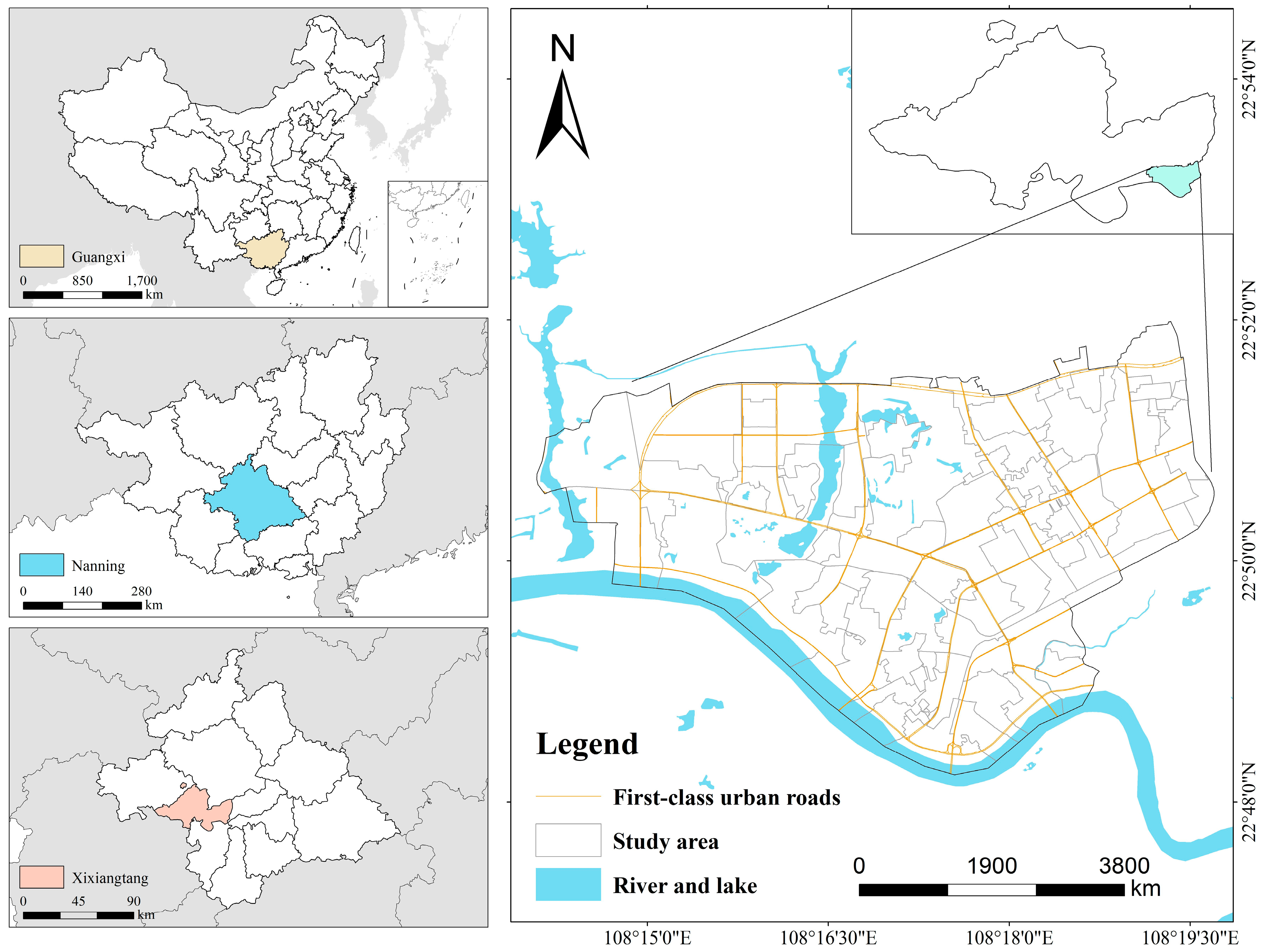
Figure 1. Location of the Study Area.
Ijgi 14 00362 g001
Figure 2. Workflow diagram of the study.
Ijgi 14 00362 g002
Figure 3. Spatial distribution of cardiovascular disease cases and annual statistics from 2020 to 2022. (a) spatial distribution of cases in 2020; (b) spatial distribution of cases in 2021; (c) spatial distribution of cases in 2022; (d) annual number of cardiovascular disease cases, 2020–2022.
Ijgi 14 00362 g003
Figure 4. Distribution Map of Total Cardiovascular Cases and LISA Cluster Map for Communities.
Ijgi 14 00362 g004
Figure 5. Spatial Distribution Characteristics of Built Environment Factors. (a) Population Density; (b) Building Density; (c) Road Network Density; (d) Number of Unhealthy Food Outlets; (e) Number of Healthy Food Outlets; (f) Number of Recreational Facilities; (g) Number of Public Transport Stations; (h) Facility POI Density; (i) Community Green Space Ratio; (j) Distance to Nearest Park or Square; (k) Distance to Nearest Metro Station; (l) Average Community Housing Price.
Ijgi 14 00362 g005
Figure 6. Comparison of Residuals in OLS, GWR, and MGWR Models.
Ijgi 14 00362 g006
Figure 7. Comparison of Bandwidths for Built Environment Variables between GWR and MGWR.
Ijgi 14 00362 g007
Figure 8. Boxplots of Significant Variable Coefficients and Mean Regression Coefficients for Each Variable.
Ijgi 14 00362 g008
Figure 9. Spatial Distribution Patterns of Regression Coefficients for Significant Variables. (a) Population Density; (b) Building Density; (c) Road Network Density; (d) Number of Unhealthy Food Outlets; (e) Number of Healthy Food Outlets; (f) Number of Public Transport Stations; (g) Facility POI Density; (h) Distance to Nearest Metro Station.
Ijgi 14 00362 g009
Table 1. Indicator System of Community Built Environment.
VariableDefinitionAbbreviationMeanStd.
Number of Cardiovascular CasesTotal number of cardiovascular cases in each community (persons)NCC61.9598.78
Population DensityPopulation density within the residential community, calculated based on China’s 100 m census grid data (10,000 persons/km2)PD3.121.22
Building DensityRatio of total building area to community area (ratio, 0–1)BD0.260.1
Road Network DensityTotal road length within the community divided by community area (km/km2)RND9.734
Land Use Mix EntropyLand use mix represented by entropy index (ratio, 0–1)LUME0.230.04
Number of Unhealthy Food OutletsNumber of convenience stores (including OK convenience stores) within a 500 m buffer zone around the community (count)NUFO44.9527.84
Number of Healthy Food OutletsNumber of vegetable markets, fruit markets, and integrated markets within a 500 m buffer zone (count)NHFO33.9920.4
Number of Recreational FacilitiesNumber of sports venues, swimming pools, chess rooms, fitness centers, etc., within a 500 m buffer zone (count)NRF13.7410.38
Number of Public Transport StationsNumber of bus stops and metro stations within a 500 m buffer zone (count)NPTS4.783.07
Facility POI DensityRatio of the number of various POI points to the community area (POIs/km2)FPOI1607.58900.3
Community Green Space RatioRatio of total green space area to community area (%)CGR13.638.07
Distance to Nearest Park or SquareDistance from the community to the nearest park or square (m)DNPS648.93461.72
Distance to Nearest Bus StopDistance from the community to the nearest bus stop (m)DBS244.23124.31
Distance to Nearest Metro StationDistance from the community to the nearest metro entrance (m)DMS762.68434.21
Average Community Housing PriceAverage second-hand housing price within the community (CNY/m2)ACHP7019.841117.32
Table 2. Summary Statistics, Multicollinearity, and Spatial Autocorrelation Tests for Variables.
VariableSummary StatisticsMulticollinearity TestSpatial Autocorrelation
MeanStd.ToleranceVIFMoran’s IZ-Valuep-Value
Number of Cardiovascular Cases61.95098.7800.2743.6540.2804.9840.000
Population Density3.1201.2170.3452.9000.3585.7070.000
Building Density0.260.0990.6481.5440.2143.5120.000
Road Network Density9.7303.9980.4202.3810.2083.4430.001
Land Use Mix Entropy0.2300.0440.4212.3750.0831.4960.135 *
Number of Unhealthy Food Outlets44.95027.8350.4442.2540.4306.9300.000
Number of Healthy Food Outlets33.99020.4000.5111.9580.3385.4320.000
Number of Recreational Facilities13.74010.3790.6111.6370.3986.4260.000
Number of Public Transport Stations4.7803.0700.2024.9450.3044.9730.000
Facility POI Density1607.580900.3000.5371.8620.1242.1270.033
Community Green Space Ratio13.6308.0700.7231.3830.1562.6140.009
Distance to Nearest Park or Square648.930461.7200.6561.5240.3125.1430.000
Distance to Nearest Bus Stop244.230124.3100.6171.6220.1011.7730.076 *
Distance to Nearest Metro Station762.680434.2100.6001.6650.5308.3820.000
Average Community Housing Price7019.8401117.3200.2743.6540.65110.5430.000
Note: * indicates that the variable did not pass the spatial autocorrelation test and exhibits spatial randomness.
Table 3. Comparison of OLS, GWR, and MGWR Model Results.
ModelR2Adjusted R2AICcRSSMoran’s I of Residuals for Each Model
Moran’s IZ Valuep Value
OLS0.3360.212928.05762.693−0.023−0.1730.863
GWR0.4950.292231.67438.899−0.066−0.9810.327
MGWR0.5320.348224.34836.065−0.058−0.8320.405
Table 4. Bandwidths of Variables in OLS, GWR, and MGWR.
BandwidthsOLSGWRMGWR
Intercept--7455
Road Network Density72 (93.50%)
Number of Public Transport Stations72 (93.50%)
Distance to Nearest Metro Station54 (70.13%)
Other Built Environment Factors76 (98.70%)
Table 5. Summary Statistics of MGWR Coefficients.
VariableMeanStd.MinMedianMaxNumber of Significant SamplesProportion (%)
Intercept0.0570.225−0.2670.0160.3912735.06
Population Density0.3540.0170.310.360.37677100.00
Building Density−0.2270.054−0.316−0.234−0.1512937.66
Road Network Density−0.1340.096−0.315−0.105−0.0082228.57
Number of Unhealthy Food Outlets0.2530.0220.210.2620.2794558.44
Number of Healthy Food Outlets−0.220.034−0.273−0.224−0.1462431.17
Number of Recreational Facilities0.1790.0240.1360.1810.2200.00
Number of Public Transport Stations−0.270.144−0.565−0.179−0.1412937.66
Facility POI Density−0.4020.032−0.452−0.405−0.33277100.00
Community Green Space Ratio−0.1490.024−0.196−0.146−0.11300.00
Distance to Nearest Park or Square−0.010.05−0.1310.0160.02500.00
Distance to Nearest Metro Station−0.220.069−0.345−0.208−0.1043241.56
Average Community Housing Price0.0320.044−0.0190.0120.13300.00
Disclaimer/Publisher’s Note: The statements, opinions and data contained in all publications are solely those of the individual author(s) and contributor(s) and not of MDPI and/or the editor(s). MDPI and/or the editor(s) disclaim responsibility for any injury to people or property resulting from any ideas, methods, instructions or products referred to in the content.