Lightweight Deep Learning Approaches for Lithological Mapping in Vegetated Terrains of the Vălioara Valley, Romania

Abstract

Mapping lithology in areas with dense vegetation remains a major challenge for remote sensing, as plant cover tends to obscure the spectral signatures of underlying rock formations. This study tackles that issue by comparing the performance of three custom-built lightweight deep learning models in the mixed-vegetation terrain of the surroundings of the Vălioara Valley, Romania. We used time-series data from Sentinel-2 and elevation data from the SRTM, with preprocessing techniques such as the Principal Component Analysis (PCA) and the Forced Invariance Method (FIM) to reduce the spectral interference caused by vegetation. Predictions were made with a Multi-Layer Perceptron (MLP), a Convolutional Neural Network (CNN), and a Vision Transformer (ViT). In addition to measuring the classification accuracy, we assessed how the different models handled vegetation coverage. We also explored how vegetation density (NDVI) correlated with the classification results. Tests show that the Vision Transformer outperforms the other models by 6%, offering a stronger resilience to vegetation interference, while FIM doubled the model confidence in specific (locally rare) lithologies and decorrelated vegetation in multiple measures. These findings highlight both the potential of ViTs for remote sensing in complex environments and the importance of applying vegetation suppression techniques like FIM to improve geological interpretation from satellite data.

1. Introduction

Lithological mapping plays a critical role in understanding the geological composition and distribution of Earth’s surface materials. This field is essential for applications such as mineral exploration, environmental studies, and land-use planning. Remote sensing data have long been the main basis for lithological classification [1,2,3]. The presence of vegetation, even in low densities, can introduce considerable noise in remotely sensed data, masking key geological features. This limitation necessitates advanced preprocessing techniques to reduce the influence of vegetation and sophisticated classification methods to improve accuracy. Modern remote sensing technologies and computational tools have opened new avenues for addressing these challenges, but the efficacy of these approaches varies with vegetation density and the methods employed.

This study explores the challenges and solutions in lithological mapping within vegetated areas, with a focus on preprocessing techniques, feature extraction methods, and classification algorithms.

1.1. Challenges in Lithological Mapping in Vegetated Areas

On bare soil, the lithological unit classification (LUC) is regarded as relatively straightforward [4,5,6]. The problem arises when the remotely sensed data is not optimal or when the research area is covered with medium- to high-density vegetation. Even a 10 percent grass cover can, in some cases, mask the spectral characteristics of the underlying materials [7]. This issue necessitates advanced preprocessing and classification techniques to extract additional insights from the data. In our research area, the Vălioara Valley in Romania, which we will describe in detail in a later chapter, we face precisely these challenges when we want to perform analyses to aid geological mapping.

To address the issues with the input data, it is preprocessed to correct the distortions that arise during data acquisition. This involves radiometric, atmospheric, and geometric correction of the data. Radiometric correction adjusts the data to fix errors in sensor sensitivity and record anomalies. Atmospheric correction removes the interference from satellite imagery, such as haze, dust, and vapors, that can alter the interpretation of the sensed data. Performing a geometric correction ensures that the data align accurately with geographic positions [8,9,10].

1.2. Preprocessing and Feature Extraction Techniques

The second part of preprocessing is feature extraction. In this phase, the data is enhanced to derive products and highlight features to aid classification, including spectral features like the Normalized Difference Vegetation Index (NDVI), mineral indexes, and topographic insights. NDVI is a computed index that indicates vegetation health and, on a larger scale, the distribution or temporal changes in vegetation, by comparing the red visible light and the near-infrared light reflected [11,12].

Vegetation affects remote sensing data spectrally and spatially. Understanding the underlying physical mechanism of such connection is crucial for designing preprocessing strategies. The spectral signature of green vegetation is characterized by the chlorophyll absorption in the red region and near-infrared wavelengths due to internal leaf structure [13]. These features can dominate the mixed pixels reflectance, especially in moderate to dense vegetation density.

Furthermore, vegetation introduces textural and shadowing effects, which may distort spectral homogeneity. To address this issue during preprocessing, rather than solely relying on model-based solutions such as deep learning, statistical correction methods can be effective, such as FIM. In addition, statistical evaluation tools can be used—such as a correlation analysis using indirect markers—to assess the effectiveness of vegetation suppression methods.

Mineral indices are computed to highlight the distribution of key minerals relevant to differentiate specific lithological units [14,15,16,17].

Indices derived from the digital elevation data can play significant roles in lithological classification [18,19]. Topographic features like slope and aspect are essential for comprehensive environmental and geographical analyses [20,21,22]. Texture features can also be crucial in the classification phase [23].

Spectral features from multispectral and hyperspectral datasets can be extracted by Principal Component Analysis [24], while polarimetric parameters and texture features can be extracted from Synthetic Aperture Radar (SAR) datasets [25]. The topographic data from the Shuttle Radar Topography Mission/Advanced Spaceborne Thermal Emission and Reflection Radiometer (SRTM/ASTER DEM) and aeromagnetic data can also contribute to overall classification accuracy [19,23,26,27]. The integrated approaches in which they used additionally derived textural, topographic, or geophysical components resulted in a significant improvement in overall classification accuracy. As a dataset enhancement, the Forced Invariance Method (FIM) can be used. FIM enhances the contrast in images by aligning the Digital Numbers (DN) of remotely sensed image bands with their corresponding vegetation index values. The goal is to normalize the influence of vegetation. While this method works particularly well in mixed arid and semi-arid areas, we assumed that it could also be useful in areas with mixed to high vegetation density [28,29].

1.3. Classification Techniques: Pixel-Based and Object-Based Approaches

Subsequently, the preprocessed data is processed with a classification algorithm. In classification, there are two main approaches: pixel-based image analysis (PBIA) and object-based image analysis (OBIA). In the case of pixel-based data processing, the classification algorithm analyzes every single pixel and assigns a label based on the pixel’s spectral signature [30]. On the other hand, an object-based approach uses a segmentation algorithm to group pixels into objects based on the texture of the input dataset and creates a specified number of segments [31]. Then, the information of the pixels is assigned to each segment/object, respectively. The objects are then classified [32]. The PBIA and OBIA approaches both have their own advantages and disadvantages. While OBIA yields higher accuracy measures, it requires better hardware resources, and the whole process takes significantly longer. Additionally, the segmentation based on textural features results in more information and less noise with the object-based approach than with the pixel-wise approach [33,34].

1.4. Machine Learning and Deep Learning Techniques

Lithological unit classification literature has a wide range of tested classification methods across areas with different vegetation coverage. There are three main types of machine learning methods that are used and considered as traditional machine learning-based classifiers. These are the RF (Random Forest), SVM (Support Vector Machine), and the SOM (Self Organizing Map) [15,24,32,35,36].

The traditional machine learning-based classification methods, SVM (Support Vector Machine) or RF (Random Forest), can achieve impressive results in semi-arid and moderately vegetated areas [26,35,37], while with the use of geochemical parameters, SOM was able to achieve satisfactory results [36]. However, the computation capacity needed and finetuning of the parameters is complex in the case of the SVM method, while the RF is sensitive to outliers and imbalanced datasets [2,25].

In the context of lithological classification, the mostly used DL classifiers include convolutional layers. The convolution can be one, two, and three-dimensional. The one-dimensional layers analyze the spectral depth of the dataset, while the two-dimensional layers focus on the spatial domain and handle the spectral bands as samples. The three-dimensional convolutional layer can capture spatial and spectral relationships; however, it requires significantly more computational power [38]. Comparing the different convolutional layers’ efficacy shows a significant gap in accuracies between the 1D and 2D layers, while the gap between the 2D and 3D layers’ performance is less in favor of 3D layers, in the case of arid areas. In the context of computation capacity, the order is reversed [39].

The other novel method in DL classification is the Vision Transformer-based classifiers. In a study with new implementation of the Vision Transformer, the FaciesViT in pure accuracy measures outperformed the convolutional networks and showed a better performance and generalization with a limited dataset [40]. In another study in lithology identification, the Rock-ViT model outperformed the convolutional layer-centered ResNet (Residual Network) while it was able to learn global patterns [41]. These models were tested on bare rock samples without the vegetation-induced noise factor. Improvements were made to the lithological classification in vegetation-covered areas by the authors using attention-based complex architecture models, reaching macro F1-scores above 60% [42]. In another study, the authors achieved significant improvements of over 5% compared to other techniques by using a multiscale dual attention approach [43].

In this study, the traditional methods are excluded, and the novel, deep learning-based classifiers are tested, along with a Multi-Layer Perceptron (MLP) as a reference point.

1.5. Primary Aim and Research Questions

The primary aim of this study is to test the three selected machine learning-based classifiers, the Multi-Layer Perceptron (MLP), the convolutional layer based Conv2D model, and a generalized version of Vision Transformer (ViT) efficacy on a mixed-vegetation-covered dataset. We also wanted to see how their ability to generalize changes when the dataset is modified with the vegetation suppression method (FIM), and how vegetation content affects the accuracy by correlation analysis. In parallel, the constructed models had to be as compact as possible to support the latest computational trends in lightweight, easy-to-use model structures. This would enable them to work in environments with limited resources while maintaining competitive generalizability.

The main questions specifically are as follows:

• How do the MLP, Conv2D, and ViT classifiers perform if applied to the selected mixed-vegetation-covered study area?
• What is the impact of the vegetation suppression technique FIM on the classification performance of MLP, Conv2D, and ViT models?
• How does the vegetation density (measured through NDVI) correlate with the classification accuracy of each tested model?

Based on the primary aims, this study aims to evaluate classification performance, analyze the impact of vegetation suppression, and understand changes in accuracy across different vegetation covers and classifiers. The secondary objectives are to compare the classifiers between different lithological units, identify the class-level impact of the FIM, and determine the optimal classification method for different vegetation coverage levels. Additionally, the aim is to achieve the accuracy of complex, deep learning-based models with our lightweight approach.

2. Materials and Methods

2.1. Study Area

The focal point of our study area is the Vălioara Valley and its broader surroundings, where a geological mapping project was recently launched with the aim of gaining a better understanding of the Late Cretaceous sediments found in the area [44,45]. The bounding coordinates of the 70 km² study area in the UTM34N metric cartographic coordinate system are as follows: easting min.: 635000, max.: 645000; northing min.: 5048000, max.: 5055000. The projection of the maps presenting the results of the analysis was also UTM34N, interpreted on the WGS84 datum surface.

The Vălioara Valley is located within the Hațeg Basin, which is one of the largest intermountain basins of the Southern Carpathians. The altitude in the center of the basin is 350 m. Due to its basin morphology, it is filled with Quaternary fluvial sediments in its central regions, which are accompanied by proluvial and colluvial sediments. Surrounding the basin, the Southern Carpathians are to the south, while to the west and northwest, the Rusca Montană mountain group is found, which is part of the Banat Mountains. To the east, the Sebes Mountains border the basin. The altitude of the mountain ranges exceeds 2400 m in the south, while in the east, the typical altitude is around 1500 m, and in the west, around 1000 m (Figure 1A). There is mixed-vegetation cover, characterized by forests, pastures, plantations, and open agricultural areas (Figure 1B).

Figure 1. Location and physiography of the study area: (A) geography, (B) true-color satellite image of the study area, and (C) general geology redrawn after the 1:200,000 geological map of Romania and other sources [45,46,47].

Figure 1. Location and physiography of the study area: (A) geography, (B) true-color satellite image of the study area, and (C) general geology redrawn after the 1:200,000 geological map of Romania and other sources [45,46,47].

The Hațeg Basin is a good example of a complex landscape, due to the geological evolution of the terrain. The geological structure of the region (Figure 1C) is shaped by large-scale over-thrusting of crystalline basement rocks linked to the Late Cretaceous phases of the Alpine orogeny [48,49,50]. During the early Late Cretaceous, a marine sedimentary basin, precursor to the Hațeg Basin, developed and accumulated primarily deep-marine siliciclastic turbiditic deposits, commonly referred to as “flysch” in the literature [46,50,51]. Overlying these marine deposits, the Haţeg Basin is filled with two main uppermost Cretaceous sedimentary units, the Densuş-Ciula and Sînpetru formations, both notable for their continental vertebrate fossils [44,47,52]. In the western part of the Haţeg Basin, where the study area is situated, the lower Densuş-Ciula Formation comprises coarse conglomerates interbedded with minor sandstones and mudstones. This lower sequence also includes tuff and volcaniclastic material derived from contemporaneous volcanic activity in the Banatitic Province to the west [53]. The middle section of the Densuş-Ciula succession features fluvial and proximal alluvial fan deposits, while the upper section, formed during the early to late Maastrichtian, also reflects predominantly alluvial depositional environments [54,55].

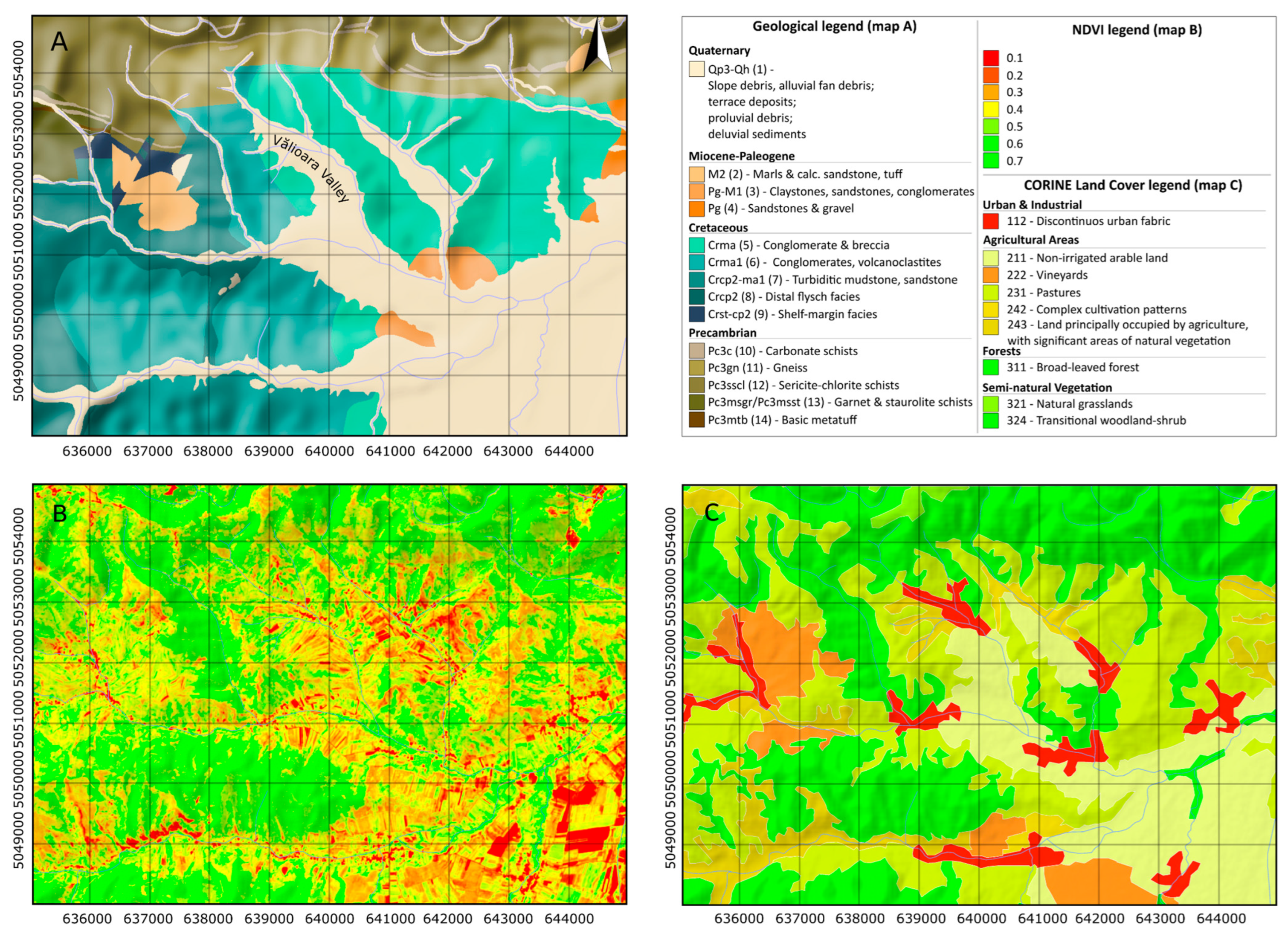
The study area was centered around the Vălioara Valley and the Densuş-Ciula Formation. In the northern part of the area, the morphology is higher, indicating the outcropping of crystalline rocks, while to the south, the upper Cretaceous sediments form the mountain ranges (Figure 2A). Quaternary formations are typically found in the valley floor and on the gentler slopes. It is a mixed landscape, including several small valleys such as Boita, Vălioara and Rachitova, and represents a 7 by 10 km (70 km²) area. The area includes elevated parts such as the eastern reaches of the Rusca Montană with the Curatului peak (Vârful Curatului), reaching a height of 939 m in the northern section, and Mount Fata (Dealul Fata), standing at 637 m, in the central to southern part. A local valley is also present in the southern region, beginning with the settlement of Demsuş and extending in a west–east orientation. The southeastern portion of the study area constitutes the plain area of the Hațeg Basin.

A wide variety of vegetation types, based on land use and natural distribution, are present in the study area. There is not a dominating species in this region. Meadows, farms, and forests are all equally represented in Corine land-use statistics [56] (Figure 2B).

Figure 2. Detailed maps of the study area: (A) geology based on 1:50,000 scale geological maps [57,58]; (B) the NDVI maps of the study area SD:2023.01.08, and (C) the CORINE land cover [56] (ID-s also in

Table 1. NDVI statistics of the study area delineated by CORINE land cover classes [56]. IDs correspond to areas on Figure 2B.

ID	Min	Avg	Max	CORINE Land Cover
112	0.052	0.421	0.640	Discontinuous urban fabric
211	0.051	0.423	0.679	Non-irrigated arable land
222	0.125	0.465	0.659	Permanently irrigated land
231	0.024	0.459	0.703	Pastures
242	0.102	0.454	0.650	Complex cultivation patterns
243	0.081	0.493	0.702	Land principally occupied by agriculture with significant areas of natural vegetation
311	0.071	0.559	0.701	Broad-leaved forest
321	0.324	0.478	0.644	Natural grassland
324	0.190	0.537	0.668	Transitional woodland/shrub

). The coordinate system and projection used is UTM N34.

Figure 2. Detailed maps of the study area: (A) geology based on 1:50,000 scale geological maps [57,58]; (B) the NDVI maps of the study area SD:2023.01.08, and (C) the CORINE land cover [56] (ID-s also in Table 1). The coordinate system and projection used is UTM N34.

The NDVI analysis revealed variations in the density and health of the vegetation, with darker green areas denoting strong vegetation, which is primarily seen in the vast forest sections, as indicated by the CORINE land-use data as well (Figure 2B,C). The NDVI is created from a satellite image taken in fall of 2023, so the forested areas also reflect a lower density than during the growing season. Despite this, the forested areas can still be identified through visual evaluation.

Meadows, interspersed between forested regions, can also be delineated on the NDVI, occupying the middle of the NDVI value range, represented in white to light green colors. Although meadows do not grow tall, they can be dense, preventing light from reaching and reflecting from the soil. Grass also falls into this reflection category, which can significantly overlap but can be slightly distinguished from meadows on the NDVI (Table 1; NDVI values). Farmland usually exhibits high NDVI values. This is because most of the fields are harvested in the autumn, but some crops are still present in certain areas. The farmlands, being partly prepared for winter, appear in vigorous red, representing one extreme of the vegetation range with high soil reflectance. Additionally, the parts of the cultivated area that still have crops fall into the mid-density range of vegetation. Residential areas exhibit higher reflection values attributable to two main reasons. Human-built structures reflect more light because of the materials used in roofs and pavements. The other reason is managed vegetation: households maintain their land by activities like mowing the grass. Also, next to residential areas, there are orchards. In orchards, the trees are planted in a pattern that results in a more homogeneous NDVI distribution. The water coverage is not significant (hidden by vegetation) in the study area, and the satellite images used are cloudless, so the NDVI values are within the 0 to 1 range.

Table 1 presents the NDVI ranges for various CORINE land cover classes revealing patterns and land-use characteristics. Discontinuous urban fabric and non-irrigated arable land share similar NDVI averages (~0.42), indicating moderate vegetation cover. Permanently irrigated land, pastures, and complex cultivation patterns show slightly higher average NDVI values (0.45–0.46), reflecting consistent agricultural activity. Lands that are dominantly used for agriculture and those that contain natural vegetation, also next to broad-leaved forests, stand out with the highest average NDVI values (0.493–0.559, respectively), introducing robust canopy cover. Natural grasslands and transitional woodland/shrub categories are represented in high averages, while grasslands fit in between the pastures and cultivated areas, the transitional lands are closer to the broad-leaved forests [56].

2.2. Data Collection

On the input side, we had three different kinds of datasets. We used Sentinel-2 multispectral time-series data as the base, SRTM elevation data, and lithological information derived from published geological maps as ground truth [57,58]. The multispectral images were in L2A format, indicating they already have radiometric, atmospheric, and geometric corrections applied. In the preprocessing, the original 12 bands were used with their original spatial resolution (

Table 2. Sentinel-2 image bands and parameters (spatial resolution and central wavelength) [59].

Band Number	Spatial Sample Distance (m)	Central Wavelength (nm)
1	60	443
2	10	490
3	10	560
4	10	665
5	20	705
6	20	740
7	20	783
8	10	842
8a	20	865
9	60	945
10	60	1375
11	10	1610
12	10	2190

). To maintain the same pixel size, in both the geological data and Sentinel-2 data, only a spatial resample is used (on Sentinel-2 imagery), while the spectral values remain unchanged within the area of the original pixel size.

The time-series collection consists of six different images. This collection covers the entire vegetation period of the study area, containing images from each season.

The dates of the images are

• 2021-02-25;
• 2023-01-08;
• 2023-04-28;
• 2023-11-02;
• 2023-12-19;
• 2023-12-27.

There is one image from 2021 and the others are from 2023. The aim of this multi-season collection was to gather as much information as possible from the vegetation cover and from the reflectance mix of the vegetation and soil (winter). The images were downloaded from the Copernicus Datahub using the Semi-Automatic Classification plugin in QGIS. All the acquired images are cloudless and contain minimal to no distortions over the study area.

The SRTM dataset gives additional topographic context to the classifier and supports a deeper understanding of the study area. The SRTM data was also resampled to match with the corresponding input dataset.

Lithological maps were used to train and validate the classification (supervised classification). We used 1:50,000 scale maps published by the Romanian Geological Institute as a geological basis. The research area includes two sheets, which were produced in two different mapping periods, resulting in differences in key elements. The greater part of the defined area is covered by the Hațeg sheet [57], while the western area extends into the Băuțar sheet [58]. Both sheets were compiled from several geological surveys conducted in the second half of the 20th century. The 1:200,000 scale maps of the area are available online in vector form on the website of the Romanian Geological Institute; however, 50,000 sheets cannot be accessed in this form. For this reason, the processing of the lithological maps involved vectorizing the raster format maps and unifying the geological units by creating categories based on lithological similarities (

Table 3. Lithologies of the study area based on 1:50,000 scale geological maps and other studies [45,57,58].

Index	Lithology Type	Class
Qh2	Slope debris, alluvial fan debris	1
Qh1	Terrace deposits at height of 2–4 m	1
Qh1pr	Proluvial debris	1
Qp3-Qh	Flood deposits	1
Qpf7	Terrace deposits at height of 15–20 m	1
Mm2	Marls, sands, and fossiliferous calcareous sandstone with tuff interlayers—Delinești Formation	2
Pg-M1	Gray claystones, red sandstones, and conglomerates	3
PPg	Sandstones and gravel	4
Crma	Conglomerate, breccia, and coarse sandstones with purple and black siltstones with coal interlayers (Densuş-Ciula Formation, middle and upper parts)	5
Crma1	Conglomerate, sandstone, siltstone, volcaniclastics, lavas, and andesitic tuffs (Densuş-Ciula Formation, lower part)	6
Crcp2-ma1	Marls/mudstones + siltstone, sandstones, sandy calcarenites, and microconglomerates; flysch facies, predominantly distal (Pui Formation)	7
Crcp2	Marls/mudstones + siltstone, sandstone, and calcareous sandstone, in fine- to medium-grained layers; distal flysch facies	8
Crst-cp2	Marls/mudstones, calcareous marls, and marly silty, gray, whitish, and locally quartzose sandstone; shelf margin and hemipelagic facies	9
Pc3c	Carbonate schist + dolomite	10
Pc3gn	Gneiss	11
Pc3sscl	Sericite-chlorite schists	12
Pc3msgr	Garnet (almandine) mica schist	13
Pc3msst	Garnet and staurolite mica schist	13
Pc3mtb	Basic metatuff	14

). The created categories were used as classes for classification; each class has a different label (1–14).

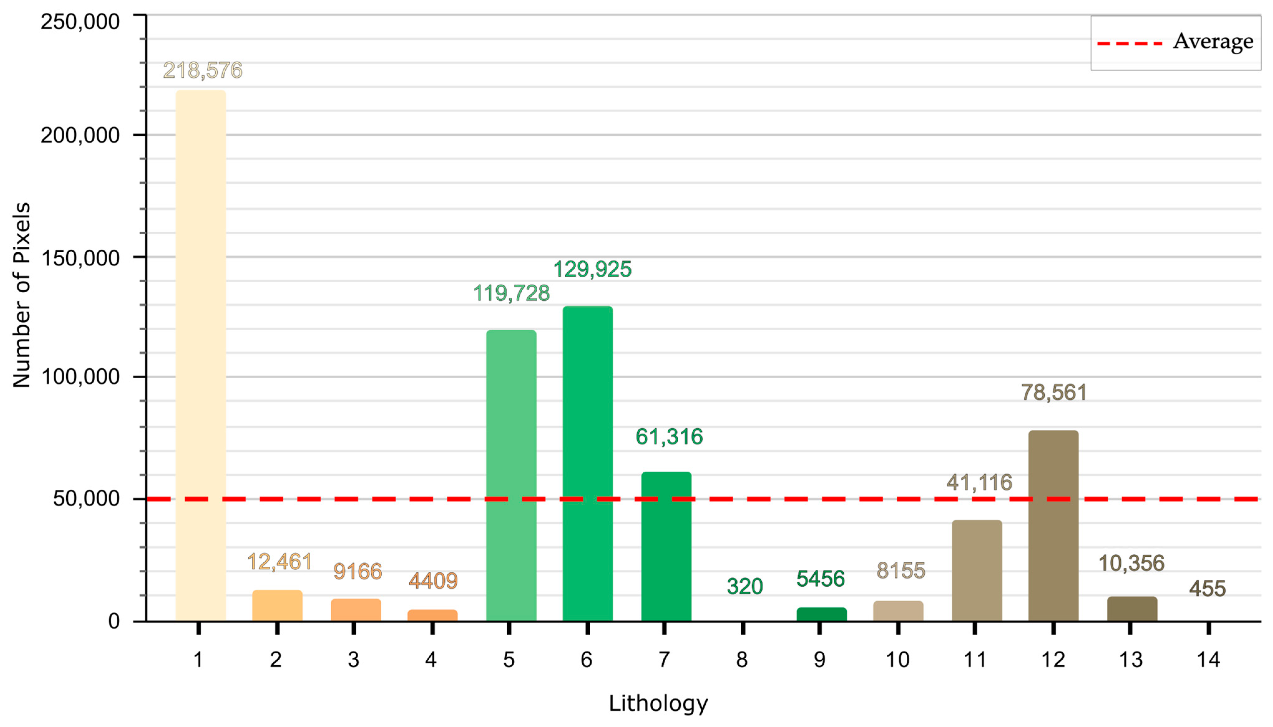
Sampling was performed on the digitized geological map, but since the processing was pixel-based, the vector format was re-rasterized. In the case of lithological maps, the pixel size was chosen to match the Sentinel-2 datasets (10 m spatial resolution). The lithological units are represented by a different number of pixels for each lithological type. There are dominant classes with great coverage, such as class 1 (218,576 pixels), which includes slope debris, alluvial fan debris, and different terrace deposits. This is followed by Cretaceous units, such as class 6 (129,925 pixels) and class 5 (119,728 pixels). This indicates the dominance of sedimentary rocks. The least dominant features in the examined area are class 8, (distal flysch facies) and class 14 (basic metatuff), with only 320 and 455 pixels, respectively. There are other classes showing moderate representations, with pixel counts ranging from 4400 (class 4) to 78,561 (class 12).

Figure 3 shows the number of pixels for each defined class. Classes 8 and 14 have significantly fewer pixels than the average number per class (~50,000 = 700,000/14). While classes 3, 4, 9, and 10 have solid coverage and are an order of magnitude higher than 8 and 14, they are still less than average. Class 2 has a sample size of the same order of magnitude as the average, but it is a fraction of it. 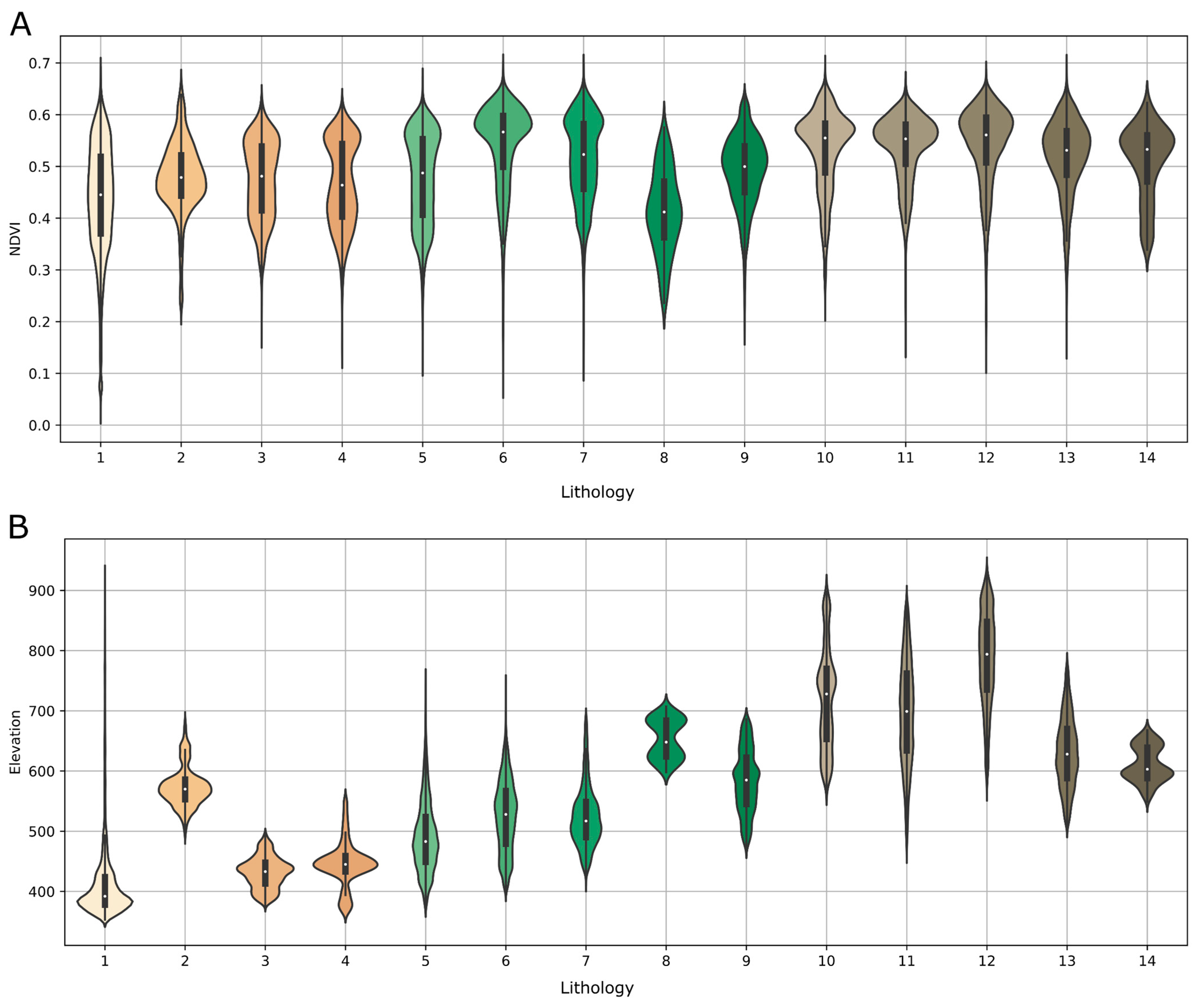The NDVI values for each class are shown in Figure 4A. Concerning the trend, the lowest median NDVI is observed on Quaternary deposits (class 1). Values generally increase and peak on Cretaceous flysch and conglomerate units (classes 6 and 7) before remaining consistently high across the metamorphic rocks (classes 9–13). Concerning the distributions, the lower-indexed classes like class 1 and class 5 cover a larger extent of the NDVI scale, and their shapes are more elongated. In contrast, most of the higher-indexed classes (>8) show distributions that are more tightly clustered at the higher end of the NDVI scale. Class 8 is a notable outlier, displaying a median NDVI that is lower than any other class and a very narrow distribution.

For classes with a relatively low number of samples and higher vegetation values, the risk of low accuracy is high. In these cases, the classification model’s ability to distinguish lithology, and consider vegetation has a greater impact on performance. In other words, in these classes, the right choice of method can lead to significant improvements.

The spatial distribution of lithological units in the study area is closely related to topography. A clear altitude-based differentiation of rock types is observed (Figure 4B), which is a major geo-environmental feature of the region and other areas in general [60,61,62]. The low-elevation zones, which are primarily below 500 m, are dominated by Cenozoic sedimentary rocks. These include Quaternary deposits such as alluvium and terrace deposits (class 1), as well as Neogene marls, sands, and claystones (classes 2–4). The violin plots for these rock types are compact and concentrated at lower altitudes, indicating that they occupy a narrow and distinct elevation range. At intermediate and higher elevations, the lithology is more varied. Cretaceous units, including conglomerates, sandstones, and flysch facies (classes 5–9), are distributed across a broad elevation range, typically between 400 and 700 m. The highest elevations in the study area, generally above 600 m, are composed of Palaeozoic metamorphic rocks. Specifically, carbonate schist (class 10), gneiss (class 11), and other schists (classes 12–13) are found at these higher altitudes. The plot for gneiss (class 11) indicates that it forms the highest peaks. Less represented classes (8, 14) have a very narrow elevation range, resulting in a unique violin-like shape.

2.3. Preprocessing and Feature Extraction

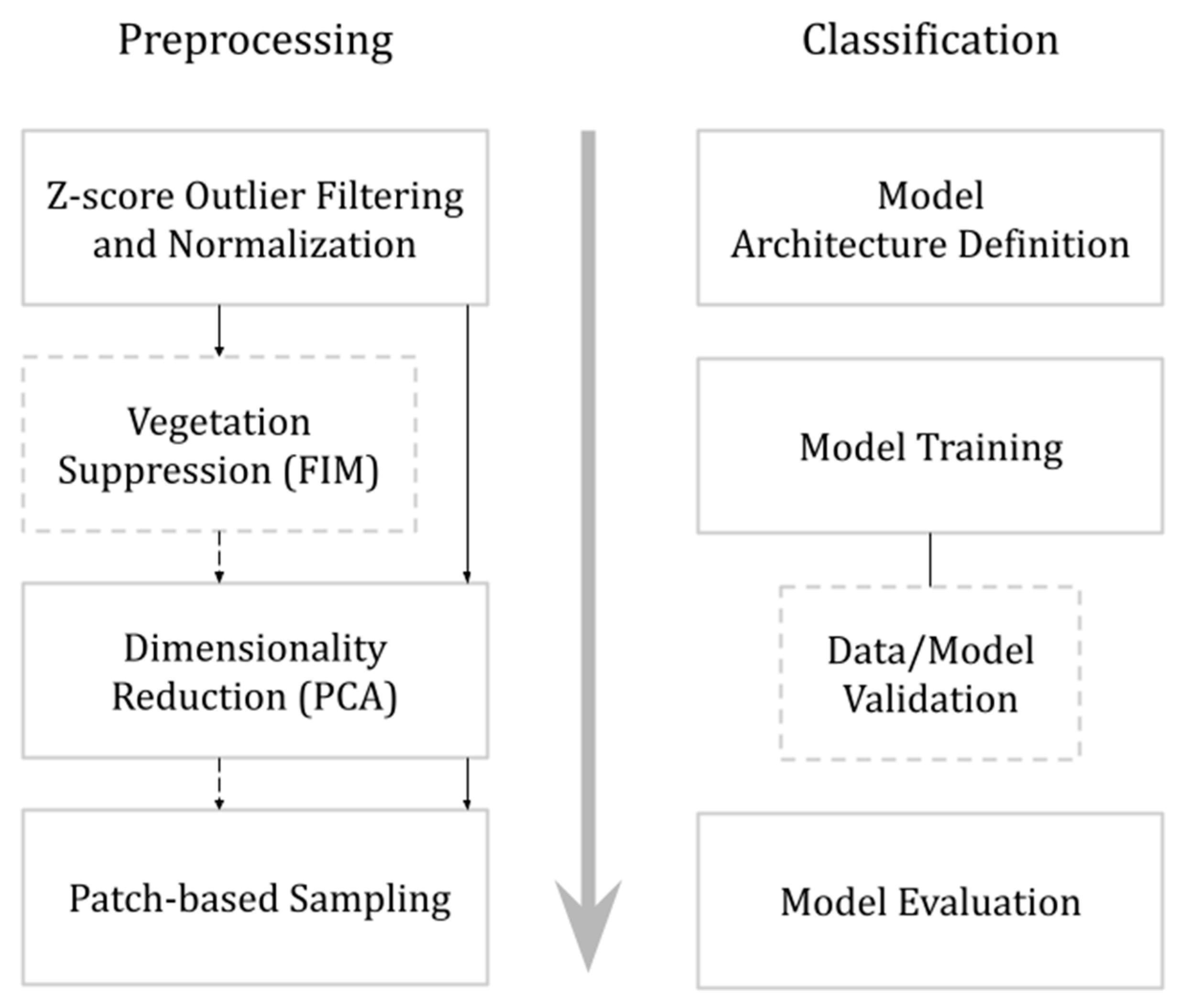
In this section, we outline the key steps of data processing from the loading to the full image prediction including the description of the Forced Invariance Method. The data pipeline was separated into two parts: the preprocessing and classification (classifier) parts (Figure 5).

During the preprocessing part, the main goal was to create a normalized, unbiased, outlier-, and noise-free dataset in a specific shape the classifier can work with. The data normalization and concatenation are the first step of data processing, ensuring the images are combined and interpreted on the same scale (including the handling of outliers).

All Sentinel-2 bands with native 20 m and 60 m resolutions were included in the analysis. The 60 m bands (B1, B9, and B10), which were designed for atmospheric correction, were also incorporated. As part of the preprocessing, these bands were resampled to a 10 m spatial resolution to match the highest resolution bands. To achieve this, the nearest neighbor interpolation method was used, which is a frequently used technique to bring different spatial resolution bands to the same pixel number while new, interpolated values are not calculated [63,64,65].

The SRTM elevation data went through the same normalization and outlier filtering until it was combined with the satellite imagery collections after the Forced Invariance Method was applied (dataset wise). The Forced Invariance Method (FIM) was one of our main preprocessing steps, particularly to test its capabilities in suppressing vegetation and revealing underlying lithological features. After the FIM, each advancement on the flowchart (Figure 5) is performed with the original dataset and the FIM modified dataset. As a noise reduction and data compaction technique, the Principal Component Analysis (PCA) is included. The final step of the preprocessing pipeline is patch extraction. This step arranges the data so there will be no overlap between the train and validation datasets, and it also forms the input shape that fits the classifier.

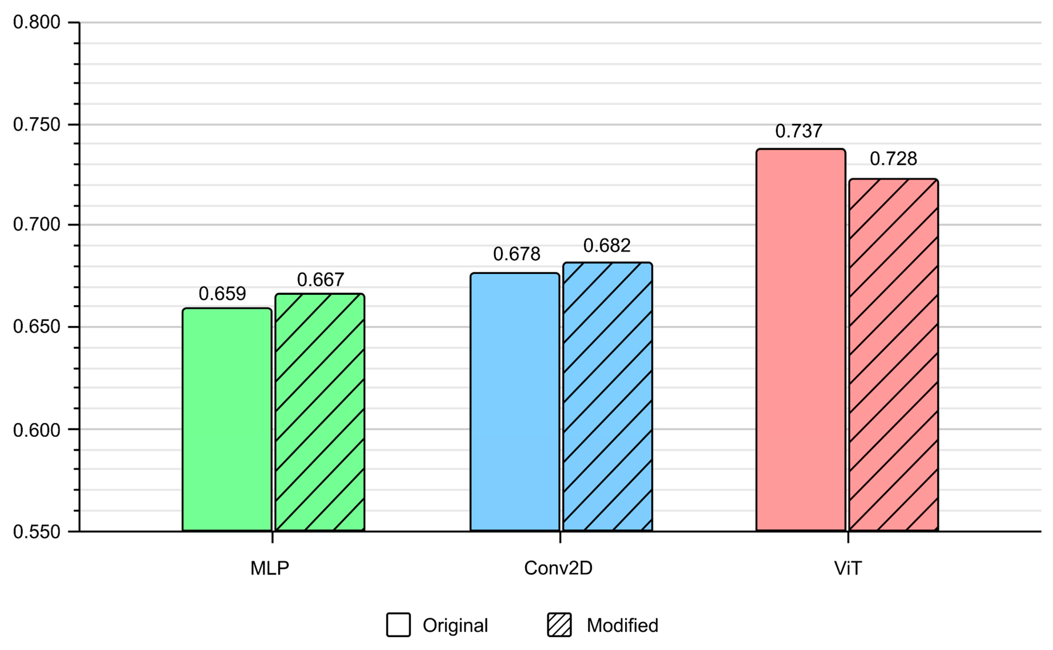
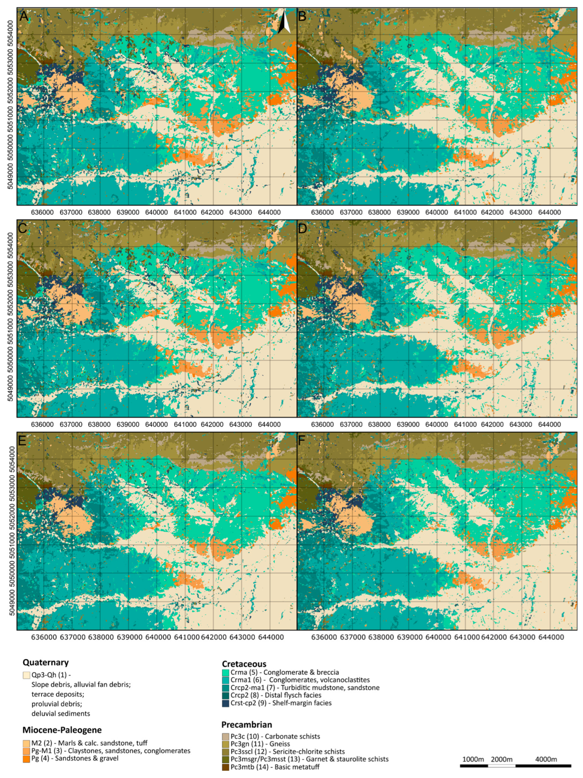
The second part of the methodology is where the framework definitions of the classifiers are made. Three different model definitions have been created: an Artificial Neural Network (ANN)-based Multi-Layer Perceptron (MLP), a convolutional layer-centered (Conv2D), and a Vision Transformer-based one (ViT). Each model handles the dataset differently, so during the training part, the number of (all) parameters and processors are different, though they share the same training parameters (outside the model definitions). As part of the training, we validated the datasets and models by monitoring the training and validation loss measurements. The trained models were then used to predict the whole input satellite images. The results are evaluated with common measures, like the F1-score and Overall Accuracy (OA), and practical measures, like vegetation category-based F1-scores (as trend charts), the vegetation index, and F1-score correlation (bar plot). Maps were also created for visual interpretation.

2.3.1. Z-Score Outlier Filtering and Normalization

The initial preprocessing stage involved outlier removal and data normalization to ensure all input features are interpreted on the same scale. First, the time-series data were loaded using the Python GDAL library, which is an efficient module that has tools to handle geospatial meta information of raster-type datasets. After the time-series data is loaded (each instance individually), the geospatial metadata (e.g., projection and geotransform parameters) from each source file was preserved in order to ensure the final outputs could be geolocated correctly. Next, a z-score-based outlier filter was applied to the time series to identify and remove statistical outliers. Outliers are data sequences not fitting in the dataset and causing performance loss later. This step was critical, as certain downstream algorithms in the processing pipeline, particularly the Forced Invariance Method, are sensitive to extreme values, which can lead to analytical instability and degrade performance [66].

Following outlier removal, a simple min–max normalization technique was used, and the data were scaled to a uniform range of 0–1. The SRTM elevation data also went through the same outlier filtering, but it was processed separately. After this step, the instances were in the same shape and on the same scale, and the normalized time-series layers were stacked to form a single, multi-dimensional data array.

2.3.2. Vegetation Suppression (FIM)

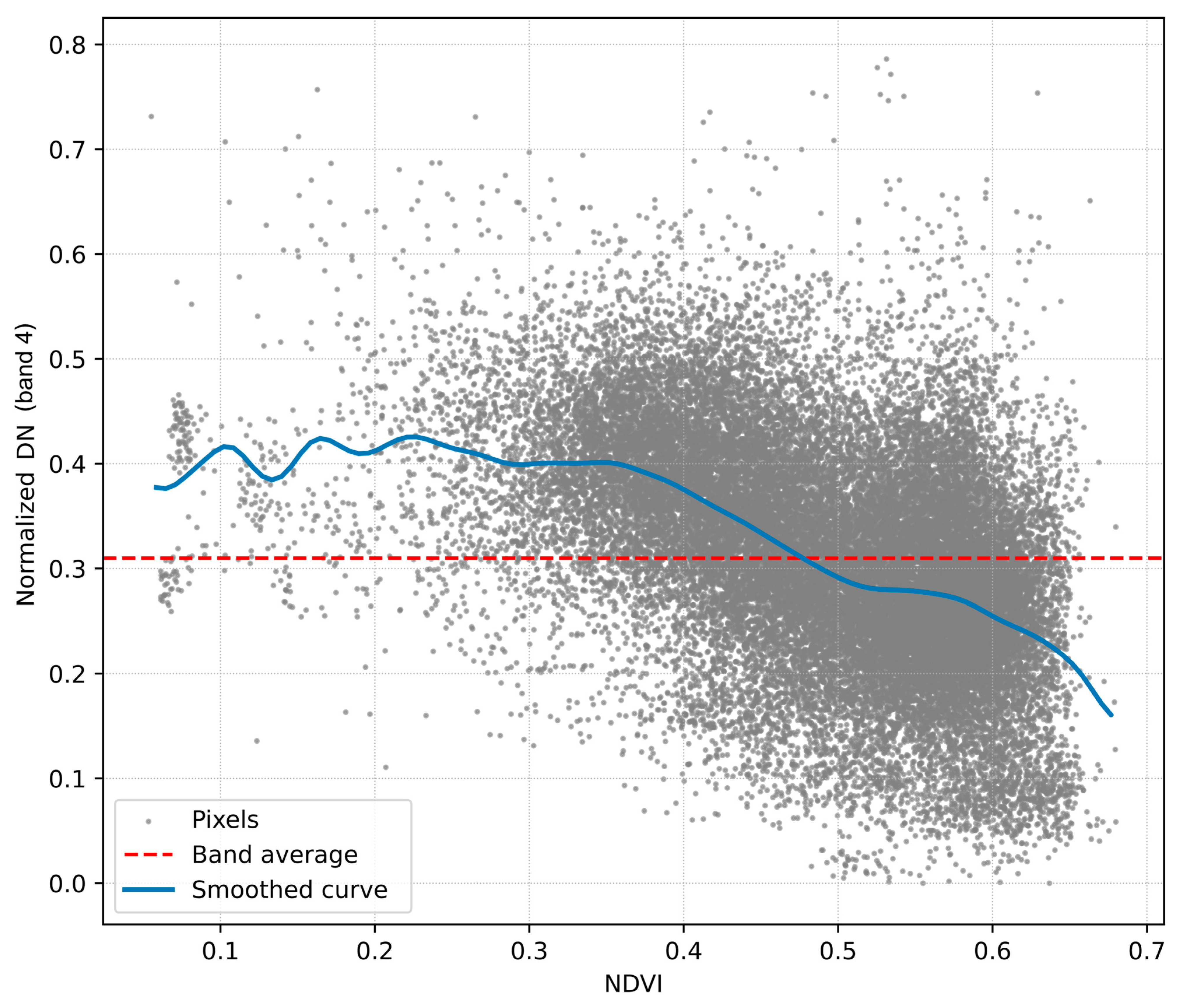
The Forced Invariance Method involves preprocessing the data by applying dark pixel correction, subtracting the smallest DN (Digital Number) value pixels from all pixels in each band to correct atmospheric path radiance and sensor calibration offsets. The vegetation index calculation is the second step, NDVI (Normalized Difference Vegetation Index) by default, used to plot against each band on a scatter plot (Figure 6). Average DN values represent the trend over NDVI categories, which is described with the best fitting curve. Median and mean filters are suggested by the authors of the FIM study [28] for curve fitting. With the known connection between the band values and the NDVI trend, the curve can be flattened with the following equation [28]:

$$PixelD{N}_{new}=PixelD{N}_{original}\times {\displaystyle \frac{TargetDN}{CurveD{N}_{VegetationIndex}}}$$

(1)

The TargetDN is an adjustable variable, corresponding to the average DN value for each band by default. Following these steps, the vegetation-related contrast is neutralized, with only the lithological patterns remaining and the other terrain-specific information. Additional steps like radiometric outlier masking to exclude anomalous radiometric features are advised. Post-processing, like contrast stretching and color balancing, is also included in the original study [28].

After this step, the workflow continued with two different datasets: the one modified with this method (FIM-modified dataset), and the one that skipped this step (original dataset). The SRTM elevation data is concatenated with the resulting flattened dataset—the original dataset is also extended with the same SRTM elevation data.

For each satellite image, the corresponding NDVI was calculated and used for the decorrelation. Additionally, the NDVI values were downscaled to the corresponding band’s resolution, ensuring there was no distortion in the average NDVI and band DN values.

2.3.3. Dimensionality Reduction

During the Principal Component Analysis of multiband rasters, the dataset size is reduced, while the variability within is mostly retained. The process involves the calculation of the covariance matrix, where each element represents the relationship between two bands. This covariance matrix undergoes eigen decomposition to yield its corresponding eigenvalues and eigenvectors. Each eigenvalue represents the variance explained by a single component, and the eigenvectors define the linear combinations of the original bands. The eigenvalues are then ranked in descending order, and the principal components are generated by projecting the original data onto the axes defined by these ranked eigenvectors [67].

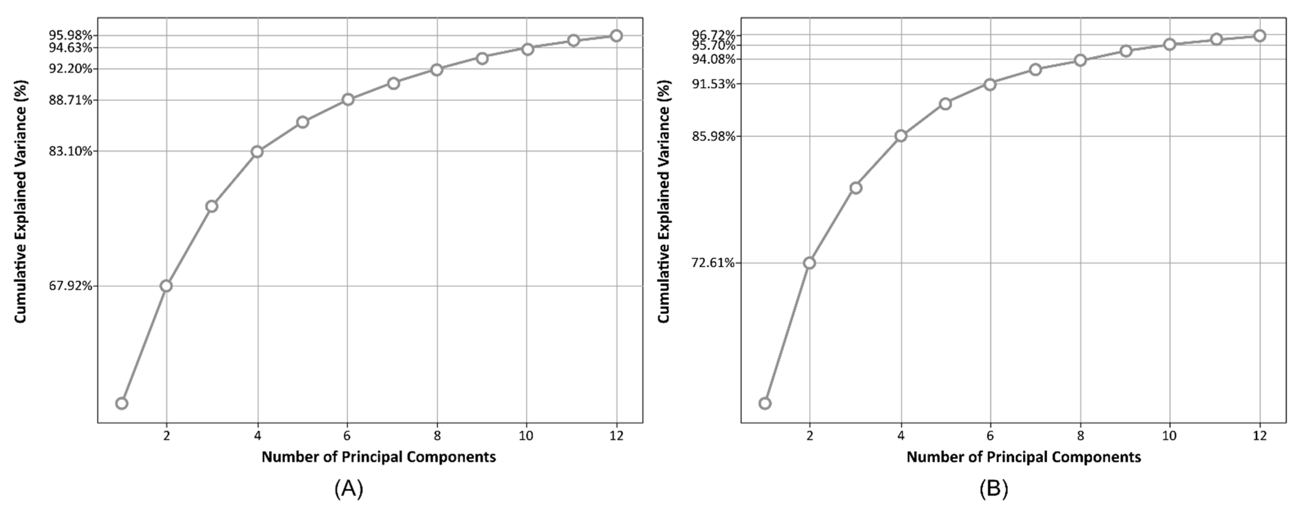
Dimensionality reduction involved 73 input features. These features included 72 bands from the satellite time series (6 dates × 12 bands per date) and one band from the SRTM. The criterion for selecting the number of principal components (PCs) was the cumulative explained variance (Figure 7), which explains the retained variability of each principal component. The first 12 principal components were selected for both the original (A) and decorrelated (FIM) datasets. This number of components accounts for a very high percentage of the total data variability in both scenarios: 95.98% for the original dataset and 96.72% for the FIM-processed dataset.

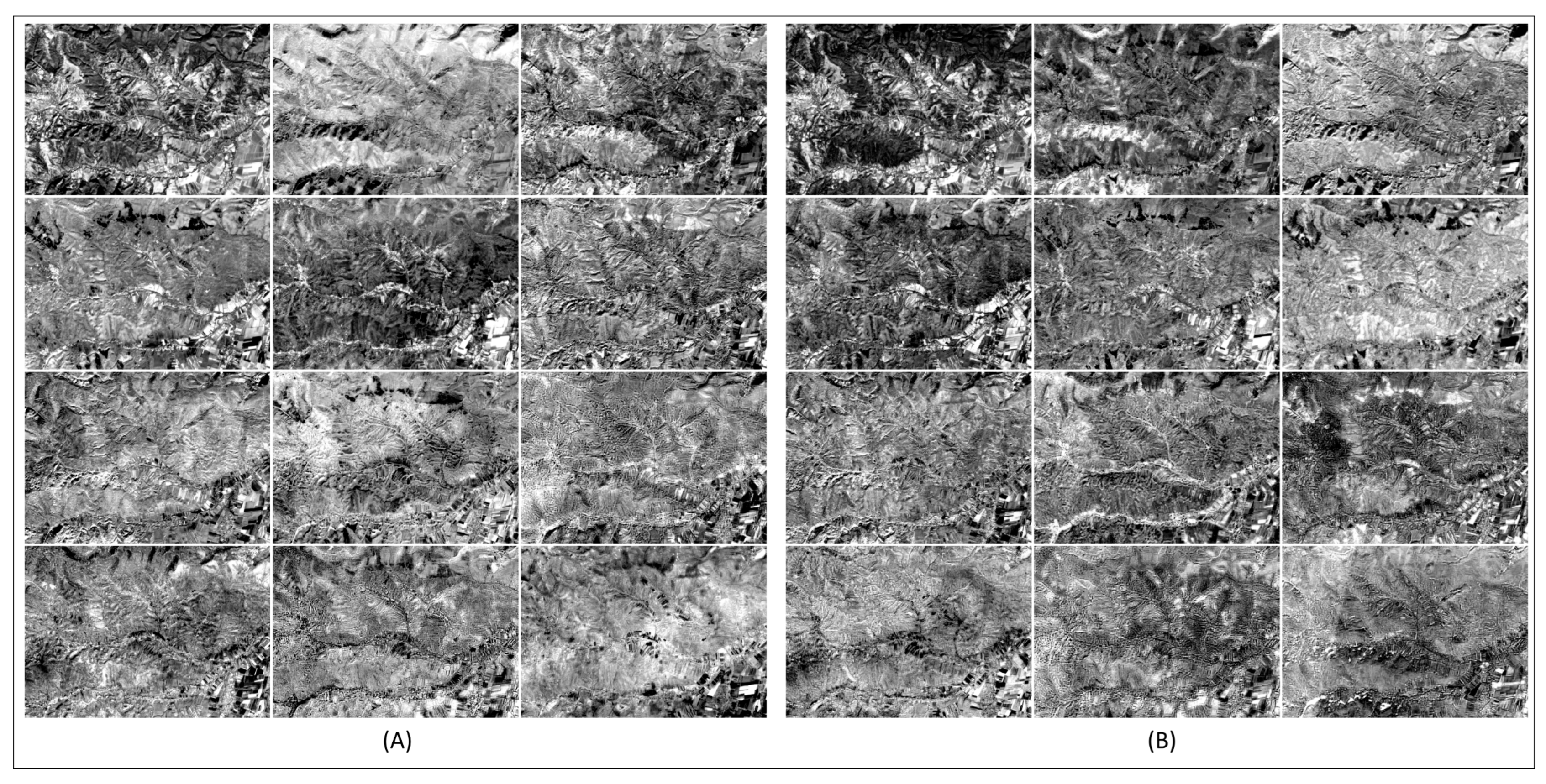
The FIM-processed data (Figure 7B) shows a marginally higher cumulative variance than the original data (Figure 7A). This is likely due to the modification reducing the overall data complexity, allowing for more of the total variance to be captured in fewer components. To ensure consistency between the two processing workflows, we used the 12 output bands for both datasets. The 12 output bands for both datasets are represented in Figure 8.

The comparison between band-wise contributions to the PCA output revealed notable shifts between the original and the decorrelated datasets (

Table 4. Summarized contribution of bands across images to PCA output.

Band	Normalized Contribution (Original)	Normalized Contribution (Modified)
B8	0.179	0.221
B12	0.159	0.167
B7	0.137	0.153
B10	0.130	0.094
B9	0.113	0.102
B6	0.109	0.118
B11	0.069	0.043
B5	0.042	0.038
B4	0.032	0.022
B3	0.017	0.020
B2	0.010	0.018
B1	0.003	0.002
SRTM	0.001	0.001

). In both cases, bands B8, B12, and B7 were the most informative. In the modified dataset, the value of band B8 increased from 0.179 to 0.221; the values of bands B12 and B7 also increased. The additional values of the other bands were less significant, though the order changed between the two datasets. Every other band lost significance when the dataset was modified, except B3, B2, and B1. This suggests that decorrelation suppresses some redundant spectral information while enhancing the relevance of others, with the order remaining almost the same. The low contribution of SRTM in both cases is expected, though it is also present in the results.

The distribution of information content across satellite scenes showed major reorganization in the modified dataset compared to the original, considering the acquisition date (

Table 5. Summarized contribution to PCA output of each satellite image.

Sentinel-2 Date	Normalized Contribution (Original)	Normalized Contribution (Modified)
2023.04.08	0.223	0.416
2023.01.08	0.179	0.182
2023.12.27	0.178	0.070
2023.12.19	0.165	0.062
2023.11.02	0.142	0.076
2021.02.25	0.113	0.193
SRTM	0.001	0.001

). The scene acquired on 8 April 2023 retained the highest variance; the significance of this scene almost doubled with the FIM preprocessing, and it was the only scene that did not change position in terms of significance. This increase may indicate a clean or vegetation-contrasting scene, which the FIM preserves more effectively. After preprocessing, the 8 January 2023 image lost second place, while the extracted information content grew. The importance of other scenes decreased.

2.3.4. Patch-Based Sampling

The last step of preprocessing is to incorporate spatial and spectral contexts for the classifier. To provide contextual information for each training sample, a square window of pixels was created around each central pixel. The mask creation for training, evaluation, and hold-out datasets followed strict rules. The hold-out set is preserved for final validation, as there must be an unseen portion of the dataset. The hold-out dataset is used to evaluate the robustness and generalization capabilities of the models.

Pixel-Based Image Analysis with the extraction of contextual patches can involve data leakage. If the training and validation patches are selected too close to one another, their areas can overlap. This allows the same pixel data to be present in both the training and validation sets, leading to artificially inflated performance metrics and a model that cannot generalize well to truly unseen data [68].

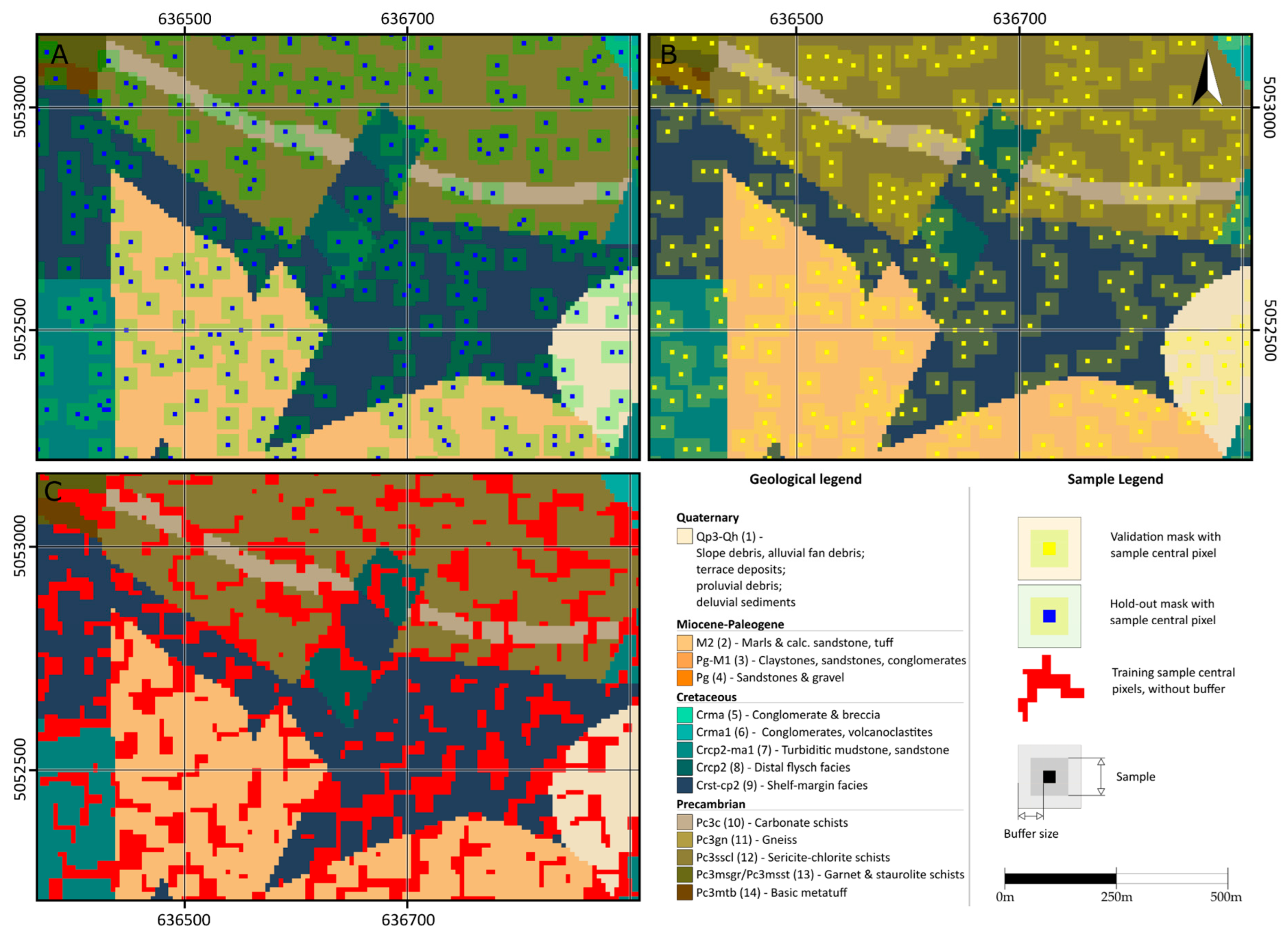
To prevent this, a spatially disjointed sampling strategy was implemented. During mask creation, the distribution of the pixels was random, stratified by lithology to ensure all classes were represented (Figure 9A). A buffer zone was applied around each validation pixel to define the validation patch and create a “keep-out” zone for training samples (Figure 9B). Training samples were then selected from the remaining areas, guaranteeing they were spatially separate from any validation patch (Figure 9C). In this study, validation and hold-out split masks were defined as a 5 × 5 pixel window, created by using a 2-pixel buffer around the central pixels of the samples (Figure 9).

Firstly, the hold-out dataset’s central pixels were chosen, and a 2-pixel buffer was applied around them. Approximately 1.6–2.2% of the pixels were chosen for hold-out for each lithological unit within each class. For the validation set, additional pixels were selected from the remaining pool, also stratified by lithological class. All remaining available pixels became part of the training set. For each dataset, masks were created. The sample ratio of the training, validation, and hold-out datasets is approximately 84-8.5-7.5, respectively (

Table 6. Number of samples per lithological class for the training, validation, and hold-out sets.

Class	Total Pixels	Training Samples	Validation Samples	Hold-Out Samples
1	218,576	42,819	3928	3474
2	12,461	3025	290	251
3	9166	2312	215	185
4	4409	1057	111	91
5	119,728	29,225	2698	2403
6	129,925	31,791	2895	2602
7	61,316	15,086	1390	1229
8	320	77	10	7
9	5456	1380	139	112
10	8155	2161	290	179
11	41,116	10,238	945	823
12	78,561	19,445	1830	1589
13	10,356	2472	269	212
14	455	117	13	11

).

This approach preserves the spectral profile of the central pixel and provides additional spatial information on spectral and topographic properties.

During sample generation, the edges were also used as central pixels. To overcome the edge effect and be able to predict near the edges during the inference, we used reflect padding. Reflect padding is a widely used technique, which extends images over the edges by mirroring the pixel values. This method improves classification accuracy by preserving the local texture and spatial consistency near the image boundaries [69].

2.4. Model Architectures

In this study, three different deep learning classifiers were tested: a Multi-Layer Perceptron (MLP) with dense layers for processing, a Conv2D model that utilizes only convolutional layers for processing, and an implementation of the Vision Transformer (ViT) architecture. For each model, batch normalization and dropout layers were also used to ensure the models have no biases and improve the generalization capability on unseen data.

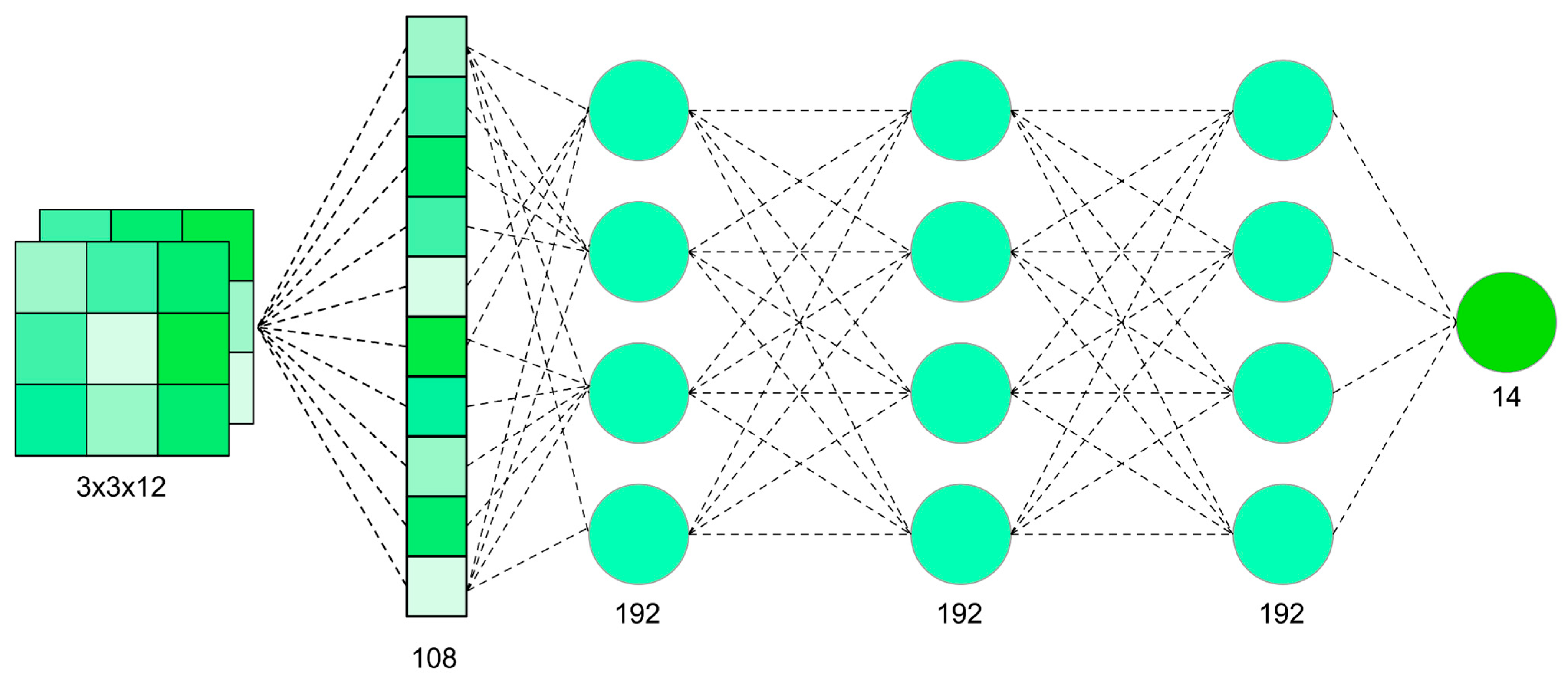
The MLP is the simplest among the classifiers tested. It used three hidden dense layers (192 nodes each) and an output dense layer (14 nodes) with SoftMax activation, which converted the outputs into a probabilistic interpretation [70]. For each layer, the ReLU (Rectified Linear Unit) activation function was added to introduce non-linearity into the model (Figure 10). During training, each pixel’s information is considered. The MLP model benefits from the additional contextual information introduced by the window-based approach. However, it requires flattened input, so the positions of pixels are not preserved across the layers. The purpose of this model was to serve as a performance baseline for comparison.

The second model was a Convolutional Neural Network (CNN), which used three two-dimensional convolutional layers for processing. Each layer consisted of 192 filters (feature maps) as parameters, and we also used padding (same; differs from the patch extraction). Using padding preserves the spatial dimensions of the feature maps throughout the convolutional blocks, thus avoiding data loss [71]. The filter sizes were 2 by 2 in all convolutional layers, which also ensures there is no lost data. Before the output layer, the feature maps were flattened (Figure 11).

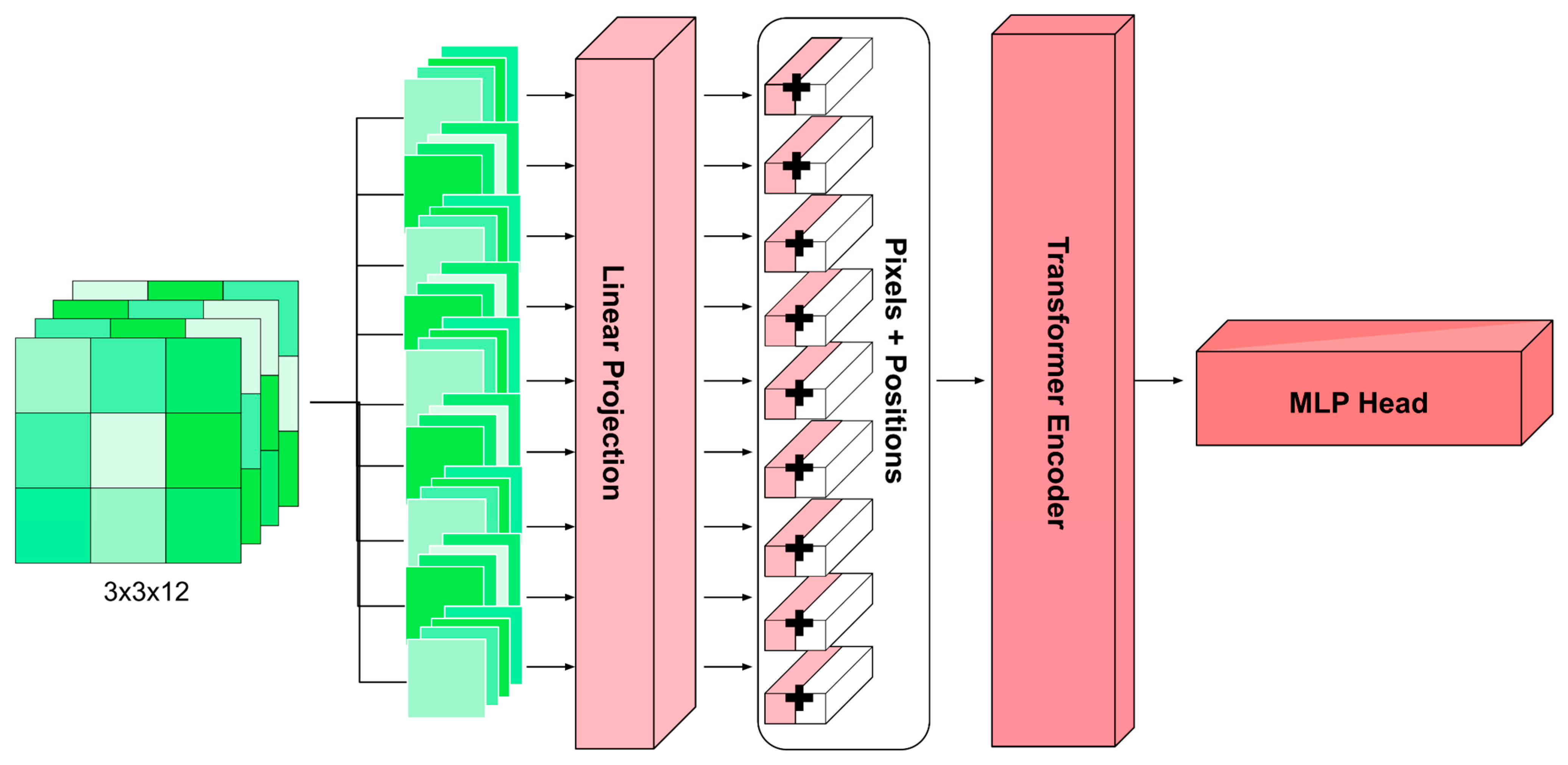
The most complex model we tested was the Vision Transformer [72]. The model processes the input 3 × 3 patch by treating each of the 9 pixels individually and applying positional encoding to each pixel in each layer. Two transformer encoder blocks were used with 8 heads each. The base architecture can be seen in Figure 12. The final classification head of the ViT, an MLP used in this model, had similar parameters to dense layers in the case of the MLP model, with 192 nodes and a ReLU activation function.

2.5. Training and Validation

To fit our datasets to the model architectures, we formed two different input shapes from the same datasets. The MLP requires a flattened input (DSFlat), while the Conv2D and ViT models require a multidimensional input array (DSImg). The flattened input had a batch shape of (512, 108) per iteration, where 108 is the number of the individual values per sample. In the case of the multidimensional input, we used the described shape (512, 12, 3, and 3), representing a 3 × 3-patch context with 12 input features.

The data loaders worked with a batch size of 512, incorporating a shuffle mechanism so that in each epoch the order of the training samples changes. In a GPU environment, we used pinned memory and multiple workers (1–4), allowing data loading to occur in parallel on the CPU. By using this parallelization, the training can be GPU optimized [73].

The classification loss was calculated using weighted focal loss, which is known to improve learning in datasets with a severe class imbalance [74]. The core formulation of focal loss is

$$\mathrm{F}\mathrm{o}\mathrm{c}\mathrm{a}\mathrm{l} \mathrm{l}\mathrm{o}\mathrm{s}\mathrm{s}\left(p_t\right)=-{\alpha }_t(1-p_t{)}^{\gamma }\mathit{log}\left(p_t\right)$$

(2)

where ${\mathrm{p}}_{\mathrm{t}}$ denotes the model’s estimated probability for the correct class, $\gamma$ is the focus parameter (set to 2.0) that down-weights easy samples, and ${\alpha }_t$ is a class-specific weight. These weights, derived using the “Effective Number of Samples” method [75], are defined as follows:

$$a_c=\hspace{1em}{\displaystyle \frac{1-\beta }{1-{\beta }^{n_c}}}, \beta =0.999$$

(3)

where $\beta$ is the smoothing parameter (typically close to 1) and n_c is the number of samples for class c. This formula assigns a higher weight to underrepresented classes, compensating for the class imbalance. The combination of focal loss and the effective number of samples approach enhances the training stability, especially in cases of extreme class imbalances.

During the optimization process, the AdamW algorithm was used. Compared to other adaptive methods, AdamW incorporates an effective weight decay [76]. The initial learning rate was $8\cdot {10}^{-4}$ and the weight decay was $2\cdot {10}^{-5}$; these parameters were chosen to balance fast convergence with protection against overfitting. Weight decay is important especially for models with high parameter numbers, because it helps to restrict excessive parameter growth.

The learning rate was fine-tuned with the “reduce on plateau” parameter. If, at the end of a complete epoch, the macro F1-score did not improve, the learning rate was reduced by a factor of 0.5. This adaptive decay allows the model to make larger parameter updates in the early stages of training and progressively shift to smaller, more precise steps where the learning curve begins to plateau. By using the learning rate decay, the optimization process can converge more smoothly and with higher precision, potentially improving the chances of finding a better (possibly global) minimum. [77].

To ensure the model’s robustness and generalization capability on unseen data, we used k-fold cross-validation, where the number of folds was 4. Each fold had the same sample number ratio across the classes [78]. The number of epochs per fold was set to 50, and an early stopping criterion was also implemented. If the model was unable to reach a better macro F1-score for 10 consecutive epochs, the training was stopped [79]. The best macro F1-score model was chosen for each fold. To ensure reproducibility, the random seed was fixed at 42.

2.6. Evaluation

The stability and robustness were evaluated with a stratified k-fold cross-validation [80]. In each fold, the F1-scores, weighted F1-scores, accuracy, and macro F1-scores were calculated, along with their averages and standard deviations (Supplementary Tables S1–S6). This approach excludes the possibility that one portion of data might distort the results. The macro F1-score-based evaluation is also an effective way to monitor the rare classes’ performance. The validation macro F1-score-based checkpointing ensured that, in every fold, the best model was saved.

The saved folds were then ensembled into one model by averaging the outputs of the models from each fold. This ensembled model was tested on a yet unseen hold-out dataset as the final evaluation of generalizability [81]. The hold-out validation avoids the cross-validation’s optimistic distortion and fits within the remote sensing evaluation practice. The final metrics are based on the hold-out dataset and the ensembled model. To compare the different model architectures, Area Under the Curve (AUC) values and Receiver Operating Characteristic (ROC) curves were calculated (Supplementary Figure S1), which plot the true-positive rate against the false-positive rate [82].

To calibrate the confidence of the probabilistic outputs (i.e., accuracy ratio), a post hoc temperature scaling was also used. This one parameter correction keeps the ranking while it sharpens the SoftMax outputs and decreases the ECE (Expected Calibration Error) [83]. Brier and ECE scores for each fold were also calculated and used as calibration evaluation metrics (Supplementary Tables S1–S6).

$$\mathrm{B}\mathrm{r}\mathrm{i}\mathrm{e}\mathrm{r} = {\displaystyle \frac{1}{N}}{\sum }_{i=1}^N{\sum }_{c=1}^C{\left(p_{i,c}-1\left\{y_i=c\right\}\right)}^2$$

(4)

The Brier formula averages the squared difference between the predicted probability distribution $p$ and the ground truth $y$, where $y$ is represented as a one-hot encoded vector. The averaging is performed over all classes $C$ and over all samples $N$.

$$\mathrm{E}\mathrm{C}\mathrm{E} = {\sum }_{m=1}^M{\displaystyle \frac{\left|B_m\right|}{N}}\left|\mathrm{a}\mathrm{c}\mathrm{c}\left(B_m\right)-\mathrm{c}\mathrm{o}\mathrm{n}\mathrm{f}\left(B_m\right)\right|$$

(5)

The ECE measures the calibration deviation: how well the average confidence of the model matches the actual hit rate at the binned confidence levels. Predictions are grouped into $M$ confidence bins based on their maximum predicted probability, and within each bin, the mean confidence $\mathrm{c}\mathrm{o}\mathrm{n}\mathrm{f}\left(B_m\right)$ is compared to the fraction of correct predictions $\mathrm{a}\mathrm{c}\mathrm{c}\left(B_m\right)$, with weights proportional to the bin sizes ${\displaystyle \frac{\left|B_m\right|}{N}}$.

The logit outputs were calibrated based on the validation dataset; the temperature parameter and the before–-after calibration confusion matrices are included in the Supplementary Material, along with the per-fold metrics and confusion matrices (Supplementary Figures S2–S7).

To compare the models, the Overall Accuracy (OA) was also calculated for each trained model. The OA is the proportion of samples for which the predicted label $y_i^{\prime }$ matches the ground truth label $y_i$. It is computed as the average of the indicator function that is 1 when $y_i^{\prime }=y_i$ and 0 otherwise.

$$\mathrm{O}\mathrm{A} = {\displaystyle \frac{1}{N}}{\sum }_{i=1}^{N}1\left\{y_i^{\prime }=y_i\right\}$$

(6)

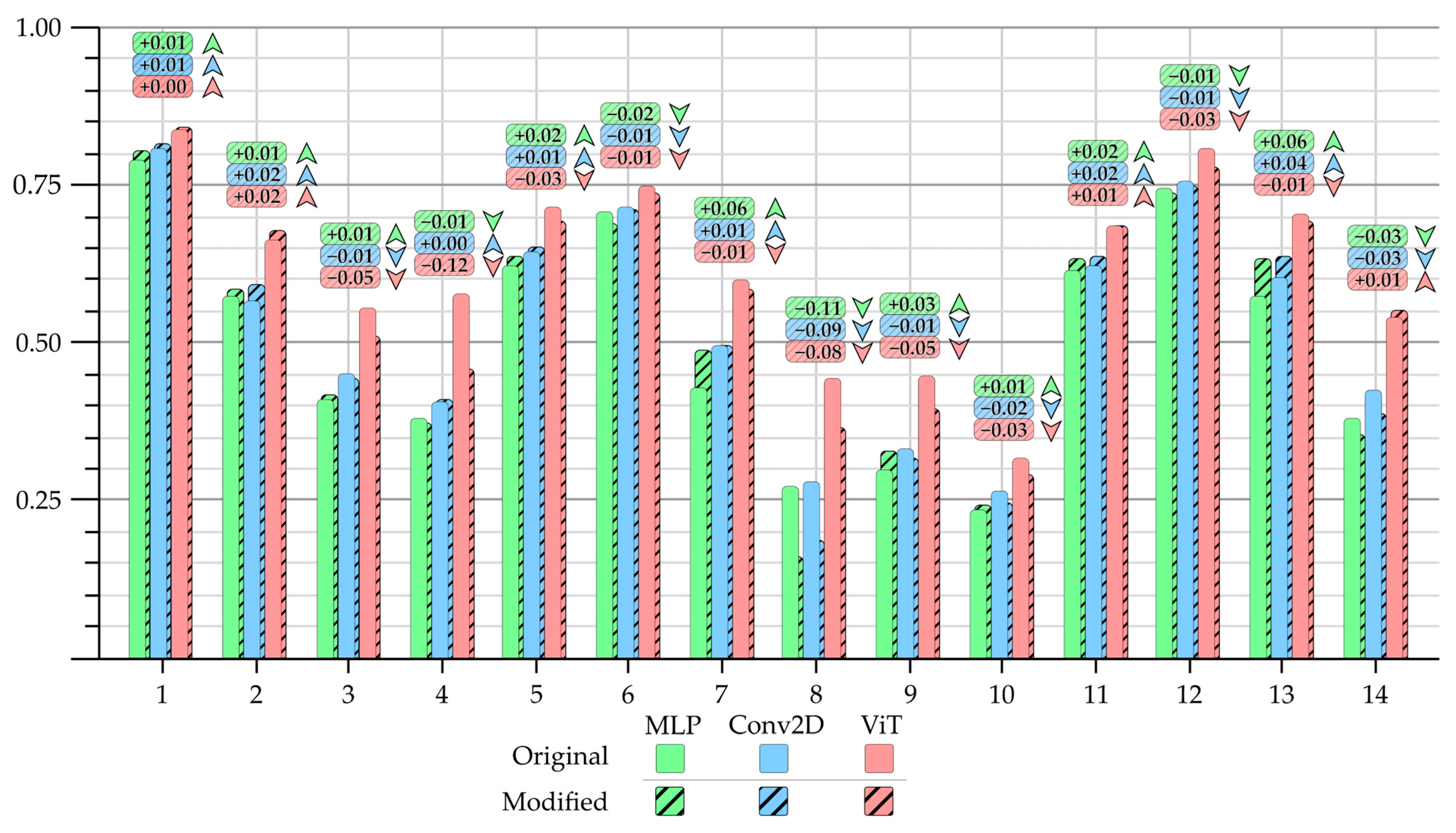
For the class-by-class evaluation, we used the scikit-learn’s classification report function. The AUC differences between the model pairs were analyzed with the DeLong test; the p-values for each class were summarized using Fisher’s method (Supplementary Tables S7 and S8). The report provides the F1-score for each individual class (not aggregated—micro, macro, and weighted; see Supplementary Tables S9–S14), which is the harmonic mean of precision and recall [84]. Precision is the ratio of correctly classified positive items (true positives, TP) to all items classified as positive (TP + false positives, FP). The recall is the ratio of the correctly classified positive items to all relevant items (TP + false negatives, FN). This metric was chosen because the classification models were trained on classes with varying sample sizes, which can lead to misleading statistical results. The F1-score addresses this issue by considering both precision and recall, providing a balanced evaluation.

$${\mathrm{Prec}}_c= {\displaystyle \frac{{\mathrm{TP}}_c}{{\mathrm{TP}}_c+{\mathrm{FP}}_c}}$$

(7)

$${\mathrm{Rec}}_c={\displaystyle \frac{{\mathrm{TP}}_c}{{\mathrm{TP}}_c+{\mathrm{FN}}_c}}$$

(8)

$${\mathrm{F}1}_c={\displaystyle \frac{2{\mathrm{Prec}}_c{\mathrm{Rec}}_c}{{\mathrm{Prec}}_c+{\mathrm{Rec}}_c}}$$

(9)

During the training, and to ensure that the smaller sample number classes also gained enough attention, the macro F1-scores were also calculated and used to evaluate the results.

$$\mathrm{m}\mathrm{a}\mathrm{c}\mathrm{r}\mathrm{o} \mathrm{F}1 = {\displaystyle \frac{1}{C}}{\sum }_{c=1}^C{\mathrm{F}1}_{\mathrm{c}}$$

(10)

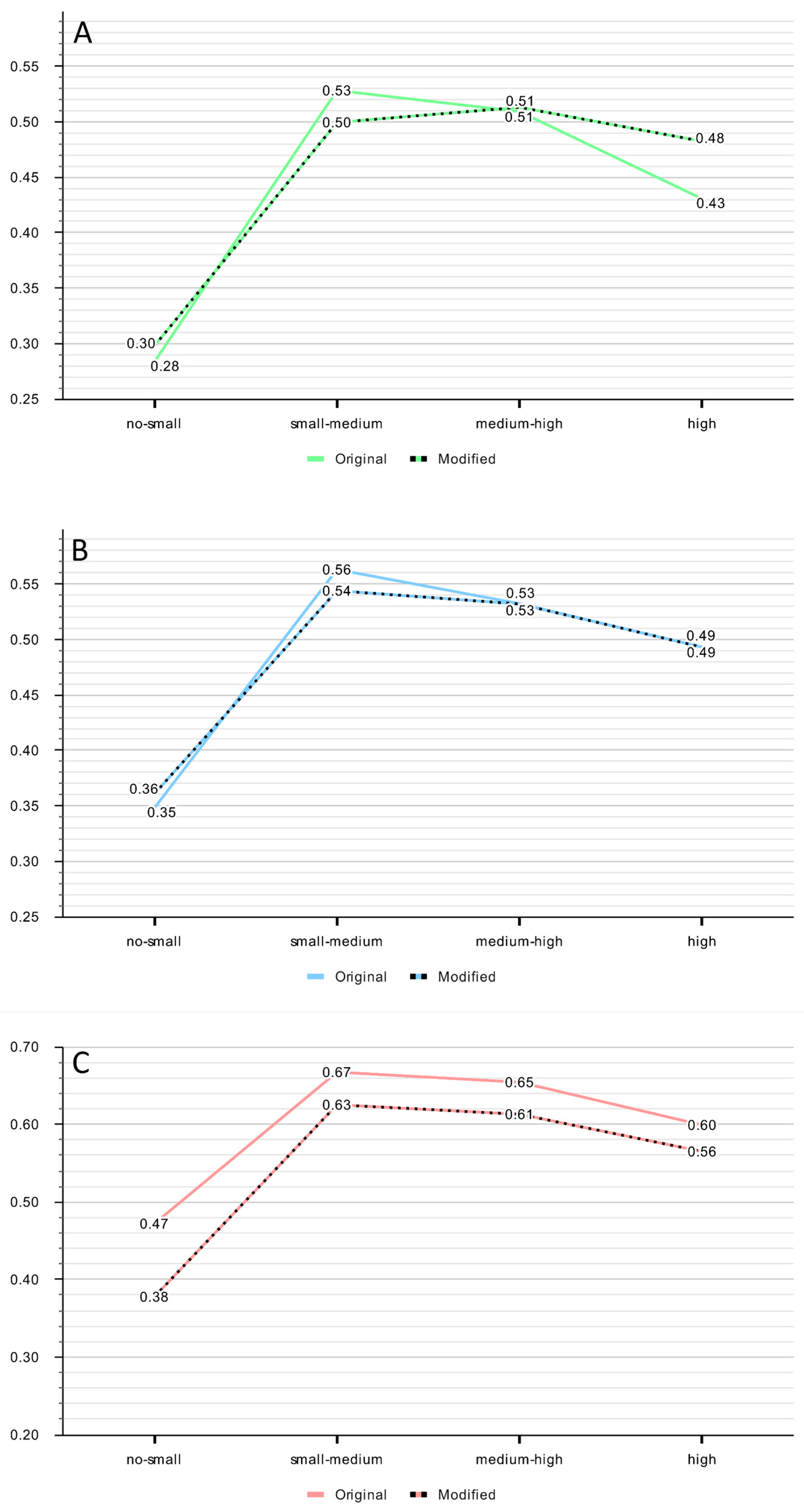
Measuring the effect of vegetation on the predicted raster is challenging. To do this, we used two different metrics to compare the models, both of which use NDVI to represent vegetation. These two methods were the trend of the F1-scores over the defined NDVI classes, while the other metric shows how the accuracy of a class correlates with the vegetation. For the trend analysis, we defined four different NDVI categories (

Table 7. The NDVI categories used for evaluation.

Values	Descriptive Category
0.0–0.2	No–Small Vegetation
0.2–0.4	Small–Medium Vegetation
0.4–0.6	Medium–High Vegetation
0.6–1.0	High Vegetation

).

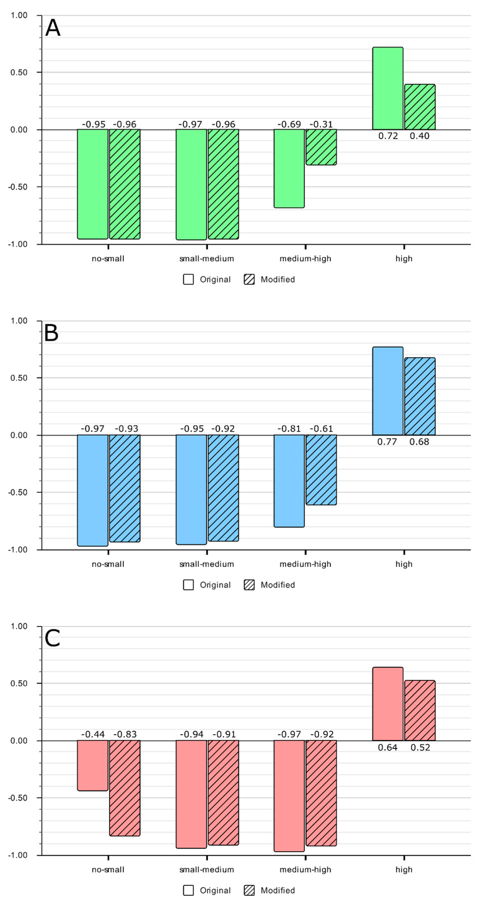
For class-by-class analysis, we used specific correlation-based statistics. An indirect marker NDVI was used as the vegetation descriptor. Four major NDVI groups (major bin) were formulated based on Table 7. Each pixel is classified into a major group $C\left(x\right)$, where $V_i$ is the NDVI value:

$$C\left(i\right)=\left\{\begin{array}{ll}1,& 0\le V_i<0.2,\\ 2,& 0.2\le V_i<0.4,\\ 3,& 0.4\le V_i<0.6,\\ 4,& 0.6\le V_i\le 1.0.\end{array}\right. S_k=\left\{i \right| C\left(i\right)=k\}, n_k=\left|S_k\right|, k=1,\dots ,4.$$

(11)

Every pixel group $S_k$, with $n_k$ number of pixels, is divided into ten subgroups (sub-bins). The separation of sub-bins included the sorting of pixels ${{\{V}_i\}}_{i\in S_k}$ by NDVI and the calculation of deciles (ensuring identical sub-bin $\approx n_k/10$ pixel counts):

$$q_{k,0}<q_{k,1}<\dots <q_{k,10}, q_{k,j}={\mathrm{q}\mathrm{u}\mathrm{a}\mathrm{n}\mathrm{t}\mathrm{i}\mathrm{l}\mathrm{e}}_{j/10}\left(V_i\right|i\in S_k).$$

(12)

The sub-bin level true-positive ${\mathrm{T}\mathrm{P}}_{c,k,j}$, false-positive ${\mathrm{F}\mathrm{P}}_{c,k,j}$, and false-negative ${\mathrm{F}\mathrm{N}}_{c,k,j}$ values served as input for the accuracy measure (macro F1-score), where $P_i$ is the predicted class and $T_i$ is the ground truth:

$${\mathrm{T}\mathrm{P}}_{c,k,j}=\left|\right\{i\in S_{k,j}:P_i=c, T_i=c\left\}\right|,$$

(13)

$${\mathrm{F}\mathrm{P}}_{c,k,j}=\left|\right\{i\in S_{k,j}:P_i=c, T_i\ne c\left\}\right|,$$

(14)

$${\mathrm{F}\mathrm{N}}_{c,k,j}=\left|\right\{i\in S_{k,j}:P_i\ne c, T_i=c\left\}\right|.$$

(15)

Macro F1-score and NDVI averages are formulated for each sub-bin:

$${\mathrm{F}1}_{k,j}^{\mathrm{m}\mathrm{a}\mathrm{c}\mathrm{r}\mathrm{o}}={\displaystyle \frac{1}{\left|C\right|}}{\sum }_{c\in C}{\displaystyle \frac{2{\mathrm{T}\mathrm{P}}_{c,k,j}}{2{\mathrm{T}\mathrm{P}}_{c,k,j}+2{\mathrm{F}\mathrm{P}}_{c,k,j}+2{\mathrm{F}\mathrm{N}}_{c,k,j}}},$$

(16)

$${\overline{V}}_{k,j}={\displaystyle \frac{1}{n_{k,j}}}{\sum }_{i\in S_{k,j}}{V}_i.$$

(17)

The robustness of the K-th major bin is measured by the relationship (${\mu }_{V,k}$, ${\mu }_{F1,k}$) between the ten sub-bins with the Pearson correlation $r_k$:

$${\mu }_{V,k}={\displaystyle \frac{1}{10}}{\sum }_{j=1}^{10}{\overline{V}}_{k,j}, {\mu }_{F1,k}={\displaystyle \frac{1}{10}}{\sum }_{j=1}^{10}{\mathrm{F}1}_{k,j},$$

(18)

$$r_k={\displaystyle \frac{\sum _{j=1}^{10}\left({\overline{V}}_{k,j}-{\mu }_{V,k}\right)\left({\mathrm{F}1}_{k,j}-{\mu }_{\mathrm{F}1,k}\right)}{\sqrt{\sum _{j=1}^{10}{({\overline{V}}_{k,j}-{\mu }_{V,k})}^2}\sqrt{\sum _{j=1}^{10}{({\mathrm{F}1}_{k,j}-{\mu }_{\mathrm{F}1,k})}^2}}}.$$

(19)

The Pearson correlation coefficient $\left(r_k\right)$ is calculated for each of the four main vegetation groups defined in Table 7. Each coefficient resulted from a 10-point measure consisting of the average NDVI and macro F1-score pairs derived from the ten sub-bins within that group. In this analysis, the goal is for the correlation coefficient to be around zero in as many groups as possible. This would indicate that vegetation does not significantly affect classification accuracy, suggesting that the model can be effectively applied in other vegetated areas.

The NDVI–macro F1-score correlation graph shows significant fluctuations. For interpretation, we defined four groups of values (

Table 8. NDVI categories used for evaluation.

Values	Description	Interpretation
(−1)–(−0.5)	As the value of the vegetation index increases, the accuracy decreases significantly.	The classifier relies more on the uncovered lithology’s spectral signature. The vegetation cover decreases accuracy.
(−0.5)–(0)	As the value of the vegetation index increases, the accuracy decreases moderately.	Vegetation impairs classification accuracy to a small to medium extent.
(0)–(0.5)	As the value of the vegetation index increases, the accuracy increases moderately.	Vegetation improves classification accuracy to a small to moderate extent.
(0.5)–(1)	As the value of the vegetation index increases, the accuracy increases significantly.	The classifier relies more on the vegetation’s spectral signature. The vegetation cover improves the accuracy.

). Based on this, the model that performed better is the one whose average correlation does not deviate significantly towards either extreme.

2.7. Hardware Platform and Software Environment

All the tests were conducted in a GPU-assisted environment, using Kaggle Notebooks and Google Colab notebooks, to acquire fast results and ensure reproducibility. The main hardware included an NVIDIA P100 GPU, an Intel Xeon CPU, and 30GB of RAM. The software environment included Python [3.11], PyTorch [2.7.0], CUDA [11.8], and cuDNN [8.x] aligned with CUDA build. Other libraries included Numpy [1.24.x], scikit-learn [1.2], and GDAL [3.x]. During the tests, the seed was fixed (42), the deterministic cuDNN was enabled where it was possible, and mixed precision was used. The models are lightweight and can be trained on average CPUs as well.

3. Results

The results are first presented by showing the performance of the classification models (AUC). The models are tested on both the original data and the data corrected by the FIM. In addition, the classified map produced from the best performing model was also included in the results.

3.1. Macro AUC and Class AUC

The class-level AUC values show that the spectral decorrelation (FIM) caused significant performance gains in several lithological classes. An outstanding example is class 2, where, for the MLP model, the AUC values increased from 0.391 to 0.643; for the Conv2D model, from 0.236 to 0.636; and for the ViT model, from 0.480 to 0.666. The same pattern is observed in the case of class 8, which is the class with the smallest sample count and where the ViT model achieved an almost 0.3 increase with the modified dataset compared to the original. However, class 3 shows the opposite trend, as for that unit, every model’s ability to rank the output dropped significantly (

Table 9. Macro AUC and per-class AUC for each trained model. Values are shown for both the original and FIM-modified datasets.

	Original			Modified
Class	MLP	Conv2D	ViT	MLP	Conv2D	ViT
1	0.434	0.399	0.444	0.437	0.430	0.416
2	0.391	0.236	0.480	0.643	0.636	0.666
3	0.223	0.213	0.330	0.155	0.131	0.188
4	0.710	0.691	0.620	0.637	0.625	0.611
5	0.715	0.644	0.637	0.688	0.602	0.588
6	0.335	0.374	0.460	0.357	0.372	0.397
7	0.588	0.567	0.501	0.588	0.608	0.667
8	0.450	0.615	0.679	0.701	0.850	0.971
9	0.805	0.766	0.712	0.798	0.783	0.553
10	0.677	0.731	0.584	0.560	0.622	0.596
11	0.844	0.835	0.880	0.868	0.872	0.859
12	0.819	0.745	0.825	0.836	0.833	0.806
13	0.701	0.721	0.724	0.665	0.692	0.772
14	0.888	0.940	0.707	0.837	0.824	0.733
Macro AUC	0.613	0.605	0.613	0.626	0.634	0.630

).

Comparing the models on the original dataset, the MLP and ViT show the same Macro-AUC value of 0.613, while Conv2D falls short with 0.605. The FIM shows significant improvement with every model: the largest growth is for Conv2D (from 0.605 to 0.634), while the smallest but still significant growth is produced by the ViT (from 0.613 to 0.630). Overall, the FIM shows a general increase in Macro-AUC scores, while the class-based comparison highlighted the classes that require more attention (Table 9). A visual representation of these results is provided by the ROC-AUC curves (see Supplementary Figure S1). For most classes, the curves for the different models are closely clustered. This visual evidence is supported by the DeLong test p-values (Supplementary Table S2). This indicates that the differences in AUC are not statistically significant, suggesting that the performance variations may have originated more from thresholding and calibration than from fundamental differences in ranking ability.

3.2. Overall Accuracy and Per-Class F1-Score

The Overall Accuracy (OA) values of the models trained on the original dataset ranged between 0.659 and 0.737 (Figure 13). The best-performing model is the ViT, the second best is the Conv2D, and the lowest performing is the MLP model. For the modified dataset, the OA values are between 0.667 and 0.728. There is no change in the performance ranking: the ViT model performed best, Conv2D was second best, and the MLP model performed the lowest. The performance of the MLP shows a small increase in the OA of 0.008, the ViT model’s decreased by 0.009, while the Conv2D model performed almost the same, reaching an OA of 0.682.

The F1-score statistics are mixed, and different results can be observed between the lithological classes, the models, and the two different datasets. The performance metrics show the class-by-class F1-scores and Overall Accuracy scores for all models and both datasets (Figure 14 and Supplementary Table S15). The major lithological type for each class is also included. While the best Overall Accuracy is reached by the ViT in both cases, this result is not consistent across all lithological units.

The per-class F1-scores calculated on the hold-out set are shown in Figure 14. They illustrate how capable the model is at classifying different vegetational environments compared to other models and between different datasets. It was observed that, for both the original and the FIM-modified data, the models performed better on the lithological classes with large spatial extents. In the case of the original dataset, classes 1, 2, 5, 6, 11, 12, and 13 show results consistently above 0.55 for every model. Low-to-moderate performing classes are 3, 4, and 7, while the classes with the worst F1-scores are 8, 9, and 10. The F1-scores of the models trained on the modified dataset are quite similar in terms of the relative performance between classes; the greatest difference is −0.12 for class 4. Changes in per-class F1-scores after FIM modification are also in Figure 14, with exact values provided on labels above the bars. The MLP model shows a decrease ($\delta F1\le -0.02$) in classes 6, 8, 14, keeping the accuracy in classes 1, 2, 3, 4, 10, and 12, while it was able to reach a better F1-score ($\delta F1\ge 0.02$) in classes 5, 7, 9, 11, and 13. The Conv2D model shows decrease in classes 8, 10, and 14, keeping the accuracy in every other class except for classes 2, 11, and 13, where it shows improvement. For the ViT model, the performance decreased compared to the original dataset in classes such as 3, 4, 5, 8, 9, 10, and 12 but remained stable or improved in classes 1, 2, 6, 7, 11, 13, and 14. Indeed, there are classes where the models trained on the FIM-modified dataset outperformed the ones trained on the original dataset. These classes include 2 and 11 for all models and 14 for the ViT model. All models had classes where they generalized better on the modified dataset (Supplementary Table S15). The weighted F1-score considers the class weights, which can explain some score variations, while the performance difference between the more complex models (Conv2D, ViT) is smaller in the case of the modified dataset (Figure 14).

3.3. Calibration

A model’s predictive accuracy does not guarantee that its confidence scores are reliable. To improve this relationship between confidence and accuracy, a post-processing step called temperature scaling was applied to the models’ outputs. The effectiveness of this calibration was measured using the Brier score and the Expected Calibration Error (ECE), where lower values indicate better calibration (see Section 2.5).

After temperature scaling, the Brier and ECE values show improvements across multiple folds, while the OA and macro F1 changed only slightly (when aggregated). The before-and-after calibration confusion matrices and the calculated temperature (T) values are shown in the Supplementary Material (Supplementary Figures S2–S7). This strengthens the model’s probability calibration by confirming a better alignment between model confidence and accuracy.

3.4. Vegetation—F1-Score Trend Charts

To assess model robustness in vegetated terrain, we analyzed the trend of F1-scores across different levels of vegetation density. The hold-out dataset was grouped into four categories based on the NDVI value of each sample (see Table 7 in Section 2.5). The average macro F1-score for each model was then calculated within each of these four NDVI categories.

Considering the vegetation-based F1-score trends, the MLP and Conv2D models show consistency between the original and modified datasets, whereas the ViT shows different dynamics. For the MLP and Conv2D models, the results show mixed trends across the different vegetation densities (Figure 15). In the case of the ViT model, the version trained on the original dataset performs better in every vegetation category.

3.5. Vegetation—F1-Score Correlation

The correlation charts show consistent results, yet there are significant differences between the original and the modified datasets (Figure 16). Each model shows a strong negative correlation in the first three vegetation categories, from no–small to medium–high, except for the ViT model. In the original data, the ViT model shows a less significant negative correlation in the no–small category. In the high vegetation category, the correlation changes to strong positive for all models, though the ViT is less strong with 0.64, while the Conv2D model and the MLP are above 0.7. In the case of the modified dataset, the correlation in the no–small category remains unchanged, except for the ViT, which builds up a stronger negative correlation. The small–medium category shows a less significant decrease with the modified dataset. For the MLP and Conv2D models, the medium–high category is significantly less correlated. The MLP correlation decreases from −0.69 to −0.31 and the Conv2D from −0.81 to −0.61. The ViT also changes but less significantly. In each case, the high vegetation density category shows a significant decrease from the high positive correlation, though the ViT starts from a lower baseline.

3.6. Prediction Map Result

The best performing model is the Vision Transformer trained on the original dataset, so the most accurate predicted map is also produced by this model (Figure 17). Compared to ground truth data, the predicted patterns are mostly well-aligned. Bigger distortions can be observed near the river buffers and at the lithological unit borders (error maps are in Supplementary Figure S8). The shapes of different lithological units are clearly visible, while the borders are less consistent. Key features, like the Densuş-Ciula Formation (classes 5 and 6), are recognized well, as is class 1 (Quaternary), with the largest pixel count. Although the model struggles around the edges, there is little salt-and-pepper noise and a clear distinction between lithological units. Compared to the other classified maps, the best-performing model’s prediction (Figure 17E) provides the clearest lithological units, where the misclassifications are less dominant. Despite its superior overall performance, other models occasionally produced more accurate classifications for specific local areas (e.g., Figure 17D).

4. Discussion

The study had three primary aims. First, to conduct a comparative assessment of the ability of three different machine learning models, including two deep learning-based models, to classify lithological units in a mixed-vegetation-covered study area. Second, to conduct a comparison and assessment of these classifiers on the modified version of the original dataset using FIM, a statistical vegetation suppression method designed for sparsely vegetated areas. Third, to test the effect of vegetation on the Overall Accuracy of each classifier in both datasets. In accordance with the objectives of the study, we aimed to keep the models’ parameter counts as lightweight as possible while achieving the best performance in challenging terrain. To evaluate the results, we utilized three main descriptors: the Overall Accuracy (OA) and AUC values for model comparison and the F1-score statistics across the lithological units of the study area. To measure the effect of vegetation, we used two additional statistics: the average F1-score across vegetation categories and the correlation between vegetation and F1-scores.

4.1. Key Statistics

The Overall Accuracy scores present an improved performance with increasing model complexity. For the original dataset, the MLP performed the lowest, the Conv2D was the second best, and the ViT was the best performer. The gap in OA scores is not large between the MLP and the Conv2D (~1.5–2%), while the difference between the ViT model and the Conv2D is more significant. The same dynamics are present with the modified dataset; the order is the same, although the gap between the MLP and Conv2D shrunk, and the gap is also reduced between the ViT and the Conv2D. The FIM modification led to only minor changes in the OA (as shown on Figure 13): the MLP with the modified dataset shows a small increase in (+0.008), as well as the Conv2D (+0.004), and the ViT model shows a moderate drop with the modified dataset (−0.009).

The class-based F1-score statistics show a mixed performance with recognizable patterns. There are high performing classes (e.g., 1, 2, 5, 6, 7, 11, 12, and 13), with a score higher than 0.55. There are also low performers (e.g., 3, 4, 8, 9, 10, and 14), with a score smaller than 0.5, except for the ViT model in most classes. The correlation between the vegetation index (NDVI) and the F1-score statistics remains consistent for both datasets for the Conv2D model.

4.2. Effect of FIM

As the main statistics show, the models trained on the modified dataset show a drop in Overall Accuracy in the case of ViT. The MLP model struggled less with the modified dataset, as its performance increased in most lithological categories and in the vegetation category-grouped F1-score statistics, while its correlation with NDVI became weaker. The Conv2D model remained resilient to noise suppression; while it showed decreased performance in the small sample size lithological classes, this had a smaller impact on the OA value. The trend chart shows consistent shifts, while the correlation chart shows a step-by-step decrease in negative correlation.

The ViT model did not benefit from the modified dataset in terms of OA, but the model’s response to the FIM-modified data was complex. The F1-score trend chart (Figure 15) shows that, while the general performance curve has a similar shape, the model’s accuracy was consistently lower in the modified dataset across all vegetation categories. The correlation analysis (Figure 16C) helps explain this nuanced behavior.

• In the low-to-medium vegetation areas, the strong negative correlation between the F1-score and vegetation (NDVI) became slightly weaker after FIM modification (e.g., changing from −0.97 to −0.92 in the medium–high category). This suggests that the model relies on the uncovered lithology’s spectral signature, and while the FIM is intended to help the model see the underlying rock, even small vegetation-induced noise can decrease performance.
• In the high vegetation areas, the opposite happens. A strong positive correlation is seen above 0.5 for both datasets, though it also weakened with the FIM (from +0.64 to +0.52). This indicates that, in densely vegetated zones, the model learns to use the vegetation itself as a proxy for the underlying lithology, and the classifier relies more on vegetation (i.e., correlation and accuracy grow in parallelly) to achieve a higher score.

The FIM was able to improve the ranking capabilities (AUC) of the models—particularly in areas with less vegetation cover—while the medium–high NDVI range may have caused distribution and calibration shifts. This helps explain why the AUC improvement does not always translate to better F1/OA values. Class 8 is a good example: the AUC growth is significant, while the F1-score decreased. This could potentially be balanced with threshold optimization, though our calibration was likely influenced by the larger sample size groups. The confusion matrices in the Supplementary Materials, with and without the calibration, support this interpretation.

4.3. Comparisons with Previous Studies

Many studies demonstrate the effectiveness of machine learning and deep learning for lithological mapping [2,4,27,37,41]. However, limited research directly focuses on comparing the performance of various deep learning models on the same dataset with varying vegetation cover. Our research provides a comprehensive evaluation of three models and their suitability for lithology mapping on a study area consisting mostly of sedimentary and metamorphic lithologies. The results with the convolutional network compared to the MLP align with the literature, e.g., [85], as the CNN-based classifiers are much more robust and able to identify local patterns. The superior performance of the Vision Transformer over the convolutional network also aligns with the literature, e.g., [40], as our research also demonstrated its superior performance over the other tested models.

The Forced Invariance Method also performed as we expected: this vegetation suppression method was created for arid and semi-arid areas with low vegetation cover [28]. Our aim was to test if it is applicable in mixed-vegetation areas. In our tests, we found that it does not significantly improve the Overall Accuracy of the models—and can even make models like ViT perform worse—while in some specific classes and with certain models, it was able to increase the accuracy (see MLP, Conv2D—Supplementary Table S15). This is likely because complex models like Vision Transformers learn global patterns [40], and globally shifting the patterns with FIM can negatively affect the ViT’s performance. The global attention mechanism might connect differently distorted regions, causing unstable attention patterns. However, the correlation tests show that in specific vegetation groups, ViT became less sensitive to vegetation after the FIM. It was also found in previous research that, with the use of the FIM, the spectral properties of the uncovered pixels are altered [29]. This effect can also contribute to the worse performance in groups where the correlation values are unchanged.

The different bands of Sentinel-2, each with their own native resolution, were all resampled to 10 m. The 20/60 m bands were resampled using the nearest neighbor method. This approach was carefully considered; it avoids the mixing of spectral information near the edges (unlike bilinear/cubic methods) and does not introduce any synthetic radiometric values. This means that the values of the 20 m and 60 m bands are repeated, and this potential redundancy is handled by the model’s ability to learn from the 3 × 3 contextual window and by the dimensionality reduction from PCA. The PCA contributions also show that the 60 m bands are not among the top three contributors, implicitly gaining less weight.

4.4. Limitations and Possible Improvements

In our tests there were three main limitations: the age and generalized nature of the geological maps, the spatial resolution of the input datasets, and the unbalanced distribution of the lithological units in the study area. The geological maps used for training appear overgeneralized, according to a recent study covering a small part of the area we examined [45]. In addition, although the geological units on the maps were grouped into classes according to their lithology (Table 3), we had no information on the intra-class localization of the diverse lithotypes of the originally more complex groups (e.g., classes 5 and 6). However, as no other, more accurate map of the entire area was available at the start of the current experiment, this problem could not be circumvented. Nevertheless, the spatial resolution of the basic data (10 m) would not have allowed for a detailed, lithology-based classification of geological formations due to their diverse lithotypes. The level of detail of the geological map used was generally consistent with the freely available Sentinel-2 and SRTM DEM data. Although it would have been possible to obtain higher resolution (2.5–3 m) satellite imagery of the land cover, increasing the resolution of the entire dataset would have compromised the lightweight nature of our presented method. If higher resolution DEM and geological data are available for a larger area, it is worth considering re-evaluating the applied machine learning methods to achieve better results, even though the computational requirements would be greater and the methods would no longer be “lightweight”.

The sample sizes were not balanced between the classes, which may have contributed to worse performance in small sample size groups (see F1-score in Figure 14 and Table 3). This limitation resulted from different properties of the study area encountered during the research. First, the spatial distribution of the specific lithological classes is heterogeneous and limited, which is generally characteristic of geological data inherent to their nature: there are formations with a small distribution but characteristic lithological compositions that are unique to the given area, so acquiring such samples from outside the study area was not applicable. Second, synthetic data generation was not applied, because the complex spectral interactions between vegetation cover and lithology were not known with sufficient accuracy. The vegetation correlation analysis supports this decision, highlighting the complexity of the samples. Such data generation would require a detailed vegetation assessment, which is outside the scope of this study.

Although in our study the use of focal loss with effective number-assisted class-weighting improved accuracy in several classes, the improvement achieved in minority groups was not always adequate. Recent studies on the classification of lithological units, which address the problem of unbalanced datasets, are consistent with our findings and often conclude that weighting minority classes does not always lead to satisfactory results [86,87]. Moreover, drastic weighting in the case of highly unbalanced data can reduce the Overall Accuracy [88]. Future studies may aim to overcome this limitation, for example, by adjusting the model’s architecture, testing different loss functions such as softmax loss, e.g., [89], and methods designed to highlight rare classes. When assessing vegetation in context, it is worth considering the use of the Synthetic Minority Oversampling Technique (SMOTE) class balancing method [90], which has already been successfully applied to highlight minority classes in geological classification [91]. Using indirect marker methods for vegetation classification before modifications (e.g., FIM) is also a promising way to improve classification accuracy. By grouping specific regions, the vegetation suppression methods can be focused and weighted based on textural and spectral features.

5. Conclusions

In our research, we evaluated how deep learning classifiers of varying complexity handle lithological mapping in a mixed-vegetation study area. This included an Artificial Neural Network (MLP) as the baseline, a two-dimensional Convolutional Neural Network (Conv2D), and a Vision Transformer (ViT)-based classifier. An important objective was to preserve the lightweight nature of these models, enabling them to work in environments with limited resources while maintaining competitive performance. Our focus was not on maximizing capacity but on achieving a balance between efficiency and accuracy, which is crucial for potential field applications.

We used time-series Sentinel-2 satellite images as a core dataset, augmented with SRTM elevation data. Geological maps from the second half of the 20th century were utilized as ground truth labels for the classifiers. To reduce dataset size and noise, a Principal Component Analysis was used. A 3 × 3 contextual extraction window was used for the pixel-based image analysis.

The main finding of our study is that the best-performing model on this mixed-vegetation landscape is the Vision Transformer. The ViT consistently outperformed the MLP (which showed the poorest results) and the Conv2D (which exhibited a stable but less accurate performance) across various metrics, including Overall Accuracy and AUC, highlighting its capacity to learn more intricate and global patterns from the data.

Furthermore, we investigated the impact of the Forced Invariance Method (FIM). Applying the FIM—a method designed for sparsely vegetated regions—to a medium-to-high vegetation area is unconventional, and our specific aim was to test the applicability and limits of this method outside of its original design context. We found that while FIM did not improve overall performance, and even degraded it for the ViT model, its effects were nuanced. Simpler models (MLP and Conv2D) showed some resilience, and complex models like ViT exhibited unique adaptability, improving performance in some classes, especially on areas with low or high vegetation. This suggests that while the FIM may not be suitable for universal application in mixed-vegetation settings, its altered spectral signatures can be exploited by advanced models.

Despite these promising results, our study faced major limitations: the generalized nature of the available geological maps, the unbalanced distribution of lithological units, and the moderate spatial resolution of the input Sentinel-2 and SRTM data. These factors likely contributed to the lower F1-scores observed in classes with smaller sample sizes. This reflects the inherent trade-off between the lightweight nature of the methods and the challenges posed by the data limitations.

In conclusion, our research underscores the potential of Vision Transformers for robust lithological mapping in complex environments, particularly where vegetation cover varies significantly. While vegetation suppression techniques like the FIM require careful application, advanced models like ViT show a promising ability to adapt to complex spectral data, paving the way for future improvements in automated geological mapping.