Article

A Spatiotemporal Multi-Model Ensemble Framework for Urban Multimodal Traffic Flow Prediction

School of Geomatics and Urban Spatial Informatics, Beijing University of Civil Engineering and Architecture, Beijing 102616, China
*
Author to whom correspondence should be addressed.
ISPRS Int. J. Geo-Inf. 2025, 14(8), 308; https://doi.org/10.3390/ijgi14080308
Submission received: 4 June 2025 / Revised: 4 August 2025 / Accepted: 7 August 2025 / Published: 10 August 2025

Abstract

Urban multimodal travel trajectory prediction is a core challenge in Intelligent Transportation Systems (ITSs). It requires modeling both spatiotemporal dependencies and dynamic interactions among different travel modes such as taxi, bike-sharing, and buses. To address the limitations of existing methods in capturing these diverse trajectory characteristics, we propose a spatiotemporal multi-model ensemble framework, which is an ensemble model called GLEN (GCN and LSTM Ensemble Network). Firstly, the trajectory feature adaptive driven model selection mechanism classifies trajectories into dynamic travel and fixed-route scenarios. Secondly, we use a Graph Convolutional Network (GCN) to capture dynamic travel patterns and Long Short-Term Memory (LSTM) network to model fixed-route patterns. Subsequently the outputs of these models are dynamically weighted, integrated, and fused over a spatiotemporal grid to produce accurate forecasts of urban total traffic flow at multiple future time steps. Finally, experimental validation using Beijing’s Chaoyang district datasets demonstrates that our framework effectively captures spatiotemporal and interactive characteristics between multimodal travel trajectories and outperforms mainstream baselines, thereby offering robust support for urban traffic management and planning.

1. Introduction

The holistic prediction of multimodal travel trajectories constitutes a core component of Intelligent Transportation Systems (ITSs), offering critical scientific support for urban traffic management and planning [1,2,3]. People often use bicycles, motor vehicles and other models of travel in the real urban traffic network. However, the coexistence of diverse transportation modes in urban systems makes it difficult to integrate and analyze all modes effectively for accurately predicting overall urban traffic patterns in traffic flow prediction research [4,5]. Currently, urban traffic flow prediction tasks typically exhibit the following characteristics:
(1)
Dynamic interaction among multimodal travel trajectories. In urban traffic networks, different modes of transportation (such as bike-sharing, taxis, and buses) not only exhibit strong spatiotemporal characteristics, but also generate movement trajectories that demonstrate complex interaction patterns across both spatial and temporal dimensions [6,7].
(2)
Multimodal travel trajectory features. The spatiotemporal characteristics of urban multimodal travel trajectories stem from the interaction dependencies and latent correlations among different travel modes across space and time [8]. Based on the different trajectory features, it is necessary to consider the trajectory characteristics of different transportation modes (e.g., bike-sharing, taxis, and buses) for flow prediction.
(3)
Multi-model ensemble. Travel trajectories have significant heterogeneity in spatial and temporal dimensions, and different travel characteristics have different requirements for model adaptation [9]. By integrating the features predicted by each model with the multi-model ensemble strategy, the overall traffic flow of multimodal travel in the city can be well reflected.
Despite recent advances, existing studies exhibit two major limitations: First, most models focus on single mode predictions, neglecting the mutual influence across transportation modes, thus failing to reflect the collaborative dynamics of multimodal urban systems. Second, current methods often apply uniform modeling strategies, which overlook the distinct characteristics of different trajectory types, such as the randomness of taxis versus the periodicity of buses.
To address these limitations, this study combines trajectory interaction modeling with multi-model ensemble learning, establishes a trajectory feature adaptive model selection mechanism to distinguish dynamic (such as taxis) and fixed-route (such as buses) travel modes, and constructs an ensemble learning framework. The heterogeneous outputs of these models are integrated through dynamic weights to achieve comprehensive urban traffic flow prediction. The main contributions of this work are as follows:
  • We propose a feature-adaptive selection mechanism to match travel scenarios with appropriate predictive models (Graph Convolutional Network (GCN) for dynamic and Long Short-Term Memory (LSTM) for fixed-route modes). This approach generates heterogeneous feature representations that serve as inputs for the subsequent multi-model ensemble process.
  • We introduce a dynamic weighted integration strategy, and use the traffic fusion calculation method to generate comprehensive traffic flow prediction results through the output of the spatiotemporal grid mapping fusion model.
  • Extensive experiments on real datasets demonstrate that the proposed method is significantly superior to existing methods in terms of prediction accuracy.

2. Related Works

With the continuous development of traffic trajectory prediction research, methods have evolved from traditional statistical models to machine learning, and further to deep learning and ensemble learning. Initially, traditional prediction methods were mainly based on statistical theories. Smith et al. [10] proposed the Historical Average Model (HAM), which uses historical average data as the prediction result, but it suffers from low prediction accuracy. Time series models, such as Autoregressive Integrated Moving Average (ARIMA) [11] and its variants [12], and an ARIMA variant model that predicts by analyzing the relationship between current and historical data proposed Lee et al. [13], consider the seasonality and trends of the data. However, these methods are time series-based and fail to capture spatial structural features.
Subsequently, traffic prediction models based on machine learning alleviated the shortcomings of traditional models. Davis et al. [14] were the first to apply the K Nearest Neighbors (KNNs) algorithm to traffic trajectory prediction, but this model relies heavily on distance metrics and lacks interpretability. Other methods, such as Lefèvre et al. [15] using Bayesian inference, Hu et al. [16] using Support Vector Machines (SVMs) method, and Firl et al. [17] using Hidden Markov Models (HMMs) for traffic trajectory prediction, all depend heavily on empirical features and struggle to capture the complex nonlinear patterns of traffic trajectories.
Deep learning models have gained widespread attention for their advantages in capturing nonlinear patterns [18]. For instance, Jia et al. [19] proposed Deep Belief Networks (DBN) and Lv et al. [20] proposed Stacked Autoencoder Networks (SAEs) for travel trajectory prediction. However, these methods typically treat trajectory information at each time point independently and fail to fully exploit the dependencies within the time series. To address this, researchers have proposed sequence prediction-based Recurrent Neural Networks (RNNs), such as the DCRNN framework proposed by Li et al. [6], which captures spatial correlations through bidirectional random walks on graphs and utilizes an encoder–decoder architecture to capture temporal dependencies, although the gradient vanishing problem still exists in long-sequence modeling. In response, researchers turned to LSTM [21] and Transformers [22]. Ma et al. [23] used LSTM combined with sensor data from vehicles and trajectory data to predict future trajectories. Liu et al. [22] used a stacked Transformer to aggregate fixed-trajectory context information and used trajectory generators and selectors to decode each feature for prediction. Zhang et al. [24] proposed using Gated Recurrent Units (GRUs) for traffic trajectory prediction, effectively addressing the bottleneck of short-term memory networks and extracting long-term dependencies. While these models effectively capture temporal features of travel trajectories, spatial features are also considered crucial for prediction accuracy.
To this end, ensemble methods that select appropriate models for processing temporal and spatial features separately have been developed. Liu et al. [25] improved prediction accuracy by introducing a CNN to extract spatial information and combining it with LSTM. However, since the Convolutional Neural Network (CNN) [26,27] is based on a regular grid structure, it faces inherent limitations in dealing with complex graph topological relationships in the traffic network (such as the connectivity of intersections and the non-uniform distribution of road sections), and cannot capture the spatial characteristics of traffic trajectories inherently. In this regard, a Graph Convolutional Network (GCN) handle complex interaction network relationships well [28,29]. Zhao et al. [30] proposed T-GCN, which integrates the GCN and GRU models to better handle spatiotemporal dependencies in traffic networks. Considering the impact of external conditions, Liu et al. [31] proposed an STAEformer model, significantly improving the prediction capability of traffic trajectory. Patara T et al. [32] introduces the Spatiotemporal Graph Neural Controlled Differential Equation (STG-NCDE) method, which combines temporal and spatial processing using neural controlled differential equations to achieve superior accuracy in traffic forecasting compared to 20 baseline models. Choi et al. [33] proposes the DF-TAR network, which combines dangerous driving statistics with external environmental factors to improve traffic accident risk prediction accuracy compared to the benchmark model. Wang et al. [34] developed an integrated prediction model based on an attentional mechanism and a 1DCNN-LSTM network, which combines the strengths of two models with excellent prediction results but does not consider the interactions between their transportation modes. Wen et al. [35] proposed a decomposition dynamic graph convolutional recurrent network (DDGCRN) for traffic flow prediction. This method combines dynamic graph generation based on an RNN, which can capture the spatial and temporal characteristics of time changes, and uses data-driven modeling to improve prediction performance.
In summary, existing trajectory flow prediction methods face two major limitations. First, most current approaches focus on isolated analysis of a single transportation mode, lacking a unified modeling framework capable of capturing the coordinated dynamics of a multimodal urban transportation system. This deficiency hampers the comprehensive simulation and forecasting of traffic flows across the entire road network. Second, there exist significant differences in trajectory characteristics across various travel scenarios, for instance, the strong periodicity of fixed-route traffic versus the randomness of dynamic travel modes such as taxis and bike-sharing. However, many existing studies adopt homogeneous modeling strategies, which fail to effectively accommodate both the sequential regularities of public transit and the dynamic interaction patterns of flexible travel modes.
To address these challenges, this paper proposes an ensemble learning framework tailored for multimodal transportation networks, aiming to overcome the limitations of existing methods in modeling intermodal interactions and scenario heterogeneity. Specifically, the proposed approach employs a graph-based model to capture the dynamic spatiotemporal interaction patterns of free-flow traffic modes (e.g., taxis and bike-sharing), and utilizes a temporal-sequence model to characterize the sequential operating features of fixed-route traffic modes (e.g., buses and subways). Building upon this foundation, a multi-model ensemble mechanism is designed to adaptively coordinate the predictions from different models based on travel scenario characteristics. Through dynamic weight allocation, the framework fuses model outputs to construct a unified traffic prediction method that effectively reflects the collaborative dynamics of diverse travel modes within the urban system.

3. Basic Definitions

3.1. Trajectory Flow Prediction Problem

The multimodal trajectory prediction problem can be abstracted as a sequence generation problem. In real traffic scenarios, for each type of vehicle i i = 1,2 n , its position at time t ( t = 1,2 , , t o b s ) is represented by the coordinates p i t = x i t , y i t . The historical trajectories of multimodal of transportation are given as X = [ p i 1 , p i 2 , , p i t o b s ] . In prediction, the interaction between different travel modes is considered to influence the target vehicle’s trajectory. This means that the factors affecting the future trajectory of the target vehicle are not limited to its historical trajectory data but also include the trajectory information of surrounding travel modes, S = [ s i 1 , s i 2 , , s i t o b s ] . After training the model, the output is the future coordinate sequence of the target vehicle from time t o b s + 1 to t p r e d , as shown in the following Equation (1):
Y = p i t o b s + 1 , p i t o b s + 2 , , p i t o b s + t p r e d = f X , S
where f   is the prediction model. After this, the predicted trajectories are mapped to a spatiotemporal grid Q as follows (2):
Q = m = 1 t p r e d I ( Δ x p i , t o b s + n , Δ y p i , t o b s + n , Δ t n , k )
where I is the mesh assignment indicator function, and k is the type of travel.

3.2. Spatiotemporal Coupling Across Trajectory Modalities

In urban transportation systems, the trajectory behaviors of different travel modes form dynamic interaction relationships through spatiotemporal coupling and correlation mechanisms [36,37]. For dynamic travel scenarios (e.g., taxis and bike-sharing), as illustrated in Figure 1, trajectory interactions can be modeled using a graph structure G = V , E , A . Here, the node set V represents the feature vector set of complete vehicle trajectories; each edge in the edge set E captures the interactive influence between two trajectories. The adjacency matrix A encodes the pairwise relationships, where each element A i j denotes the OD (origin–destination) distance between the trajectories of vehicle i and vehicle j . The edge weight is defined by the following function (3):
A i j = f ( O i j , T i j )
where O i j represents the OD matrix, T i j denotes temporal factors, and f is a function used to adjust the edge weight. For fixed-route scenarios (e.g., buses), trajectory characteristics are primarily modeled by a spatiotemporal correlation function C ( t ) , defined as follows (4):
C ( t ) = F ( T ( t ) , Y ( t ) )
where F is a modeling function, T ( t ) captures the periodic operating patterns, and Y ( t ) maps the spatial distribution of trajectory points. This coupling mechanism jointly analyzes the stochastic interactive nature of free-flow traffic and the periodic regularity of fixed-route transportation. It serves as a foundational principle in most trajectory prediction and modeling studies.

3.3. Multi-Model Ensemble

To solve the complexity problem of multimodal traffic trajectory prediction, this paper proposes an ensemble method based on parallel network model fusion [38]. This method captures dynamic interaction features and fixed timing rules by combining different network models to differentiate modeling units. For N independent models M i ( i 1,2 , , n ) . The model M i is trained using the given trajectory dataset D = [ ( x 1 , y 1 ) , ( x 2 , y 2 ) , , ( x m , y m ) ] , and its model parameters θ i are determined by the following Equation (5):
θ i = argmin θ i L ( M i ( x ) , y )
where L denotes the model loss function. After each parallel model M i is trained, it independently generates the predicted result   y ^ i = M i ( x ) . The final integrated prediction value y ^ is generated by dynamic weighted fusion as (6):
y ^ = i = 1 N w i y i ^ i = 1 N w i
where w i represents the weight of the model.

4. Data and Methods

4.1. Studied Area and Dataset

The proposed GLEN framework achieves accurate trajectory prediction across multiple modes of transportation by matching the most suitable model (GCN or LSTM) with each travel type, and improves prediction performance through dynamic ensemble learning, that is, considering real traffic constraints while integrating heterogeneous model outputs.
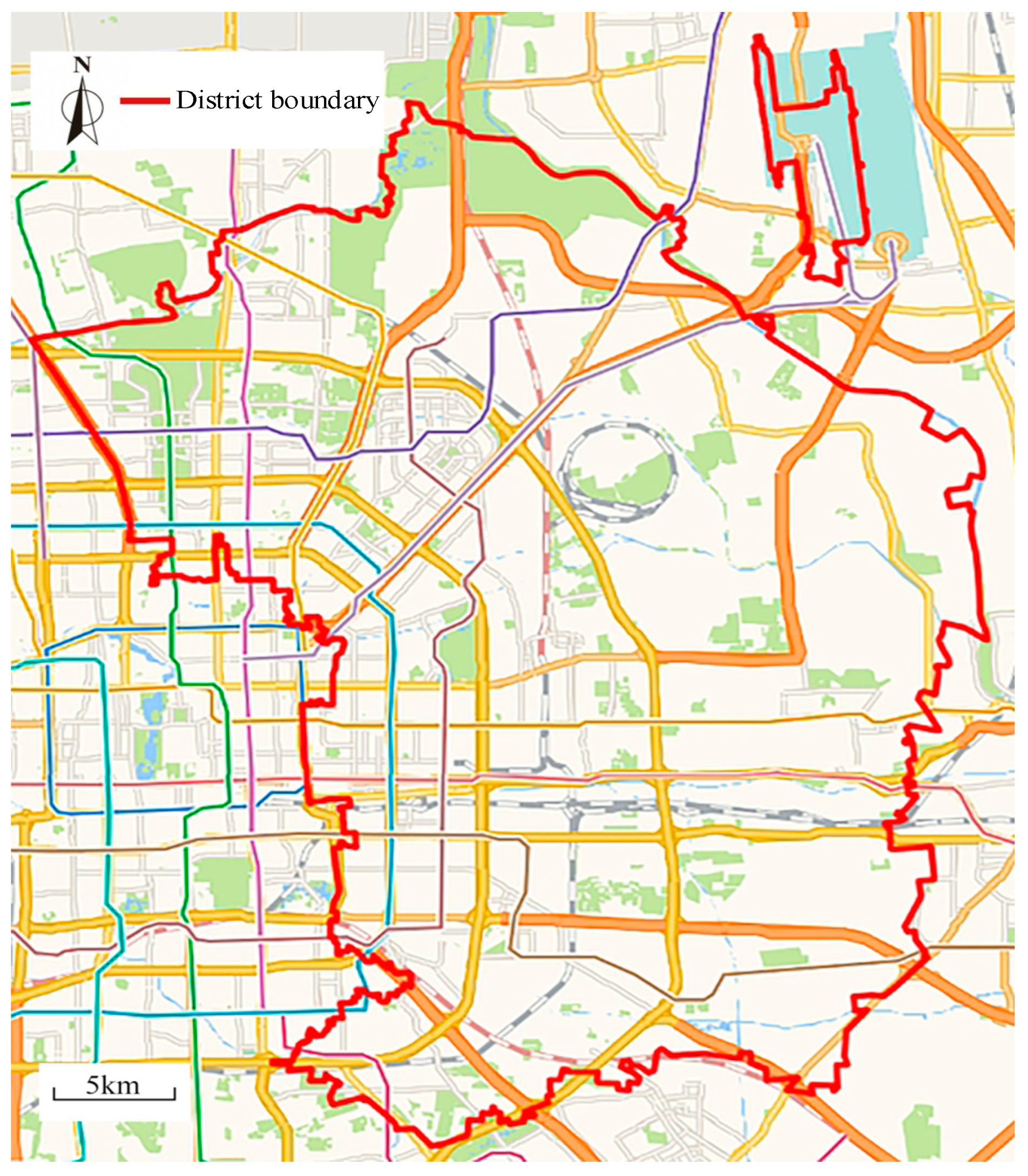
To validate the effectiveness of the proposed method across multimodal travel mode scenarios, we selected Beijing’s Chaoyang district as our study area (with an area of 470.8 square kilometers and a resident population of 3.452 million), as shown in Figure 2. It includes complex traffic environments, from the Central Business District to the Olympic zone, and exhibits typical characteristics of a multimodal transportation system.
We use real traffic trajectory data from this region, including taxi data, bike-sharing data, and bus data, to conduct our experiments. The dataset comprehensively captures the spatiotemporal patterns of various modes of travel within the entire region, and Table 1 presents a sample of the collected trajectory data.
The taxi trajectory dataset contains the full-day trajectory data of taxis in Beijing on 27 May 2019. The bus trajectory dataset covers the bus card swipe trajectory data in Beijing on 27 May 2019. The bike-sharing trajectory dataset comes from the Mobike Algorithm Challenge and includes the full day trajectory data of shared bicycles in Beijing on 27 May 2017. Taking the Chaoyang District of Beijing as an example, we selected trajectory data from the same area and extracted 5246 complete real trajectories for each type of trajectory data. By calculating the adjacency matrix based on the interaction distance between trajectories and constructing a trajectory interaction graph, we describe the interaction between different modes of transportation. Then, based on the time series, we construct a spatiotemporal feature matrix, where the rows are indexed by trajectories and the columns are indexed by timestamps. For missing values in the trajectory data, we use linear interpolation [39] to fill in the gaps, ensuring the completeness of the data.
Although the time span of the bike-sharing data does not exactly match that of the taxi and bus trajectory data, by selecting the same day from the same quarter for analysis, we effectively minimized the interference of seasonal factors and ensured a certain level of consistency in the data.

4.2. Overall Spatiotemporal Multi-Model Framework

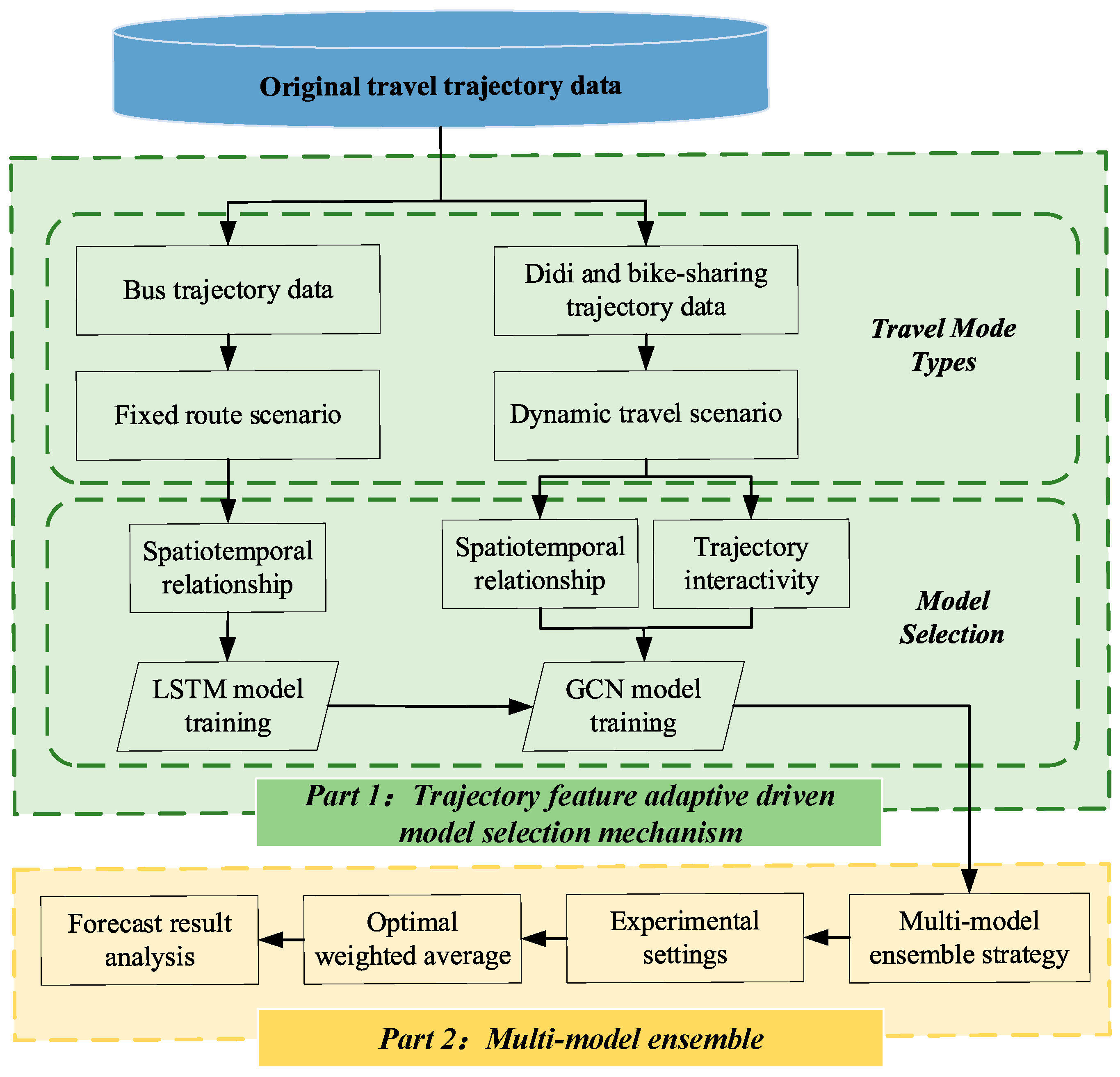
This paper proposes a research framework for multi-model ensemble, which is GLEN (GCN and LSTM Ensemble Network). The overall framework is illustrated in Figure 3, which is mainly composed of two parts: the trajectory feature adaptive driven model selection mechanism and the multi-model ensemble. Firstly, the trajectory feature adaptive driven model selection mechanism divides citizens’ travel into two distinct scenarios—dynamic travel and fixed-route travel. The original trajectory data is preprocessed into 15 min interval sequences to form the input sequences. For flexible dynamic travel modes such as taxis and bike-sharing, GCN is used to model their spatiotemporal correlation and trajectory interaction characteristics. For fixed-route travel modes such as buses, LSTM is used to model their time series and trajectory distribution characteristics. Based on the dynamic differences in different travel modes, a multi-model architecture is designed to model these scenarios separately. Secondly, after each model is independently trained, transitioning into the multi-model ensemble phase. This strategy involves weighting and averaging the prediction results of the GCN and LSTM models and combining the strengths of each model to generate the final trajectory prediction [40]. The weights can be dynamically adjusted based on the performance of each model, ensuring the stability of the prediction results.
To validate the proposed framework in an urban transportation context, we selected Chaoyang District of Beijing as the case study area. This region exhibits high population density, diverse travel patterns, and a complex multimodal transportation system including taxis, bike-sharing, and buses. These characteristics make it an ideal test to assess the effectiveness of a trajectory-based ensemble model framework that captures both spatial heterogeneity and intermodal interactions.

4.3. Trajectory Feature Adaptive Driven Model Selection Mechanism

4.3.1. Dynamic Trajectory Feature Scenario

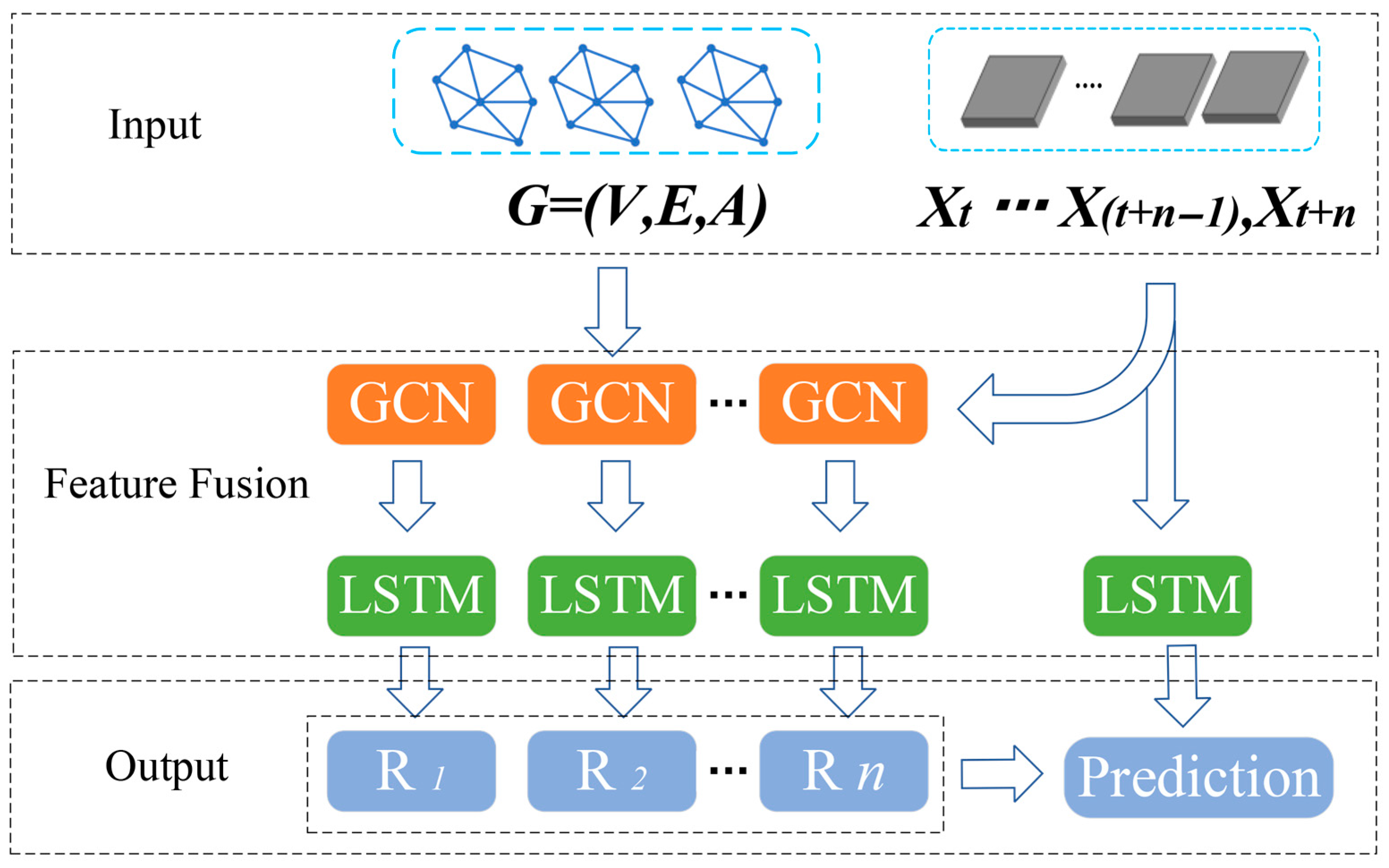
For dynamic travel modes such as taxis and bike-sharing, their trajectory patterns are not constrained by rigid scheduling rules, making them inherently more flexible, random, and thus exhibit stronger interaction among trajectories. To capture these spatial interactions, we employ a GCN-based prediction framework; GCN is a deep learning model designed to operate on graph-structured data, learning local and global patterns in data, making them highly effective for tasks like spatial interaction modeling. Using an OD distance threshold to determine whether pairs of trajectories exhibit high spatial proximity, which serves as the basis for constructing the interaction graph. Specifically, a predictive architecture is established for these flexible modes, as illustrated in Figure 4.
To capture the interaction information between vehicle trajectories, we first define the weight matrix W based on the similarity between vehicle trajectories; the spatial distance threshold constraint is introduced, and the adjacency matrix A (the edge weight in the non-threshold range is set to 0) is calculated to characterize the interaction intensity between dynamic traffic objects. After obtaining the adjacency matrix A , the vehicle trajectory information is propagated over the graph structure using a GCN. At the same time, let the hidden state of each vehicle be h t , where t [ 1,2 , , n ] . The hidden state h t already contains the spatiotemporal feature information of each vehicle. These hidden states form the matrix X , with dimensions X × d h , where d h is the dimension of the hidden state. The matrix X is input into the LSTM to extract temporal features and hidden time states. Finally, the output feature tensor from each layer can be expressed by Equation (7).
R ( l + 1 ) = σ ( D ^ 1 2 A ^ D ^ 1 2 R ( l ) W ( l ) )
where σ denotes the activation function, and A ^ =   A +   I , D ^ represents the degree matrix of A ^ . R ( l ) is the matrix formed by concatenating all node vectors (trajectory interaction) at layer l , and W ( l ) is the weight matrix for the GCN at layer l . Through multilayer GCN operations, the final output feature R represents the interaction features between vehicle trajectories. This will be concatenated with the time features output from the LSTM to generate future trajectories.

4.3.2. Fixed-Route Trajectory Feature Scenario

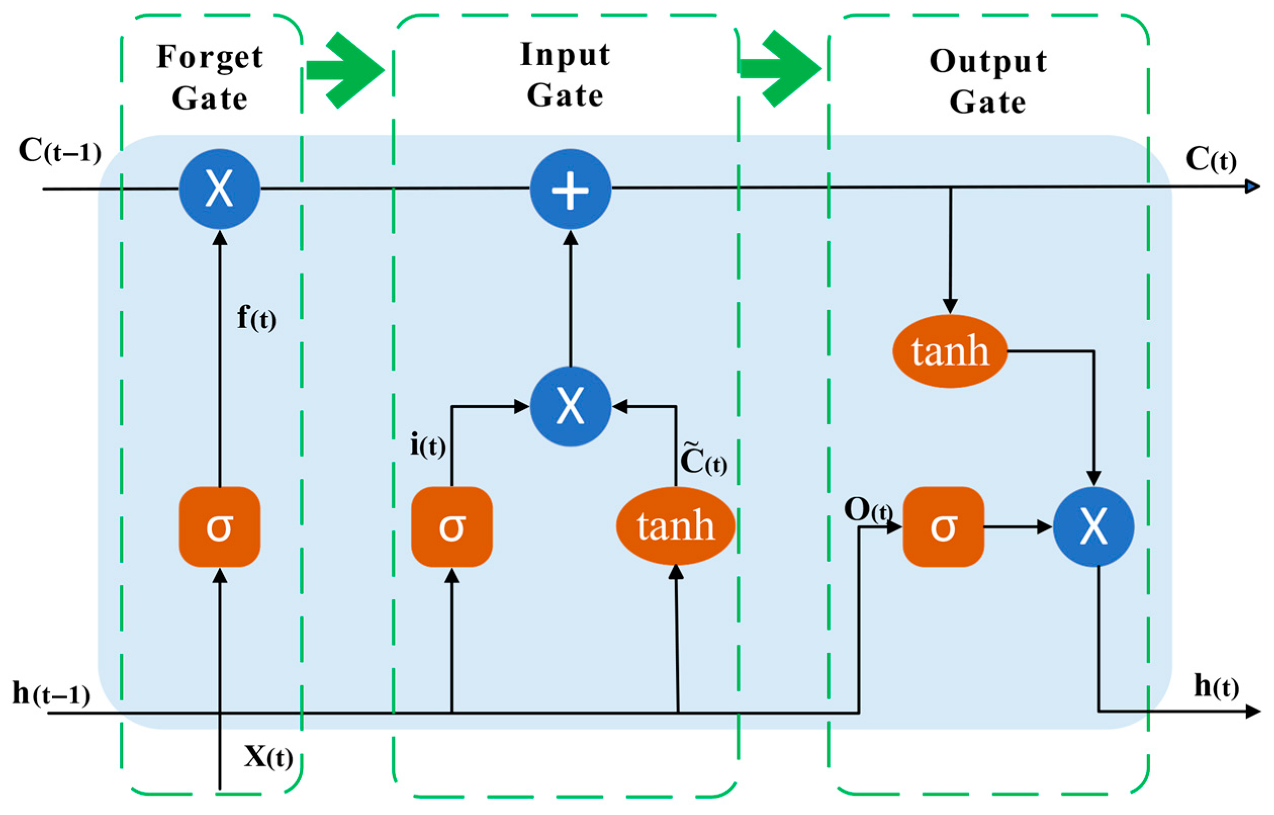
For fixed-route travel modes such as buses, their trajectory patterns are constrained by predefined routes, exhibiting clear periodicity and stable spatiotemporal dependencies. This periodicity is mainly driven by external factors such as daily travel time, route timetables, and traffic conditions. Spatiotemporal dependence refers to the relationship between trajectory data at different time and location points, which are located along the predetermined route. These feature patterns naturally guide the selection of LSTM as a modeling method, because it can learn the periodic characteristics and time dependence of bus routes in sequence data, and solve the problem of gradient disappearance. The prediction process based on this model is shown in Figure 5, where LSTM is used to predict future traffic trajectories based on historical trajectory data. The model first analyses the time pattern and spatial distribution of bus trajectories, and identifies repeated patterns that change over time. Then, it predicts the future state of the bus trajectory based on these models, to more accurately understand the information transmission under different conditions.
The model gated mechanisms to dynamically capture periodic patterns in vehicle operations as well as spatial distribution characteristics. The hidden state of a vehicle at time step t , denoted as h t , is computed according to the following Equations (8)–(13):
i ( t ) = σ ( W i [ h ( t 1 ) , x ( t ) ] + b i )
C ~ ( t ) = t a n h W c h t 1 , x ( t ) + b c
f ( t ) = σ W f h t 1 , x ( t ) + b f
C ( t ) = f t C ( t 1 ) + i ( t ) C ~ ( t )
o ( t ) = σ ( W 0 [ h ( t 1 ) , x ( t ) ] + b 0 )
h ( t ) = o ( t ) t a n h C ( t )
where i ( t ) , f ( t ) , and o ( t ) represent the input gate, forget gate, and output gate of the LSTM, respectively. [ h ( t 1 ) , x ( t ) ] represents the concatenation of the previous hidden state h ( t 1 ) and the current input x ( t ) . C ( t 1 ) and   C ( t ) are the cell states at time t 1 and t , respectively, while C ~ ( t ) represents the candidate cell state. W denotes the weights and b represents the learnable parameters. σ and t a n h are the activation functions.

4.4. Multi-Model Ensemble

4.4.1. Dynamic Weights for the Multi-Model Ensemble Strategy

In this study, a feature adaptive driven model selection mechanism is employed to choose the appropriate prediction model based on different types of trajectory features. Specifically, the GCN prediction model is used for taxi and bike-sharing trajectories, while the LSTM prediction model is used for bus trajectories. For the prediction results, a weighted averaging method is used for multi-model ensemble [41], as shown in the following Equation (14):
S c o r e = i = 1 N   w i s i N
where N is the number of model results, ω i is the weight corresponding to the prediction result of model i , and s i is the corresponding prediction result. The weights must satisfy the conditions: ω i 0   a n d   i = 1 N ω i = 1 . To find the optimal combination of weights, all possible combinations of weights were evaluated by means of a systematic search, considering that the weights must satisfy the condition of normalization, i.e., the range of each weight value is from 0.00 to 1.00, varying in steps of 0.01 and keeping the sum of their weights to 1.

4.4.2. Flow Fusion Computation

To enable collaborative analysis of prediction results from both the dynamic travel and fixed-route scenarios, we propose a fusion method based on spatiotemporal gridding and physical constraints. Firstly, the heterogeneous prediction results of GCN and LSTM are uniformly mapped to the spatiotemporal grid of urban road network. Each grid cell corresponds to a specific road segment at a given time step. The fused traffic flow at each grid cell ( i , t ) is computed as (15)
y ^ ( i , t ) = α ( i , t ) Φ G C N ( X d y n ) + ( 1 α i , t ) Φ L S T M ( X f i x )
where α ( i , t )   is a dynamic weighting factor, Φ G C N and Φ L S T M denote the prediction results from the GCN and LSTM models, X d y n and X f i x are the input features corresponding to dynamic and fixed-route travel modes. To ensure the fused traffic flow aligns with physical road constraints, a road capacity constraint is applied as (16):
y ^ ( i , t ) C m a x
where C m a x denotes the maximum traffic capacity of the corresponding road segment. This constraint guarantees that the resulting traffic flow predictions remain consistent with the practical load bearing limits of the transportation infrastructure, thereby yielding reliable flow estimates for each road segment and time step.

5. Results

5.1. Accuracy Evaluation Metrics of the Model GLEN

To quantify the performance of the multimodal trajectory prediction model, this paper adopts the root mean square error (RMSE) and the mean absolute error (MAE) as the core evaluation metrics (e.g., Equations (17) and (18)). RMSE evaluates the overall discrepancy between the predicted values and the actual values by taking the square root of the average squared differences. In contrast, MAE evaluates the robustness of prediction errors by averaging the absolute differences, mitigating the influence of error direction on the result.
R M E S = 1 n t = 1 n   y t y ^ t 2 1 2
M A E = i = 1 n   y t y ^ t n
where n denotes the number of samples, y t represents the actual trajectory value, and y ^ t is the corresponding prediction.

5.2. Parameter Settings of the Prediction Model GLEN

During the model training process, the input data is normalized to the range [0, 1]. The dataset is divided into training, validation, and test sets with a ratio of 8:1:1, where 80% of the data is used for training, 10% for validation, and the remaining 10% for testing. The Adam optimizer is used to train the two different models, with a learning rate set to 0.001, a batch size of 64, and a training set proportion of 0.8. Other hyperparameters are determined experimentally.
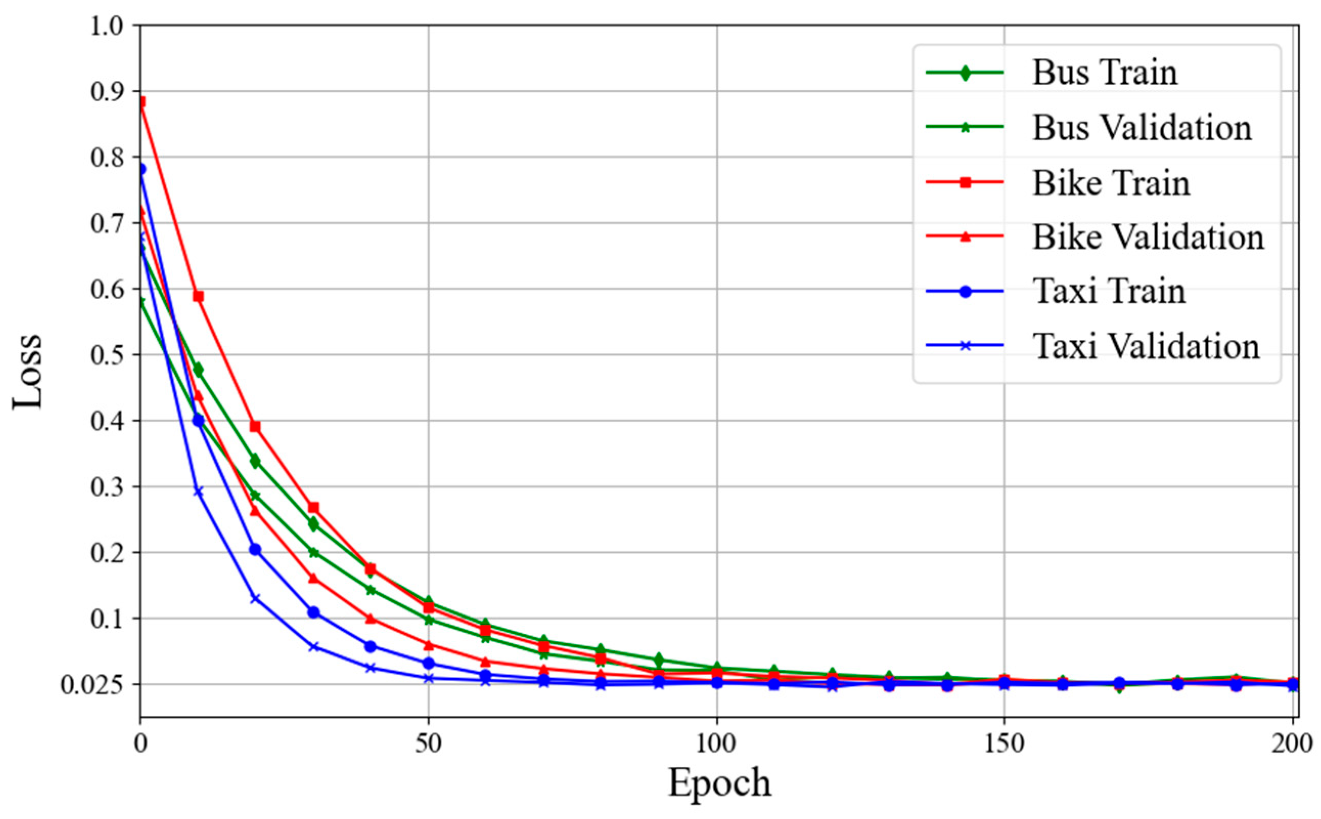
During training, the training EPOCH for both models is set to 200. The training results are shown in Figure 6. The taxi prediction model stabilizes after 80 EPOCHs, while the prediction models for shared bicycles and buses gradually converge after 120 EPOCHs. The loss for these three models decreases continuously in both the training and validation sets as EPOCH increases and approaches convergence, indicating that the model’s prediction performance has met expectations.
In addition, the number of hidden units is a key parameter that affects prediction accuracy. We selected the optimal value by comparing the model prediction results with different numbers of hidden units.
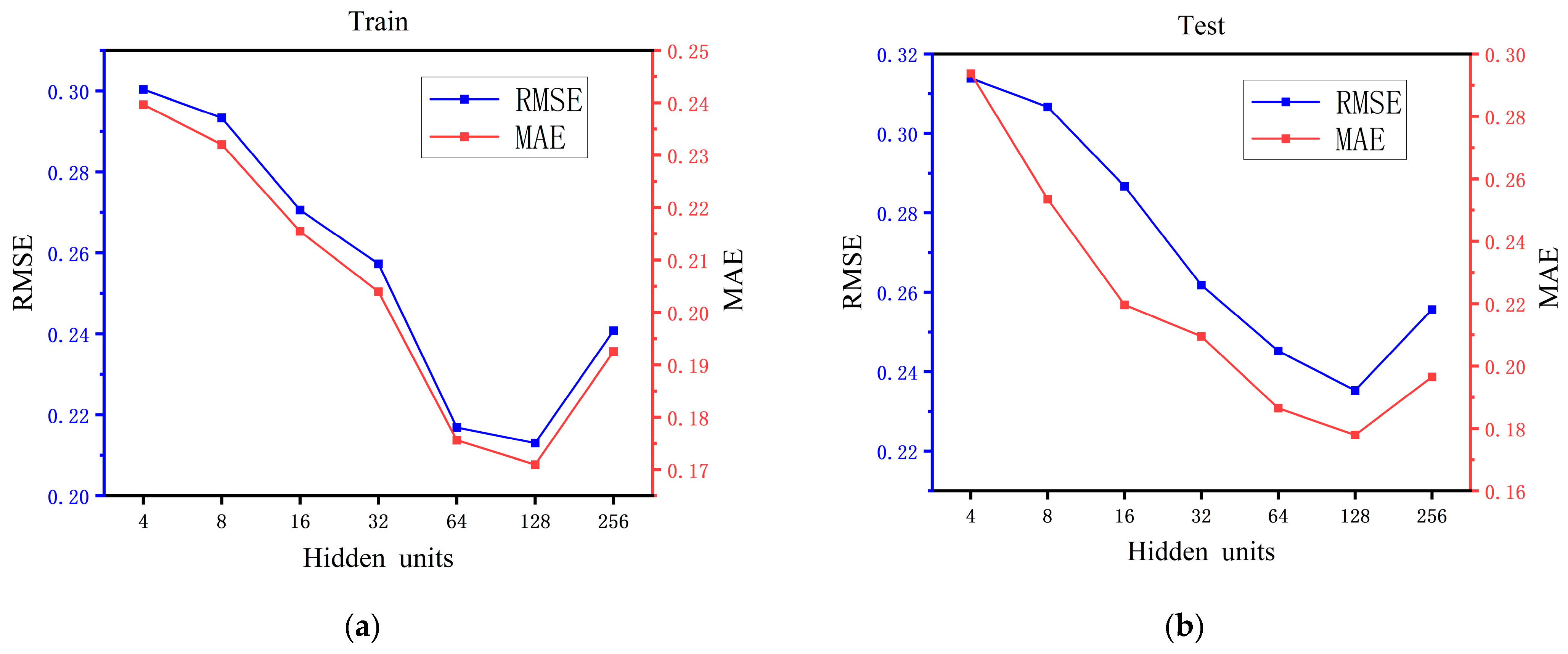
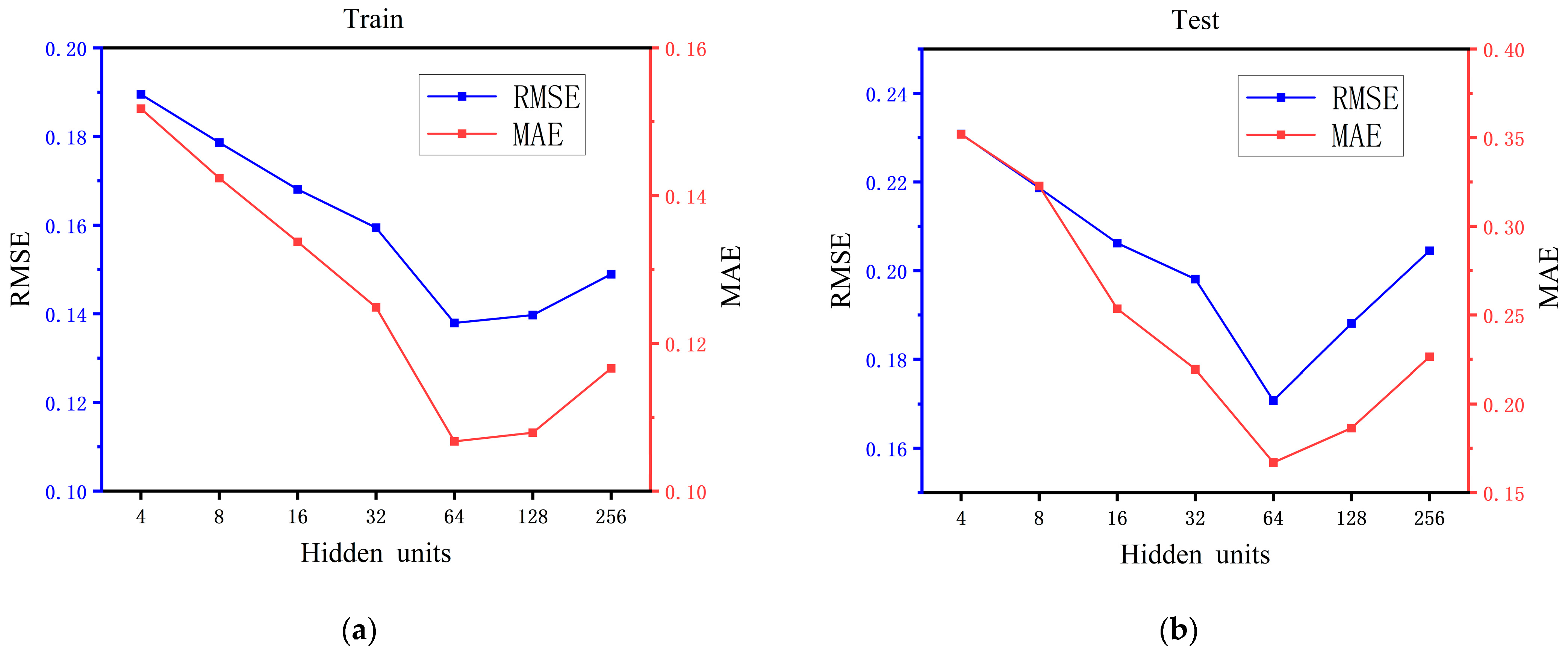
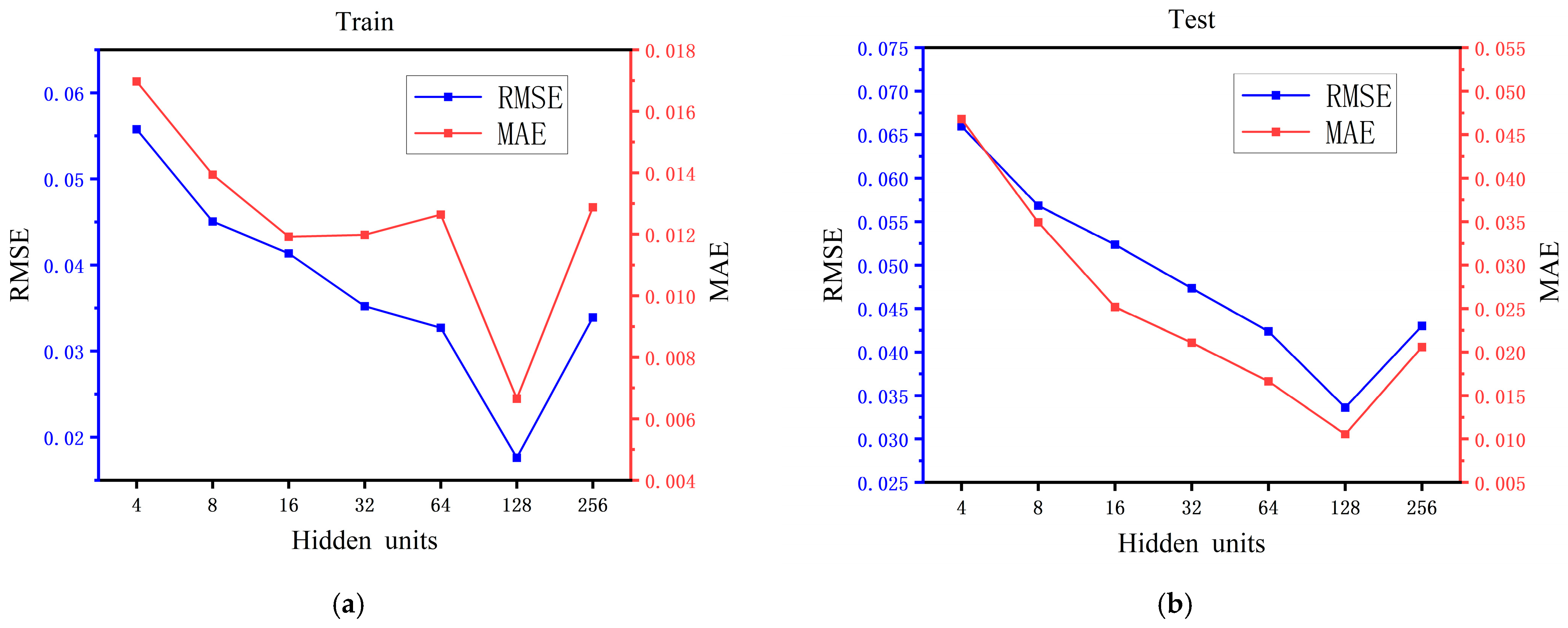
In the experiment, we selected and compared the prediction accuracy changes by choosing values from the set [4, 8, 16, 32, 64, 128, 256]. The experimental results are shown in Figure 7, Figure 8 and Figure 9, illustrating the significant impact of the number of hidden units on model performance. Figure 7 shows the prediction performance of the GCN model on the taxi trajectory dataset. When the number of hidden units reaches 128, both the RMSE and MAE for the training and test sets reach their best values. Figure 8 presents the prediction performance of the GCN model on the bike-sharing trajectory dataset. The results show that when the number of hidden units is 64, the model achieves the best prediction results on both the training and test sets. For the bus trajectory dataset, as shown in Figure 9, Figure 9a shows the RMSE and MAE results for the LSTM model on the training set. It can be observed that the model stabilizes when the number of LSTM units reaches 128. Figure 9b presents the prediction performance on the test set, where the best results are also achieved when the number of hidden units is 128. When the model stabilizes, the prediction accuracy is at its highest, and the prediction error is minimized. As the number of hidden units increases, the prediction accuracy shows a trend of first decreasing and then increasing. This is primarily because, when the number of hidden units exceeds a certain threshold, the model complexity and computational difficulty increase significantly, leading to overfitting [42].

5.3. Dynamic Weights Analysis of Multi-Model Ensemble

Based on the experiments above, the optimal hyperparameters of the models were determined, and the best prediction results were obtained. We further adopted a weighted average multi-model ensemble strategy to combine the predictions of the individual models. In this experiment, we assigned three weights: the weight for the bike-sharing prediction result ( ω 1 ), the weight for the bus prediction result ( ω 2 ), and the weight for the taxi prediction result ( ω 3 ).
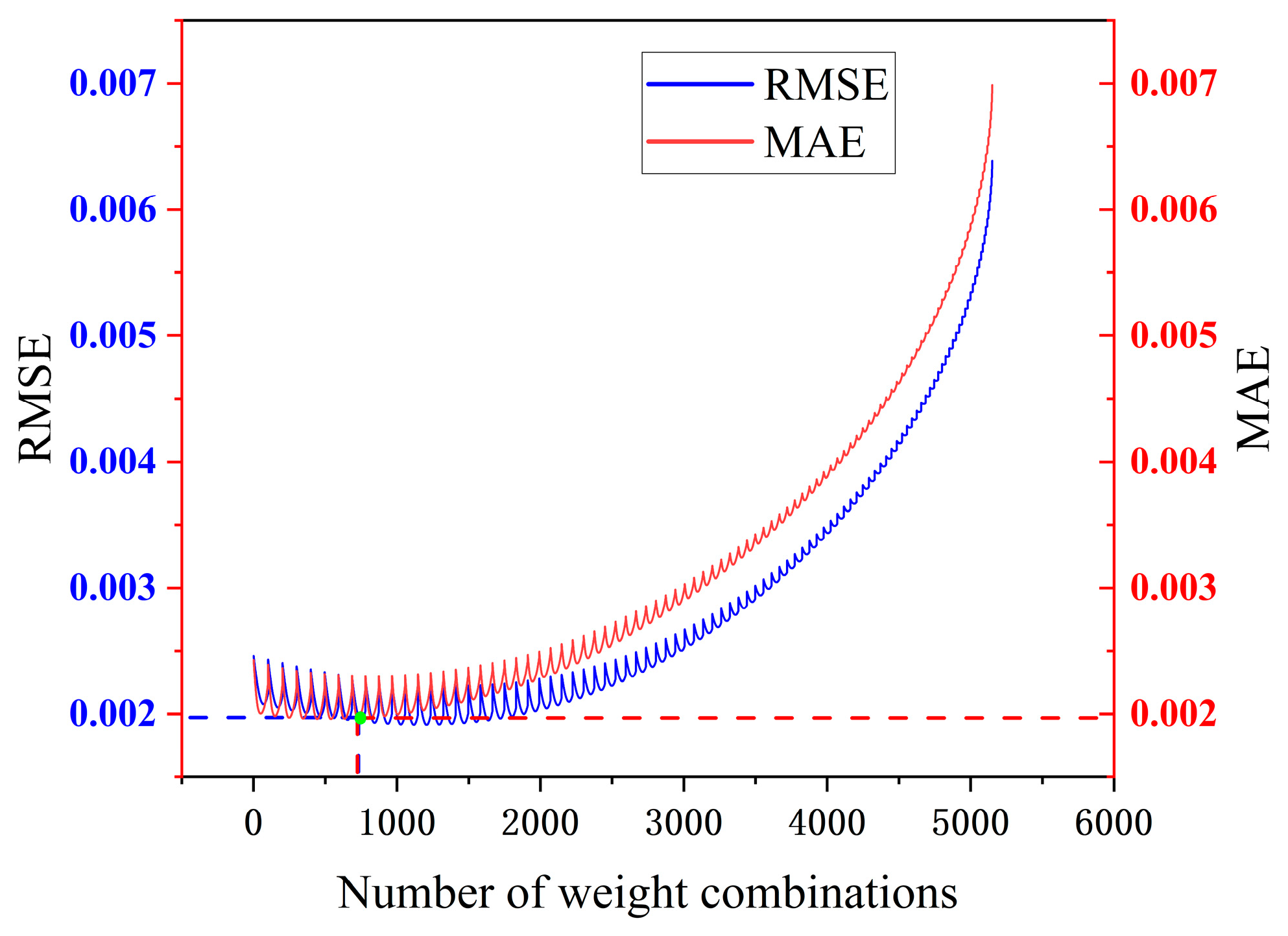
In all possible combinations of weights, we used RMSE and MAE as evaluation metrics to assess the prediction performance after weighted averaging. The weight combinations were calculated using Equation (14), and the possible combinations totaled 5151.
It was observed that when the weight combination number was 637 (indicated by the green point in Figure 10, with the weight distribution [ ω 1 , ω 2 , ω 3 ] = [0.25, 0.25, 0.50], the RMSE and MAE reached their minimum values of 0.0019624 and 0.0019597, respectively. This indicated that the model ensemble performance was optimal at this point. Afterward, the ensemble prediction results were subjected to denormalization and decoding, yielding trajectory positions in the same format as the original data.

5.4. Experimental Results

5.4.1. Comparison with Baselines

To better validate the prediction performance after the model ensemble phase, we conducted extensive experiments and compared the proposed method with the following eight methods, as shown in Table 2: (1) HMM [17], (2) LSTM [21], (3) Transformer [22], (4) DCRNN [6], (5) T-GCN [30], (6) STAEFormer [31], (7) 1DCNN-LSTM [34], and (8) DDGCRN [35]. The hyperparameters of these baseline methods were kept the same as those in the original articles or the published code.
The trajectory prediction results for the next time step are shown in Table 3. After the weighted fusion, our multi-model ensemble framework GLEN, in terms of prediction performance for both latitude (LAT) and longitude (LON) of the next trajectory point, significantly outperforms the other baseline models. This indicates that, in complex traffic networks, there are often strong interactive behaviors between the trajectory routes of different transportation modes. Therefore, the multi-model ensemble approach can more comprehensively capture the dynamic interactions between the trajectories of multimodal travel modes.
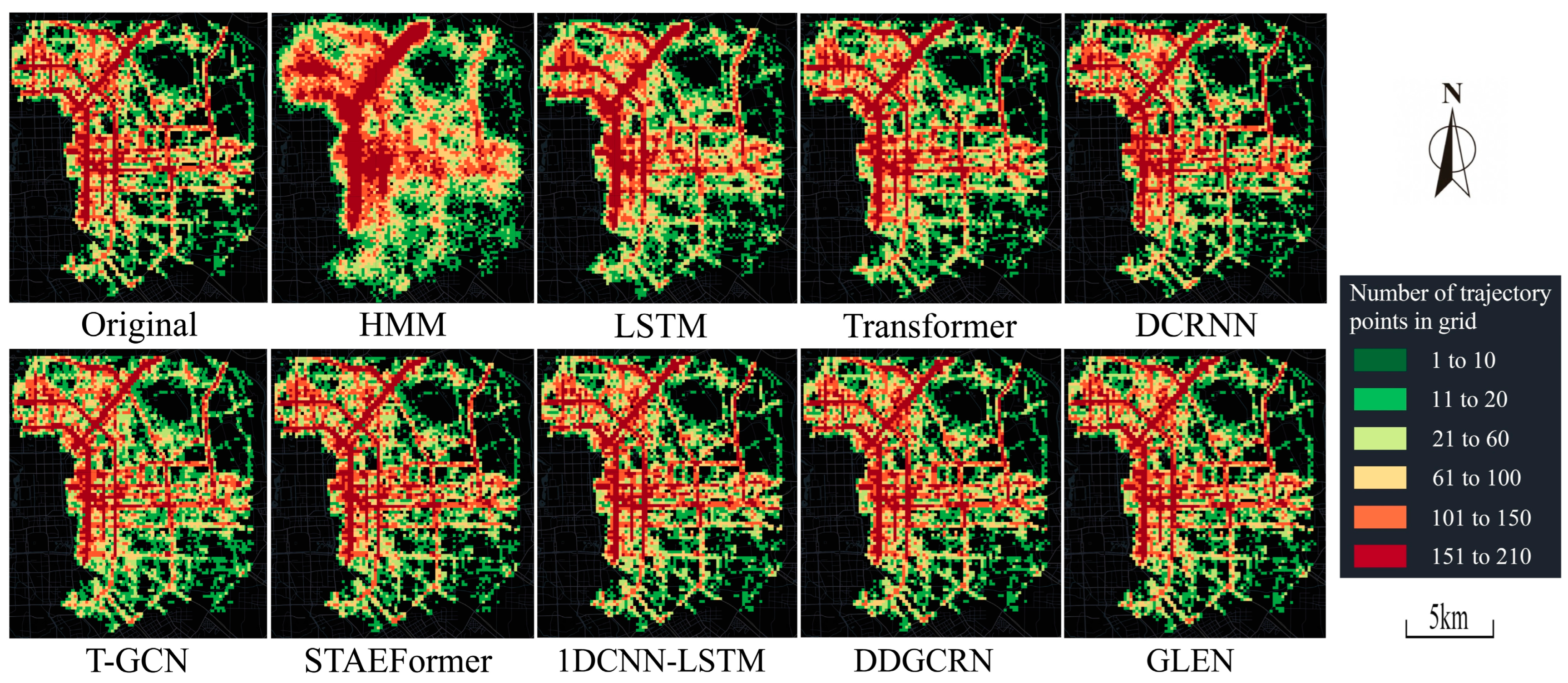
Compared to HMM, LSTM, Transformer, DCRNN, T-GCN, STAEFormer, 1DCNN-LSTM, and DDGCRN, the proposed method reduces the overall average MAE by 52.69%, 44.98%, 44.07%, 39.88%, 40.24%, 22.66%, 13.33%, and 5.01%, respectively. The overall average RMSE is reduced by 55.42%, 51.23%, 48.41%, 43.45%, 44.12%, 26%, 16.43%, and 8.03%, respectively. We predicted the results using different methods and calculated the total traffic using the flow fusion computation method, which was then visualized and analyzed, as shown in Figure 11. These results demonstrate that our multi-model ensemble framework GLEN outperforms all other models in both evaluation metrics, proving its effectiveness for spatiotemporal travel trajectory prediction tasks.
Further analysis reveals the following points: First, deep learning-based methods (including LSTM, Transformer, DCRNN, T-GCN, STAEFormer, 1DCNN-LSTM, DDGCRN, and GLEN) perform significantly better than the traditional HMM method, indicating that deep learning-based approaches are better at capturing nonlinear relationships. Second, spatiotemporal deep learning methods (including DCRNN, T-GCN, STAEFormer, 1DCNN-LSTM, DDGCRN, and GLEN) outperform Transformer and LSTM, highlighting the effectiveness of both temporal and spatial features in traffic trajectory prediction. Third, the GLEN, which models trajectory interactions between multimodal travel modes, performs better than STAEFormer, DCRNN, 1DCNN-LSTM, DDGCRN, and T-GCN. This indicates that constructing trajectory interaction between various transportation modes can more effectively simulate the interactions of traffic trajectories within the travel network.

5.4.2. Prediction Performance over Different Future Time Horizons

The experiment further tests the performance of the GLEN method in predicting the next two, three, and four time steps with every 15 min as a time step. The prediction results are shown in Table 4. When predicting the next two time steps, the overall average MAE and RMSE of this method were reduced by 2.52% and 1.96%, respectively, compared to the best baseline method. When predicting the next three time steps, the overall average MAE and RMSE were reduced by 1.46% and 1.42%, respectively. When predicting the next four time steps, the overall average MAE and RMSE were reduced by 1.67% and 0.52%, respectively.
It can be observed that when predicting fewer time points, the prediction errors of all models are smaller. As the trajectory prediction length increases, the prediction errors of each model gradually increase. This indicates that the prediction accuracy of the model decreases as the length of the trajectory points to be predicted increases. However, as the prediction sequence length increases, the proposed method consistently outperforms the baseline models at each prediction time point. Furthermore, even though the performance of all models decreases as the prediction length increases, the performance gap between GLEN and other baseline models generally widens. Therefore, it can be concluded that GLEN maintains good performance across different prediction time horizons.

5.4.3. Model Interpretation

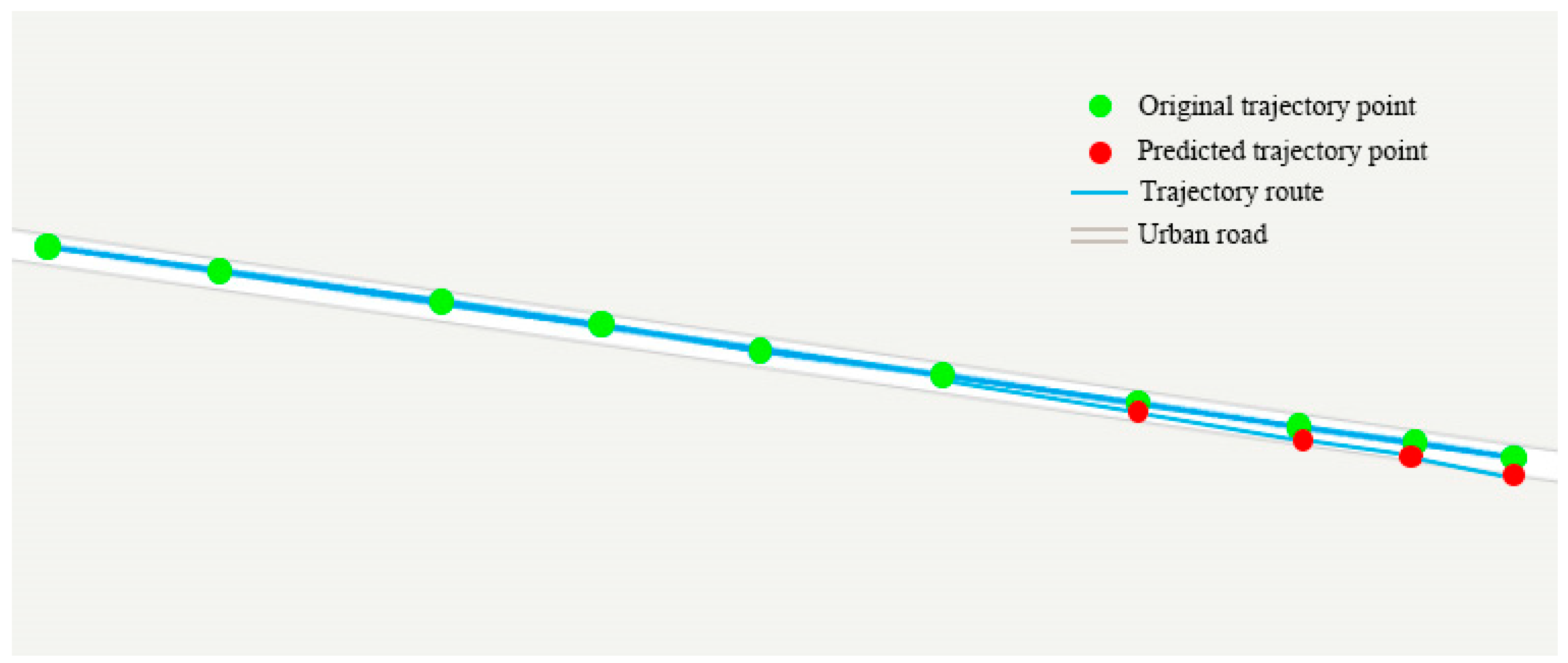
We performed a visual analysis on the test samples from the trajectory dataset to demonstrate the prediction performance of the proposed multi-model ensemble method. Figure 12 presents the prediction results for a real trajectory from the test data, focusing on the last four trajectory points of this segment. From the results, it is evident that the predicted values are very close to the actual trajectory points, reflecting the strong predictive capability of the method for travel trajectories. However, as the prediction length increases, the deviation from the actual travel trajectory becomes more noticeable. The green points represent the original trajectory points, while the red points represent the predicted trajectory points for the next one to four time steps.
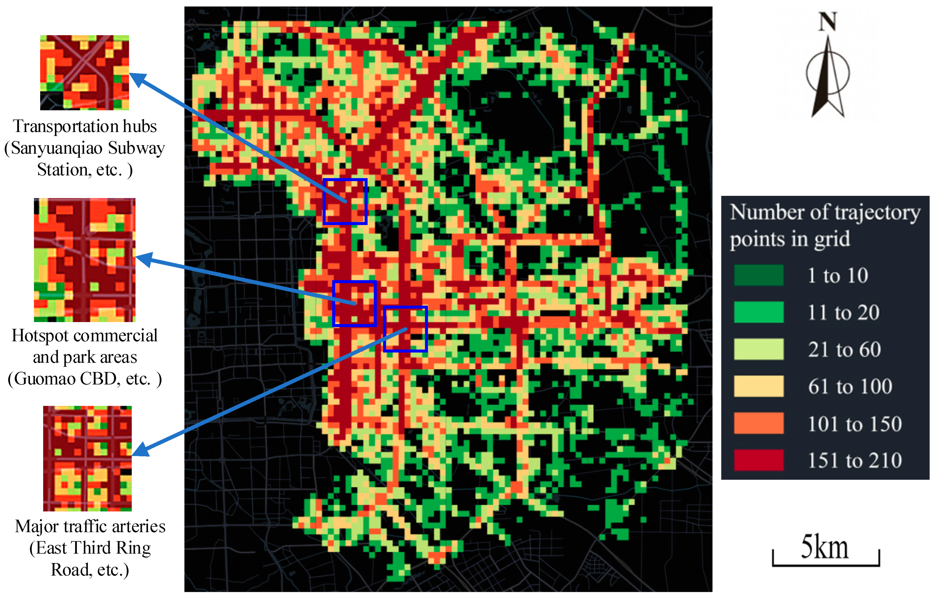
To provide a more comprehensive analysis and prediction of the changes in urban traffic trajectories, we visualized the trajectory points for the three types of transportation modes. As shown in Figure 13, the original trajectory points appear in several key areas, including hotspot commercial and park areas (e.g., Guomao CBD, Chaoyang Park, and Dongba Park), major traffic arteries (e.g., Jingtong Expressway, Chaoyang Road, and the East Third Ring Road), and transportation hubs (e.g., Sanyuanqiao Subway Station and Beijing Chaoyang Station). These areas usually become traffic hotspots due to the large flow of people, indicating that they may face greater traffic pressure. Figure 14a–d show the original trajectory route and the traffic trajectory trend of the next one to four time steps (each time step is 15 min). Through visual analysis, we can accurately identify the streets and areas where traffic congestion may occur in Chaoyang District in the future, and provide support for urban traffic management departments to take corresponding diversion measures in advance.

6. Discussion

This study aims to construct a flexible multimodal ensemble prediction framework through trajectory feature-driven adaptive model selection and dynamic weighted ensemble learning. The experimental results show that the GLEN framework outperforms the other methods presented in this paper in terms of both RMSE and MAE indicators. The matching of the model structure and travel mode specificity (GCN for dynamic travel scenarios and LSTM for fixed-route scenarios) is particularly effective. However, in the implementation process, we observe that under a finer time granularity, real-time adaptation to changing travel patterns still faces technical challenges, especially in the case of non-periodic congestion events or accidents.
Compared with classical models such as DCRNN [6], T-GCN [30], and 1DCNN-LSTM [34], these models usually focus on single travel mode or fixed network prediction, and the cross-modal integration of GLEN has made some progress. Unlike previous studies that usually rely on homogeneous feature assumptions, our method considers the diversity and dynamic interaction of urban traffic modes. Unlike DDGCRN [35], our method adjusts the graph structure locally according to the mode. Therefore, GLEN extends the previous research results by introducing a dynamic adjustment weight integration strategy.
However, the current research still has the following limitations. First, although our dataset is large, its geographical scope is limited to one district in Beijing, which may limit its generalization ability. Second, the current framework mainly defines cross-modal interaction as spatial proximity, which fails to fully incorporate the isolation effect of urban physical infrastructure (such as physical barriers like viaducts and bus lanes) and behavioral constraints (such as the avoidance behavior of drivers in mixed traffic environments). Third, in the scenario where only one travel mode (such as taxis or buses) is available, GLEN can be used as a single-flow predictor with the corresponding sub-model for prediction. The prediction quality is also affected by the accuracy and integrity of the trajectory data. Missing data or inaccurate timestamps in high-traffic grids may lead to traffic estimation bias.
GLEN’s multi-mode adaptability enables the traffic control center to dynamically predict congestion hotspots and recommend detour or mode conversion strategies. For example, during peak hours, GLEN can provide high-confidence predictions of bus overload or taxi travel availability. In addition, it also promotes optimal scheduling and resource allocation in urban traffic networks.

7. Conclusions

This study proposes GLEN, a spatiotemporal ensemble learning framework that integrates adaptive model selection and dynamic weight fusion for multimodal trajectory flow prediction. By aligning prediction models with mode-specific characteristics and capturing dependencies within and between patterns, GLEN outperforms existing methods across various metrics in a real case study of Beijing’s Chaoyang District.
Future research may explore the integration of real-time learning mechanisms, such as the online updating of model parameters and graph structures, to enhance adaptability in dynamic urban environments. Expanding the framework to larger spatial regions or applying it to different cities with heterogeneous transport infrastructures will help test the generalizability and robustness of the method. Additionally, incorporating user behavioral data or external events (e.g., weather or public events) may further improve prediction accuracy.
The findings have practical implications for intelligent transportation systems and urban mobility planning. GLEN’s multimodal coordination capability can support fine-grained traffic control, optimized public transit scheduling, and demand-responsive strategies.

Author Contributions

Zhenkai Wang performed the computations, completed the data collection and data preprocessing, and carried out the experiments. Lujin Hu conceived the presented idea, developed the theory, and verified the analytical methods. All authors discussed the results and contributed to the final manuscript. All authors have read and agreed to the published version of the manuscript.

Funding

This work was supported by the Beijing University of Civil Engineering and Architecture’s young teachers research ability enhancement program (x21023).

Data Availability Statement

The authors confirm that the Beijing bus data supporting the findings of this study are available from the website (https://blog.csdn.net/weixin_44172398) and the Beijing shared-bicycle data are available from the website (https://www.biendata.xyz), accessed on 12 August 2024. Additional data related to this study may be requested from the corresponding authors.

Conflicts of Interest

The authors declare no conflicts of interest.

References

  1. Ma, C.; Dai, G.; Zhou, J. Short-term traffic flow prediction for urban road sections based on time series analysis and LSTM_BILSTM method. IEEE Trans. Intell. Transp. Syst. 2021, 23, 5615–5624. [Google Scholar] [CrossRef]
  2. Zhou, T.; Huang, B.; Li, R.; Liu, X.; Huang, Z. An attention-based deep learning model for citywide traffic flow forecasting. Int. J. Digit. Earth 2022, 15, 323–344. [Google Scholar] [CrossRef]
  3. Wei, X.; Zhang, Y.; Wang, S.; Zhao, X.; Hu, Y.; Yin, B. Self-Attention Graph Convolution Imputation Network for Spatio-Temporal Traffic Data. IEEE Trans. Intell. Transp. Syst. 2024, 25, 19549–19562. [Google Scholar] [CrossRef]
  4. Gao, Y.; Fu, J.; Feng, W.; Xu, T.; Yang, K. Surrounding vehicle trajectory prediction under mixed traffic flow based on graph attention network. Physica A 2024, 639, 129643. [Google Scholar] [CrossRef]
  5. Cai, S.; Liu, G.; He, J.; Du, Y.; Si, Z.; Jiang, Y. Temporal-Spatial Traffic Flow Prediction Model Based on Prompt Learning. ISPRS Int. J. Geo-Inf. 2025, 14, 11. [Google Scholar] [CrossRef]
  6. Li, Y.; Yu, R.; Shahabi, C.; Liu, Y. Diffusion convolutional recurrent neural network: Data-driven traffic forecasting. arXiv 2017, arXiv:1707.01926. [Google Scholar]
  7. Zhang, J.; Zheng, Y.; Qi, D.; Li, R.; Yi, X.; Li, T. Predicting citywide crowd flows using deep spatio-temporal residual networks. Artif. Intell. 2018, 259, 147–166. [Google Scholar] [CrossRef]
  8. Dou, Z.; Guo, D. DPSTCN: Dynamic Pattern-Aware Spatio-Temporal Convolutional Networks for Traffic Flow Forecasting. ISPRS Int. J. Geo-Inf. 2025, 14, 10. [Google Scholar] [CrossRef]
  9. Benterki, A.; Judalet, V.; Maaoui, C.; Boukhnifer, M. Multi-model and learning-based framework for real-time trajectory prediction. In Proceedings of the 28th Mediterranean Conference on Control and Automation (MED), Saint-Raphaël, France, 15–18 September 2020; pp. 776–781. [Google Scholar] [CrossRef]
  10. Smith, B.L.; Demetsky, M.J. Traffic flow forecasting: Comparison of modeling approaches. J. Transp. Eng. 1997, 123, 261–266. [Google Scholar] [CrossRef]
  11. Hamed, M.M.; Al-Masaeid, H.R.; Said, Z.M.B. Short-term prediction of traffic volume in urban arterials. J. Transp. Eng. 1995, 121, 249–254. [Google Scholar] [CrossRef]
  12. Williams, B.M.; Durvasula, P.K.; Brown, D.E. Urban freeway traffic flow prediction: Application of seasonal autoregressive integrated moving average and exponential smoothing models. Transp. Res. Rec. 1998, 1644, 132–141. [Google Scholar] [CrossRef]
  13. Lee, S.; Fambro, D.B. Application of subset autoregressive integrated moving average model for short-term freeway traffic volume forecasting. Transp. Res. Rec. 1999, 1678, 179–188. [Google Scholar] [CrossRef]
  14. Davis, G.A.; Nihan, N.L. Nonparametric regression and short-term freeway traffic forecasting. J. Transp. Eng. 1991, 117, 178–188. [Google Scholar] [CrossRef]
  15. Lefèvre, S.; Laugier, C.; Ibañez-Guzmán, J. Exploiting map information for driver intention estimation at road intersections. In Proceedings of the 2011 IEEE Intelligent Vehicles Symposium (IV), Baden-Baden, Germany, 5–9 June 2011; pp. 583–588. [Google Scholar] [CrossRef]
  16. Hu, W.; Yan, L.; Liu, K.; Wang, H. A short-term traffic flow forecasting method based on the hybrid PSO-SVR. Neural Process. Lett. 2016, 43, 155–172. [Google Scholar] [CrossRef]
  17. Firl, J.; Stübing, H.; Huss, S.A.; Stiller, C. Predictive maneuver evaluation for enhancement of car-to-x mobility data. In Proceedings of the 2012 IEEE Intelligent Vehicles Symposium, Madrid, Spain, 3–7 June 2012; pp. 558–564. [Google Scholar] [CrossRef]
  18. Hussain, B.; Afzal, M.K.; Ahmad, S.; Mostafa, A.M. Intelligent traffic flow prediction using optimized GRU model. IEEE Access 2021, 9, 100736–100746. [Google Scholar] [CrossRef]
  19. Jia, Y.; Wu, J.; Du, Y. Traffic speed prediction using deep learning method. In Proceedings of the 2016 IEEE 19th International Conference on Intelligent Transportation Systems (ITSC), Rio de Janeiro, Brazil, 1–4 November 2016; pp. 1217–1222. [Google Scholar] [CrossRef]
  20. Lv, Y.; Duan, Y.; Kang, W.; Li, Z.; Wang, F.-Y. Traffic flow prediction with big data: A deep learning approach. IEEE Trans. Intell. Transp. Syst. 2014, 16, 865–873. [Google Scholar] [CrossRef]
  21. Sattarzadeh, A.R.; Kutadinata, R.J.; Pathirana, P.N.; Huynh, V.T. A novel hybrid deep learning model with ARIMA Conv-LSTM networks and shuffle attention layer for short-term traffic flow prediction. Transp. A Transp. Sci. 2023, 21, 2236724. [Google Scholar] [CrossRef]
  22. Liu, Y.; Zhang, J.; Fang, L.; Jiang, Q.; Zhou, B. Multimodal motion prediction with stacked transformers. arXiv 2021. [Google Scholar] [CrossRef]
  23. Ma, X.; Tao, Z.; Wang, Y.; Yu, H.; Wang, Y. Long short-term memory neural network for traffic speed prediction using remote microwave sensor data. Transp. Res. Part C Emerg. Technol. 2015, 54, 187–197. [Google Scholar] [CrossRef]
  24. Zhang, D.; Kabuka, M.R. Combining weather condition data to predict traffic flow: A GRU-based deep learning approach. IET Intel. Transp. Syst. 2018, 12, 578–585. [Google Scholar] [CrossRef]
  25. Liu, Y.; Zheng, H.; Feng, X.; Chen, Z. Short-term traffic flow prediction with Conv-LSTM. In Proceedings of the 9th International Conference on Wireless Communications and Signal Processing (WCSP), Nanjing, China, 11–13 October 2017; pp. 1–6. [Google Scholar] [CrossRef]
  26. Yu, H.; Wu, Z.; Wang, S.; Wang, Y.; Ma, X. Spatiotemporal recurrent convolutional networks for traffic prediction in transportation networks. Sensors 2017, 17, 1501. [Google Scholar] [CrossRef]
  27. Wang, J.; Gu, Q.; Wu, J.; Liu, G.; Xiong, Z. Traffic speed prediction and congestion source exploration: A deep learning method. In Proceedings of the IEEE 16th International Conference on Data Mining (ICDM), Barcelona, Spain, 12–15 December 2016; pp. 499–508. [Google Scholar] [CrossRef]
  28. Gong, S.; Liu, J.; Yang, Y.; Cai, J.; Xu, G.; Cao, R.; Jing, C.; Liu, Y. Self-paced Gaussian-based graph convolutional network: Predicting travel flow and unravelling spatial interactions through GPS trajectory data. Int. J. Digit. Earth 2024, 17, 2353123. [Google Scholar] [CrossRef]
  29. Qi, T.; Li, G.; Chen, L.; Xue, Y. ADGCN: An asynchronous dilation graph convolutional network for traffic flow prediction. IEEE Internet Things J. 2021, 9, 4001–4014. [Google Scholar] [CrossRef]
  30. Zhao, L.; Song, Y.; Zhang, C.; Liu, Y.; Wang, P.; Lin, T.; Deng, M.; Li, H. T-GCN: A temporal graph convolutional network for traffic prediction. IEEE Trans. Intell. Transp. Syst. 2019, 21, 3848–3858. [Google Scholar] [CrossRef]
  31. Liu, H.; Dong, Z.; Jiang, R.; Deng, J.; Deng, J.; Chen, Q.; Song, X. STAEformer: Spatio-Temporal Adaptive Embedding Makes Vanilla Transformer SOTA for Traffic Forecasting. arXiv 2023. [Google Scholar] [CrossRef]
  32. Patara, T.; Lee, J.G. DF-TAR: A Deep Fusion Network for Citywide Traffic Accident Risk Prediction with Dangerous Driving Behavior. In Proceedings of the Web Conference 2021 (WWW’21), New York, NY, USA, 19–23 April 2021; pp. 1146–1156. [Google Scholar] [CrossRef]
  33. Choi, J.; Choi, H.; Hwang, J.; Park, N. Graph neural controlled differential equations for traffic forecasting. In Proceedings of the AAAI Conference on Artificial Intelligence, Palo Alto, CA, USA, 22 February–1 March 2022; pp. 6367–6374. [Google Scholar] [CrossRef]
  34. Wang, K.; Ma, C.; Qiao, Y.; Lu, X.; Hao, W.; Dong, S. A hybrid deep learning model with 1DCNN-LSTM-Attention networks for short-term traffic flow prediction. Physica A 2021, 583, 126293. [Google Scholar] [CrossRef]
  35. Weng, W.; Fan, J.; Wu, H.; Hu, Y.; Tian, H.; Zhu, F.; Wu, J. A Decomposition Dynamic graph convolutional recurrent network for traffic forecasting. Pattern Recognit. 2023, 142, 109670. [Google Scholar] [CrossRef]
  36. Fernando, T.; Denman, S.; Sridharan, S.; Fookes, C. Soft+ hardwired attention: A lstm framework for human trajectory prediction and abnormal event detection. Neural Netw. 2018, 108, 466–478. [Google Scholar] [CrossRef]
  37. Li, Y.; Tarlow, D.; Brockschmidt, M.; Zemel, R. Gated graph sequence neural networks. arXiv 2015, arXiv:1511.05493. [Google Scholar]
  38. Ke, J.; Qin, X.; Yang, H.; Zheng, Z.; Zhu, Z.; Ye, J. Predicting origin-destination ride-sourcing demand with a spatio-temporal encoder-decoder residual multi-graph convolutional network. Transp. Res. Part C Emerg. Technol. 2021, 122, 102858. [Google Scholar] [CrossRef]
  39. Qin, H.; Yang, X. Iterative Algorithm for Vessel Trajectory Restoration Based on Improved Linear Interpolation. J. Comput.-Aided Des. Comput. Graph. 2019, 31, 1759–1767. [Google Scholar] [CrossRef]
  40. Wei, X. Analytic Deep Learning: Convolutional Neural Network Principles and Visual Practice, 1st ed.; Publishing House of Electronics Industry: Beijing, China, 2018; pp. 21–109. [Google Scholar]
  41. Kim, G.; Kim, D.; Ahn, Y.; Huh, K. Hybrid approach for vehicle trajectory prediction using weighted integration of multiple models. IEEE Access 2021, 9, 78715–78723. [Google Scholar] [CrossRef]
  42. Lv, M.; Hong, Z.; Chen, L.; Chen, T.; Zhu, T.; Ji, S. Temporal multi-graph convolutional network for traffic flow prediction. IEEE Trans. Intell. Transp. Syst. 2020, 22, 3337–3348. [Google Scholar] [CrossRef]
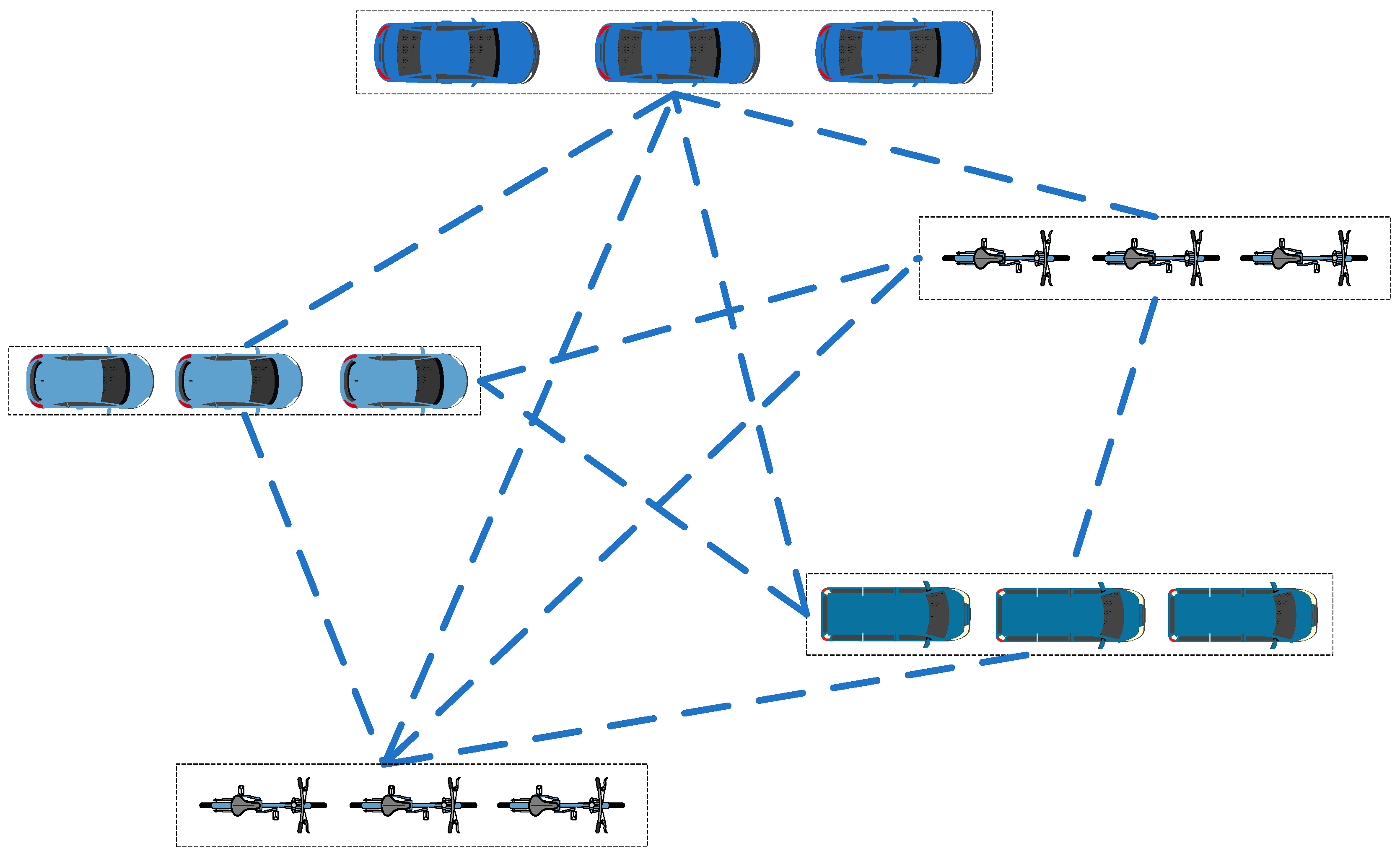
Figure 1. Trajectory interaction in graph structure description.
Ijgi 14 00308 g001
Figure 2. Study area.
Ijgi 14 00308 g002
Figure 3. Overall research framework.
Ijgi 14 00308 g003
Figure 4. Dynamic travel prediction framework.
Ijgi 14 00308 g004
Figure 5. Fixed-route prediction framework.
Ijgi 14 00308 g005
Figure 6. Loss curves of different models during training and validation.
Ijgi 14 00308 g006
Figure 7. Comparison of prediction performance between the training and test sets with different hidden units based on the taxi trajectory dataset. (a) Variation in RMSE and MAE in the training set. (b) Variation in RMSE and MAE in the test set.
Ijgi 14 00308 g007
Figure 8. Comparison of prediction performance between the training and test sets with different hidden units based on the bike-sharing trajectory dataset. (a) Variation in RMSE and MAE in the training set. (b) Variation in RMSE and MAE in the test set.
Ijgi 14 00308 g008
Figure 9. Comparison of prediction performance between the training and test sets with different hidden units based on the bus trajectory dataset. (a) Variation in RMSE and MAE in the training set. (b) Variation in RMSE and MAE in the test set.
Ijgi 14 00308 g009
Figure 10. Ensemble performance with different weight combinations.
Ijgi 14 00308 g010
Figure 11. Comparison of the total traffic flow distribution predicted by the different methods.
Ijgi 14 00308 g011
Figure 12. Prediction results of specific trajectory at multiple future time steps.
Ijgi 14 00308 g012
Figure 13. Distribution of original trajectory points.
Ijgi 14 00308 g013
Figure 14. (ad) show the trajectory distributions for the next one to four time steps, respectively.
Ijgi 14 00308 g014
Table 1. Partial data example of vehicle trajectory.
DateOrder IDLongitudeLatitudePassenger
Status
Direction Angle
2019/5/27 16:00:09861729202470116.486439.99074039
2019/5/27 16:12:32861729202470116.4974740.00511000
2019/5/27 16:30:15861729202470116.5243440.01903063
2019/5/27 16:46:44861729202470116.4386639.985390297
2019/9/27 17:10:15861729202470116.4012639.98960168
Table 2. Baseline methodology and characteristics.
Baseline MethodsCharacteristics of Model Methods
HMMThe Hidden Markov Model generates unobservable state sequences through a hidden Markov chain and uses these state sequences to generate observed value sequences.
LSTMTraffic trajectory prediction is performed using the LSTM model. In the experiment, two LSTM layers are stacked, with each layer containing 32 units.
TransformerThe model uses partial trajectory data. By extracting and analyzing the spatial and temporal characteristics of the trajectory, the future trajectory points of the traveler can be accurately predicted.
DCRNNTraffic trajectories are modeled as diffusion processes on graphs, and a deep learning framework is proposed that combines both spatial and temporal correlations.
T-GCNCombines GCN and GRU for traffic trajectory prediction. It performs graph convolution operations while considering only the topology of the graph.
STAEFormerThe autoencoder and Transformer architecture are integrated, and the local and global feature patterns are captured by the self-attention mechanism. The spatiotemporal data is effectively compressed by the autoencoder, and the spatiotemporal relationship is modeled in parallel.
1DCNN-LSTMDeveloped an integrated prediction model based on an attentional mechanism and a 1DCNN-LSTM network, which combines the advantages of both models.
DDGCRNThis is a dual dynamic graph convolutional recurrent network, which combines RNNs to model complex spatiotemporal dependencies and dynamically adjusts the graph structure.
Table 3. Prediction accuracy of different models for a trajectory in the future.
Future
Moments
ModelsLatitudeLongitude
MAERMSEMAERMSE
HMM0.63520.67850.64450.7133
LSTM0.54720.61730.55320.6547
Transformer0.53830.59620.54420.6063
DCRNN0.49810.55360.50890.5434
1T-GCN0.51780.56320.49530.5471
STAEFormer0.38570.42260.39710.4158
1DCNN-LSTM0.36640.39750.33210.3449
DDGCRN0.32890.34580.30840.3244
GLEN0.32270.32420.28270.2962
Table 4. Prediction accuracy of different models for multiple trajectories in the future.
Future
Moments
ModelsLatitudeLongitude
MAERMSEMAERMSE
HMM0.68450.70310.67680.7482
LSTM 0.61780.66830.62280.6945
Transformer0.59720.62140.58630.6487
DCRNN0.55720.58430.54230.5901
2T-GCN 0.58740.59320.56740.5943
STAEFormer0.50970.53760.50180.5139
1DCNN-LSTM0.45340.49570.45420.4587
DDGCRN0.42880.44130.42710.4125
GLEN0.40410.44580.43020.3913
HMM0.71520.73450.71620.7643
LSTM 0.64580.67340.62540.6653
Transformer0.59860.65980.60520.6263
DCRNN0.52440.54370.54770.5245
3T-GCN 0.54820.56680.55350.5611
STAEFormer0.49540.52120.53190.5483
1DCNN-LSTM0.47570.49110.49210.5171
DDGCRN0.45810.43120.42840.4692
GLEN0.45240.43320.42120.4544
HMM0.81010.82510.77400.7962
LSTM0.72310.74080.70060.7235
Transformer0.65870.68020.65770.6947
DCRNN0.59100.61280.60070.6255
4T-GCN 0.60120.60450.63010.6387
STAEFormer0.55670.57360.58100.5875
1DCNN-LSTM0.53810.54060.52210.5351
DDGCRN0.48320.48960.49320.4824
GLEN0.49040.48680.46970.4801
Disclaimer/Publisher’s Note: The statements, opinions and data contained in all publications are solely those of the individual author(s) and contributor(s) and not of MDPI and/or the editor(s). MDPI and/or the editor(s) disclaim responsibility for any injury to people or property resulting from any ideas, methods, instructions or products referred to in the content.