Predicting the Next Location of Urban Individuals via a Representation-Enhanced Multi-View Learning Network

Abstract

Accurately predicting the next location of urban individuals is a central issue in human mobility research. Human mobility exhibits diverse patterns, requiring the integration of spatiotemporal contexts for location prediction. In this context, multi-view learning has become a prominent method in location prediction. Despite notable advances, current methods still face challenges in effectively capturing non-spatial proximity of regional preferences, complex temporal periodicity, and the ambiguity of location semantics. To address these challenges, we propose a representation-enhanced multi-view learning network (ReMVL-Net) for location prediction. Specifically, we propose a community-enhanced spatial representation that transcends geographic proximity to capture latent mobility patterns. In addition, we introduce a multi-granular enhanced temporal representation to model the multi-level periodicity of human mobility and design a rule-based semantic recognition method to enrich location semantics. We evaluate the proposed model using mobile phone data from Fuzhou. Experimental results show a 2.94% improvement in prediction accuracy over the best-performing baseline. Further analysis reveals that community space plays a key role in narrowing the candidate location set. Moreover, we observe that prediction difficulty is strongly influenced by individual travel behaviors, with more regular activity patterns being easier to predict.

1. Introduction

In urban environments, human mobility serves as a link connecting urban structures [1]. Understanding human mobility patterns can support urban planning and management, thereby contributing to sustainable urban development [2]. Today, approximately 85% of the global population owns smartphones [3]. The widespread availability of mobile location data offers an unprecedented foundation for understanding human mobility patterns. Numerous studies have shown that human mobility exhibits spatiotemporal regularities and is highly predictable [4,5]. Accurate prediction of human mobility holds considerable value for downstream applications, including epidemic control [6], business recommendations [7], and traffic optimization [8,9,10,11].

Next location prediction refers to predicting the location urban individuals are likely to visit in the future based on their historical trajectories. For mobile users, predicting the next location aids in proactive route planning and points of interest (POIs) recommendation, thereby improving personalized travel services. Unlike traditional recommendation systems, location prediction inherently involves spatiotemporal dependencies [4,5]. A key challenge in location prediction lies in integrating heterogeneous features to generate effective recommendations, requiring a robust framework to combine these diverse features [12]. Various factors, including spatial patterns, temporal periodicity, and travel semantics, influence human mobility. Early studies primarily focused on the sequential patterns of trajectories, often neglecting the relevant context of human mobility [12,13]. The omission of critical information led to unsatisfactory prediction performance. With advancements in deep learning techniques, researchers have begun exploring methods for integrating spatiotemporal context [14]. Multi-view learning provides an effective solution by integrating heterogeneous features to enhance models’ expressive power [15].

Previous studies have examined key travel features, such as spatial patterns, temporal periodicity, and travel semantics. However, due to the heterogeneous and complex nature of spatiotemporal contexts, existing studies still face challenges in effectively capturing non-spatial proximity of regional preferences, complex temporal periodicity, and the ambiguity of location semantics. Specifically regarding spatial patterns, human mobility is typically confined to a specific spatial range, characterized by frequent movement between a limited number of locations. Regional preference has been introduced to describe this type of spatial pattern [16,17]. Existing studies primarily delineate regions based on geographic coordinates to capture human regional preferences [18,19]. However, human mobility does not always conform to the assumption of spatial proximity, such as cross-regional jumps during metro commutes. Relying solely on geographic distance in spatial modeling may fail to accurately capture human mobility patterns. Limited research has explored the use of implicit community structures formed by human mobility. Community space not only reflects the typical geographical extent of individual activities but also reveals the influence of group interactions on individual mobility behavior. From a temporal perspective, previous research has demonstrated that human mobility exhibits significant multi-granular periodic patterns, such as daily and weekly travel habits [5]. Effectively modeling the multi-granular periodicity of human mobility is expected to improve the accuracy of location prediction, yet existing methods lack robust mechanisms to model these hierarchical temporal dependencies. Regarding travel semantics, humans’ travel intentions significantly influence their choice of destinations [20]. However, global navigation satellite system (GNSS) datasets provide only location information and cannot directly infer travel purposes. Moreover, the complexity of urban environments introduces ambiguous location semantics. A single location may serve different purposes for different individuals. Existing studies often rely on external POI data for semantic inference [21]. However, these approaches encounter challenges in resolving ambiguity, which may affect the prediction results due to mismatches.

To address these challenges, we propose a representation-enhanced multi-view learning network (ReMVL-Net) for location prediction. This network integrates representation-enhanced spatial, temporal, and semantic view-specific encoders to achieve comprehensive mobility pattern modeling, thereby enabling a more precise understanding of human mobility patterns. The specific contributions of this study are as follows:

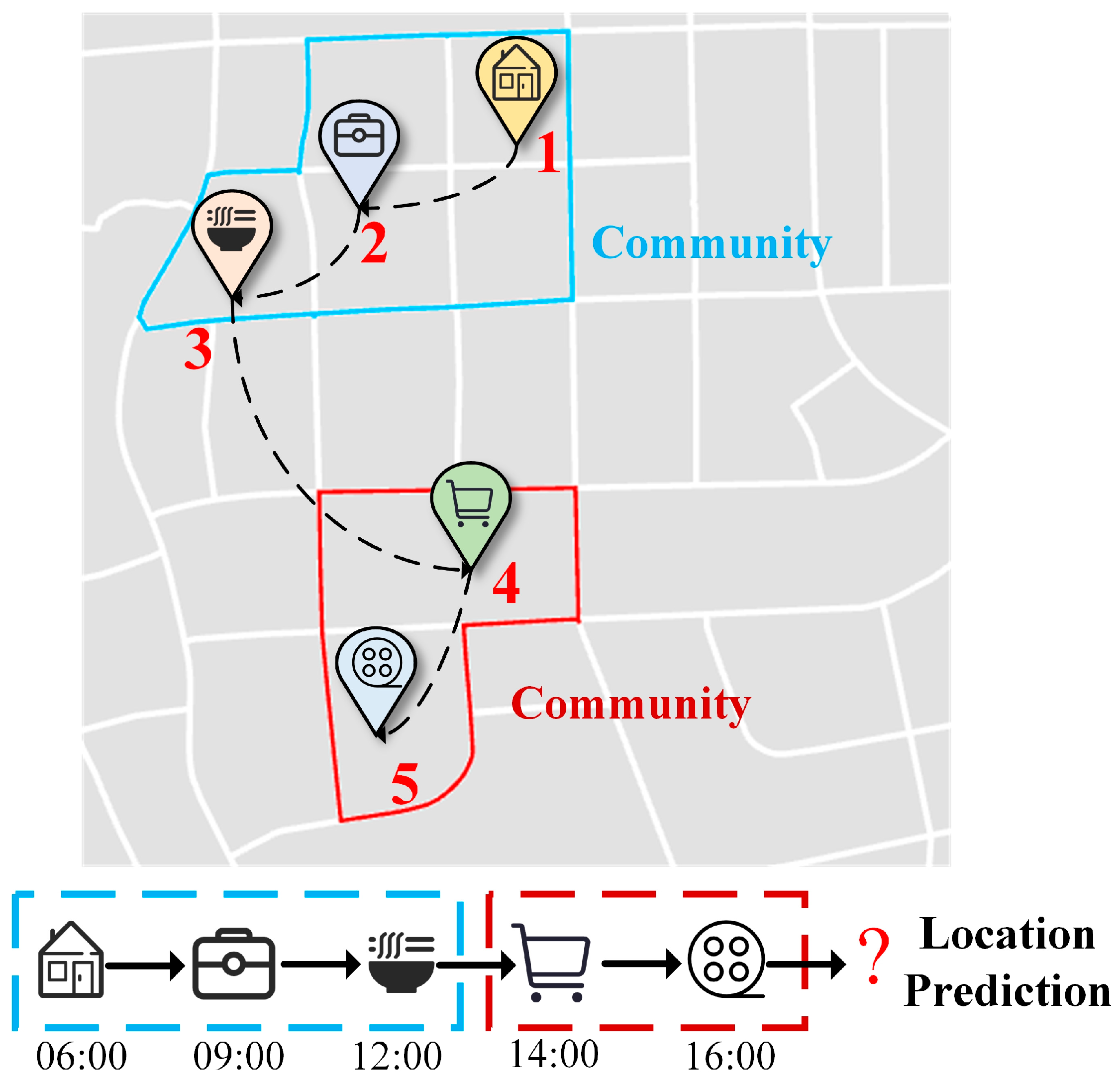
• We propose a novel community-enhanced spatial representation to capture human regional preferences and the relationships between locations. Accurately modeling human mobility patterns at different spatial scales improves the model’s understanding of spatial structure;
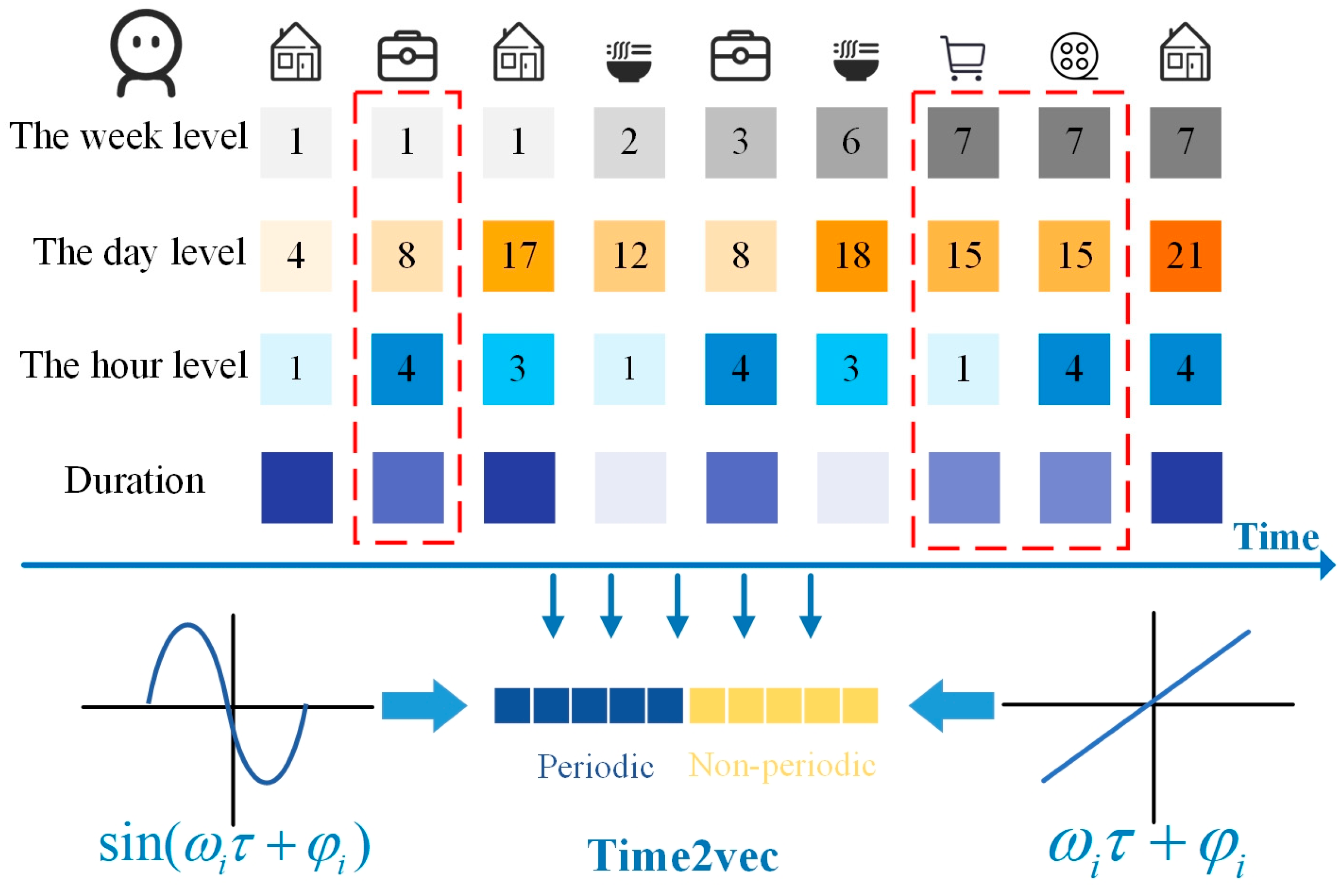
• We introduce a multi-granular enhanced temporal representation to capture complex temporal periodicity. Accurately modeling human mobility at different temporal granularities improves the model’s ability to learn temporal patterns;
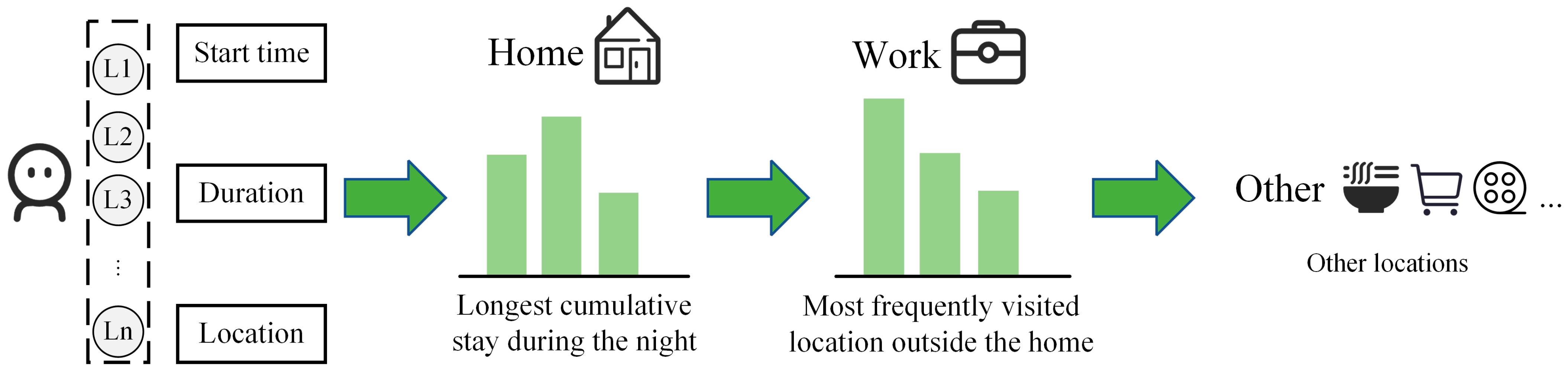
• We design a travel semantic recognition mechanism based on rule inference. This mechanism effectively distinguishes the functional meaning of the same location for different individuals, improving the model’s ability to perceive individualized travel intentions;
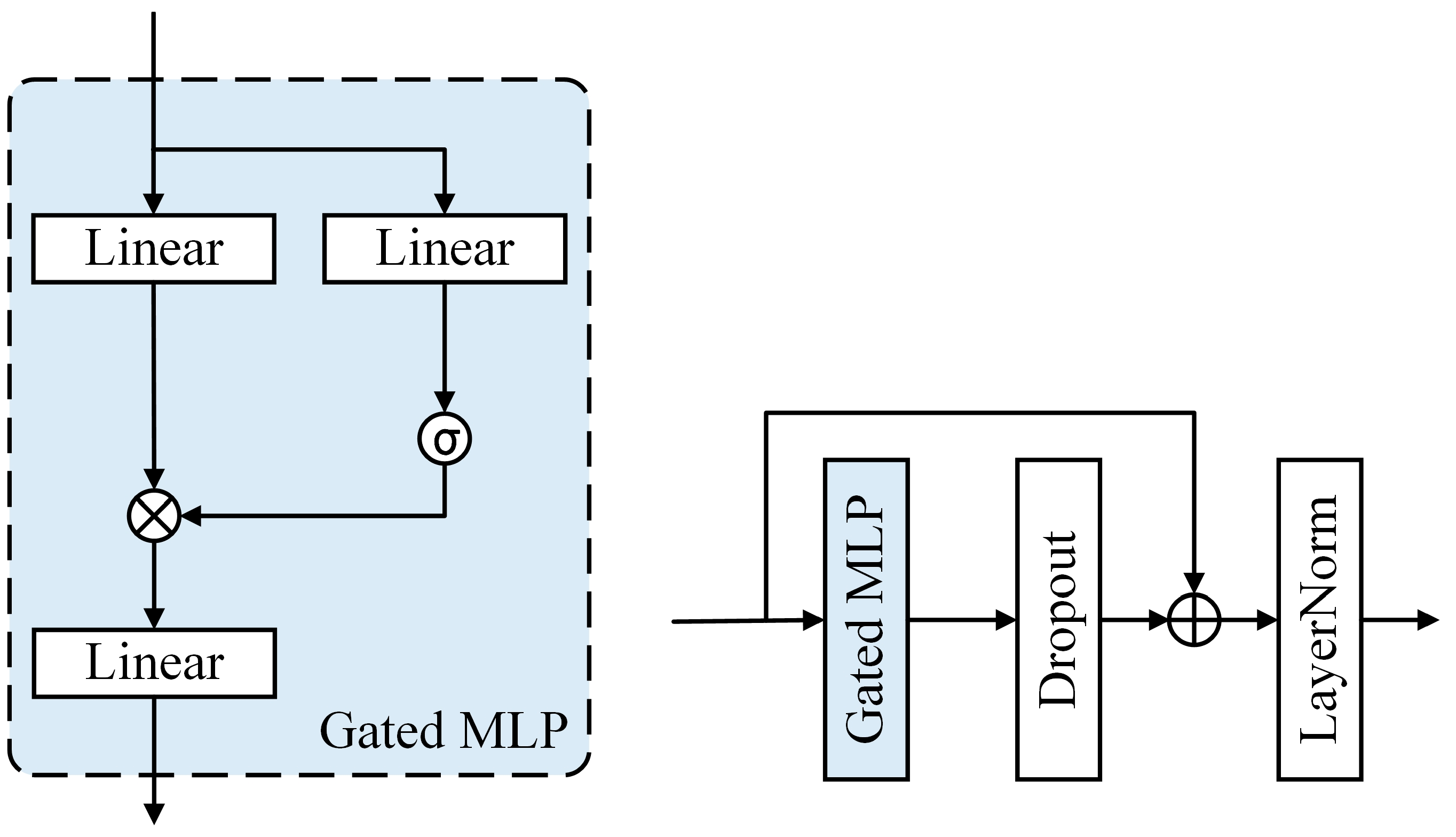
• We develop a transformer-based framework to capture global context dependencies and design a gated residual network to efficiently integrate spatial–temporal contexts and user features, thereby enhancing the model’s ability to capture the diversity of human mobility patterns.

2. Related Work

2.1. Next Location Prediction Methods

Next location prediction aims to predict the likely future destinations based on historical trajectories. Early location prediction studies primarily focused on sequential pattern mining from trajectories, with the Markov chain model being the most widely used method for location prediction [13,22]. Ashbrook and Starner [23] were the first to use GNSS datasets for location prediction, developing a user-specific Markov model. However, Markov models fail to capture complex higher-order sequence patterns, limiting their predictive accuracy.

Recurrent neural networks (RNNs) overcome the limitations of Markov chains by capturing sequential information through cyclic mechanisms and internal memory units [24,25]. Endo et al. [26] employed an RNN-based model to predict destinations, incorporating spatial proximity to control transition probabilities. The DeepMove model is based on RNNs to capture sequential transition patterns and incorporates a historical attention module to leverage the periodicity of human mobility [27]. However, RNNs suffer from long-range dependencies, often forgetting earlier information when modeling long sequences, which impairs their ability to capture long-term preferences.

Attention-based neural networks simulate the human mechanism of attending to critical information, enabling more effective capture of long-range dependencies [28,29]. Seongjin et al. [30] applied the attention mechanism to integrate network traffic state data for urban vehicle trajectory prediction. Tsiligkaridis et al. [31] employed transformer networks to predict destinations based on partial trajectories. However, this approach relies solely on location sequences and neglects richer contextual information.

2.2. Multi-View Learning for Next-Location Prediction

Multi-view learning improves model expressiveness by integrating heterogeneous features. Recent studies have explored the integration of multi-view information into deep learning models to enhance location prediction accuracy. For instance, Yao et al. [32] jointly modeled individual, location, time, and semantic information to construct a semantics-enriched recurrent model (SERM) based on long short-term memory (LSTM). Hong et al. [21] utilize a multi-head self-attentional (MHSA) model to capture location transition patterns based on historical visits, multi-scale temporal features, visit durations, and surrounding land use functions. Yang et al. [33] proposed GETNext, a graph-enhanced transformer that incorporates global trajectory flows, user preferences, spatiotemporal contexts, and time-aware category embeddings to effectively capture collaborative signals and enhance next POI prediction performance. Zheng and Zhou [34] proposed a multifactor user preference based on transformer (MUPT) model, which consists of a global POI relationship modeling, a local multi-factor user preference modeling and a prediction module. Spatial, temporal, semantic, and other contextual information have proven to be effective for location prediction.

Regarding spatial patterns, human mobility is typically concentrated in specific regions, and several studies have leveraged regional preferences to enhance location prediction. Song et al. [16] applied a density-based spatial clustering of applications with noise (DBSCAN) algorithm to cluster visited locations and derive regional preferences based on check-in frequencies. Sun et al. [17] applied the K-means algorithm to cluster POIs based on latitude and longitude, capturing their coarse-grained spatial distribution. Haifeng et al. [18] employed DBSCAN to partition the map into high-density and low-density regions based on location density, introducing an enhanced DeepMove model incorporating regional information. However, geographical clustering methods fail to account for non-spatial proximity of human mobility and struggle to delineate the boundaries of preferred activity regions. With the advancement of complex network techniques, researchers have extensively explored human mobility interactions in urban spaces [35]. Community detection has emerged as a key approach for studying urban spatial dynamics [36]. Community detection partitions networks into node groups with dense intra-group and sparse inter-group connections, thereby revealing community structures. Compared with regions formed through geographic clustering, community-based spatial units exhibit stronger interaction dynamics. However, the effective application of community spaces in location prediction requires further exploration.

Human mobility exhibits significant temporal periodicity [37]. Gao et al. [38] divided a day into 24 segments and performed location prediction by aggregating check-in preferences across different time periods. Luo et al. [39] introduced a spatiotemporal attention network (STAN) that leverages relative spatiotemporal information from check-in sequences. Wen et al. [40] employed Time2vec to model temporal periodicity at an hourly interval. However, while these studies account for temporal influence, they fail to fully capture the multi-granular periodicity of human mobility. For instance, commuting patterns are influenced not only by peak hours but also by weekday trends. Additionally, activity duration plays a crucial role, as the length of stay is closely linked to travel intent [41].

In terms of travel semantics, GNSS datasets lack semantic information, making it challenging to extract travel semantics. Some researchers have proposed utilizing external POI data to infer regional land function semantics as a proxy for travel semantics. Yao et al. [42] applied the TF-IDF method to generate regional land function semantic vectors for mobile individual location prediction. Hong et al. [21] employed POI data and an LDA model to capture land use context across multiple spatial scales. However, urban spaces are complex, and the same geographic unit can serve multiple purposes for different individuals. For example, a shopping mall may function as both a retail hub and a workplace, potentially leading to model misinterpretation.

2.3. Challenges and Solutions

Next location prediction typically involves extracting important contextual information from trajectories, such as spatial, temporal, and semantic. However, the inherent heterogeneity and complexity of spatiotemporal contexts pose significant challenges for prediction models [14]. Specifically, existing studies rely solely on geographic distance to model regional preferences, which overlooks non-spatial proximity patterns frequently observed in real-world mobility. The existing research in the field of temporal modeling lacks effective methods for capturing multi-granular periodicity, limiting the ability to represent the full temporal dynamics of human movement. Regarding travel semantics, the complexity of urban space results in ambiguous location semantics, as the same physical space may hold divergent meanings for different individuals, making it challenging to accurately infer travel purposes.

To address these challenges, we propose ReMVL-Net, a representation-enhanced multi-view learning network for location prediction. This network integrates representation-enhanced spatial, temporal, and semantic view-specific encoders to achieve comprehensive mobility pattern modeling, thereby enabling a more precise understanding of human mobility patterns.

3. Problem Definition

In this section, we formally define the key concepts and terminologies essential for understanding the problem of next location prediction based on GNSS trajectory data. We begin with the fundamental definition of a GNSS trajectory, from which stay points are extracted as meaningful locations where users remain for a period. Each stay point is then mapped to a corresponding location, defined as a spatial unit derived from urban road network partitioning. Communities are identified based on aggregated mobility patterns of all users, representing regions formed by locations. A user trajectory thus encompasses a sequence of locations along with associated temporal, community, and activity semantic information. The ultimate objective of the prediction task is to predict the next location that a user will visit, based on their historical trajectory data.

Definition 1. 

GNSS Trajectory: A GNSS trajectory is a sequence of coordinates ordered by time. Let the set of users be $U=\{u_1,u_2,u_3,\dots ,u_M\}$; the GNSS trajectory of user $u$ is denoted as $Tra=\{p_1,p_2,p_3,\dots ,p_N\}$, where each location point $p_i$ is a quadruple $<{lng}_i,{lat}_i,t_i,u>$, with ${lng}_i$ and ${lat}_i$ representing longitude and latitude, and $t_i$ being the timestamp.

Definition 2. 

Stay Point: Given a set of stay points $S=\{s_1,s_2,s_3,\dots ,s_N\}$, a stay point refers to a geographical area where a user remains for an extended period due to a specific activity. Each stay point $s_i$ is represented as a six-tuple <$t_i,d_i,{lng}_i,{lat}_i,u>$, where $t_i$ denotes the start time of the stay, $d_i$ represents the duration of the stay, and ${lng}_i$ and ${lng}_i$ correspond to the mean longitude and latitude of the stay area, respectively. Stay points are identified from the GNSS trajectory $Tra$ using a stay point recognition algorithm.

Definition 3. 

Location: A location is a fundamental geographical unit defined by the constraints of the urban road network. It is represented as a set $\mathcal{L}=\{l_1,l_2,l_3,\dots ,l_K\}$, where each element $l_k$ denotes a specific spatial region. Each stay point is mapped to its corresponding location as $s_i\to l_k$.

Definition 4. 

Community: A community is a functional region shaped by group interactions, represented as a set $C=\{c_1,c_2,c_3,\dots {,c}_q\}$. Each community $c_i$ consists of multiple locations, expressed as $c_i=\{l_{i1},l_{i2},l_{i3},\dots ,l_{im}\}$. The locations within a community are closely connected due to frequent interactions.

Definition 5. 

User Trajectory: A user trajectory is a sequence of locations visited by a user over time, represented as $T_u=\{v_1,v_2,v_3,\dots v_N\}$. Each trajectory point $v_i$ is defined by a six-tuple <$l_i,t_i,d_i,c_i,{act}_i,u$>, where ${act}_i$ denotes the travel semantic type.

Problem 1. 

Next Location Prediction: Given a user’s historical trajectory $T_u^{hist}$, our objective is to predict the next location $l$ that the user will visit, by analyzing their mobility behavior.

Figure 1 illustrates the trajectory of user A. The predicted location corresponds to a spatial unit delineated by the road network, while multiple locations collectively form a community. User A typically spends time at home, work, and restaurants, with occasional visits to entertainment venues such as shopping centers and cinemas. Based on frequent interactions, home, workplace, and dining locations are grouped into one community, whereas entertainment venues such as shopping malls and cinemas constitute another community. We assume that capturing users’ mobility patterns at different spatial levels enables a more precise understanding and prediction of their mobility behaviors.

Figure 1. The trajectory of user A.

4. Methodology

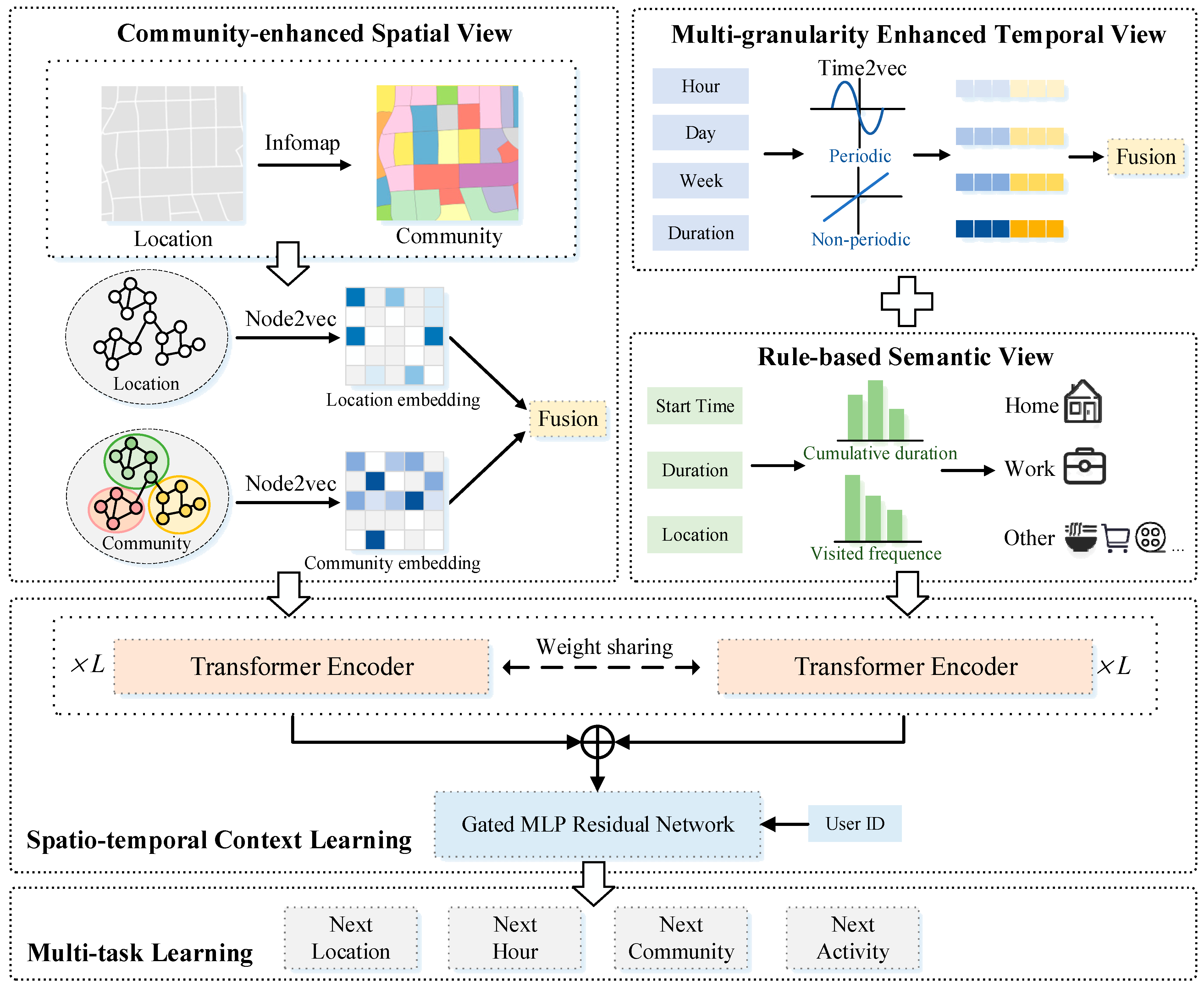
4.1. Overall Framework

Figure 2 illustrates the overall framework of the ReMVL-Net model, consisting of five components. The community-enhanced spatial view captures spatial patterns by employing community detection and graph embedding to strengthen spatial representation. The multi-granular enhanced temporal view integrates multi-granular temporal patterns and activity duration to model periodic human behaviors. Rule-based semantic view inference infers travel semantics from human mobility behavior. The spatial-temporal context learning module employs a transformer encoder to capture global contextual dependencies, while a gated residual network facilitates the integration of user features with contextual information. The multi-task learning module jointly predicts location, time, community, and activity to enhance predictive accuracy.

Figure 2. ReMVL-Net framework.

The core process of the ReMVL-Net model involves three stages. First, spatial, temporal, and semantic information are encoded using specialized heterogeneous embedding modules. In this step, temporal and semantic features are combined to form spatiotemporal semantic representations. Second, spatial and spatiotemporal semantic embeddings are fed into a transformer encoder to capture global contextual dependencies. The resulting features are then combined with user embeddings using a gated residual network to model personalized mobility patterns. Finally, a multi-task learning strategy is employed to jointly predict the next location, time, community, and activity.

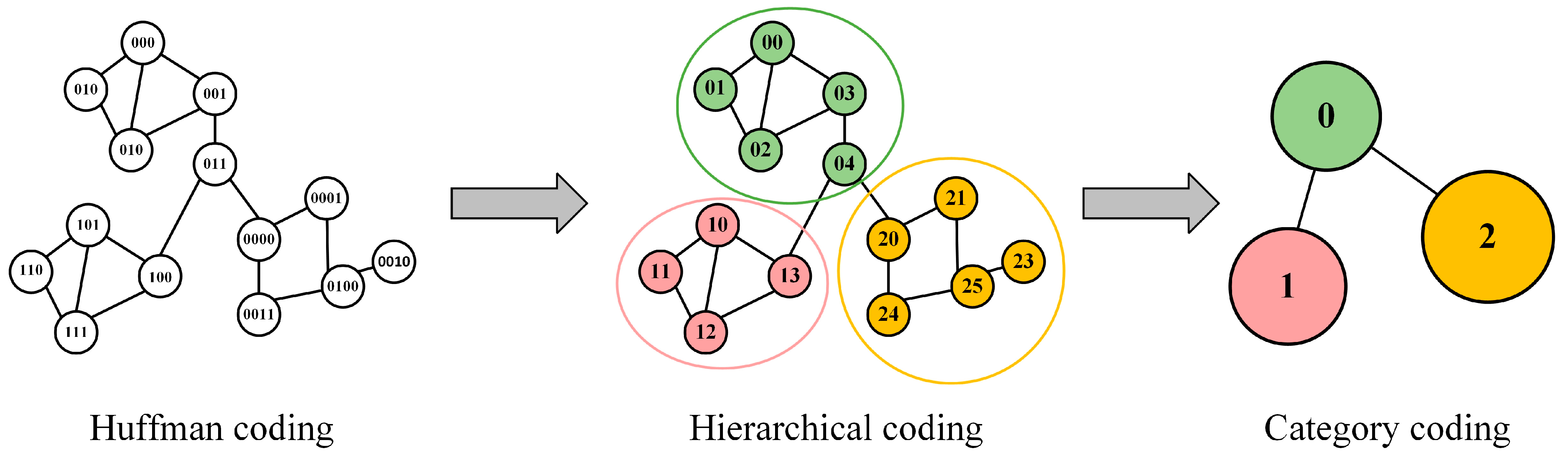
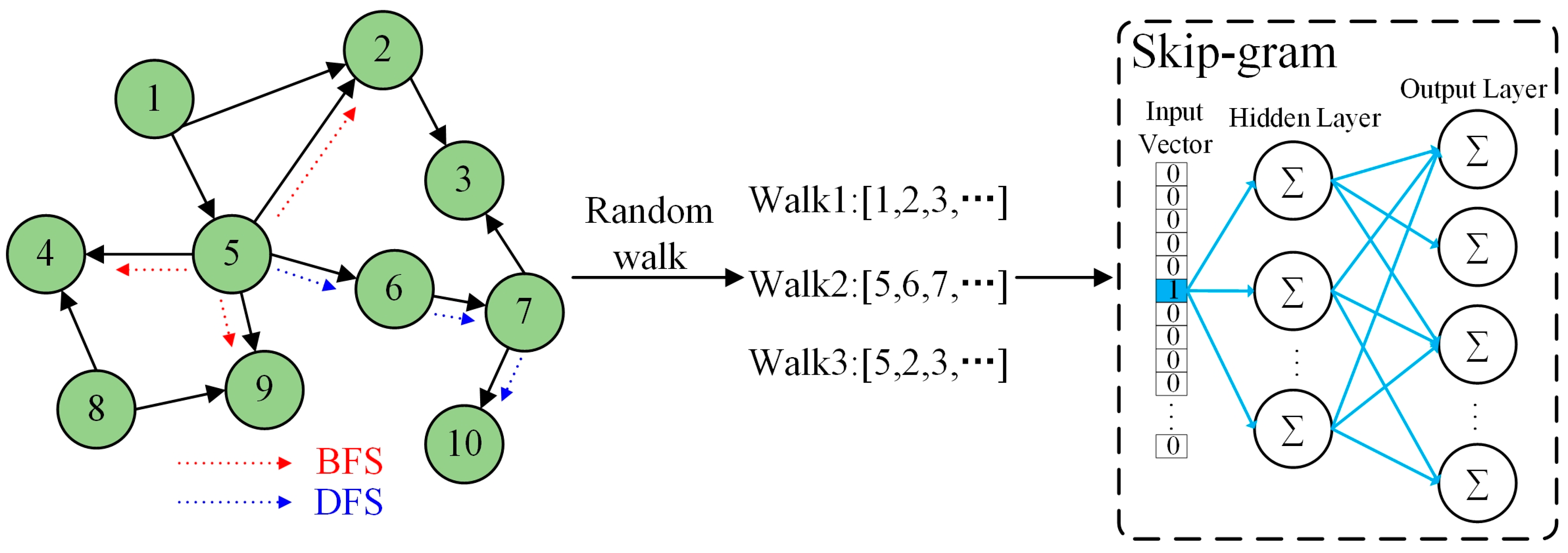
4.2. Community-Enhanced Spatial View

Human mobility typically follows stable and repetitive patterns, which are characterized by frequent movements among a limited set of locations. Previous studies often employed geographic clustering to capture human regional preferences, but this approach overlooks interaction patterns in human mobility. In contrast, community detection identifies locations with frequent interactions and groups them into communities based on the topology of the mobility network, providing a more behaviorally meaningful representation of actual mobility patterns.

From a spatial perspective, our model achieves community-enhanced spatial representation by combining community detection with graph-embedding techniques. First, community structures are extracted from user trajectories to reveal latent regional mobility patterns. Then, multi-scale spatial embeddings are generated based on both the original location transition network and the derived community-level transitions, capturing fine- and coarse-grained spatial semantics. Finally, a fusion module integrates information from different spatial levels, enabling the model to better capture individual mobility behaviors through enriched multi-scale semantic representations.

Community detection identifies locations with strong associations by analyzing group mobility patterns among location nodes. In this study, we employ the Infomap [43] algorithm to detect communities within human mobility networks. Compared with traditional modularity-based methods such as Louvain [44], Infomap naturally supports directed and weighted graphs, enabling it to capture the directional and asymmetric characteristics inherent in human mobility flows. As illustrated in Figure 3, Infomap first generates Huffman codes for all nodes based on the distribution of random walk paths. It then computes modularity, merges nodes to minimize coding length, and assigns unique codes to each community. The core optimization objective of the algorithm is to minimize the average description length required to represent a random walk path, which can be formulated as follows:

$$L\left(M\right)=q_{\curvearrowright }H\left(Q\right)+\sum _{i=1}^m{p}_{\circlearrowleft }^{i}H\left(P^i\right)$$

(1)

where $L\left(M\right)$ represents the average coding length under partition scheme $M$, and $q_{\curvearrowright }$ is the probability of exiting the current community during a random walk. $H\left(Q\right)$ denotes the information entropy of the community code, ${\mathcal{P}}^i$ is the probability of exiting community $i$, $p_{\circlearrowleft }^i$ represents the resident probability of the random walk within community $i$, and $H\left({\mathcal{P}}^i\right)$ is the information entropy of the internal movement within community $i$.

Figure 3. The process of community generation with Infomap (version 2.8.0). Numbers indicate node encoding values, while colors represent different communities.

First, we construct a directed and weighted network $G_L\left(V,E,W\right)$ based on the trajectories of all users, where $V$ denotes the set of nodes representing all locations, $E$ is the set of edges and $W$ represents the weights defined by the number of transitions between corresponding locations.

Next, the Infomap algorithm is applied to the directed and weighted location network $G_L$ to extract the set of communities $C$. Each community comprises multiple locations, and each location is assigned to a unique community (Figure 3).

Furthermore, we employ Node2vec to obtain pre-trained embedding representations of locations and communities. Proposed by Grover and Leskovec in 2016 [45], Node2vec utilizes a biased random walk strategy. Compared to one-hot encoding or conventional embedding methods, graph embedding more effectively preserves the relational structure among locations. Node2vec offers flexible control over the sampling process, enabling it to learn both local neighborhood features and global structural patterns (Figure 4).

Figure 4. Node2vec framework.

The core idea of Node2vec is to dynamically balance breadth-first search (BFS) and depth-first search (DFS) during the random walk process by introducing two adjustable parameters, $p$ and $q$, as follows:

$${\alpha }_{pq}\left(t,x\right)=\left\{\begin{array}{c}{\displaystyle \frac{1}{p}} if d_{tx}=0\\ 1 if d_{tx}=1\\ {\displaystyle \frac{1}{q}} if d_{tx}=2\end{array}\right.$$

(2)

where ${\alpha }_{pq}\left(t,x\right)$ represents the transfer probability weight from node $t$ to node $x$, and $d_{tx}$ is the shortest number of steps between the previous $t$ node and the next node $x$. Parameters $p$ and $q$ effectively capture the homophily and structural equivalence of network nodes. Specifically, the $p$ parameter influences the probability of revisiting the previous node. A higher value of $p$ makes the walk more likely to explore further nodes. The $q$ parameter controls the balance between BFS and DFS; a smaller $q$ value makes the walk more biased towards breadth-first exploration, while a larger $q$ value favors deeper exploration, guiding the walk further into the graph structure in a specific direction.

After generating node sequences via biased random walks, Node2vec treats these sequences as “sentences” and applies the skip-gram model of embedded learning to derive the final node representations, as follows:

$$n2v=Node2Vec\left(G\right)$$

(3)

Specifically, at the community level, we construct a directed and weighted network $G_C(V,E,W)$ using the same approach as that applied to the original location network. Node2vec is then applied to both the location-level and community-level transition graphs to learn the respective node embeddings. A fusion module is used to integrate the location and community embeddings into a unified multi-level spatial representation, as follows:

$$fuse=dropout\left(\sigma \left(W_{f}concat\left(H_1,H_2\right)+b_f\right)\right)$$

(4)

$$\begin{gathered} {n2v}_L=Node2Vec\left(G_L\right) \\ {n2v}_C=Node2Vec\left(G_C\right) \\ {H}_s=fuse\left({n2v}_L,{n2v}_C\right) \end{gathered}$$

(5)

where $W_f{\in R}^{2d\times d}$ is the trainable weight matrix, $b_f$ is the bias term, $d$ denotes the embedding dimension, and $H_1$ and $H_2$ represent the vectors to be fused.

4.3. Multi-Granular Enhanced Temporal View

Human mobility exhibits hierarchical temporal periodicity, which cannot be fully captured by single-granular representations. As shown in Figure 5, individuals display distinct travel patterns on weekdays and at weekends. During the day, individuals typically follow a routine of leaving in the morning and returning home at night. At a finer temporal scale, different activities may occur within the same hour, each with varying durations. To comprehensively model these multi-granular temporal dynamics of human mobility, we propose a multi-granular enhanced temporal representation.

Figure 5. Multi-granularity temporal of individual activity. The numbers indicate time encoding, and the red box highlights users’ daily commuting and short-term mobility patterns.

To capture the temporal characteristics of human mobility at multiple scales, we divide time into three granular levels. At the hour level, each hour is subdivided into four 15 min intervals to reflect short-term activity transitions. At the day level, a 24 h encoding scheme is employed to model daily periodic patterns. At the week level, temporal information is encoded using the week number to represent long-term weekly regularities. In addition to these discrete temporal features, duration is incorporated as a supplementary attribute to describe the length of stay.

To further enhance the representation of temporal information, we employ Time2vec [46], a time encoding model that captures both periodic and linear temporal patterns via a combination of sinusoidal and linear functions. This enriched encoding enables the model to better learn complex time-dependent behaviors across multiple temporal granularities and durations. Time2vec is defined as follows:

$$t2v\left(\tau \right)\left[i\right]=\left\{\begin{array}{l}{\omega }_i\tau +{\phi }_i, if i=0.\\ \mathcal{F}\left({\omega }_i\tau +{\phi }_i\right), if 1\le i\le k.\end{array}\right.$$

(6)

where $k$ represents the dimension of Time2vec, $\mathcal{F}$ is the periodic activation function, which can be either a sine or cosine function, and ${\omega }_i$ and ${\phi }_i$ are learnable parameters.

By integrating the multi-granular temporal information, we obtain a joint embedding representation for the temporal view. The integration strategy is described as follows:

$$\begin{gathered} H_t=fuse\left(t2v\left(day\right),t2v\left(hour\right)\right) \\ {H}_t^{\prime }=fuse\left(H_t,t2v\left(week\right)\right) \\ {H}_t^{″}=fuse\left(H_t^{\prime },t2v\left(duration\right)\right) \end{gathered}$$

(7)

4.4. Rule-Based Semantic View

Accurate identification of travel semantics can enhance the model’s understanding of human mobility behavior. However, location semantics may be ambiguous, as different individuals can have varying travel purposes at the same place. To address this challenge, we propose a rule-based travel semantic recognition mechanism (Figure 6). This mechanism infers location semantics by analyzing individuals’ visit frequency, duration of stay, and visit timing across different locations.

Figure 6. Rule-based travel semantic recognition mechanism.

Human mobility patterns typically involve frequent visits to a limited number of locations, with home and workplace forming the core of regular movement [47,48]. Other activities, such as dining and entertainment, are generally constrained by the locations of home and work. Therefore, we categorize user mobility semantics into three types: home, work, and other. Specifically, for each individual, the location with the longest cumulative stay during nighttime hours is labeled as home. Among the remaining locations, the one with the highest historical visit frequency is assigned as the work location. In contrast, visits to other activity locations are far less frequent and highly dispersed. Following previous studies [49], we classify locations outside of home and work as other social activities, rather than introducing finer-grained categories. Through user-level semantic labeling, each location may carry different meanings for different individuals. For example, a spatial unit may serve as home for user A, while for user B, it may represent an occasionally visited other location. Finally, we employ the embedding method to embed the travel semantics:

$$H_{Act}=Embedding\left(act\right)$$

(8)

We integrate the temporal view and semantic view into a spatiotemporal semantic module. This design is grounded in previous research demonstrating a significant correlation between time and travel activities [41].

4.5. Spatiotemporal Context Learning

We utilize a transformer encoder [50] to learn the spatiotemporal context. The encoder comprises multi-head self-attention layers, a feed-forward neural network, and residual connections with layer normalization. We designed two transformer encoders: one for modeling spatial features and another for spatiotemporal semantic features. These encoders share weights to reduce model complexity and enhance generalization. To capture individual differences in mobility, we incorporate user ID embeddings, enabling the model to learn personalized mobility patterns and improve prediction accuracy for each user.

Finally, the spatial features, spatiotemporal semantic features, and user information are combined into a joint representation through the following summation:

$$X=trans\left(H_s\right)+trans\left(H_{A,t}\right)+Embedding\left(ID\right)$$

(9)

To effectively integrate personalized information with spatiotemporal context and enhance the model’s capacity to learn personalized patterns, we propose a gated MLP residual network (Figure 7). In this structure, a multilayer perceptron (MLP) is used to project and transform the input features into a unified representation space, thereby facilitating the fusion of user-specific and contextual information. The gating mechanism within the gated MLP regulates the information flow through a gating mechanism, allowing the model to adaptively emphasize relevant features. Residual connections and layer normalization are incorporated to enhance generalization and training stability. The gated MLP residual network is defined as follows:

$$\begin{array}{c}\begin{array}{c}{X}_{Gate}=W_{g3}\left(W_{g1}X+b_{g1}\right)·\sigma \left(W_{g2}X+b_{g2}\right)+b_{g3}\\ X_{Gate}^{\prime }=LayerNorm\left(X+{Dropout(X}_{Gate}\right))\end{array}\end{array}$$

(10)

where $W_{g1}$, $W_{g1}$, and $W_{g3}$ are the learnable weight matrices, $b_{g1}$, $b_{g2}$, and $b_{g3}$ are the bias terms, $LayerNorm$ is layer normalization applied across the feature dimension, and $Dropout$ is used to randomly zero out inputs for regularization.

Figure 7. Gated MLP Residual Network. LeakyReLU is used as the activation function.

4.6. Multi-Task Learning

Finally, we employ a multi-task learning strategy to jointly optimize four objectives: location prediction, community prediction, time prediction, and activity prediction. The outputs for each task are computed as follows:

$$\begin{array}{c}{Y}_{Loc}=W_{Loc}{X}_{Gate}^{\prime }+b_{Loc}\\ Y_{Com}=W_{Com}{X}_{Gate}^{\prime }+b_{Com}\\ Y_{Time}=W_{Time}{X}_{Gate}^{\prime }+b_{Time}\\ Y_{Act}=W_{Act}{X}_{Gate}^{\prime }+b_{Act}\end{array}$$

(11)

where $W_{Loc}\in R^{d\times N_{loc}}$, $W_{Com}\in R^{d\times N_{com}}$, $W_{Time}\in R^{d\times N_{time}}$, and $W_{Act}\in R^{d\times N_{act}}$ are the learnable weight matrices, and $b_{Loc}$, $b_{Com}$, $b_{Time}$, and $b_{Act}$ are the bias terms.

The model employs the cross-entropy loss for each task. The overall loss is defined as the sum of the individual task losses, as follows:

$$\mathcal{L}={\mathcal{L}}_{Loc}+{\mathcal{L}}_{Com}+{\mathcal{L}}_{Time}+{\mathcal{L}}_{Act}$$

(12)

where ${\mathcal{L}}_{Loc}$, ${\mathcal{L}}_{Com}$, ${\mathcal{L}}_{Time}$ and ${\mathcal{L}}_{Act}$ represent the cross-entropy losses for location prediction, community prediction, time prediction, and activity prediction, respectively.

5. Experiment and Analysis

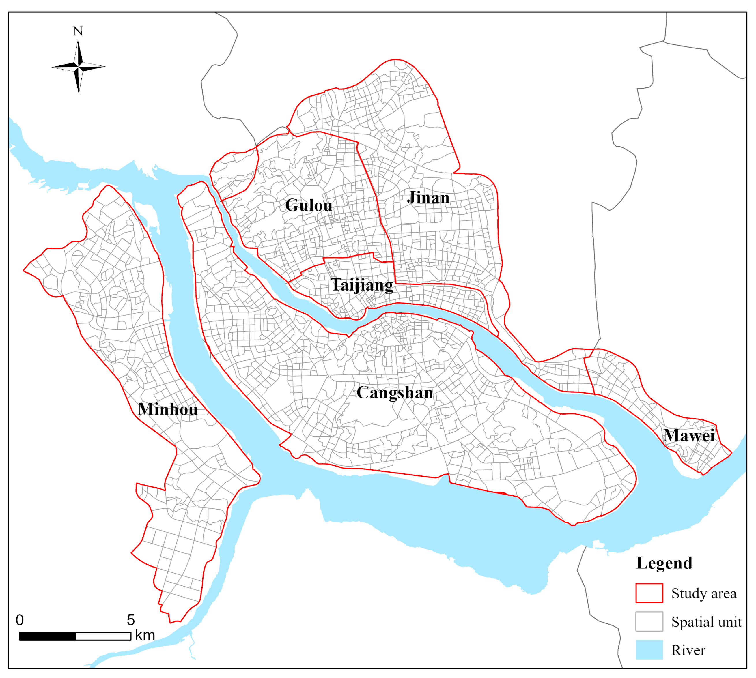
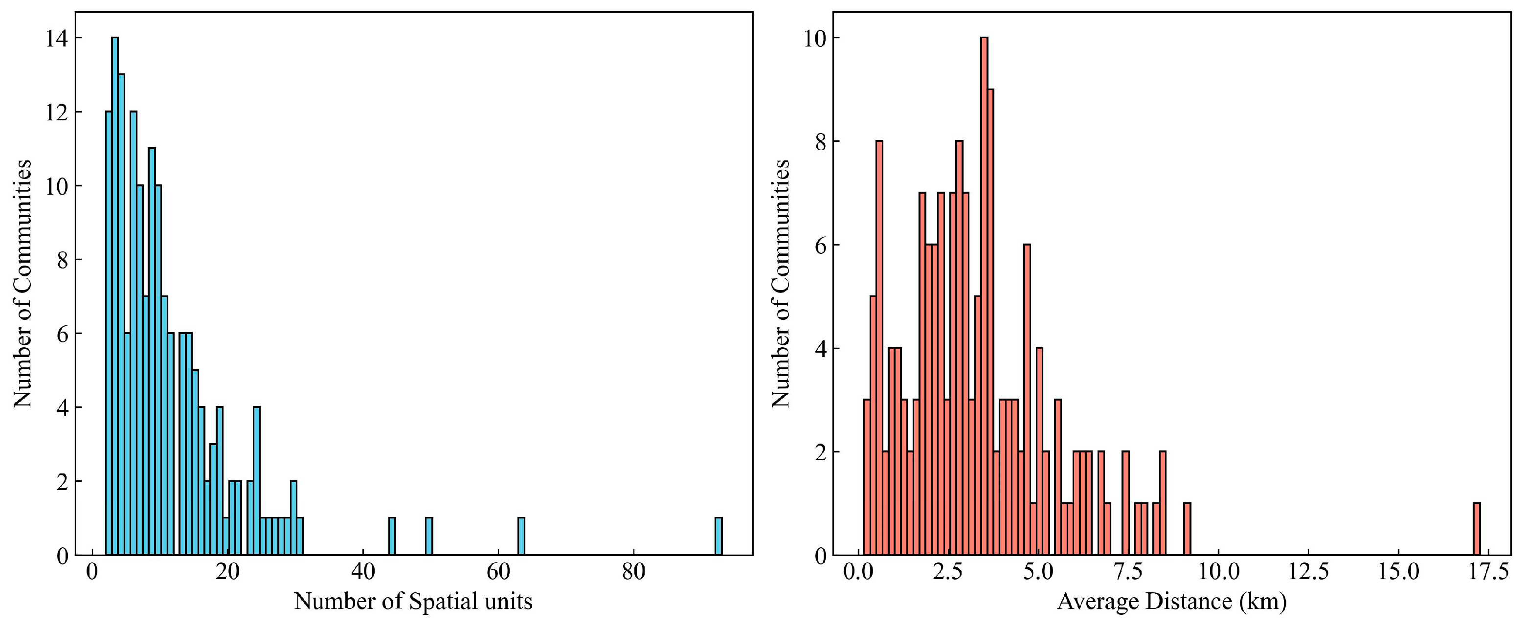
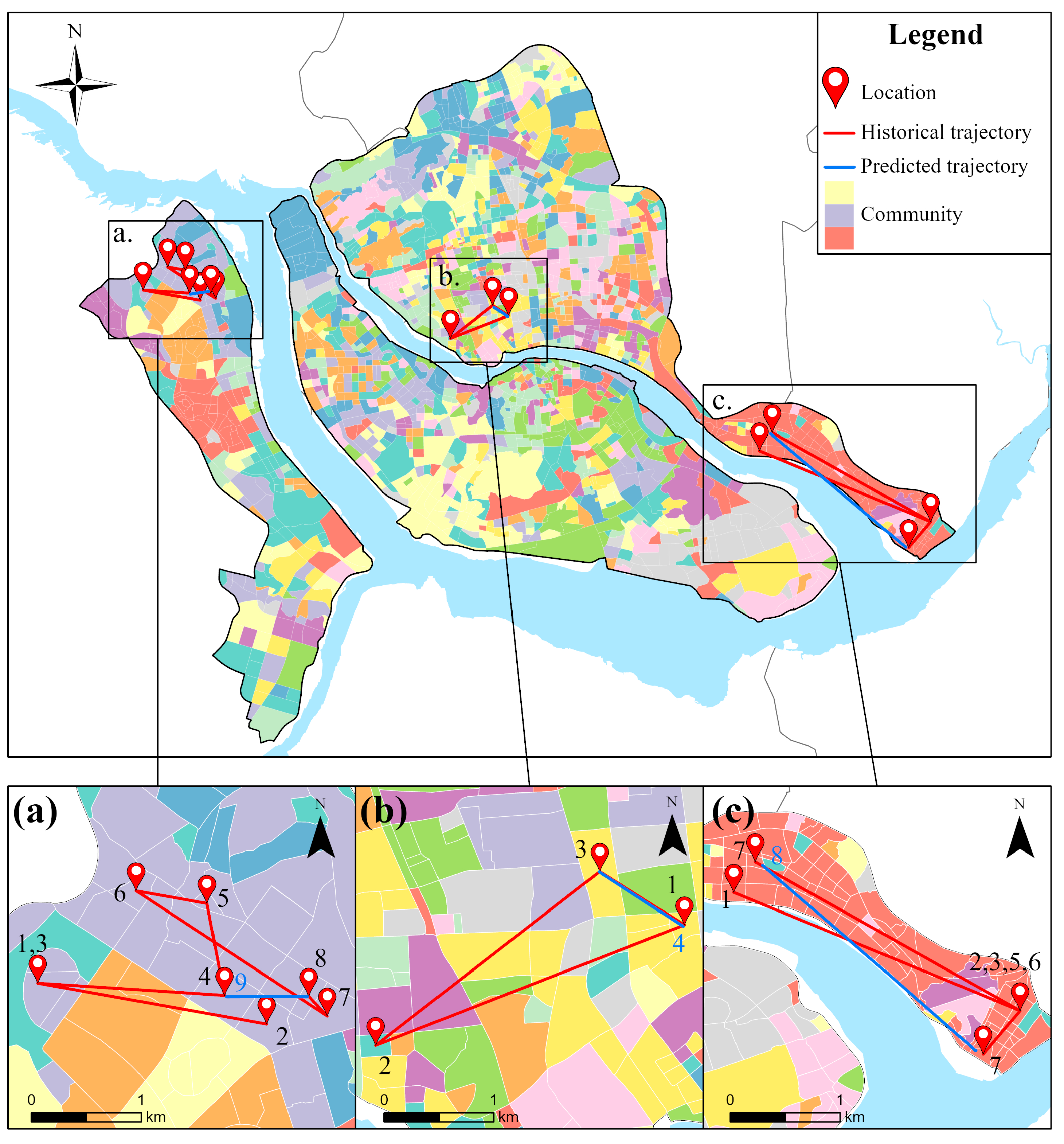
5.1. Study Area and Data

The research area was located in the main urban area of Fuzhou (Figure 8), which lies on the southeast coast of China. Fuzhou, the capital of Fujian Province, governs six districts, six counties, and one county-level city.

Figure 8. The study area and spatial units.

Spatial discretization is a crucial preprocessing step for location prediction using GNSS datasets. Existing studies commonly partition spatial units using regular grids [51], base station areas [42], or clustering algorithms [21]. However, these approaches may fragment continuous urban structures, resulting in semantic inconsistencies. In practice, human mobility behavior is shaped by the urban built environment, including the road network, water systems, and natural landscapes, which inherently segment the city into regions of varying sizes. Therefore, we utilized OpenStreetMap (OSM) road network data to define the spatial units of the study area (Figure 8). The spatial units exhibit size variation, with a maximum area of 3.49 km² and an average area of 0.15 km².

The timing dataset used in this study was provided by a location service company and originated from GNSS location data collected via mobile phones. The dataset covered mobile users in Fuzhou during March 2023. Each record contained a user ID, timestamp, longitude, and latitude (Table 1). To address privacy concerns, all user identifiers were anonymized. In our study, all user IDs have been anonymized to safeguard privacy. In the data preprocessing stage, we first excluded users with fewer than 10 location records per day on average. Then, 1500 users were randomly sampled from the remaining dataset. During trajectory generation, we used a 7-day sliding window and excluded those with fewer than three valid trajectories within each window. As a result, the final dataset comprised 1208 users with sufficiently complete trajectories.

Table 1. Example of Timing data.

User ID	Longitude	Latitude
0000269a***292c0c	119.30889	26.112497
00007ebc***5cdc7c	119.18924	26.068150
…	…	…
00002edc***8ef30a	119.25607	26.109436

Stay points were identified following the method proposed by Ye et al. [52] As illustrated in Figure 9, the method extracts stay points by identifying segments in a trajectory where the user remains within a small spatial range for a sustained period. To determine appropriate thresholds for stay point detection, we first analyzed the distributions of temporal and spatial intervals between consecutive records (Figure 10). The results indicate that approximately 75% of transitions occurred within 200 m and 45 min. Based on this empirical distribution, we set the distance and time thresholds to 200 m and 45 min, respectively. After identifying stay points, a total of 1208 users generated 148,518 stay point records.

Figure 9. Stay point recognition.

Figure 10. Distributions of temporal and spatial intervals.

Furthermore, we also conducted a statistical analysis of users’ stay behaviors. In Figure 11, the left panel displays the number of unique locations visited by each user. Most users visited fewer than 40 distinct locations. As shown in the right panel of Figure 11, we calculated the average visit probability across all users, based on the ranked frequency of locations. The two most frequently visited locations accounted for 68% of total visits. This finding aligns with previous studies [47], indicating that users’ daily mobility is typically confined to a limited set of locations, reflecting regular and habitual activity patterns.

Figure 11. Statistical analysis of users’ stay behaviors. The left panel presents the distribution of the number of unique locations visited per user. The right panel illustrates the average visit probability for locations, ranked by visit frequency.

For dataset partitioning, an 8:1:1 ratio was used, with the first 24 days allocated for training, the next 4 days for validation, and the final 3 days for testing. Regarding trajectory length, user trajectories were segmented using a sliding window with a 2-day window size, where the last position of each trajectory served as the prediction label. To ensure consistent trajectory lengths within each batch, shorter trajectories were padded with zeros to match the maximum length within the batch.

5.2. Comparison of Models

We conducted comparative experiments between the proposed model and two categories of baseline models, classical location prediction methods and multi-view location prediction models, as follows:

• Markov: This method treats locations as states and constructs a transition probability matrix to describe state transitions. It is a fundamental approach in location prediction;
• RNN: RNN utilizes the output of the previous time step as the input for the current time step, making it well suited for modeling sequential data. It is a widely used deep learning method;
• SERM [32]: Built on the LSTM framework, SERM integrates embeddings of location, temporal, semantics, and user ID to achieve multi-dimensional feature fusion;
• MSSRM [40]: This model enhances location prediction by combining LSTM with self-attention mechanisms. It employs Time2vec and Node2vec to embed temporal and spatial information, improving representation capability;
• MUPT [34]: This model leverages GGNN to learn expressive POI embeddings from a global trajectory graph and uses three dedicated transformer encoders to model temporal, categorical, and sequential user preferences;
• GetNext [33]: This model integrates a graph-enhanced transformer with global trajectory flow modeling. It fuses user preferences, spatiotemporal contexts, and time-aware category embeddings to capture collaborative signals across users;
• MHSA [21]: Based on the multi-head self-attention mechanism, MHSA learns location transition patterns from historical visits, multi-scale temporal features, activity duration, and surrounding land use, facilitating accurate location inference.

5.3. Evaluation Indicators

In this study, we evaluate the model’s performance using three commonly used metrics in location prediction. The evaluation indicators are as follows:

• Accuracy: Accuracy measures the agreement between the predicted and actual locations. In this study, Acc@K is used to represent the model’s prediction accuracy. Specifically, the model outputs a probability distribution over candidate locations, which is ranked in descending order. Acc@K determines whether the true location appears within the top K predictions. Acc@1 indicates whether the location with the highest probability is correct, while Acc@5 and Acc@10 assess whether the true location is included among the top five and top ten predictions, respectively. The accuracy is computed using the following formula:

  $$Acc@k={\displaystyle \frac{1}{N}}\sum _{i=1}^N\mathbb{I}\left(y_i\in {\widehat{Y}}_i^k\right)$$

  (13)

  where $N$ represents the total number of test samples, $y_i$ denotes the actual location of the $i$ sample, and ${\widehat{Y}}_i^k$ is the set of the top $k$ predicted candidate locations for the $i$ sample. The indicator function $\mathbb{I}$ returns 1 if $y_i$ is included in ${\widehat{Y}}_i^k$, and 0 otherwise;
• Mean Reciprocal Rank (MRR): MRR measures the average of the reciprocal ranks of the correct predictions within the candidate outcomes. It evaluates the relative ranking of the actual location among the top K predicted results. A higher MRR value indicates a more accurate prediction. The calculation formula is as follows:

  $$MRR={\displaystyle \frac{1}{N}}\sum _{i=1}^N{\displaystyle \frac{1}{{rank}_i}}$$

  (14)

  where ${rank}_i$ represents the position of the true location for the $i$ sample within the predicted candidate list;
• Normalized Discount Cumulative Gain (NDCG): NDCG evaluates both the relevance and ranking of predicted results. It first calculates the discounted cumulative gain (DCG) by applying a discount factor to the relevance score of each predicted outcome, reducing the influence of lower-ranked results. The DCG is then normalized using the ideal discounted cumulative gain (IDCG) to obtain the NDCG value, which ranges from 0 to 1. A value closer to 1 indicates better model performance. NDCG effectively captures the ranking capability of the model and the relevance of its predictions. The calculation formula is as follows:

  $$NDCG@k={\displaystyle \frac{DCG@k}{IDCG@k}}$$

  (15)

  where $NDCG@k$ evaluates the ranking quality of the model based on the top K predicted positions. In this study, NDCG@10 is used as the evaluation metric.

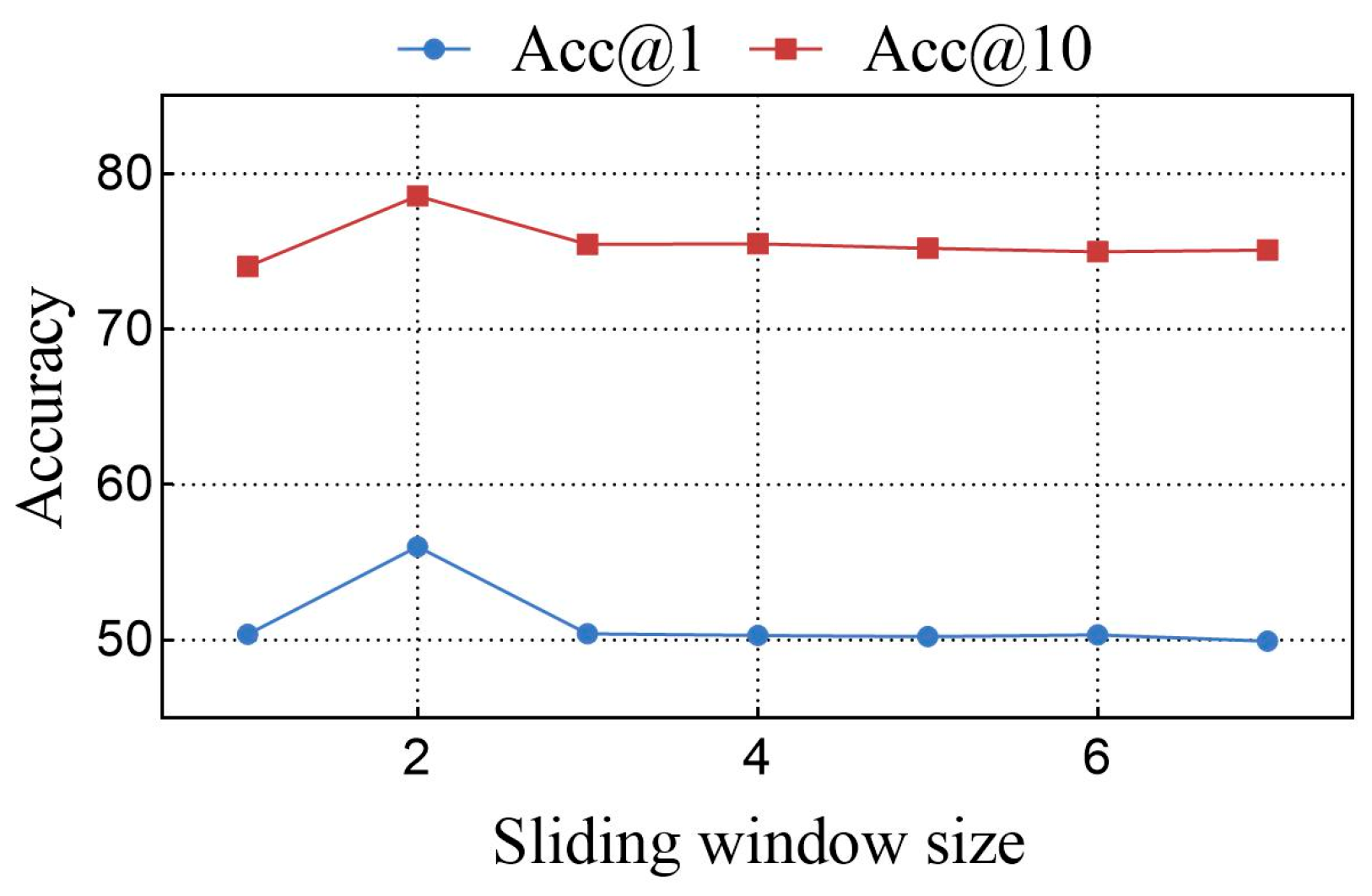
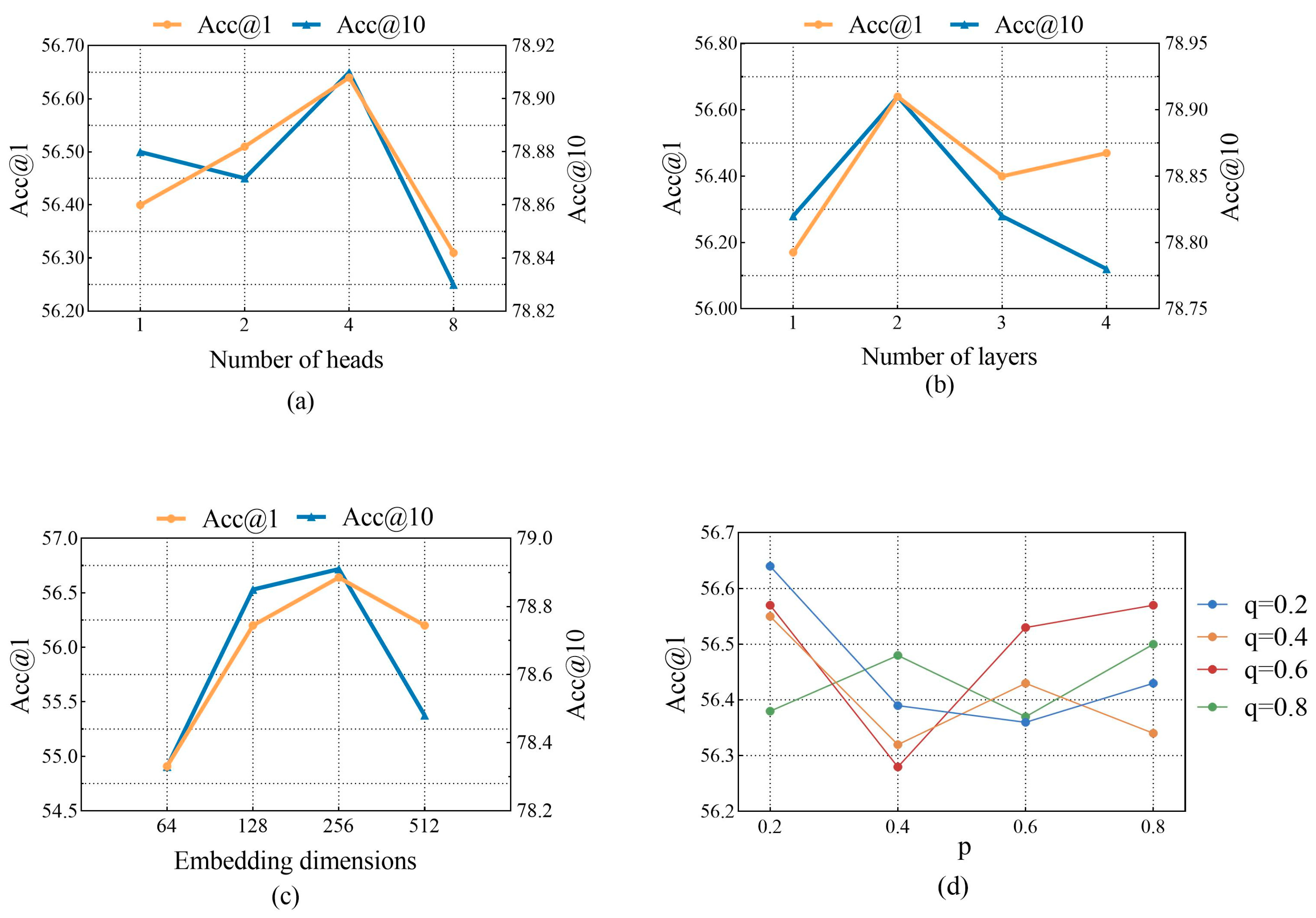
5.4. Hyperparameter Experiment

The Adam optimizer was used for model training in this experiment. The learning rate was set to 0.002, and the weight decay coefficient was set to 0.0001. The batch size was 1024, and the feature embedding dimension was set to 256. The transformer encoder consisted of two stacked layers, each with four attention heads. The feedforward neural network had a hidden layer dimension of 256. The fusion module employed a dropout rate of 0.3, while the residual module had a dropout rate of 0.2. For community detection, we used Infomap version 2.8.0 with the —two-level and —directed options. In addition, Node2vec version 0.5.0 was used. The hardware configuration included an NVIDIA RTX 3060 GPU and an AMD Ryzen 7 6800H CPU.

We first evaluated how the length of the sliding time window affected the model performance (Figure 12). A range of window sizes from 1 to 7 days was tested. The model achieved its highest accuracy with a 2-day window, while performance gradually decreases with longer windows. Based on these results, we selected 2 days as the optimal window length for trajectory segmentation.

Figure 12. Impact of sliding window size on model performance.

Additionally, we evaluated the impact of the following four key hyperparameters on model performance: the number of attention heads, the number of encoder layers, the dimension of the embedding layers, and the impact of parameters p and q in Node2vec.

As shown in Figure 13, increasing the number of attention heads initially enhanced model performance, indicating that multi-head attention was more effective in capturing complex patterns than single-head attention. The model achieved optimal performance when the number of heads was set to four. However, further increasing the number of heads resulted in performance degradation and overfitting. A similar trend was observed with respect to the number of encoder layers, where the best results were obtained with two layers.

Figure 13. Effect of different hyperparameters on model performance. (a) Impact of attention head; (b) Impact of encoder layer; (c) Impact of embedding layer; (d) Impact of parameters p and q in Node2vec.

The embedding dimension also has a substantial influence on model performance. A smaller dimension constrains the model’s capacity to learn complex features, while a larger dimension improves representational capability. However, overly large dimensions may introduce overfitting. The experimental results demonstrate that an embedding dimension of 256 yielded the best performance.

For the Node2vec hyperparameters p and q, we conducted experiments with values ranging from 0.2 to 0.8. The results show that the best performance was achieved when both p and q were set to 0.2.

5.5. Performance Evaluation of Next Location Prediction

Table 2 presents the experimental results. Each experiment was independently repeated five times, and the mean and standard deviation for each metric were calculated. The best results are highlighted in bold, while the second-best results are underlined. We performed paired t-tests between our model and baselines, confirming that the improvements were statistically significant at p < 0.05. The analysis shows that the proposed model outperformed all baseline models. Compared with the MHSA model, the proposed model achieved improvements of 2.94% in Acc@1, 0.88% in Acc@5, 1.14% in Acc@10, 2.41% in MRR, and 2.22% in NDCG@10.

Table 2. Performance comparison for next location prediction.

Model	Acc@1	Acc@5	Acc@10	MRR	NDCG@10
Markov	42.30	59.11	61.14	49.59	52.40
RNN	46.64 ± 0.23	69.32 ± 0.25	73.90 ± 0.15	56.97 ± 0.18	60.75 ± 0.18
SERM	50.65 ± 0.16	73.76 ± 0.21	77.50 ± 0.21	60.97 ± 0.05	64.77 ± 0.06
MSSRM	53.73 ± 0.12	73.51 ± 0.13	77.42 ± 0.14	62.70 ± 0.10	66.00 ± 0.09
MUPT	53.72 ± 0.25	72.34 ± 0.07	75.86 ± 0.17	62.20 ± 0.16	65.26 ± 0.15
MHSA	53.86 ± 0.10	74.16 ± 0.24	78.02 ± 0.13	62.94 ± 0.08	66.36 ± 0.05
GetNext	55.02 ± 0.18	73.41 ± 0.15	77.62 ± 0.09	63.37 ± 0.08	66.53 ± 0.06
ReMVL-Net	56.64 ± 0.14	74.82 ± 0.07	78.91 ± 0.18	64.90 ± 0.11	68.01 ± 0.12

The best results are highlighted in bold, while the second-best results are underlined.

Among the baseline models, the Markov model performed significantly worse than deep learning-based methods, as it relies solely on the current location to predict the next one and fails to incorporate historical contextual information. The RNN achieved better performance by utilizing both the hidden state and temporal dependencies from previous steps. However, both the Markov and RNN models depend exclusively on the original location sequence, resulting in inferior performance compared with multi-view models.

The SERM model integrates location, temporal, and semantic features, and employs LSTM to address the limitations of RNNs in modeling long-term dependencies, thereby achieving strong results. The MSSRM model enhances prediction by leveraging Node2vec and Time2vec for spatiotemporal embedding, while applying self-attention mechanisms within the LSTM framework to extract local features, leading to notable improvements in Acc@1. The GetNext model further improves performance by jointly modeling global trajectory flows, temporal contexts, and activity semantics, ranking second in terms of Acc@1. However, these models lack the capability to capture human mobility patterns across multiple spatial scales, which constrains their performance and leads to lower accuracy compared with the proposed method.

5.6. The Influence of Model Components

To evaluate the contribution of each core module, we conducted ablation experiments by modifying or removing key components of the proposed model. First, we replaced the transformer encoder with an LSTM to assess the impact of the self-attention mechanism on capturing long-range dependencies in mobility patterns. Second, we removed the gated MLP residual network, which is responsible for fusing multi-view features, to evaluate its effectiveness in integrating heterogeneous representations. Third, we replaced the spatial and temporal encoding modules individually by substituting Node2vec and Time2vec with standard trainable embedding layers, in order to examine their specific roles in capturing structural spatial relationships and periodic temporal dynamics.

As shown in Table 3, replacing the transformer with an LSTM led to a noticeable reduction in prediction accuracy, indicating that the self-attention mechanism offers a stronger capacity for modeling long-range dependencies in human mobility sequences. The gated MLP module further enhances the model by enabling more effective integration of heterogeneous features. Moreover, Node2vec and Time2vec enhance the spatial and temporal representations, respectively, thereby contributing to the model’s overall accuracy.

Table 3. Ablation study of the model components.

Model	Acc@1	Acc@5	Acc@10	MRR	NDCG@10
Full	56.64 ± 0.14	74.82 ± 0.07	78.91 ± 0.18	64.90 ± 0.11	68.01 ± 0.12
w/o Transformer	56.17 ± 0.08	74.62 ± 0.10	78.54 ± 0.17	64.55 ± 0.08	67.67 ± 0.10
w/o Gated MLP	52.59 ± 0.36	71.93 ± 0.26	76.18 ± 0.11	61.49 ± 0.29	64.70 ± 0.24
w/o Node2vec	56.27 ± 0.08	74.75 ± 0.08	78.73 ± 0.14	64.68 ± 0.07	67.81 ± 0.09
w/o Time2vec	56.31 ± 0.18	74.70 ± 0.13	78.71 ± 0.16	64.68 ± 0.12	67.80 ± 0.12

The best results are highlighted in bold, while the second-best results are underlined.

5.7. The Influence of Multi-Task Learning

To evaluate the effectiveness of the multi-task learning framework, we conducted ablation experiments on time, activity, and community prediction tasks. The results are presented in Table 4. As shown, the multi-task learning framework contributed positively to improving the model’s prediction accuracy. Time prediction plays a significant role in enhancing the overall performance. In particular, the community prediction task had a greater impact on Acc@5 and Acc@10 compared to other tasks, indicating that community prediction is effective in narrowing the candidate space for next-location prediction.

Table 4. Ablation study of the multi-task learning.

Model	Acc@1	Acc@5	Acc@10	MRR	NDCG@10
Full	56.64 ± 0.14	74.82 ± 0.07	78.91 ± 0.18	64.90 ± 0.11	68.01 ± 0.12
w/o Time	55.05 ± 0.10	74.80 ± 0.15	78.89 ± 0.07	64.01 ± 0.08	67.36 ± 0.08
w/o Act	56.20 ± 0.23	74.78 ± 0.16	78.85 ± 0.10	64.67 ± 0.13	67.82 ± 0.10
w/o Com	56.44 ± 0.14	74.61 ± 0.04	78.84 ± 0.12	64.73 ± 0.11	67.87 ± 0.11

The best results are highlighted in bold, while the second-best results are underlined.

5.8. The Influence of Spatiotemporal Context

To evaluate the influence of spatiotemporal context on model performance, we designed seven ablation experiments by selectively removing specific features, as follows: (1) without temporal week granularity; (2) without temporal day granularity; (3) without temporal hour granularity; (4) without duration of individual stays; (5) without travel activity; (6) without community information; (7) without user ID.

The ablation results are presented in Table 5. The results demonstrate that excluding any of these features led to a decline in model performance, confirming their importance.

Table 5. Ablation study of the spatiotemporal context.

Model	Acc@1	Acc@5	Acc@10	MRR	NDCG@10
Full	56.64 ± 0.14	74.82 ± 0.07	78.91 ± 0.18	64.90 ± 0.11	68.01 ± 0.12
w/o Week	56.51 ± 0.18	74.65 ± 0.10	78.80 ± 0.10	64.80 ± 0.12	67.91 ± 0.07
w/o Day	53.53 ± 0.16	74.30 ± 0.08	78.64 ± 0.14	62.92 ± 0.08	66.44 ± 0.09
w/o Hour	56.38 ± 0.12	74.79 ± 0.03	78.83 ± 0.11	64.75 ± 0.06	67.88 ± 0.04
w/o Duration	53.58 ± 0.09	74.46 ± 0.19	78.67 ± 0.10	63.03 ± 0.06	66.55 ± 0.07
w/o Act	55.83 ± 0.08	74.71 ± 0.10	78.75 ± 0.09	64.45 ± 0.06	67.63 ± 0.06
w/o Com	55.68 ± 0.15	74.09 ± 0.24	78.26 ± 0.24	64.06 ± 0.14	67.20 ± 0.17
w/o User	52.79 ± 0.15	71.79 ± 0.20	76.04 ± 0.21	61.47 ± 0.16	64.65 ± 0.18

The best results are highlighted in bold, while the second-best results are underlined.

5.8.1. Influence of Community

Community features had a more significant impact on Acc@5 and Acc@10 compared to temporal and activity information, suggesting that they effectively reduced the candidate location set.

A total of 161 communities were detected in the experiment. As shown in Figure 14, most communities contained fewer than 20 spatial units. The average internal distance between spatial units within communities was 3.56 km. Approximately 70% of communities exhibited an average internal spatial unit distance of around 4 km, indicating a certain degree of spatial continuity.

Figure 14. Community detection results. The left panel shows the number of spatial units contained in different communities. The right panel shows the average internal distance of spatial units within different communities.

The prediction results are visualized in Figure 15, displaying the historical trajectories and predicted locations of three users. The historical locations are sequentially numbered, with historical trajectories marked in red and predicted trajectories marked in blue. It can be observed that most of the users’ locations fall within the same communities. Notably, the communities are not entirely continuous, indicating that community detection relies on individuals’ mobility patterns and successfully identifies their preferred activity areas.

Figure 15. The trajectories of three users. Panels (a–c) show the trajectories of three different users, where the numbers indicate the sequential order of movements.

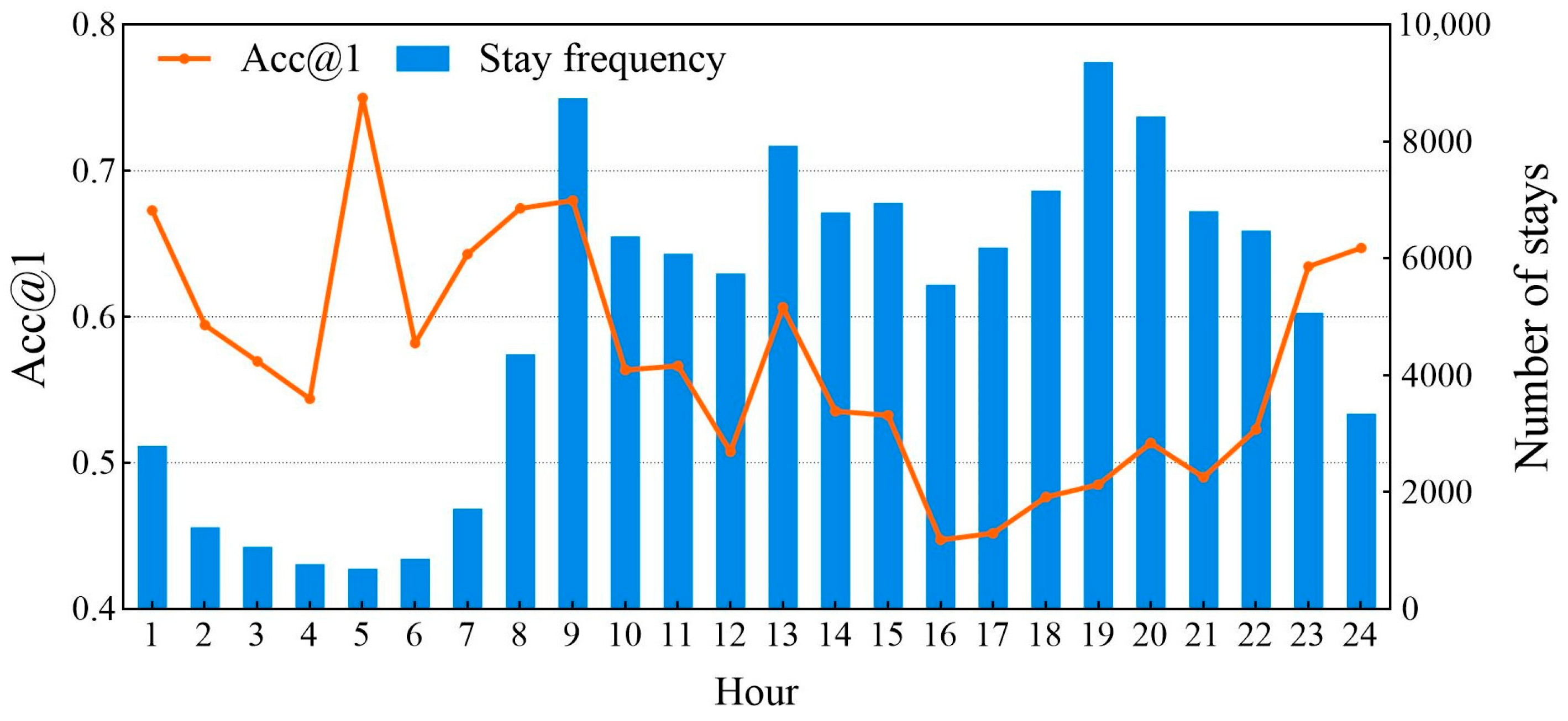
5.8.2. Influence of Temporal Features

From a temporal perspective, the influence of temporal features varies across different scales, with the temporal day-granularity feature having the most significant impact. Specifically, removing the daily temporal feature resulted in a significant decline in Acc@1, highlighting the strong regularity of human mobility behavior within a single day. Figure 16 illustrates the fluctuations in human flow and prediction accuracy throughout the day. Notably, prediction accuracy shows considerable variation, with the highest accuracy occurring during the late-night hours, particularly between 4 and 5 a.m., when most individuals are typically at home. Conversely, prediction accuracy is lowest between 3 and 8 p.m., coinciding with peak human flow, suggesting that individuals’ mobility behaviors become more diverse in the afternoon and evening.

Figure 16. Acc@1 and human mobility fluctuations over time.

In contrast, the impact of the temporal week-granularity feature is relatively small. This may be attributed to the smoother variations in individuals’ mobility patterns on a weekly scale, which result in a less pronounced effect on model performance compared to the daily scale. Figure 17 presents the variation in activity frequency throughout the week, showing notable differences between weekdays and weekends. On weekdays, activity peaks typically occur in the morning, midday, and evening, reflecting a regular commuting pattern. In contrast, on weekends, the peak activity frequency shifts to 6–7 p.m., likely due to leisure activities. The peak frequency on weekdays is higher than on weekends, indicating a more concentrated and frequent travel demand during the weekdays. Furthermore, the temporal hour-granularity feature also exerts some influence on the model, suggesting that fine-grained temporal patterns are valuable for improving location prediction.

Figure 17. Heatmap of weekly activity frequency.

5.8.3. Influence of Travel Semantics

Travel semantics play a crucial role in helping the model accurately predict the most likely next location. As shown in Figure 18, the two primary activity semantics, home and work, accounted for 39.36% and 33.81% of users’ total stay activities, respectively. Together, these activities accounted for 73% of total stay behaviors, indicating that home and work activities dominate most of users’ daily routines and highlighting the significant regularity in human mobility patterns. The remaining 27%, categorized as other social activities, reflects the diversity of human movements. This portion is often more variable in nature, introducing greater uncertainty to location prediction tasks. Figure 19 illustrates the prediction accuracy of travel activities across different time segments of the day, which are divided into five periods: morning (7:00–11:00), noon (11:00–14:00), afternoon (14:00–18:00), evening (18:00–23:00), and late night (23:00–7:00). The prediction accuracy varies across the three activities, with home and work activities, which exhibit significant spatiotemporal regularities, demonstrating higher predictability. Conversely, other social activities exhibit lower prediction accuracy. From a temporal perspective, home activities exhibit the highest prediction accuracy during the night, while work activities show peak accuracy in the morning, with the lowest accuracy in the evening. This pattern is closely linked to individuals’ commuting behaviors. Other social activities show relatively higher prediction accuracy during the noon and afternoon periods, with the lowest accuracy observed during the evening hours. This reflects the greater randomness and variability of non-commuting activities, highlighting the diverse nature of urban lifestyles beyond routine commuting [42].

Figure 18. Proportions of three activities.

Figure 19. Acc@1 of the three activity types across five time periods, with 95% confidence intervals.

5.8.4. Influence of Individual

After removing the user-embedding module, there was a significant decrease in model accuracy, indicating that user embedding had the greatest impact on model performance among all features. To further explore this, we analyzed the relationship between the number of different locations visited by individuals and the prediction accuracy. As shown in Figure 20, there was an inverse correlation between the number of different locations visited by users and prediction accuracy. This suggests that individuals with more diverse mobility behaviors, who visit a greater number of locations, present greater challenges for mobility prediction. In contrast, individuals with simpler mobility patterns, visiting fewer locations, exhibit more predictable behavior [21]. By embedding the user ID, the model is better able to identify and distinguish the mobility of different individuals, thereby enhancing its ability to make personalized predictions.

Figure 20. Relationship between prediction accuracy and the number of different locations visited.

6. Discussion and Conclusions

To address the limitations of existing research in capturing the spatiotemporal context of human mobility, this paper proposes a ReMVL-Net model designed to more accurately capture complex human mobility patterns. We conducted experiments on the timing dataset, and the results show that our proposed model outperformed the comparison models. Our model achieved a 2.94% improvement in the Acc@1 metric compared with the state-of-the-art models, demonstrating the effectiveness of the proposed approach. Furthermore, we performed seven ablation experiments to quantify the contribution of different features to the model’s performance. The results indicate that, in terms of spatial features, community spatial structures effectively narrow down the candidate location set, suggesting that community information helps the model learn individuals’ regional preferences, thereby enhancing prediction accuracy. Regarding temporal features, the day-granularity feature and activity duration have the most significant impact. Our analysis reveals that prediction accuracy fluctuated throughout the day, with prediction difficulty closely related to individuals’ travel activities. Specifically, home and work activities, which exhibit strong spatiotemporal regularity, were easier to predict, while prediction accuracy decreased in the afternoon and evening. This decline is likely to have been due to the increased randomness and diversity of individual activities during these periods. Although the rule-based travel semantic recognition mechanism simplifies travel intentions to some extent, our experiments show that home and work behaviors account for approximately 73% of daily human activities, thereby providing useful guidance for location prediction models. In contrast, other social activities introduce greater uncertainty in prediction due to the diversity of spatial functions and individual variability. Based on this, we recommend that urban planners prioritize improving the efficiency of transportation systems during highly predictable peak commuting hours. For example, increasing the frequency of public transit services can be effective, as individual travel behavior tends to be more regular and thus more predictable at these times. In contrast, during less predictable periods such as afternoons and evenings, enhancing the service capacity of commercial and recreational facilities can help improve urban spatial resilience and accommodate more diverse mobility patterns.

Although our model demonstrates promising performance, the use of personal mobility data introduces certain ethical considerations. In particular, location prediction may carry privacy risks, as it can potentially reveal sensitive user information or habitual patterns. To address these concerns, we anonymized all user identifiers and ensured that no personally identifiable information was included in the dataset. Moreover, any future deployment of such models should adhere to relevant data protection regulations and consider privacy-preserving techniques such as differential privacy or federated learning. What’s more, several challenges remain. First, due to limitations in the available data and resources, our current evaluation is restricted to the mobility trajectories of a subset of the population in Fuzhou. Future work will aim to acquire datasets from other cities to further validate the model’s generalizability. Second, the community detection and Node2vec methods rely on pre-training. While this approach significantly reduces the model size, the cold-start problem remains unresolved. Third, the inherent complexity of human movement patterns poses challenges for accurately inferring user activity intentions without semantic labels. Future research will focus on refining semantic recognition to better capture travel intentions. Furthermore, our model currently excludes certain external factors, such as socio-economic conditions, weather conditions, and public events. This exclusion is partly due to concerns about increasing model complexity and partly because no significant disruptions occurred in the dataset. These factors will be considered in future studies.

References

1. Marsico, G.J.C. The borderland. Cult. Psychol. 2016, 22, 206–215. [Google Scholar] [CrossRef]
2. Yunshuo, L.; Jiaqi, Y.; Jun, X.; Xuyuan, G.; Jing, Z. High-dimensional urban dynamic patterns perception under the perspective of human activity semantics and spatiotemporal coupling. Sustain. Cities Soc. 2025, 121, 106192. [Google Scholar] [CrossRef]
3. Ericsson. Smartphone Users Worldwide 2024 Statista. Available online: https://www.statista.com/statistics/330695/number-of-smartphone-users-worldwide/ (accessed on 6 March 2025).
4. Song, C.; Qu, Z.; Blumm, N.; Barabási, A.-L. Limits of Predictability in Human Mobility. Science 2010, 327, 1018–1021. [Google Scholar] [CrossRef] [PubMed]
5. González, M.C.; Hidalgo, C.A.; Barabási, A.-L. Understanding individual human mobility patterns. Nature 2008, 453, 779–782. [Google Scholar] [CrossRef]
6. Tao, H.; Siqin, W.; Bing, S.; Mengxi, Z.; Xiao, H.; Yunhe, C.; Jacob, K.; Yaxin, H.; Xiaokang, F.; Xiaoyue, W.; et al. Human mobility data in the COVID-19 pandemic: Characteristics, applications, and challenges. Int. J. Digit. Earth 2021, 14, 1126–1147. [Google Scholar] [CrossRef]
7. Xia, P.; Yue-yan, N.; Bin, M.; Yingchun, T.; Zhou, H. Big geo-data unveils influencing factors on customer flow dynamics within urban commercial districts. Int. J. Appl. Earth Obs. Geoinf. 2024, 134, 104231. [Google Scholar] [CrossRef]
8. Almutairi, A.; Owais, M. Active Traffic Sensor Location Problem for the Uniqueness of Path Flow Identification in Large-Scale Networks. IEEE Access 2024, 12, 180385–180403. [Google Scholar] [CrossRef]
9. Owais, M.; Shahin, A.I. Exact and heuristics algorithms for screen line problem in large size networks: Shortest path-based column generation approach. IEEE Trans. Intell. Transp. Syst. 2022, 23, 24829–24840. [Google Scholar] [CrossRef]
10. Owais, M. Deep learning for integrated origin–destination estimation and traffic sensor location problems. IEEE Trans. Intell. Transp. Syst. 2024, 25, 6501–6513. [Google Scholar] [CrossRef]
11. Owais, M.; Moussa, G.S.; Hussain, K.F. Sensor location model for O/D estimation: Multi-criteria meta-heuristics approach. Oper. Res. Perspect. 2019, 6, 100100. [Google Scholar] [CrossRef]
12. Yuhe, Z.; Guangfei, Y.; Bing, Y.; Yuanfeng, C.; Zhiguo, Z. Point-of-interest recommendation model considering strength of user relationship for location-based social networks. Expert Syst. Appl. 2022, 199, 117147. [Google Scholar] [CrossRef]
13. Rendle, S.; Freudenthaler, C.; Schmidt-Thieme, L. Factorizing personalized Markov chains for next-basket recommendation. In Proceedings of the 19th International Conference on World Wide Web, Raleigh, NC, USA, 26–30 April 2010; pp. 811–820. [Google Scholar]
14. Xu, S.; Huang, Q.; Zou, Z. Spatio-Temporal Transformer Recommender: Next Location Recommendation with Attention Mechanism by Mining the Spatio-Temporal Relationship between Visited Locations. ISPRS Int. J. Geo-Inf. 2023, 12, 79. [Google Scholar] [CrossRef]
15. Zhao, J.; Zhang, L.; Ye, J.; Xu, C. MDLF: A Multi-View-Based Deep Learning Framework for Individual Trip Destination Prediction in Public Transportation Systems. IEEE Trans. Intell. Transp. Syst. 2022, 23, 13316–13329. [Google Scholar] [CrossRef]
16. Song, C.; Wen, J.; Li, S. Personalized POI recommendation based on check-in data and geographical-regional influence. In Proceedings of the 3rd International Conference on Machine Learning and Soft Computing, Da Lat, Vietnam, 25–28 January 2019; pp. 128–133. [Google Scholar]
17. Sun, Z.; Lei, Y.; Zhang, L.; Li, C.; Ong, Y.-S.; Zhang, J. A Multi-channel Next POI Recommendation Framework with Multi-granularity Check-in Signals. ACM Trans. Inf. Syst. 2023, 42, 15. [Google Scholar] [CrossRef]
18. Haifeng, Z.; Yajie, Y.; Ningbo, Z. Human Mobility Prediction Based on DBSCAN and RNN. In Proceedings of the 2021 IEEE 4th International Conference on Computer and Communication Engineering Technology (CCET), Beijing, China, 13–15 August 2021; pp. 146–152. [Google Scholar]
19. Shengwen, L.; Renyao, C.; Chenpeng, S.; Hong, Y.; Xuyang, C.; Zhuoru, L.; Tailong, L.; Kang, X. Region-aware neural graph collaborative filtering for personalized recommendation. Int. J. Digit. Earth 2022, 15, 1446–1462. [Google Scholar] [CrossRef]
20. Xu, C.; Li, F.; Xia, J. Fusing high-resolution multispectral image with trajectory for user next travel location prediction. Int. J. Appl. Earth Obs. Geoinf. 2023, 116, 103135. [Google Scholar] [CrossRef]
21. Hong, Y.; Zhang, Y.; Schindler, K.; Raubal, M. Context-aware multi-head self-attentional neural network model for next location prediction. Transp. Res. Part C Emerg. Technol. 2023, 156, 104315. [Google Scholar] [CrossRef]
22. Qiao, Y.; Si, Z.; Zhang, Y.; Abdesslem, F.B.; Zhang, X.; Yang, J. A hybrid Markov-based model for human mobility prediction. Neurocomputing 2018, 278, 99–109. [Google Scholar] [CrossRef]
23. Ashbrook, D.; Starner, T. Learning significant locations and predicting user movement with GPS. In Proceedings of the Proceedings. Sixth International Symposium on Wearable Computers, Seattle, WA, USA, 10 October 2002; pp. 101–108. [Google Scholar] [CrossRef]
24. Liu, Q.; Wu, S.; Wang, L.; Tan, T. Predicting the Next Location: A Recurrent Model with Spatial and Temporal Contexts. Proc. AAAI Conf. Artif. Intell. 2016, 30, 194–200. [Google Scholar] [CrossRef]
25. Choi, S.; Yeo, H.; Kim, J. Network-Wide Vehicle Trajectory Prediction in Urban Traffic Networks using Deep Learning. Transp. Res. Rec. 2018, 2672, 173–184. [Google Scholar] [CrossRef]
26. Endo, Y.; Nishida, K.; Toda, H.; Sawada, H. Predicting Destinations from Partial Trajectories Using Recurrent Neural Network. In Proceedings of the Advances in Knowledge Discovery and Data Mining. PAKDD 2017, Jeju, Republic of Korea, 23–26 May 2017; Springer: Cham, Switzerland, 2017; Volume 10234, pp. 160–172. [Google Scholar]
27. Feng, J.; Li, Y.; Zhang, C.; Sun, F.; Meng, F.; Guo, A.; Jin, D. DeepMove: Predicting Human Mobility with Attentional Recurrent Networks. In Proceedings of the 2018 World Wide Web Conference, Lyon, France, 23–27 April 2018; pp. 1459–1468. [Google Scholar]
28. Kong, X.; Chen, Z.; Li, J.; Bi, J.; Shen, G. Kgnext: Knowledge-graph-enhanced transformer for next poi recommendation with uncertain check-ins. IEEE Trans. Comput. Soc. Syst. 2024, 11, 6637–6648. [Google Scholar] [CrossRef]
29. Zhi, L.; Deju, Z.; Chenwei, Z.; Jixin, B.; Junhui, D.; Guojiang, S.; Xiangjie, K. KDRank: Knowledge-driven user-aware POI recommendation. Knowl.-Based Syst. 2023, 278, 110884. [Google Scholar] [CrossRef]
30. Seongjin, C.; Jiwon, K.; Hwasoo, Y. Attention-based Recurrent Neural Network for Urban Vehicle Trajectory Prediction. Procedia Comput. Sci. 2019, 151, 327–334. [Google Scholar] [CrossRef]
31. Tsiligkaridis, A.; Zhang, J.; Taguchi, H.; Nikovski, D. Personalized Destination Prediction Using Transformers in a Contextless Data Setting. In Proceedings of the 2020 International Joint Conference on Neural Networks (IJCNN), Glasgow, UK, 19–24 July 2020; pp. 1–7. [Google Scholar]
32. Yao, D.; Zhang, C.; Huang, J.; Bi, J. SERM: A Recurrent Model for Next Location Prediction in Semantic Trajectories. In Proceedings of the 2017 ACM on Conference on Information and Knowledge Management, Singapore, 6–10 November 2017; pp. 2411–2414. [Google Scholar]
33. Yang, S.; Liu, J.; Zhao, K. GETNext: Trajectory Flow Map Enhanced Transformer for Next POI Recommendation. In Proceedings of the SIGIR’22: Proceedings of the 45th International ACM SIGIR Conference on Research and Development in Information Retrieval, Madrid Spain, 11–15 July 2022; pp. 1144–1153. [Google Scholar]
34. Zheng, Y.; Zhou, X. Modeling multi-factor user preferences based on Transformer for next point of interest recommendation. Expert Syst. Appl. 2024, 255, 124894. [Google Scholar] [CrossRef]
35. Li, Z.; Zhao, G. Revealing the Spatio-Temporal Heterogeneity of the Association between the Built Environment and Urban Vitality in Shenzhen. ISPRS Int. J. Geo-Inf. 2023, 12, 433. [Google Scholar] [CrossRef]
36. Jingwei, S.; Huiming, Z.; Chen, M. Identifying city communities in China by fusing multisource flow data. Int. J. Digit. Earth 2023, 16, 4247–4264. [Google Scholar] [CrossRef]
37. Yuan, Q.; Cong, G.; Ma, Z.; Sun, A.; Thalmann, N.M. Time-aware point-of-interest recommendation. In Proceedings of the 36th International ACM SIGIR Conference on Research and Development in Information Retrieval, Dublin, Ireland, 28 July–1 August 2013; pp. 363–372. [Google Scholar]
38. Gao, H.; Tang, J.; Hu, X.; Liu, H. Exploring temporal effects for location recommendation on location-based social networks. In Proceedings of the 7th ACM conference on Recommender Systems, Hong Kong, China, 12–16 October 2013; pp. 93–100. [Google Scholar]
39. Luo, Y.; Liu, Q.; Liu, Z. STAN: Spatio-Temporal Attention Network for Next Location Recommendation. In Proceedings of the Web Conference 2021, Ljubljana, Slovenia, 19–23 April 2021; pp. 2177–2185. [Google Scholar]
40. Wen, S.; Zhang, X.; Cao, R.; Li, B.; Li, Y. MSSRM: A Multi-Embedding Based Self-Attention Spatio-temporal Recurrent Model for Human Mobility Prediction. Hum.-Centric Comput. Inf. Sci. 2021, 11, 37. [Google Scholar] [CrossRef]
41. Li, S.; Peter, R.S. A process for trip purpose imputation from Global Positioning System data. Transp. Res. Part C Emerg. Technol. 2013, 36, 261–267. [Google Scholar] [CrossRef]
42. Yao, Y.; Guo, Z.; Dou, C.; Jia, M.; Hong, Y.; Guan, Q.; Luo, P. Predicting mobile users’ next location using the semantically enriched geo-embedding model and the multilayer attention mechanism. Comput. Environ. Urban Syst. 2023, 104, 102009. [Google Scholar] [CrossRef]
43. Rosvall, M.; Bergstrom, C.T. Maps of random walks on complex networks reveal community structure. Proc. Natl. Acad. Sci. USA 2008, 105, 1118–1123. [Google Scholar] [CrossRef]
44. Blondel, V.D.; Guillaume, J.-L.; Lambiotte, R.; Lefebvre, E. Fast unfolding of communities in large networks. J. Stat. Mech. Theory Exp. 2008, 2008, P10008. [Google Scholar] [CrossRef]
45. Grover, A.; Leskovec, J. node2vec: Scalable feature learning for networks. In Proceedings of the 22nd ACM SIGKDD International Conference on Knowledge Discovery and Data Mining, San Francisco, CA, USA, 13–17 August 2016; pp. 855–864. [Google Scholar]
46. Kazemi, S.M.; Goel, R.; Eghbali, S.; Ramanan, J.; Sahota, J.; Thakur, S.; Wu, S.; Smyth, C.; Poupart, P.; Brubaker, M. Time2Vec: Learning a Vector Representation of Time. arXiv 2019, arXiv:1907.05321. [Google Scholar] [CrossRef]
47. Hasan, S.; Schneider, C.M.; Ukkusuri, S.V.; González, M.C. Spatiotemporal Patterns of Urban Human Mobility. J. Stat. Phys. 2013, 151, 304–318. [Google Scholar] [CrossRef]
48. Jiang, S.; Ferreira, J.; González, M.C. Clustering daily patterns of human activities in the city. Data Min. Knowl. Discov. 2012, 25, 478–510. [Google Scholar] [CrossRef]
49. Liu, K.; Jin, X.; Cheng, S.; Gao, S.; Yin, L.; Lu, F. Act2Loc: A synthetic trajectory generation method by combining machine learning and mechanistic models. Int. J. Geogr. Inf. Sci. 2024, 38, 407–431. [Google Scholar] [CrossRef]
50. Vaswani, A.; Shazeer, N.; Parmar, N.; Uszkoreit, J.; Jones, L.; Gomez, A.N.; Kaiser, Ł.; Polosukhin, I. Attention is all you need. In Proceedings of the 31st International Conference on Neural Information Processing Systems, Long Beach, CA, USA, 4–9 December 2017; pp. 6000–6010. [Google Scholar]
51. Lu, E.H.-C.; Lin, Y.-R. A Self-Attention Model for Next Location Prediction Based on Semantic Mining. ISPRS Int. J. Geo-Inf. 2023, 12, 420. [Google Scholar] [CrossRef]
52. Ye, Y.; Zheng, Y.; Chen, Y.; Feng, J.; Xie, X. Mining Individual Life Pattern Based on Location History. In Proceedings of the 2009 Tenth International Conference on Mobile Data Management: Systems, Services and Middleware, Taipei, China, 18–20 May 2009; pp. 1–10. [Google Scholar]
Disclaimer/Publisher’s Note: The statements, opinions and data contained in all publications are solely those of the individual author(s) and contributor(s) and not of MDPI and/or the editor(s). MDPI and/or the editor(s) disclaim responsibility for any injury to people or property resulting from any ideas, methods, instructions or products referred to in the content.
Article Metrics
Citations
Article Access Statistics
Multiple requests from the same IP address are counted as one view.