Graph Representation Learning on Street Networks

Abstract

Street networks provide an invaluable source of information about the different temporal and spatial patterns emerging in our cities. These streets are often represented as graphs where intersections are modeled as nodes and streets as edges between them. Previous work has shown that raster representations of the original data can be created through a learning algorithm on low-dimensional representations of the street networks. In contrast, models that capture high-level urban network metrics can be trained through convolutional neural networks. However, the detailed topological data is lost through the rasterization of the street network, and the models cannot recover this information from the image alone, failing to capture complex street network features. This paper proposes a model capable of inferring good representations directly from the street network. Specifically, we use a variational autoencoder with graph convolutional layers and a decoder that generates a probabilistic, fully connected graph to learn latent representations that encode both local network structure and the spatial distribution of nodes. We train the model on thousands of street network segments and use the learned representations to generate synthetic street configurations. Finally, we proposed a possible application to classify the urban morphology of different network segments, investigating their common characteristics in the learned space.

1. Introduction

Street networks are a critical component of the urban fabric, and they have a profound impact on how cities function. They are the arteries through which people and goods move, and they play a pivotal role in shaping cities’ social, economic, and physical landscape. Given the importance of cities, urbanization, and their role in tackling environmental, economic, and social challenges, street networks have become a subject of scientific study over the last fifty years across various disciplines, including transport and urban planning, geography, and physics. Over this time, a wealth of work has been conducted to quantitatively analyze street networks and build models capable of generating networks that exhibit the same empirical features. Many of these studies represent street networks as graphs where street intersections are modeled as nodes, and street segments as edges [1]. This type of representation has allowed researchers to apply methods from network science and complexity science to (1) understand the structural [2], topological [3], hierarchical [4], and fractal [5] properties of street networks, and (2) to be able to model their evolution and growth [6,7].

In recent years, the emergence of large-scale open datasets, such as those generated through crowdsourced volunteered geographical information [8], combined with advances in machine learning methods capable of extracting insights from these vast data sources, has led to a new wave of research. This research aims to capture the full breadth and complexity of urban structure, complementing traditional methods and contributing to a deeper understanding of these systems.

Traditional methods of analyzing street networks represented on graphs rely on user-defined heuristics to extract relevant features that can be analyzed (e.g., degree statistics or centrality measures). By leveraging large-scale open datasets and machine learning methods, we can automatically learn to encode the street network structure into a low-dimensional latent feature vector, also known as embeddings. These representation learning approaches remove the need for feature engineering and have been shown to outperform traditional methods for many applications [9,10].

In the case of street networks, convolutional neural networks have been applied to images representing street networks to create low-dimensional embeddings and have been shown to capture relevant information about urban structures. For example, a convolutional autoencoder (CAE) was used in [11] to learn an embedding of cities worldwide clustering cities based on their urban structure using a self-organizing map. Similarly, other studies [12] have demonstrated that a variational autoencoder (VAE) can be utilized to learn the embeddings of various cities and measure similarity across different street networks. Using a similar approach, [13] developed a ConvPCA method to create interpretable latent features that could be interrogated using a combination of geographical mapping and latent space perturbations. The later work showed that these approaches fail to capture the topological features of street networks and that most of the captured information relates to the density of the street network.

Generative models have also been used to generate synthetic street networks. For example, a variational autoencoder trained on street network images has been used by sampling from the latent space z [12]. However, this resolution is low and fails to capture the fine-grained detail of local streets. Generative adversarial networks [14] have also been proposed to generate a multitude of arbitrary-sized street networks that faithfully reproduce the style of the original dataset. Both approaches rely on raster-based architectures and require a fixed-resolution rasterization step that discards adjacency information and then require a separate graph-recovery post-process. Although these models have been shown to capture the general patterns of street networks, the resultant latent spaces fail to capture the topological properties of the data. Little work has been done on how these latent spaces relate to the established measures of the street network. Other approaches that work directly on graphs, such as Node2Vec [15], learn task-specific node embeddings but provide no mechanism for whole-graph synthesis.

We introduce a model capable of inferring good representations directly from the street network to generate synthetic street networks. Specifically, we use a model based on a variational autoencoder with graph convolutional layers [16] to address some of the shortcomings of learning low-dimensional vector representations of street networks that can be applied in downstream tasks, such as classifying urban morphology across different cities, and generating street networks. The model can encode both the local network structure and the spatial distribution of nodes. We train the model on 39,000 towns and cities and use the learned representations to classify the urban morphology of different places and investigate their relation to established street network metrics, such as circuity, average street length, and average number of edges per node, to evaluate the model’s capacity to generate synthetic networks.

Our study presents a graph-native, two-stage generative framework and evaluates it by assessing whether the learned latent space captures key geometric and topological properties of street networks, and by examining how these embeddings support exploratory clustering across 39,000 real-world street networks. Rather than aiming to outperform existing models on isolated benchmarks, we focus on demonstrating that operating directly on graph representations produces coherent and interpretable embeddings, properties that are difficult to achieve with image-based approaches. Our experiments, therefore, emphasize the quality of the latent representations and the realism of generated samples, to advance the understanding and modeling of street network structure.

The main contributions of this work are as follows:

• New representation learning framework for street networks. We propose using a transformer model and a variational autoencoder with graph convolutional layers to learn low-dimensional embeddings for intersections and street segments that capture topological and geometrical features.
• Empirical evaluation of network reconstruction quality. We use a sample from the learned lower-dimensional latent space to create synthetic street networks to study their geometric and topological properties in comparison to those observed in real cities.
• Empirical study of the learned embedding. We performed a clustering analysis on the latent representations of each road network to explore the quality of the learned representations and demonstrate that the model can be used to differentiate between different types of street network patterns observed in our data.

Finally, besides the mentioned importance of street networks in everyday life, they are a robust proxy for population density, jobs, and housing accessibility; therefore, having a better understanding of how street networks evolve could aid urban planners in better comprehending urbanization’s complex processes.

The rest of the paper is organized as follows: First, we present a review of the state of the art in terms of learning techniques, with an emphasis on auto-encoders and their applications to network data. We then outline our data processing approach and the methods used to construct a transformer and graph autoencoder model, presenting our experimental results. We then present a potential application for analyzing the latent space, in the form of a clustering procedure. Finally, we provide a set of conclusions and outline future work.

2. Related Work

In recent years, representation learning techniques [17] have been applied in various fields to extract useful latent feature vectors (embeddings) from data. The idea is to learn a mapping from data points to a latent space so that the distance between points in the latent space corresponds to some notion of similarity in the data. This can be achieved using various methods, such as autoencoders [18].

There are many ways to learn representations, but a common approach is to use a deep neural network. The network’s input is a vector of features that describe the data points, and the output is the latent representation. The network is trained by minimizing a reconstruction error such that the network’s output (the latent representation) can be used to reconstruct the input. This forces the network to learn a compact representation of the input data.

In recent years, deep learning methods have also been applied to networks. In these cases, methods have been proposed to embed network nodes and edges into a latent space as feature vectors, preserving their roles and structural properties within the network. For example, DeepWalk [19] is a method that generates node embeddings by randomly walking on the network and learning node representations from the resulting sequences of node visits. In addition, Node2vec [15] was introduced in 2016 as a method to generate node embeddings by randomly walking on the network and learning node representations from the resulting sequence of node visits.

Another class of graph embedding methods considers structural information and learns low-dimensional representations by maximizing the similarity between adjacent nodes. These methods leverage graph neural network (GNN) models and have demonstrated success in various graph analytics applications, including node classification in social, citation, and biological networks. These methods work directly on the adjacency matrix of the network and include using autoencoders (AEs) on the adjacency matrix, such as Inner product-based autoencoders, and variational autoencoders (VAEs), like variational graph autoencoders (VGAEs) [16]. In the case of VGAE, it is well-suited for representational learning in various applications. VGAEs are similar to traditional auto-encoders but specifically designed to work with graph-structured data. These types of networks have several advantages: firstly, they can learn representations that are invariant to graph isomorphism, meaning that they can learn representations that are the same for structurally equivalent graphs; secondly, they can learn representations that capture both local and global properties of the graph; and finally, they can learn representations that are robust to noise and missing data.

Many urban studies have applied network science and graph algorithms to analyze urban systems, ranging from examining population flows between different areas [20] to investigating co-location patterns of industries in cities [21]. Graph representational learning can be used in many of these studies by providing a compact representation of the networks involved for use in downstream tasks. There have already been prior urban studies that have used these types of methods and have achieved major tasks, such as predicting urban phenomena as traffic flows [22] and air pollution [23], and classification tasks like clustering urban areas based on their landuse [24] of street network patterns [12,13].

To date, few works have considered street network representational learning [11,12,13,25]. These works have utilized street networks, where nodes represent street junctions and edges represent the streets connecting them, to learn low-dimensional embeddings that can be used for two purposes: (1) network reconstruction and (2) downstream tasks, such as street network classification. Two main approaches have been employed: the first involves learning an embedding for an entire graph by converting the network into a raster and utilizing autoencoder-type architectures with convolutional layers [11,12,13]. The second is learning individual node representations in the graph by optimizing a neighborhood-preserving objective [25]. The first approach has the limitation that much of the structural information of the network is lost when the networks are rasterized. Thus, the learned embeddings fail to capture the data’s local and global connectivity patterns. The second approach can only infer and derive relevant network features for individual graphs, but cannot be used to compare networks across different places.

Here, we propose and implement a framework to address both these limitations by introducing a method to infer compact representations directly from the street network, utilizing a transformer and an encoder–decoder type architecture that incorporates graph convolutional layers to learn the spatial distribution of nodes and the topological spatial and topological structure of the street networks graph embeddings that improve the downstream task, such as street network classification, and create synthetic street networks.

3. Materials and Methods

This work aims to learn the embeddings of street networks for use in various downstream tasks such as classification and the generation of synthetic street networks. The learned embeddings should capture the spatial and topological structure of the street networks. We retrieve street network data for cities around the world and create an undirected network $G=(V,E)$ where V represents street junctions and E streets connecting them, along with a node feature matrix C containing the coordinates (latitude and longitude) of each node. Given the adjacency matrix A of G and the node feature matrix C, we want to learn a function $f:G\to {\mathbb{R}}^d$ which projects each street network into a d-dimensional latent space ${\mathbb{R}}^d$.

We do this by learning a distribution over graphs G with node features C from which we can generate new examples. We split the modeling task into two parts: (1) generating graph nodes with their coordinate pairs C and (2) generating an adjacency matrix A for the given nodes. We can formulate this as follows:

$$\begin{array}{cc}\hfill p\left(G\right)& =p(A,C)\hfill \\ \hfill & =p(A\mid C)p\left(C\right)\hfill \end{array}$$

(1)

Here, learning the probability distribution over street network graphs G is decomposed into learning the conditional probability of adjacency matrices given node feature matrix, and the marginal distribution over node features (see Table 1 for a full notation summary). This allows us to use separate node and adjacency models. A node transformer learns the spatial distribution of nodes purely from coordinate sequences, thereby capturing spatial regularities but not explicit topology. A variational graph auto-encoder (VGAE) then conditions on these embeddings and the adjacency matrix to produce a single graph G that contains both global geometry and connectivity. In this way, we create two embeddings, one for individual nodes that encodes their spatial distribution and the second for the entire network, which encodes the spatial distribution of all nodes and the topological network structure. Keeping the stages separate allows us to (i) sample realistic layouts before generating edges, and (ii) generate synthetic street networks by sampling from the node model and then passing the resulting nodes as inputs to the variational graph autoencoder.

3.1. Data Processing

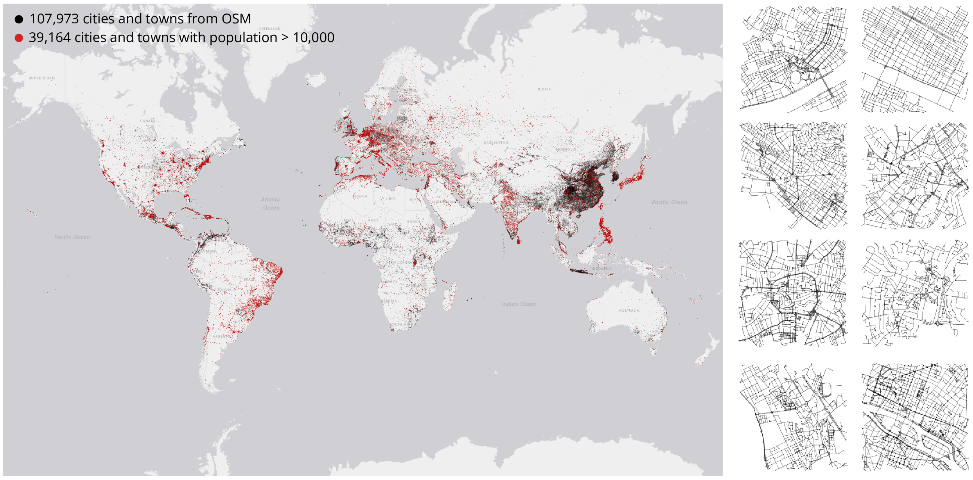
The street network dataset is from OpenStreetMap (OSM) [8], a publicly available geographic database of the world. Street networks are represented as piecewise-linear polylines with an associated highway label to distinguish them from other geographical structures. The raw road network extracted from OSM is represented as a vector containing its geographic coordinates in the WGS84 projection. We query all cities and towns, totaling 107,973, by extracting all features that have a place tag equal to town or city. These centers do not necessarily correspond to defined cities but are important urban centers with many shops and facilities. We also extract any information related to the population for these centers to subset the initial data for different tasks. As per OSM, 34% of nodes tagged as towns have a population tag, and the median value in the database varies by country, from as low as 300 to as high as 35,000. 95% of towns have a population=* value between 1000 and 70,000. In the case of nodes tagged as cities, 63% have a population tag, of which the median value is 130,000, and 95% of them have a population value over 20,000. To train the model, we use a subset of cities containing a population tag valued over 1000. This results in a total of 39,364 cities and towns; the spatial distribution of these cities and towns is shown in Figure 1. Of these networks, the mean number of nodes within the 1 sq km is 430, and the mean number of edges is 1100.

The distribution of the number of nodes and edges in the entire dataset is shown in Figure 2.

For each of the selected cities and towns, we download the street network within a 1 km × 1 km box at the centroid of each place using osmnx [26]. For each grid, we retrieve a graph G = (V, E) where each node v corresponds to a street intersection, and an edge e corresponds to a street segment. Each street network is first re-projected from the given spherical coordinates to meters using the UTM projection for the given area. Then, the street networks are further simplified by joining nodes closer to a threshold of 10 m.

Table 1. Notation summary for the street-network embedding models.

Symbol	Description
$G=(V,E)$	undirected street-network graph
V	set of nodes (street junctions)
E	set of edges (street segments)
C	node feature matrix (coordinates of each node)
A	adjacency matrix of G
$f:G\to {\mathbb{R}}^d$	embedding function mapping G to ${\mathbb{R}}^d$
$p\left(G\right)$	joint distribution over graphs
$p(A,C)$	joint distribution of adjacency and node features
$p(A\mid C)$	conditional distribution of A given C
$p\left(C\right)$	marginal distribution over node features
$C^{\mathrm{seq}}$	flattened ordered sequence of coordinate tokens
$X\in {\mathbb{R}}^{n\times 128}$	learned node-feature embeddings from transformer
$\mathbf{A}$$\in {\{0,1\}}^{n\times n}$	binary adjacency matrix (with 1 on the diagonal)
$\mathbf{D}=\mathrm{diag}\left({\sum }_j{A}_{1j},\dots ,{\sum }_j{A}_{nj}\right)$	degree matrix of A
$\tilde{\mathbf{A}}={\mathbf{D}}^{-1/2}\mathbf{A}{\mathbf{D}}^{-1/2}$	symmetrically normalized adjacency matrix
$\mathbf{Z}\in {\mathbb{R}}^{n\times f}$	matrix of latent variables (${\mathbf{z}}_i$ per node)
$q(\mathbf{Z}\mid \mathbf{X},\mathbf{A})={\prod }_i\mathcal{N}({\mathbf{z}}_i\mid {\mu }_i,\mathrm{diag}\left({\sigma }_i^2\right))$	variational posterior
${\mu }_i,{\sigma }_i^2$	mean and variance of $q({\mathbf{z}}_i\mid \mathbf{X},\mathbf{A})$
$\mathcal{N}(·\mid \mu ,\Sigma )$	multivariate Gaussian distribution
$\mathrm{GCN}(\mathbf{A},\mathbf{X})$	two-layer graph convolutional network
${\mathbf{W}}_0,{\mathbf{W}}_1$	learnable weight matrices of GCN layers
$\mathrm{ReLU}(·)$	rectified linear activation function
$A^{\prime }$	reconstructed adjacency matrix
$p\left(A_{ij}^{\prime }=1\mid {\mathbf{z}}_i,{\mathbf{z}}_j\right)=\sigma \left({\mathbf{z}}_i^{\top }{\mathbf{z}}_j\right)$	decoder edge-existence probability
$\sigma (·)$	logistic sigmoid function
$\mathcal{L}$	variational lower-bound objective
${\mathbb{E}}_{q(\mathbf{Z}\mid \mathbf{A},\mathbf{X})}\left[logp(\mathbf{A}\mid \mathbf{Z})\right]$	expected log-likelihood term
$\mathrm{KL}\left[q(\mathbf{Z}\mid \mathbf{A},\mathbf{X})\parallel p\left(\mathbf{Z}\right)\right]$	Kullback–Leibler divergence term

Table 1. Notation summary for the street-network embedding models.

Symbol	Description
$G=(V,E)$	undirected street-network graph
V	set of nodes (street junctions)
E	set of edges (street segments)
C	node feature matrix (coordinates of each node)
A	adjacency matrix of G
$f:G\to {\mathbb{R}}^d$	embedding function mapping G to ${\mathbb{R}}^d$
$p\left(G\right)$	joint distribution over graphs
$p(A,C)$	joint distribution of adjacency and node features
$p(A\mid C)$	conditional distribution of A given C
$p\left(C\right)$	marginal distribution over node features
$C^{\mathrm{seq}}$	flattened ordered sequence of coordinate tokens
$X\in {\mathbb{R}}^{n\times 128}$	learned node-feature embeddings from transformer
$\mathbf{A}$$\in {\{0,1\}}^{n\times n}$	binary adjacency matrix (with 1 on the diagonal)
$\mathbf{D}=\mathrm{diag}\left({\sum }_j{A}_{1j},\dots ,{\sum }_j{A}_{nj}\right)$	degree matrix of A
$\tilde{\mathbf{A}}={\mathbf{D}}^{-1/2}\mathbf{A}{\mathbf{D}}^{-1/2}$	symmetrically normalized adjacency matrix
$\mathbf{Z}\in {\mathbb{R}}^{n\times f}$	matrix of latent variables (${\mathbf{z}}_i$ per node)
$q(\mathbf{Z}\mid \mathbf{X},\mathbf{A})={\prod }_i\mathcal{N}({\mathbf{z}}_i\mid {\mu }_i,\mathrm{diag}\left({\sigma }_i^2\right))$	variational posterior
${\mu }_i,{\sigma }_i^2$	mean and variance of $q({\mathbf{z}}_i\mid \mathbf{X},\mathbf{A})$
$\mathcal{N}(·\mid \mu ,\Sigma )$	multivariate Gaussian distribution
$\mathrm{GCN}(\mathbf{A},\mathbf{X})$	two-layer graph convolutional network
${\mathbf{W}}_0,{\mathbf{W}}_1$	learnable weight matrices of GCN layers
$\mathrm{ReLU}(·)$	rectified linear activation function
$A^{\prime }$	reconstructed adjacency matrix
$p\left(A_{ij}^{\prime }=1\mid {\mathbf{z}}_i,{\mathbf{z}}_j\right)=\sigma \left({\mathbf{z}}_i^{\top }{\mathbf{z}}_j\right)$	decoder edge-existence probability
$\sigma (·)$	logistic sigmoid function
$\mathcal{L}$	variational lower-bound objective
${\mathbb{E}}_{q(\mathbf{Z}\mid \mathbf{A},\mathbf{X})}\left[logp(\mathbf{A}\mid \mathbf{Z})\right]$	expected log-likelihood term
$\mathrm{KL}\left[q(\mathbf{Z}\mid \mathbf{A},\mathbf{X})\parallel p\left(\mathbf{Z}\right)\right]$	Kullback–Leibler divergence term

3.2. Node Model

The node model aims to estimate a distribution over sequences of nodes. To facilitate this, we impose a node ordering of the lowest to highest by the y coordinate. If nodes have the same y value, we order them by their x coordinate. After imposing a node ordering, we obtain a flattened coordinate sequence $C^{seq}$ by concatenating the coordinate pairs ${(x_i,y_i)}_i$. The coordinate sequence can be decomposed as a joint distribution over its elements as the product of a series of conditional coordinate distributions, as follows:

$$\begin{array}{cc}\hfill p(C^{seq};\theta )& =\prod _{n=1}^{\left|C\right|}p\left(c_n\right|c_{<n};\theta )\hfill \end{array}$$

(2)

We model this distribution using a transformer [27] in an auto-regressive manner, where the prediction of each coordinate depends on all previous coordinates. The model is trained to maximize the log-probability of the observed node distribution with respect to the model parameters $\theta$.

To facilitate learning the spatial distribution of node coordinates, we center each street network at (0, 0) and normalize both x and y coordinates such that the diagonal of their bounding box is equal to 1. Once the nodes are centered and normalized, we apply a uniform 8-bit quantization to model the nodes’ coordinate values as categorical distributions. A similar approach has been taken to model 3D meshes [28] and to discretize continuous signals [29], with the benefit of expressing arbitrary distributions. We find that the spatial extent of 1 km 8-bit quantization does not reduce the overall size of the network, as all nodes fall into different bins.

Similar to PolyGen [28], we use three embeddings that are learned during training for each input token: a coordinate embedding, which indicates where the input token is an x or y coordinate; a positional embedding, which indicates which node in the sequence the token belongs to, and a value embeddings, which expresses a token quantized coordinate value. The output at the final step of the transformer is the logits of the distribution of the quantized coordinate values. We use the embeddings X learned as feature vectors for each node as inputs to the variational graph auto-encoder model.

We note that the imposed fixed ordering based on ascending y and then x coordinates introduces a form of rotational asymmetry: identical graphs under rotation may yield different input sequences and thus different learned distributions. This asymmetry can bias the model toward canonical orientations, thereby reducing rotational invariance. Alternative orderings, such as those induced by space-filling curves (e.g., Hilbert or Z-order curves), can preserve spatial locality while being less sensitive to rotation. However, these alternatives come with increased computational complexity and often introduce non-trivial implementation challenges.

Despite its asymmetry, the fixed $(y,x)$ ordering provides a consistent and deterministic way to linearize node coordinates. This consistency is critical for training stability and comparability across examples. It also aligns with prior work on autoregressive coordinate models [28].

3.3. Graph Auto-Encoder Model

Once we have a series of node embeddings X, we want to estimate the edge distributions by estimating the adjacency matrix for a given set of nodes. To achieve this, we use a variational graph auto-encoder [30], a framework for unsupervised learning on graph-structured data based on the variational auto-encoder [31]. 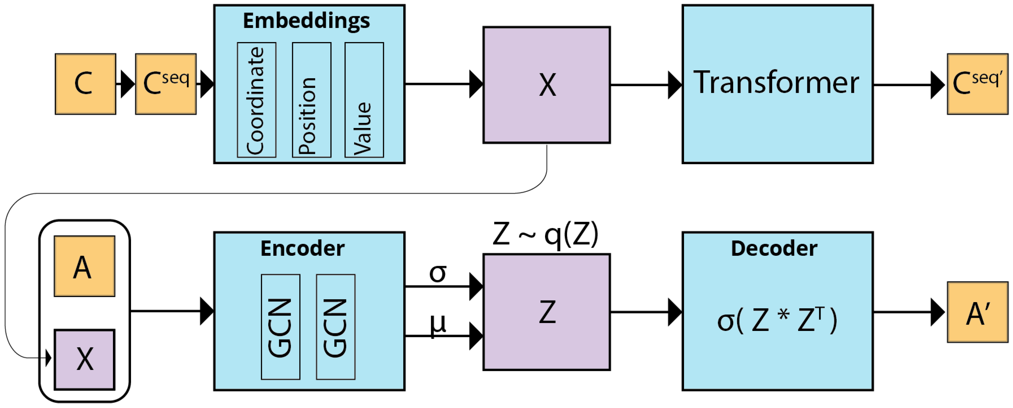The model can learn latent representations for undirected graphs using an adjacency matrix A and the node embeddings X. We use a two-layer convolutional network (GCN) [16] to learn local and global structures present in the data, as shown in Figure 3.

Given the undirected unweighted street network graph G = (V, E) with $n=\left|V\right|$ nodes, we introduce an adjacency matrix $\mathbf{A}\in {0,1}^{n\times n}$ of G with all the diagonal elements equal to one, and its degree matrix $\mathbf{D}=diag\left({\sum }_j{A}_{1j},\dots ,{\sum }_j{A}_{nj}\right)$. We further introduce stochastic latent variables ${\mathbf{z}}_i$, summarized in an $n\times f$ matrix $\mathbf{Z}$, where $f=128$ represents the dimensionality of the latent space for each node in the variational graph auto-encoder. Node features containing the embeddings obtained from the upstream node-embedding model are summarized in an $n\times 128$ matrix $\mathbf{X}$. The variational graph auto-encoder takes in the adjacency matrix $\mathbf{A}$ and the node embeddings $\mathbf{X}$ and learns a new embedding that encodes the topological and node positions.

The encoder of the VGAE is composed of graph convolutional networks (GCNs) and maps $(\mathbf{A},\mathbf{X})$ to a variational posterior over latent variables:

$$q\left(\mathbf{Z}\right|\mathbf{X},\mathbf{A})={\prod }_{i=1}^{N}q\left({\mathbf{z}}_i\right|\mathbf{X},\mathbf{A}),\mathrm{with}q\left({\mathbf{z}}_i\right|\mathbf{X},\mathbf{A})=\mathcal{N}\left({\mathbf{z}}_i\right|{\mu }_i,\mathrm{diag}\left({\sigma }_i^2\right))$$

(3)

The encoder is conditioned on the graph structure $\mathbf{A}$ and node features $\mathbf{X}$ to estimate a multivariate Gaussian distribution for each node’s latent representation ${\mathbf{z}}_i$. Each of these distributions is fully factorized, meaning that the dimensions of ${\mathbf{z}}_i$ are assumed to be independent. The mean ${\mu }_i$ and variance ${\sigma }_i^2$ are learned through GCN layers. Together, these distributions form the variational approximation $q(\mathbf{Z},|,\mathbf{X},\mathbf{A})$ over all node embeddings $\mathbf{Z}$. This setup allows the model to capture uncertainty in the embeddings and enables stochastic training using the reparameterization trick [31].

To compute the parameters of each Gaussian distribution, namely the mean ${\mu }_i$ and log-variance $log{\sigma }_i^2$ for every node i, the encoder employs a shared two-layer GCN. This GCN jointly considers the node features $\mathbf{X}$ and the graph structure captured by $\mathbf{A}$, enabling it to propagate information across the network. The transformation performed by this GCN is defined as

$$\mathrm{GCN}(\mathbf{A},\mathbf{X})=\tilde{\mathbf{A}}\mathrm{ReLU}\left(\tilde{\mathbf{A}}\mathbf{X}{\mathbf{W}}_0\right){\mathbf{W}}_1$$

(4)

where

$$\tilde{\mathbf{A}}={\mathbf{D}}^{-{\displaystyle \frac{1}{2}}}\mathbf{A}{\mathbf{D}}^{-{\displaystyle \frac{1}{2}}}$$

(5)

$\tilde{\mathbf{A}}$ is the symmetrically normalized adjacency matrix, acting as a diffusion operator, smoothing and aggregating feature information over the graph structure. The expression $\tilde{\mathbf{A}}\mathbf{X}{\mathbf{W}}_0$ first applies a linear transformation to the node features using learnable weights ${\mathbf{W}}_0$, followed by graph-based aggregation. This is passed through a ReLU activation to introduce nonlinearity, encouraging sparsity and improving representational capacity. The second layer, $\tilde{\mathbf{A}}(·){\mathbf{W}}_1$, performs another round of aggregation and transformation using weights ${\mathbf{W}}_1$, producing the final latent representations used to parameterize the variational distributions. The same first layer ${\mathbf{W}}_0$ is shared between the networks computing $\mu$ and $log\sigma$ to enforce a common feature basis, while ${\mathbf{W}}_1$ may differ to allow distinct output mappings.

The decoder is defined by a generative model that involves an inner product between latent variables. The output of the decoder is a reconstructed adjacency matrix $A^{\prime }$, which is defined as

$$p\left({\mathbf{A}}^{\prime }|\mathbf{Z}\right)={\prod }_{i=1}^N{\prod }_{j=1}^{N}p\left(A_{ij}^{\prime }|{\mathbf{z}}_i,{\mathbf{z}}_j\right),\mathrm{with}p\left(A_{ij}^{\prime }=1|{\mathbf{z}}_i,{\mathbf{z}}_j\right)=\sigma \left({\mathbf{z}}_i^{\top }{\mathbf{z}}_j\right),$$

(6)

where $A_{ij}^{\prime }$ are the elements of ${\mathbf{A}}^{\prime }$ and $\sigma (·)$ is the logistic sigmoid function.

3.4. Training Objectives

We train the node-sequence transformer and the variational graph auto-encoder in two stages. Each is optimizing a distinct likelihood objective. The node model is trained to maximize the likelihood of a sequence of quantized coordinate tokens $C^{\mathrm{seq}}$. Given transformer parameters $\theta$, we define the negative log-likelihood loss as the categorical cross-entropy:

$${\mathcal{L}}_{\mathrm{node}}\left(\theta \right)=-\sum _{n=1}^{|C^{\mathrm{seq}}|}log{p}_{\theta }(c_n\mid c_{<n}),$$

(7)

where $c_n$ is the n-th token in the sequence and $p_{\theta }(c_n\mid c_{<n})$ is the predicted categorical distribution over 256 quantized coordinate bins for each dimension.

Once node embeddings $\mathbf{X}$ are obtained from the trained transformer, the graph decoder is optimized using the variational evidence lower bound (ELBO) [31]:

$${\mathcal{L}}_{\mathrm{graph}}(\varphi ,\psi )=-{\mathbb{E}}_{q_{\varphi }(\mathbf{Z}\mid \mathbf{A},\mathbf{X})}\left[log{p}_{\psi }(\mathbf{A}\mid \mathbf{Z})\right]+\mathrm{KL}\left[q_{\varphi }(\mathbf{Z}\mid \mathbf{A},\mathbf{X})\parallel p\left(\mathbf{Z}\right)\right],$$

(8)

where $\varphi$ and $\psi$ denote the encoder and decoder parameters, respectively. The likelihood term corresponds to the binary cross-entropy between observed edges in $\mathbf{A}$ and predicted probabilities $\sigma \left({\mathbf{z}}_i^{\top }{\mathbf{z}}_j\right)$. In contrast, the KL term regularizes the posterior $q(\mathbf{Z}\mid \mathbf{A},\mathbf{X})$ towards a standard Gaussian prior $p\left(\mathbf{Z}\right)={\prod }_i\mathcal{N}({\mathbf{z}}_i\mid 0,\mathbf{I})$.

Decoupling node placement from edge generation lets us first sample plausible junction layouts and assess them quickly before incurring the heavier computational cost of synthesizing full connectivity.

The node and variational auto-encoder models were implemented using PyTorch 1.12.0 with the PyTorch Geometric library for graph convolutional layers [32]. Both networks are trained using an 80–20 training–testing split of the entire dataset. The final embeddings we obtain for downstream tasks are created by concatenating embeddings from $\mathbf{Z}$ and further reducing the size of the resulting latent variables by applying a dimensionality reduction that maximizes the variance across the entire training dataset.

4. Results

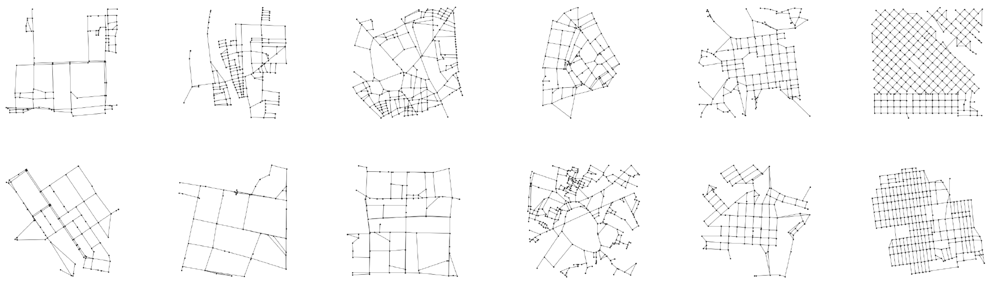
We test the performance of our model by evaluating its capabilities to generate synthetic street networks. We empirically evaluate the quality of network reconstruction by sampling from the learned lower-dimensional latent space and recreating synthetic street networks. The recreated street networks are compared against the street networks in our testing dataset, containing 20% of the data. A sample of synthetic street networks generated from the model is shown in Figure 4. Our model performs well in generating synthetic street networks and accurately captures both the topological and geometric properties of real street networks. However, in some cases, the synthetic data contains some artifacts, such as small triangulated intersections and a series of degree 2 nodes forming one continuous street, we hypothesize that this may be due to the size of the lower dimensional latent space and training time, and further work is needed to test improvements to the model.

4.1. Topological Features

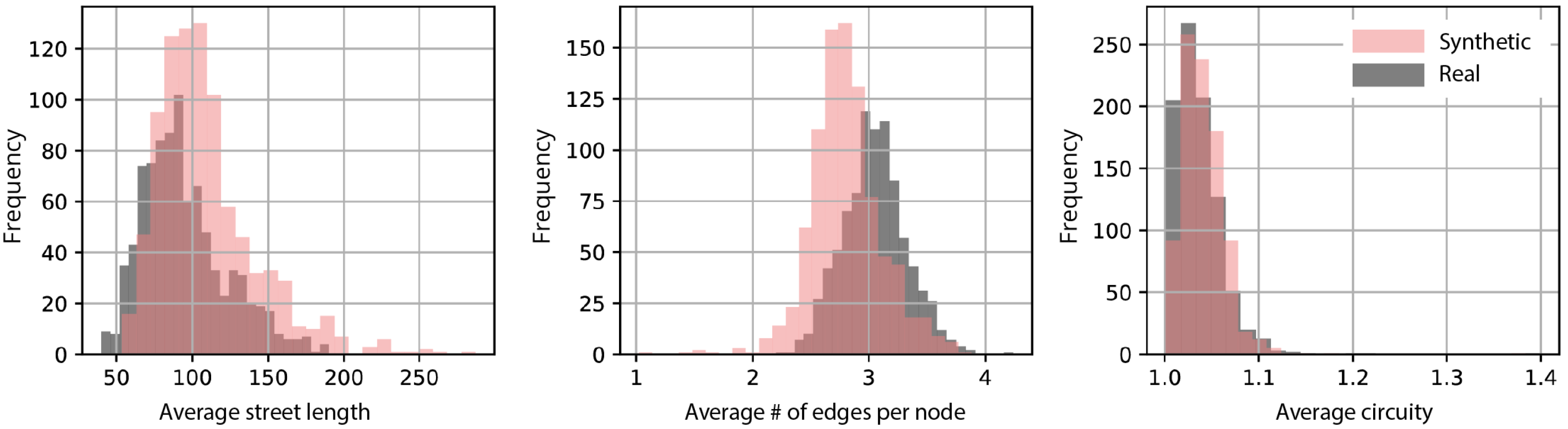
We compare the distribution of certain graph summaries from samples from our model to those of real street networks. If our model closely matches the true data distribution, we expect these summaries to have similar distributions. We draw 1000 samples from our model and 1000 from our testing set. Figure 5 shows kernel density estimates of three key statistics: the average street length, the average number of edges per node, and the average circuity (network distance divided by the Euclidean distance between two neighboring nodes).

These features capture coarse but meaningful structural aspects of urban form. The model captures the overall shape of these distributions with reasonable fidelity, particularly for circuity. However, systematic deviations are evident. The synthetic networks have a higher mean street length ($107.8$ m) compared to real ones ($93.6$ m), with greater variance ($1017.7{\mathrm{m}}^2$ vs. $792.0{\mathrm{m}}^2$). This suggests that the model generates more elongated street segments on average, possibly due to over smoothing in the decoder or insufficient local constraints during generation. Real networks average around 3.05 streets per node, while synthetic ones average 2.81. The variance is also slightly higher in the synthetic set (0.097 vs. 0.082), indicating not only fewer connections but also more variability in intersection complexity. This aligns with our observation that the model tends to overproduce degree-two nodes, possibly as a side effect of sequential generation favoring linear continuation over branching. Lastly, the model captures circuity well, with closely matching means (1.039 synthetic vs. 1.033 real) and similar variance (0.00044 vs. 0.00050). This suggests that at a global level, the generated networks reproduce the overall path complexity of real-world layouts.

To provide a complementary qualitative analysis Figure 6 shows a visual side-by-side comparisons of real and synthetic networks. These samples are matched by different topological properties and illustrate key characteristics such as grid-like patterns, cul-de-sacs, or radial geometries. Visual inspection suggests that the model is able to capture both high-level regularities and localized structural variance in the data, and can produce both regular and organic street patterns.

4.2. Geometric Features

We also compared the distribution of the geometric properties of the generated street networks. For this task, we examine the faces of the planar graph formed by the street, which can be considered city blocks. For each of the graphs representing the testing data and the generated synthetic street networks, we extract the faces of the graph and calculate simple measures to characterize their geometry, allowing us to compare their distributions. We calculate three measures for all the blocks formed by the street network: average block area in square meters, average form factor the ratio between the area of the block and the area of its circumscribed circle, and the average compactness, measured as the ratio of each block’s perimeter length and area. Results are shown in Figure 7. The distribution of the synthetic data’s geometric properties closely matches the real networks.

4.3. Empirical Study of the Learned Embedding—Street Network Classification

4.3.1. Clustering

Following [12], we performed a distance and clustering analysis over the latent representations of each road network, under the premise that the latent space encompasses the main characteristics of the topological structure of the street network. Let $X\left(M\right)=m$ and $X\left(N\right)=n$, $m=(m_1,m_2,\dots ,m_n)$ and $n=(n_1,n_2,\dots ,n_n)$ two vectors in the latent space generated by street network M and street network N, respectively. First, we measured the Euclidean distance $d(m,n)$. If $d(m,n)\to 0$, we conclude that the networks that generated m and n share the same topological characteristics, therefore, in a classification procedure, they should belong to the same cluster. We cluster the obtained $d(m,n)$ values for all studied networks using a K-means approach, with an optimal $K=7$, as determined by the elbow method. So, the clustering is not performed over the actual topological features (where the K-means method would likely perform poorly), but over the set formed by all $d(m,n)$, which is a simple real number vector of size n.

Figure 8 shows the distribution of the cluster membership among all the street networks sections studied. A quarter of the networks belong to cluster number 4, while only 2% belong to cluster number 6. This distribution provides evidence to support the hypothesis that, regardless of their historical differences, street networks can be classified according to their topology and, ultimately, their topological functions [33,34,35,36]. These previous cities’ classification studies are not directly comparable with the classification presented here, because on those, the analysis was conducted over the entire city (not over the smaller street segments), or based on PCA analysis over different city and street indicators, such as a total of resident population and average node degree.

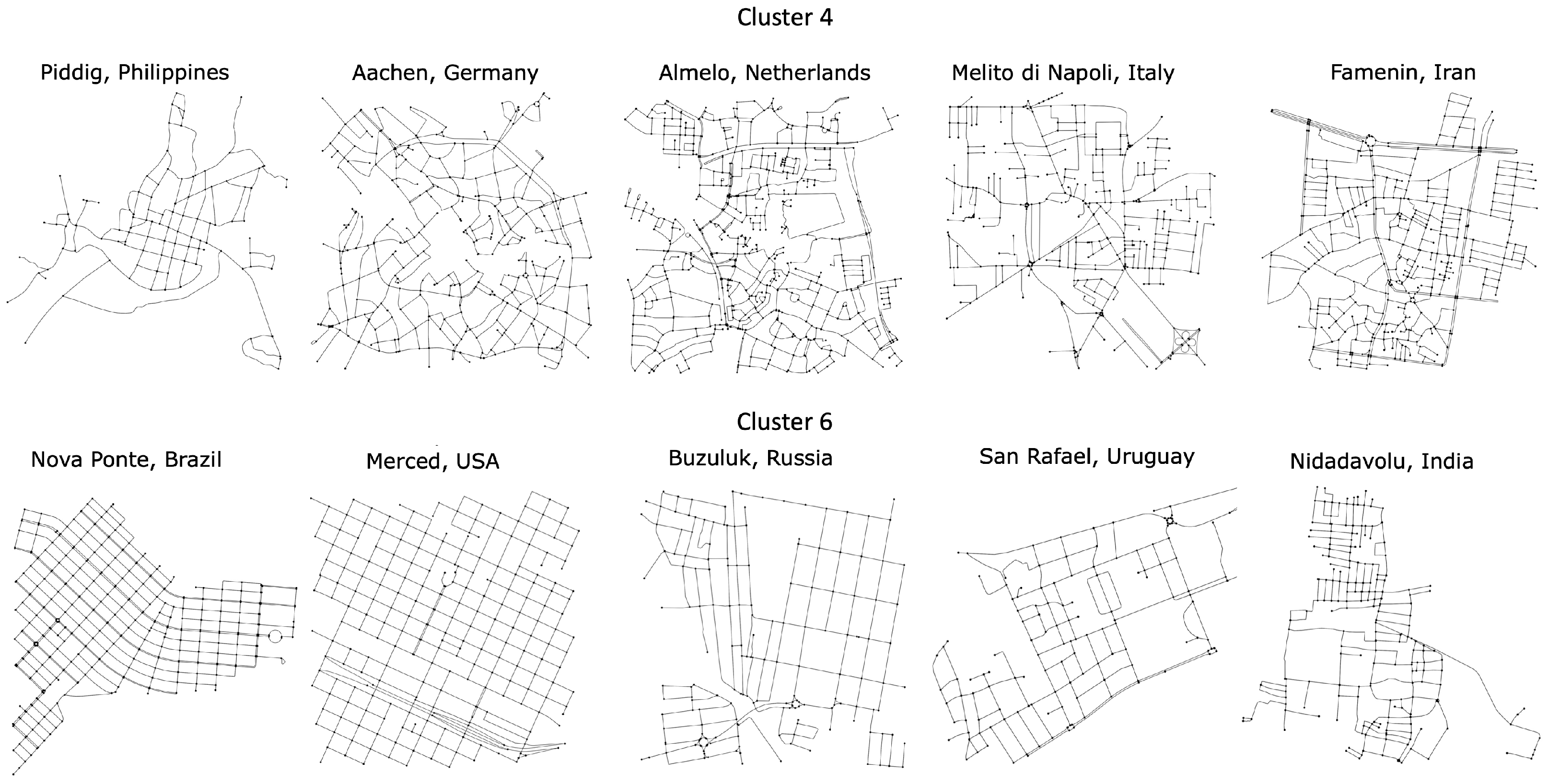
A sample of cluster types 4 and 6 is shown in Figure 9, where some of the topological similarities discussed are visible.

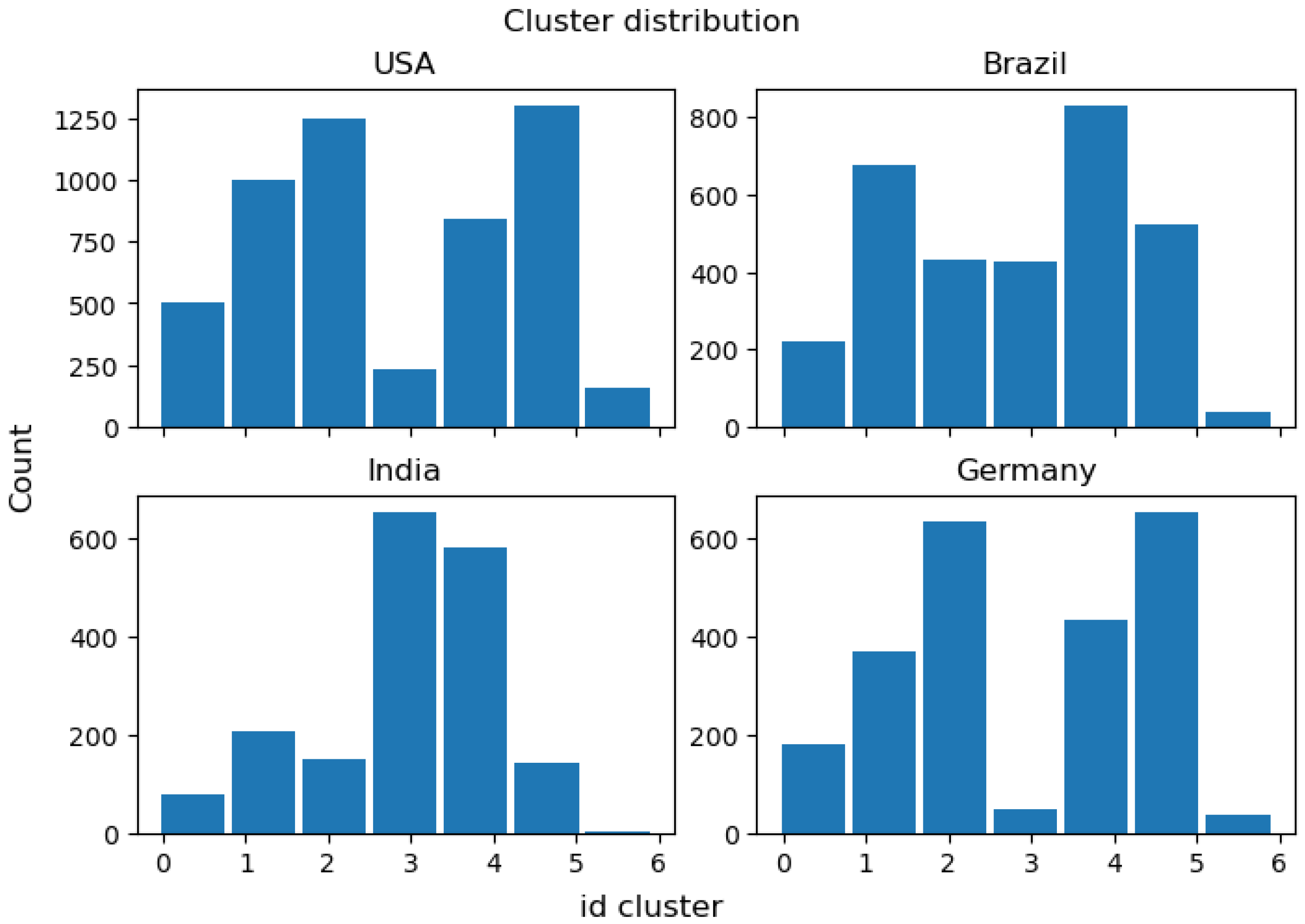
Moving the analysis to individual countries, we observed that the various clusters within each country reveal distinct stories. Inside a country, we can find a wide array of different types of clusters. Most countries have six or seven types of clusters, which show the specific functions and genesis of different segments of the street network within a single city (Figure 10). We also found a significant number of countries with only one type of cluster, with an evident bias towards places with only one street network in the data, which prevents us from deriving a significant conclusion for this cluster of countries.

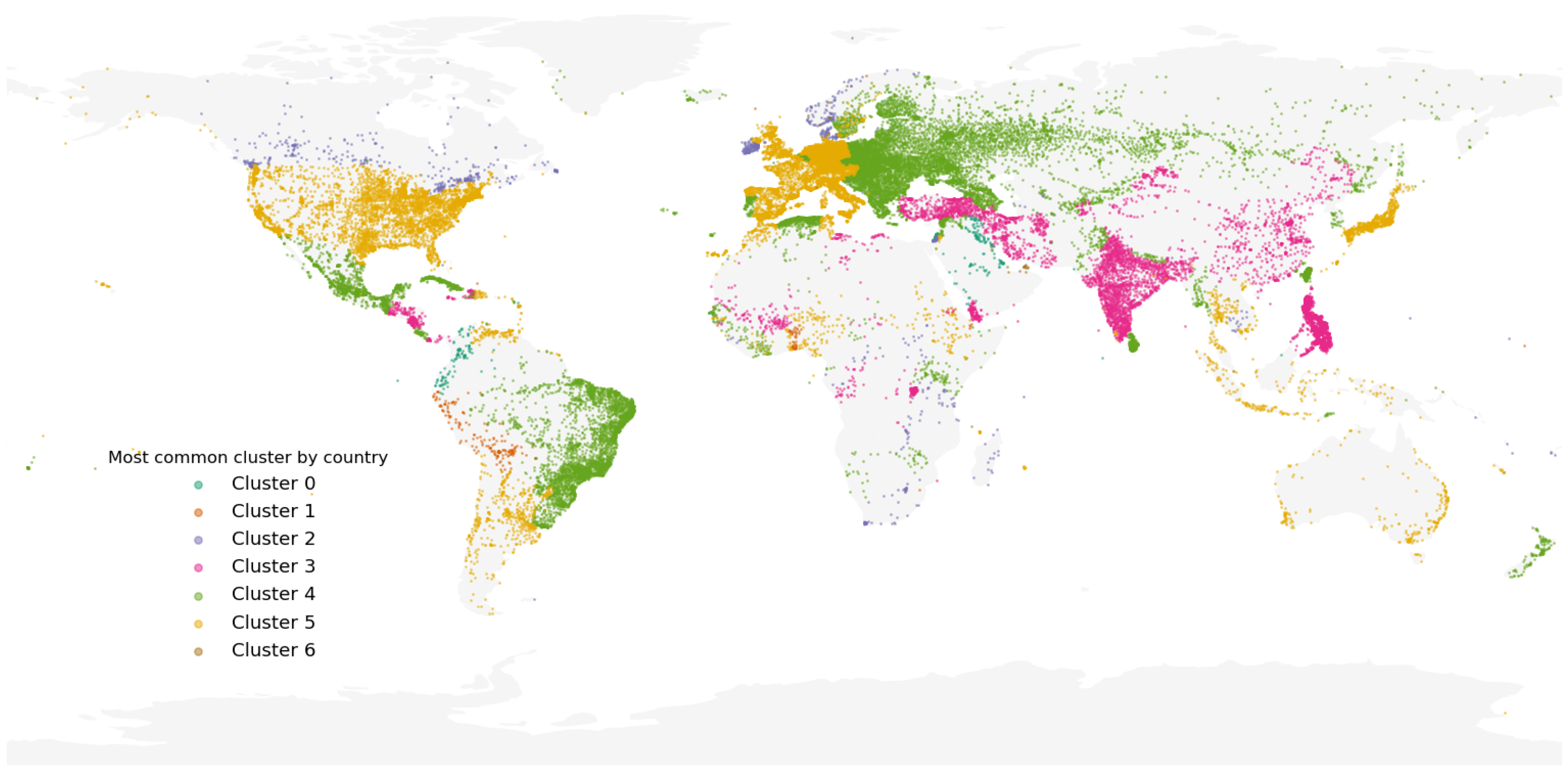
Interestingly, for the 200 states and territories (as defined by OSM’s tag admin_level = 2) included in our study, there is a clear tendency to have a “preferred” cluster, i.e., each cluster membership distribution has a unique mode value. As stated, the main point of this work is not the cluster analysis but the methodology for constructing a latent representation of street networks; however, Figure 11 (which shows the most common membership by country) yields several results that indicate striking similarities between networks across countries. For example, Portugal, Brazil and Mexico share the same local street network structure with some parts of Eastern Europe and Russia. Additionally, we discovered that cluster 3 is the preferred cluster for China, the Philippines, India, Türkiye, and, surprisingly, Central America. The fact that we can observe the same common cluster between Europe and USA presents an interesting research venue that warrants further investigation elsewhere. Finally, we observed that the segments of street networks located in the geographical centers of large cities (e.g., Los Angeles, Mexico City, Mumbai, Cairo, São Paulo, Shanghai) form the less common cluster, cluster number 6.

Nevertheless, the fact that the optimal number of clusters reported (seven) coincides with the one reported in [36] hints about a possible relationship between the latent space and different network properties.

4.3.2. City’s Street Orientation by Cluster Membership

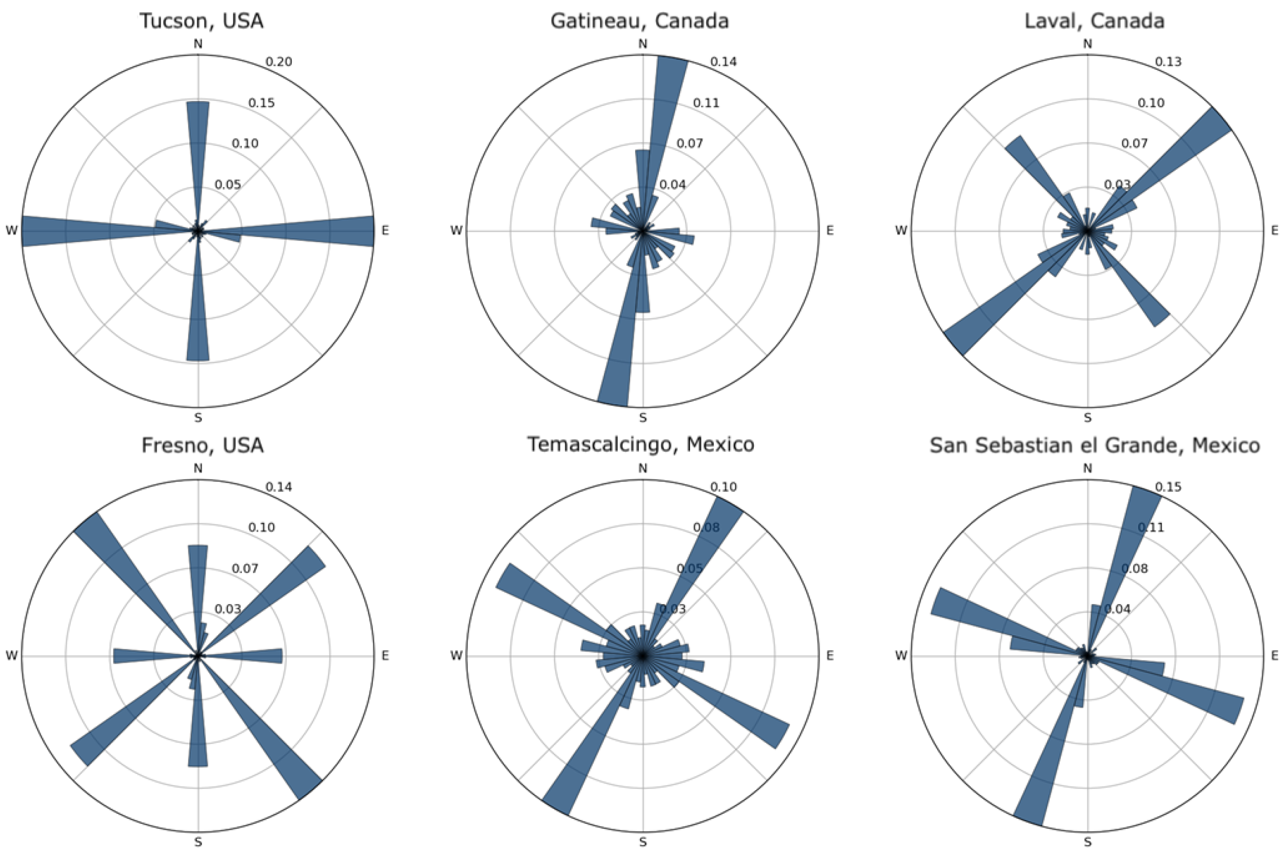
To further evaluate the relevance of our clusters, we look into the street orientation order, following [37]. Our results are not comparable with [37] because the analysis was conducted over the entire city, not over smaller street segments, as in our case. Nevertheless, we found that cities from the same cluster tend to be oriented in the same cardinal direction. For example, the cluster membership mode in Canada is 2, and 90% of all cluster 2 street networks in Canada have a North–East–South–West orientation, like the example in Figure 12. On the other hand, American cities belonging to cluster 5 have an orthogonal orientation, while two small Mexican networks have a strong North–East orientation. As before, these findings need further validation, which is beyond the scope of this paper.

5. Discussion

In this paper, we introduced a two-stage generative framework for street networks that couples an autoregressive node-sequence transformer with a variational graph auto-encoder. The model can infer good latent representations that encode local network structure and the spatial distribution of street intersections. This research contrasts with previous work, which focused on learning representations using computer vision approaches that utilized convolutional layers and relied on creating the raster representations of the street networks before training. Instead, using graph convolutions, we can learn the low-dimensional embedding of street networks directly from their adjacency matrix and a feature matrix encoding the spatial distribution of their nodes.

The model learns directly from street network graphs, using the graph adjacency matrix and a node attribute matrix as inputs, thereby retaining crucial topological information that is often lost when using computer vision models. As a result, the proposed model can generate coherent and diverse street network samples, and the latent representations can be used in downstream tasks such as street network classification. Empirically, the model reproduces key street-network statistics such as average degree, circuity, and block form factor—while generating visually plausible layouts.

Our goal is not to optimize performance on specific downstream benchmarks, but to show that working directly on graph representations enables the model to capture the key structural and spatial properties of street networks in a coherent and interpretable way. By learning from the native graph domain, the model produces embeddings and samples that reflect the geometric and topological diversity of real-world street networks, qualities that are challenging to achieve through image-based approaches.

Despite the positive results, further exploration is necessary. For example, further research is needed to better interpret the learned latent features and their relationship to the topological and geometric properties of the graphs they encode. In particular, structural artifacts observed in some generated networks, such as small triangular intersections and extended sequences of degree-2 nodes, suggest that the model may not fully capture certain street network constraints. These anomalies could stem from factors such as latent space dimensionality or the absence of structural regularization. While incorporating explicit geometric or topological priors offers a promising direction for improvement, strong global constraints such as distance-based regularization risk over-constraining the diversity of historically evolved street patterns. While we do not address these directly in the current work, future research could incorporate targeted regularization strategies or architectural constraints to mitigate such issues, such as hierarchical architectures or geometry-aware edge decoders. Additionally, the model is currently limited to small graphs that only represent a particular place in a city rather than the city as a whole. Since the model requires all graphs to be fixed, entire cities cannot be compared, and the heterogeneity in urban areas is lost.

Street networks operate across nested (hierarchical) scales, from alleyways to arterials to citywide grids. Future work should explore hierarchical models that can progressively grow graphs, possibly via graph diffusion or nested variational approaches. Another limitation stems from the imposed node ordering used in the transformer, which introduces rotational asymmetry. This may introduce systematic biases in the learning process. Incorporating equivariant attention mechanisms or learning a canonical ordering could mitigate these effects.

An immediate implication of the study is that, by learning a useful and compact representation from street networks, we can immediately use this information for other downstream geographical tasks, such as prediction or classification. Additionally, by learning a lower-dimensional embedding and the ability to sample from this latent space and generate a synthetic street network, the model can help shed light on the geometric and topological properties of street networks. This framework also complements traditional urban studies by enabling structured experimentation. For example, it enables interpolating between city forms, exploring how topological properties emerge, or generating counterfactuals that isolate specific network traits, complementing the existing morphological analysis.