Article

Local–Linear Two-Stage Estimation of Local Autoregressive Geographically and Temporally Weighted Regression Model

Department of Mathematics, School of Sciences, Inner Mongolia University of Technology, Hohhot 010051, China
*
Author to whom correspondence should be addressed.
ISPRS Int. J. Geo-Inf. 2025, 14(7), 276; https://doi.org/10.3390/ijgi14070276
Submission received: 1 June 2025 / Revised: 29 June 2025 / Accepted: 14 July 2025 / Published: 16 July 2025

Abstract

A geographically and temporally weighted regression (GTWR) model is an effective tool for dealing with spatial heterogeneity and temporal non-stationarity simultaneously. As an important characteristic of spatiotemporal data, spatiotemporal autocorrelation should be considered when constructing spatiotemporally varying coefficient models. The proposed local autoregressive geographically and temporally weighted regression (GTWRLAR) model can simultaneously handle spatiotemporal autocorrelations among response variables and the spatiotemporal heterogeneity of regression relationships. The two-stage weighted least squares (2SLS) estimation can effectively reduce computational complexity. However, the weighted least squares estimation is essentially a Nadaraya–Watson kernel-smoothing approach for nonparametric regression models, and it suffers from a boundary effect. For spatiotemporally varying coefficient models, the three-dimensional spatiotemporal coefficients (longitude, latitude, and time) inherently exhibit larger boundaries than one-dimensional intervals. Therefore, the boundary effect of the 2SLS estimation of GTWRLAR will be more serious. A local–linear geographically and temporally weighted 2SLS (GTWRLAR-L) estimation is proposed to correct the boundary effect in both the spatial and temporal dimensions of GTWRLAR and simultaneously improve parameter estimation accuracy. The simulation experiment shows that the GTWRLAR-L method reduces the root mean square error (RMSE) of parameter estimates compared to the standard GTWRLAR approach. Empirical analyses of carbon emissions in China’s Yellow River Basin (2017–2021) show that GTWRLAR-L enhances the adjusted R 2 from 0.888 to 0.893.

1. Introduction

Spatial data can be discovered in numerous practical domains, including econometrics, geography, and environmental science. As two basic properties inherent to spatial data, spatial heterogeneity and spatial autocorrelation are universally recognized as coexisting [1,2]. In spatial data modeling, when quantitatively analyzing the relationship between a response variable and explanatory variables, these two properties need to be considered simultaneously.
As an effective tool for dealing with the spatial heterogeneity of regression relationships, geographically weighted regression (GWR) model was initially proposed by Brunsdon et al. [3]. A remarkable characteristic of this model is its capacity to enable parameters to change correspondingly according to different geographical locations. In addition, people increasingly acknowledge time as a critical dimension of human activities and natural phenomena [4,5]. Time data can provide valuable dynamic information for potential spatial processes. To enable the GWR model to simultaneously simulate the temporal heterogeneity effect, Huang et al. [4] and Fotheringham et al. [5] proposed geographically and temporally weighted regression (GTWR) models and used the geographically and temporally weighted least squares estimation method to fit the model. Subsequently, the model’s utility has been widely adopted in various fields, including environmental science [6,7], ecological analyses [8,9], transportation sectors [10,11,12], epidemiological studies [13], and urban studies [14].
However, as Pace and LeSage [15] pointed out, when GWR models are used for simulation fitting, although the optimal bandwidth is determined through optimization, the spatial autocorrelation of the response variable may still not be effectively captured by the models. In addition, Geniaux and Martinetti [16] emphasized that ignoring spatial autocorrelation or heterogeneity may lead to biases in the parameter estimation of the model. Therefore, comprehensive models capable of handling both spatial autocorrelation and spatial heterogeneity simultaneously should attract attention. In fact, since GWR was proposed, various improved methods for the model have been developed according to the actual situation. For example, Brunsdon et al. [17] incorporated a spatially autoregressive term of the response variable into GWR and combined the GWR technique with the maximum likelihood approach to enhance model fit. Sun et al. [18] developed a quasi-maximum likelihood profile estimator using local linearization techniques to calibrate GWR models with global spatial lag effects (SARGWR). This method can solve the boundary effect of the GWR model. Geniaux and Martinetti [16] proposed a class of local regression models that can simultaneously handle spatial autocorrelation and heterogeneity. In this class of models, autoregressive coefficients are diverse and can be either global or local. This design makes the models more flexible and can better capture the complex relationships in spatial data. Gao et al. [19] considered the operational scale problem of spatial processes based on the SARGWR model proposed by Sun et al. [18] and proposed a local–linear multiscale geographically weighted two-stage least squares estimation for the SARGWR model. Based on the SARGWR model and its parameter estimation method proposed by Gao et al. [19] and Sun et al. [18], Mei and Chen [20] considered a more general spatial autoregressive varying coefficient model, and they proposed a bootstrap test for identifying spatial heterogeneity in spatial lag terms and regression relationships. Although these regression models, which integrate spatial autocorrelation and spatial heterogeneity, fully capture the spatial characteristics of geographic information data, they lack an explanation of the time effect in the data. In spatiotemporal data modeling, the time effect provides critical dynamic information for spatial processes, as demonstrated in panel data with temporal sequences.
For this reason, Wu et al. [21] proposed local autoregressive geographically and temporally weighted regression (GTWRLAR) models on the basis of the GTWR model [4] combined with spatial autoregressive (SAR) models. The GTWRLAR model can simultaneously handle local spatiotemporal autocorrelation and heterogeneity characteristics in the data. And they proposed a geographically and temporally weighted two-stage least squares (2SLS) method to estimate the model’s parameters. The 2SLS method is pivotal for two reasons: (i) In spatiotemporal models, the lagged response W · Y is endogenous. The 2SLS method uses instrumental variables to address this, ensuring consistent estimates. (ii) Unlike the maximum likelihood method, the 2SLS estimation avoids setting probability distribution hypotheses for the response variable, thus reducing the computational complexity of models. In fact, whether it is the geographically and temporally weighted least squares estimation of GTWR or the geographically and temporally weighted two-stage least squares estimation of GTWRLAR, they are essentially a Nadaraya–Watson kernel-smoothing approach for non-parametric regression models [22]. The approach has a boundary effect, that is, there will be relatively large parameter estimation biases on the boundary. Although the local–linear GWR model proposed by Wang et al. [23] and the multiscale geographically weighted regression model with local–linear fitting developed by Wu et al. [24] have significantly alleviated the boundary bias problem in two-dimensional spatial scenarios, their technical frameworks face fundamental challenges in three-dimensional spatiotemporal modeling. The traditional local–linear method corrects the parameter estimation in the boundary area through the first-order Taylor′ expansion of the spatial coordinates (longitude and latitude). However, the GTWRLAR model needs to simultaneously analyze the three-dimensional gradient interactions of spatiotemporal coordinates (longitude, latitude, and time), which makes the handling of boundary effects more complex.
Therefore, building upon the GTWRLAR framework, this paper implements a joint linear expansion of the spatial and temporal dimensions within the spatiotemporal neighborhood and proposes a local–linear geographically and temporally weighted two-stage least squares estimation method for the GTWRLAR model. The proposed method not only effectively mitigates the boundary effects in both spatial and temporal dimensions of GTWRLAR but also enhances the accuracy of coefficient estimators by reducing bias in edge regions. These improvements are critical, as accurate coefficient estimators play a pivotal role in correctly interpreting the autocorrelation and heterogeneity characteristics of spatiotemporal processes.
The rest of this article is organized as follows: In Section 2, the GTWRLAR model and local–constant 2SLS estimation of the GTWRLAR model are briefly reviewed, on which its local–linear 2SLS estimation is derived. In Section 3, a simulation experiment is constructed to test the effectiveness of the proposed method. Section 4 verifies the practicability of the proposed method through a real-life example. In Section 5, this paper is concluded, and a discussion is provided.

2. Methods

2.1. GTWRLAR Model

The GTWR model is widely used to address spatiotemporal heterogeneity by allowing regression coefficients to vary with spatiotemporal locations (see Huang et al. [4] for details). Building on this framework, the GTWRLAR model was proposed by Wu et al. [21]. However, the model studied in this paper differs from their work. Specifically, our dataset contains spatial panel data with n spatial units ( i = 1 , 2 , , n ), where each unit corresponds to T time observations ( l = 1 , 2 , , T ). Different from the single-observation housing price data used by Wu et al. [21], each spatial unit in the data of this paper has multiple time observations (that is, the same region contains a dynamic sequence of T periods). Therefore, the GTWRLAR model constructed needs to adapt to this temporal panel feature, and its specific form can be expressed as follows:
y i l = ρ ( u i , v i , t l ) j = 1 , j i n w i j l y j l + k = 1 p β k ( u i , v i , t l ) x i l k + ε i l , i = 1 , 2 , , n , l = 1 , 2 , , T ,
where i = 1 , , n denotes spatial units, l = 1 , , T denotes time periods, j indexes neighboring spatial units, and k = 1 , , p indexes explanatory variables. ( u i , v i , t l ) represent the longitude, latitude, and time of the i-th spatial unit at period l. ρ ( u i , v i , t l ) denotes the autoregressive coefficient, which reflects the spatiotemporal autocorrelation intensity in the response variable. y i l and x i l 1 , x i l 2 , , x i l p are the observed values of the response variable and explanatory variables at the spatiotemporal location ( u i , v i , t l ) . β ( u i , v i , t l ) = ( β 1 ( u i , v i , t l ) , β 2 ( u i , v i , t l ) , , β p ( u i , v i , t l ) ) T is an unknown smooth function with respect to ( u i , v i , t l ) . w i j l represents an element of the n order spatial adjacency matrix W l at the l-th time stamp, with the same construction at each time stamp. The independent and identically distributed ε i l represents the errors of the model. Generally, it is assumed that the error terms have a zero mean and the same variance.
To simplify the presentation, let Y = y 11 , , y n 1 , y 12 , , y n 2 , , y 1 T , , y n T T . ρ ( u , v , t ) is a block diagonal matrix of order T × T , where the l-th sub-block is ρ l = Diag ( ρ ( u 1 , v 1 , t l ) , , ρ ( u n , v n , t l ) ) . W is a block diagonal matrix of order T × T , where the l-th sub-block is W l = ( w i j l ) n × n , and M ( u , v , t ) = ( M 1 ( u , v , t ) , , M T ( u , v , t ) ) T , where M l ( u , v , t ) = ( x 1 l T β ( u 1 , v 1 , t l ) , , x n l T β ( u n , v n , t l ) ) . Here, x i l T = ( x i l 1 , , x i l p ) is the i-th row of the n × p matrix X l , l = 1 , 2 , , T , and X n T × p = ( X 1 , , X T ) T . ε = ε 11 , , ε n 1 , ε 12 , , ε n 2 , , ε 1 T , , ε n T T . The GTWRLAR model in Equation (1) using matrix notation can be expressed as follows:
Y = ρ ( u , v , t ) W · Y + M ( u , v , t ) + ε ,

2.2. Local–Constant 2SLS Estimation of the GTWRLAR Model

When estimating the parameters of the model, the endogeneity problem must be addressed first. An instrumental variable is a variable correlated with the endogenous variable but uncorrelated with the error term, and it is used to address endogeneity and obtain consistent parameter estimates. In the above model, W · Y is endogenous (due to its correlation with the error term ε ), so an instrumental estimator of W · Y is needed to obtain consistent estimates using least squares estimation. As suggested by Geniaux and Martinetti [16], as well as by Mei and Chen [20], the instrumental variables Q = ( X , WX , W 2 X ) , where X is the design matrix and its first column is not the constant term, can be used to estimate W · Y by formulating the following GTWR model:
y w i l = j = 1 , j i n w i j l y j l = q i l T γ ( u i , v i , t l ) + η i l , i = 1 , 2 , , n , l = 1 , 2 , , T ,
where q i l T = ( q i 1 l , q i 2 l , , q i , 3 p , l ) is the i-th row of the instrumental variable Q n T × 3 p at the l-th time stamp. Using the Nadaraya–Watson kernel-smoothing-based geographically and temporally weighted least squares estimation [4] to fit the model (3), the fitted value of the spatiotemporal lag term W · Y can be obtained as follows:
y ^ w = ( y ^ w 11 , , y ^ w n 1 , y ^ w 12 , , y ^ w n 2 , , y ^ w 1 T , , y ^ w n T ) T = L Q ( h S , h T ) W · Y ,
where
L Q ( h S , h T ) = q 1 T Q T W S T ( u 1 , v 1 , t 1 ) Q 1 Q T W S T ( u 1 , v 1 , t 1 ) q n T Q T W S T ( u n , v n , t 1 ) Q 1 Q T W S T ( u n , v n , t 1 ) q n + 1 T Q T W S T ( u 1 , v 1 , t 2 ) Q 1 Q T W S T ( u 1 , v 1 , t 2 ) q 2 n T Q T W S T ( u n , v n , t 2 ) Q 1 Q T W S T ( u n , v n , t 2 ) q n ( T 1 ) + 1 T Q T W S T ( u 1 , v 1 , t T ) Q 1 Q T W S T ( u 1 , v 1 , t T ) q n T T Q T W S T ( u n , v n , t T ) Q 1 Q T W S T ( u n , v n , t T ) .
Replacing j = 1 , j i n w i j l y j l in Equation (1) with y ^ w i l in Equation (4), this leads to the reformulation of Equation (1) as
y i l = ρ ( u i , v i , t l ) y ^ w i l + k = 1 p β k ( u i , v i , t l ) x i l k + ε i l = z i l T α ( u i , v i , t l ) + ε i l , i = 1 , 2 , , n , l = 1 , 2 , , T .
Let α ( u i , v i , t l ) = ( ρ ( u i , v i , t l ) , β T ( u i , v i , t l ) ) T and Z = y ^ w , X , the model (6) can be regarded as a GTWR model with the regression coefficients being α ( u i , v i , t l ) . Using geographically and temporally weighted least squares estimation, the estimate of coefficient vector at the spatiotemporal location ( u i , v i , t l ) is
α ^ G ( u i , v i , t l ) = ( ρ ^ ( u i , v i , t l ) , β ^ 1 ( u i , v i , t l ) , , β ^ p ( u i , v i , t l ) ) T = ( Z T W S T ( u i , v i , t l ) Z ) 1 Z T W S T ( u i , v i , t l ) Y .
where the subscript “G” denotes the local–constant estimation method. The estimated response vector is
Y ^ G = ( y ^ G 11 , , y ^ G n 1 , y ^ G 12 , , y ^ G n 2 , , y ^ G 1 T , , y ^ G n T ) T = L G ( h S , h T ) Y ,
where
L G ( h S , h T ) = z 11 T Z T W S T ( u 1 , v 1 , t 1 ) Z 1 Z T W S T ( u 1 , v 1 , t 1 ) z n 1 T Z T W S T ( u n , v n , t 1 ) Z 1 Z T W S T ( u n , v n , t 1 ) z 12 T Z T W S T ( u 1 , v 1 , t 2 ) Z 1 Z T W S T ( u 1 , v 1 , t 2 ) z n 2 T Z T W S T ( u n , v n , t 2 ) Z 1 Z T W S T ( u n , v n , t 2 ) z 1 T T Z T W S T ( u 1 , v 1 , t T ) Z 1 Z T W S T ( u 1 , v 1 , t T ) z n T T Z T W S T ( u n , v n , t T ) Z 1 Z T W S T ( u n , v n , t T )
is a hat matrix. z i l T = y ^ w i l , x i l T is the i-th row of the design matrix Z at the l-th time stamp, i = 1 , 2 , , n , l = 1 , 2 , , T .
The residual vector is
ε ^ G = ( ε ^ G 11 , , ε ^ G n 1 , ε ^ G 12 , , ε ^ G n 2 , , ε ^ G 1 T , , ε ^ G n T ) T = I n L G ( h S , h T ) Y .
The residual sum of squares is
RSS G ( h S , h T ) = ε ^ G T ε ^ G = Y T ( I n L G ( h S , h T ) ) T ( I n L G ( h S , h T ) ) Y ,

2.3. Local–Linear 2SLS Estimation of the GTWRLAR Model

In what follows, we extend the local–constant 2SLS estimation of the GTWRLAR model to local–linear 2SLS estimation.
The model in Equation (6) can be expressed equivalently in the following form:
y i l = z i l T α ( u i , v i , t l ) + ε i l , i = 1 , 2 , , n , l = 1 , 2 , , T ,
Assume that each coefficient function α k u , v , t k = 1 , 2 , , p + 1 in Equation (12) has continuous partial derivatives with respect to the spatiotemporal domain ( u , v , t ) . We use a first-order Taylor’s expansion at any given location ( u 0 , v 0 , t 0 ) in the study area. For each k = 1 , 2 , , p + 1 , this yields a locally linear approximation of α k u , v , t :
α k ( u , v , t ) α k ( u 0 , v 0 , t 0 ) + α k ( u ) ( u 0 , v 0 , t 0 ) ( u u 0 ) + α k ( v ) ( u 0 , v 0 , t 0 ) ( v v 0 ) + α k ( t ) ( u 0 , v 0 , t 0 ) ( t t 0 ) ,
where α k ( u ) ( u 0 , v 0 , t 0 ) , α k ( v ) ( u 0 , v 0 , t 0 ) , and α k ( t ) ( u 0 , v 0 , t 0 ) are the partial derivatives of α k ( u 0 , v 0 , t 0 ) at location ( u 0 , v 0 , t 0 ) with respect to u, v, and t, respectively. By replacing the coefficients α k ( u , v , t ) in Equation (12) with the expression in Equation (13) and constructing a weighted least squares problem, we minimize the following objective function with respect to α k ( u ) ( u 0 , v 0 , t 0 ) , α k ( v ) ( u 0 , v 0 , t 0 ) , and α k ( t ) ( u 0 , v 0 , t 0 )   ( k = 1 , 2 , , p + 1 ) .
i = 1 n l = 1 T ( y i l k = 1 p + 1 ( α k ( u 0 , v 0 , t 0 ) + α k ( u ) ( u 0 , v 0 , t 0 ) ( u i u 0 ) + α k ( v ) ( u 0 , v 0 , t 0 ) ( v i v 0 ) + α k ( t ) ( u 0 , v 0 , t 0 ) ( t l t 0 ) ) z i l k ) 2 w i l S T ( u 0 , v 0 , t 0 ) ,
Let θ ( u 0 , v 0 , t 0 ) = α ( u 0 , v 0 , t 0 ) T , ( α ( u ) ( u 0 , v 0 , t 0 ) ) T , ( α ( v ) ( u 0 , v 0 , t 0 ) ) T , ( α ( t ) ( u 0 , v 0 , t 0 ) ) T T , where
α ( u 0 , v 0 , t 0 ) = α 1 ( u 0 , v 0 , t 0 ) , , α p + 1 ( u 0 , v 0 , t 0 ) T ,
α ( u ) ( u 0 , v 0 , t 0 ) = α 1 u ( u 0 , v 0 , t 0 ) , , α p + 1 u ( u 0 , v 0 , t 0 ) T ,
α ( v ) ( u 0 , v 0 , t 0 ) = α 1 v ( u 0 , v 0 , t 0 ) , , α p + 1 v ( u 0 , v 0 , t 0 ) T ,
α ( t ) ( u 0 , v 0 , t 0 ) = α 1 t ( u 0 , v 0 , t 0 ) , , α p + 1 t ( u 0 , v 0 , t 0 ) T .
Define Z ( u 0 , v 0 , t 0 ) = Z , Z ( u u 0 ) , Z ( v v 0 ) , Z ( t t 0 ) , where
Z ( u u 0 ) = y ^ w 11 ( u 1 u 0 ) x 111 ( u 1 u 0 ) x 11 p ( u 1 u 0 ) y ^ w n 1 ( u n u 0 ) x n 11 ( u n u 0 ) x n 1 p ( u n u 0 ) y ^ w 12 ( u 1 u 0 ) x 121 ( u 1 u 0 ) x 12 p ( u 1 u 0 ) y ^ w n 2 ( u n u 0 ) x n 21 ( u n u 0 ) x n 2 p ( u n u 0 ) y ^ w 1 T ( u 1 u 0 ) x 1 T 1 ( u 1 u 0 ) x 1 T p ( u 1 u 0 ) y ^ w n T ( u n u 0 ) x n T 1 ( u n u 0 ) x n T p ( u n u 0 ) ,
Z ( v v 0 ) = y ^ w 11 ( v 1 v 0 ) x 111 ( v 1 v 0 ) x 11 p ( v 1 v 0 ) y ^ w n 1 ( v n v 0 ) x n 11 ( v n v 0 ) x n 1 p ( v n v 0 ) y ^ w 12 ( v 1 v 0 ) x 121 ( v 1 v 0 ) x 12 p ( v 1 v 0 ) y ^ w n 2 ( v n v 0 ) x n 21 ( v n v 0 ) x n 2 p ( v n v 0 ) y ^ w 1 T ( v 1 v 0 ) x 1 T 1 ( v 1 v 0 ) x 1 T p ( v 1 v 0 ) y ^ w n T ( v n v 0 ) x n T 1 ( v n v 0 ) x n T p ( v n v 0 ) ,
Z ( t t 0 ) = y ^ w 11 ( t 1 t 0 ) x 111 ( t 1 t 0 ) x 11 p ( t 1 t 0 ) y ^ w n 1 ( t T t 0 ) x n 11 ( t T t 0 ) x n 1 p ( t T t 0 ) y ^ w 12 ( t 1 t 0 ) x 121 ( t 1 t 0 ) x 12 p ( t 1 t 0 ) y ^ w n 2 ( t T t 0 ) x n 21 ( t T t 0 ) x n 2 p ( t T t 0 ) y ^ w 1 T ( t 1 t 0 ) x 1 T 1 ( t 1 t 0 ) x 1 T p ( t 1 t 0 ) y ^ w n T ( t T t 0 ) x n T 1 ( t T t 0 ) x n T p ( t T t 0 ) .
The weighted least squares estimator derived from Equation (14) provides the estimate of the parameter vector θ ( u 0 , v 0 , t 0 ) at location ( u 0 , v 0 , t 0 ) , which is
θ ^ L ( u 0 , v 0 , t 0 ) = ( α ^ L ( u 0 , v 0 , t 0 ) ) T , ( α ^ L ( u ) ( u 0 , v 0 , t 0 ) ) T , ( α ^ L ( v ) ( u 0 , v 0 , t 0 ) ) T , ( α ^ L ( t ) ( u 0 , v 0 , t 0 ) ) T T = Z T ( u 0 , v 0 , t 0 ) W S T ( u 0 , v 0 , t 0 ) Z ( u 0 , v 0 , t 0 ) 1 Z T ( u 0 , v 0 , t 0 ) W S T ( u 0 , v 0 , t 0 ) ,
where α ^ L ( u 0 , v 0 , t 0 ) , α ^ L ( u ) ( u 0 , v 0 , t 0 ) , α ^ L ( v ) ( u 0 , v 0 , t 0 ) , and α ^ L ( t ) ( u 0 , v 0 , t 0 ) denote the local–linear estimates of α ( u 0 , v 0 , t 0 ) , α ( u ) ( u 0 , v 0 , t 0 ) , α ( v ) ( u 0 , v 0 , t 0 ) , and α ( t ) ( u 0 , v 0 , t 0 ) , respectively. Then, from Equation (15), we can obtain
α ^ L ( u 0 , v 0 , t 0 ) = ( I p + 1 , 0 p + 1 , 0 p + 1 , 0 p + 1 ) θ ^ L ( u 0 , v 0 , t 0 ) α ^ L ( u ) ( u 0 , v 0 , t 0 ) = ( 0 p + 1 , I p + 1 , 0 p + 1 , 0 p + 1 ) θ ^ L ( u 0 , v 0 , t 0 ) α ^ L ( v ) ( u 0 , v 0 , t 0 ) = ( 0 p + 1 , 0 p + 1 , I p + 1 , 0 p + 1 ) θ ^ L ( u 0 , v 0 , t 0 ) α ^ L ( t ) ( u 0 , v 0 , t 0 ) = ( 0 p + 1 , 0 p + 1 , 0 p + 1 , I p + 1 ) θ ^ L ( u 0 , v 0 , t 0 ) ,
where I p + 1 is a unit matrix of order p + 1 , and 0 p + 1 is the corresponding zero matrix. As mentioned above, ( u 0 , v 0 , t 0 ) = ( u i , v i , t l ) and i = 1 , 2 , , n ; l = 1 , 2 , , T , and the estimates of each α k u , v , t and its partial derivatives at each spatiotemporal location can be obtained.
The estimated response vector at each observation location u i , v i , t l is
Y ^ L = ( y ^ L 11 , , y ^ L n 1 , y ^ L 12 , , y ^ L n 2 , , y ^ L 1 T , , y ^ L n T ) T = L L ( h S , h T ) Y ,
where
L L ( h S , h T ) = z 11 T P Z T ( u 1 , v 1 , t 1 ) W S T ( u 1 , v 1 , t 1 ) Z ( u 1 , v 1 , t 1 ) 1 Z T ( u 1 , v 1 , t 1 ) W S T ( u 1 , v 1 , t 1 ) z n 1 T P Z T ( u n , v n , t 1 ) W S T ( u n , v n , t 1 ) Z ( u n , v n , t 1 ) 1 Z T ( u n , v n , t 1 ) W S T ( u n , v n , t 1 ) z 12 T P Z T ( u 1 , v 1 , t 2 ) W S T ( u 1 , v 1 , t 2 ) Z ( u 1 , v 1 , t 2 ) 1 Z T ( u 1 , v 1 , t 2 ) W S T ( u 1 , v 1 , t 2 ) z n 2 T P Z T ( u n , v n , t 2 ) W S T ( u n , v n , t 2 ) Z ( u n , v n , t 2 ) 1 Z T ( u n , v n , t 2 ) W S T ( u n , v n , t 2 ) z 1 T T P Z T ( u 1 , v 1 , t T ) W S T ( u 1 , v 1 , t T ) Z ( u 1 , v 1 , t T ) 1 Z T ( u 1 , v 1 , t T ) W S T ( u 1 , v 1 , t T ) z n T T P Z T ( u n , v n , t T ) W S T ( u n , v n , t T ) Z ( u n , v n , t T ) 1 Z T ( u n , v n , t T ) W S T ( u n , v n , t T )
is a hat matrix. P = I p + 1 , 0 p + 1 , 0 p + 1 , 0 p + 1 , where the subscript “L” denotes the local–linear estimation method.
The residual vector is
ε ^ L = ( ε ^ L 11 , , ε ^ L n 1 , ε ^ L 12 , , ε ^ L n 2 , , ε ^ L 1 T , , ε ^ L n T ) T = I n L L ( h S , h T ) Y .
The residual sum of squares is
RSS L ( h S , h T ) = ε ^ L T ε ^ L = Y T ( I n L L ( h S , h T ) ) T ( I n L L ( h S , h T ) ) Y .

2.4. Generating the Calibration Weights Matrix W S T ( u i , v i , t l ) and Selecting Optimal Spatial and Temporal Bandwidths

Let W S T ( u 0 , v 0 , t 0 ) = Diag ( W 1 S T ( u 0 , v 0 , t 0 ) , W 2 S T ( u 0 , v 0 , t 0 ) , , W T S T ( u 0 , v 0 , t 0 ) ) , where W l S T ( u 0 , v 0 , t 0 ) = Diag ( w 1 l S T ( u 0 , v 0 , t 0 ) , w 2 l S T ( u 0 , v 0 , t 0 ) , , w n l S T ( u 0 , v 0 , t 0 ) ) , l = 1 , 2 , , T ,   w o m S T = K d o m S h S · K d o m T h T . K ( · ) is a kernel function that is monotonically decreasing with respect to both spatial and temporal distances.
h S and h T denote the spatial and temporal bandwidths, respectively. d o m S = ( u o u m ) 2 + ( v o v m ) 2 , d o m T = | t o t m | , o , m = 1 , 2 , , n T .
Generally, taking ( u 0 , v 0 , t 0 ) as each observation point u i , v i , t l ( i = 1 , 2 , , n ; l = 1 , 2 , , T ) in the study area in turn, the spatiotemporal weight matrix at each spatiotemporal location can be obtained.
When determining the elements in the spatiotemporal weight matrix W S T ( u i , v i , t l ) , the spatial and temporal bandwidths need to be selected. For the spatiotemporal weight matrix involved in the instrumental variable estimation of the spatiotemporal lag term, the local–constant 2SLS estimation of GTWRLAR, and the local–linear 2SLS estimation of GTWRLAR mentioned above, the corrected Akaike Information Criterion ( AIC c ) [25] is used in this paper to select the optimal sizes of h S and h T , which are defined as
AIC c ( h S , h T ) = log RSS ( h S , h T ) n + n + tr ( L ( h S , h T ) ) n 2 tr ( L ( h S , h T ) ) ,
where RSS ( h S , h T ) is the residual sum of the squares of the corresponding model. The optimal sizes of h S and h T are for minimizing the AIC c ( h S , h T ) score in Equation (21).
For ease of the presentation, hereinafter, the local–linear 2SLS estimation of the GTWRLAR model is denoted as GTWRLAR-L, and the local–constant 2SLS estimation of the GTWRLAR model is denoted as GTWRLAR-G.

3. Simulation Experiment

In this section, a simulation experiment is conducted to assess the performance of the GTWRLAR-L method. Additionally, to examine the impact of collinearity between explanatory variables on the estimation accuracy of spatiotemporally varying coefficients, different levels of collinearity among the explanatory variables are also considered. All simulation and real data experiments are performed on a medium-spec laptop (Intel(R) Xeon(R) Gold 5218 CPU @ 2.30 GHz with 96 GB using a 64-bit OS) and utilizing R software (version R 4.4.3).

3.1. Data Generation

We simulated data within a unit square spatial domain [ 0 , 1 ] × [ 0 , 1 ] , with temporal observations uniformly sampled at discrete time stamps l = 1 , 2 , , T , spaced at unit intervals. Given that m = 400 , T = 8 , and the full set of spatiotemporal sampling points consists of n = m T coordinates of the form ( u i , v i , t l ) . The m spatial sampling locations { ( u i , v i ) } i = 1 m are generated by independently drawing pairs of random numbers from the uniform distribution U ( 0 , 1 ) , ensuring that each ( u i , v i ) represents a unique, non-latticed position within the spatial domain [ 0 , 1 ] × [ 0 , 1 ] . The spatial coordinates ( u i , v i ) are generated from the uniform distribution U ( 0 , 1 ) for two critical motivations, balancing realism and methodological rigor. First, this approach mimics real-world spatial sampling by avoiding systematic biases of regular grid layouts, ensuring that points are uniformly spread across the unit square [ 0 , 1 ] × [ 0 , 1 ] . This random sampling offers greater practicality compared to grid-based methods, as it better accommodates irregular spatial configurations in empirical studies. Second, the uniform distribution ensures even sampling near both central and boundary regions, which is critical for evaluating the model’s capability to mitigate boundary effects in edge areas. The temporal index t l = l is restricted to discrete values { 1 , 2 , 3 , 4 , 5 , 6 , 7 , 8 } .
The data generation process is formalized as follows:
y i l = ρ u i , v i , t l j = 1 , j i n w i j l y j l + β 1 u i , v i , t l x i l 1 + β 2 u i , v i , t l x i l 2 + β 3 u i , v i , t l x i l 3 + ε i l ,
where i = 1 , 2 , , n , l = 1 , 2 , , T . The regression coefficients β j ( u , v , t ) ( j = 1 , 2 , 3 ) are designed as follows:
β 1 ( u , v , t ) = ( u + v ) exp t 10 ; β 2 ( u , v , t ) = 32 u v t ( u 1 ) ( v 1 ) ( t 2 ) ; β 3 ( u , v , t ) = 2 1 + cos π v exp t 4 .
The observed values x i l 1 , x i l 2 i = 1 , l = 1 m , T of covariates X 1 and X 2 were randomly and independently drawn from the uniform distribution U ( 2 , 2 ) . The observations of X 3 were generated by
X 3 = γ X 2 + ( 1 γ ) X 30 ,
where 0 γ < 1 , and X 30 denotes independent random variables with the standard normal distribution N ( 0 , 1 ) . It is easy to derive that the correlation coefficient between X 2 and X 3 is
Corr ( X 2 , X 3 ) = Cov ( X 2 , X 3 ) Var ( X 2 ) Var ( X 3 ) = 2 γ 7 γ 2 6 γ + 3 .
In the simulation, four levels of collinearity between X 2 and X 3 were considered:
(i)
γ = 0 , Corr ( X 2 , X 3 ) = 0 .
(ii)
γ = 1 3 , Corr ( X 2 , X 3 ) = 0.5 .
(iii)
γ = 2 3 , Corr ( X 2 , X 3 ) 0.9 .
(iv)
γ = 0.85 , Corr ( X 2 , X 3 ) 0.99 .
Each experimental setting was repeated N times, in which the observations of the explanatory variables were fixed and ε i l i = 1 , l = 1 m , T is generated by the standard normal distribution N ( 0 , 1 ) in each replication.
Design two forms of autoregressive coefficients ρ j u , v , t ( j = 1 , 2 ) , which are, respectively,
ρ 1 ( u , v , t ) = 0.3 + 0.6 ( v 2 u 2 ) t T ; ρ 2 ( u , v , t ) = 0.3 + 0.6 sin π u 2 + v 2 + ( t T ) 2 .
Two forms of autoregressive coefficients have different degrees of spatiotemporal heterogeneity, where the value range of ρ 1 u , v , t is ( 0.3 , 0.9 ) , and the value range of ρ 2 u , v , t is ( 0.9 , 0.3 ) .
In this paper, the l-th time stamp spatiotemporal adjacency matrix W l = w i j l n × n is based on the hexagonal neighbor criterion pointed out by Boots and Tiefelsdorf [26]. Here, the k-nearest neighbor method with k = 6 is selected, and W l at each time stamp has a similar structure. Specifically, we define
w ˜ i j l = 1 , if d i j S h 6 0 , otherwise ,
where h 6 represents the Euclidean distance from the i-th spatiotemporal position ( u i , v i , t l ) to its sixth nearest neighbor. Given i , j = 1 , 2 , , m , if i = j , we set w i j l = 0 ; if i j , we set w i j l = w ˜ i j j = 1 , j i m w ˜ i j l .
The element w i j S T in the spatiotemporal weight matrix W S T ( u i , v i , t l ) is determined by the following bi-square kernel function:
w i j S T = 1 d i j S h k 2 d i j T h T 2 2 , if d i j S h k 2 + d i j T h T 2 1 and t j t i 0 , otherwise ,
where h k is the adaptive spatial bandwidth, representing the Euclidean distance from the point ( u i , v i , t l ) to its k-th nearest neighbor. h T represents the time lag order. k and h T are selected by the AIC c score in Equation (21). Here, h k refers to h S in Equation (21).

3.2. Accuracy Indicators of Simulation Effect

Considering the randomness of data generation, the simulation experiment is repeated N = 200 times. In this paper, common indicators of the root mean square error (RMSE) are selected to evaluate the accuracy of the GTWRLAR-L method and the GTWRLAR-G method in estimating the coefficients of the GTWRLAR model. At the spatiotemporal position ( u i , v i , t l ) , the final estimator of the varying coefficient is the mean of its estimators in N replications. In the GTWRLAR model, let α ^ k ( r ) u i , v i , t l be the estimator of the r-th replication of the k-th varying coefficient at the spatiotemporal position u i , v i , t l . Then, the final estimator of α k u i , v i , t l is
Mean ( α ^ k ( u i , v i , t l ) ) = 1 N r = 1 N α ^ k ( r ) ( u i , v i , t l ) , i = 1 , 2 , , m , l = 1 , 2 , , T ,
The corresponding accuracy indicator, the RMSE, is defined as follows:
RMSE ( α ^ k ( u i , v i , t l ) ) = 1 N r = 1 N ( α ^ k ( r ) ( u i , v i , t l ) α k ( u i , v i , t l ) ) 2 1 2 .
The RMSE measures the difference between estimators and true values. Generally speaking, a lower value of the RMSE indicates higher estimation accuracy.

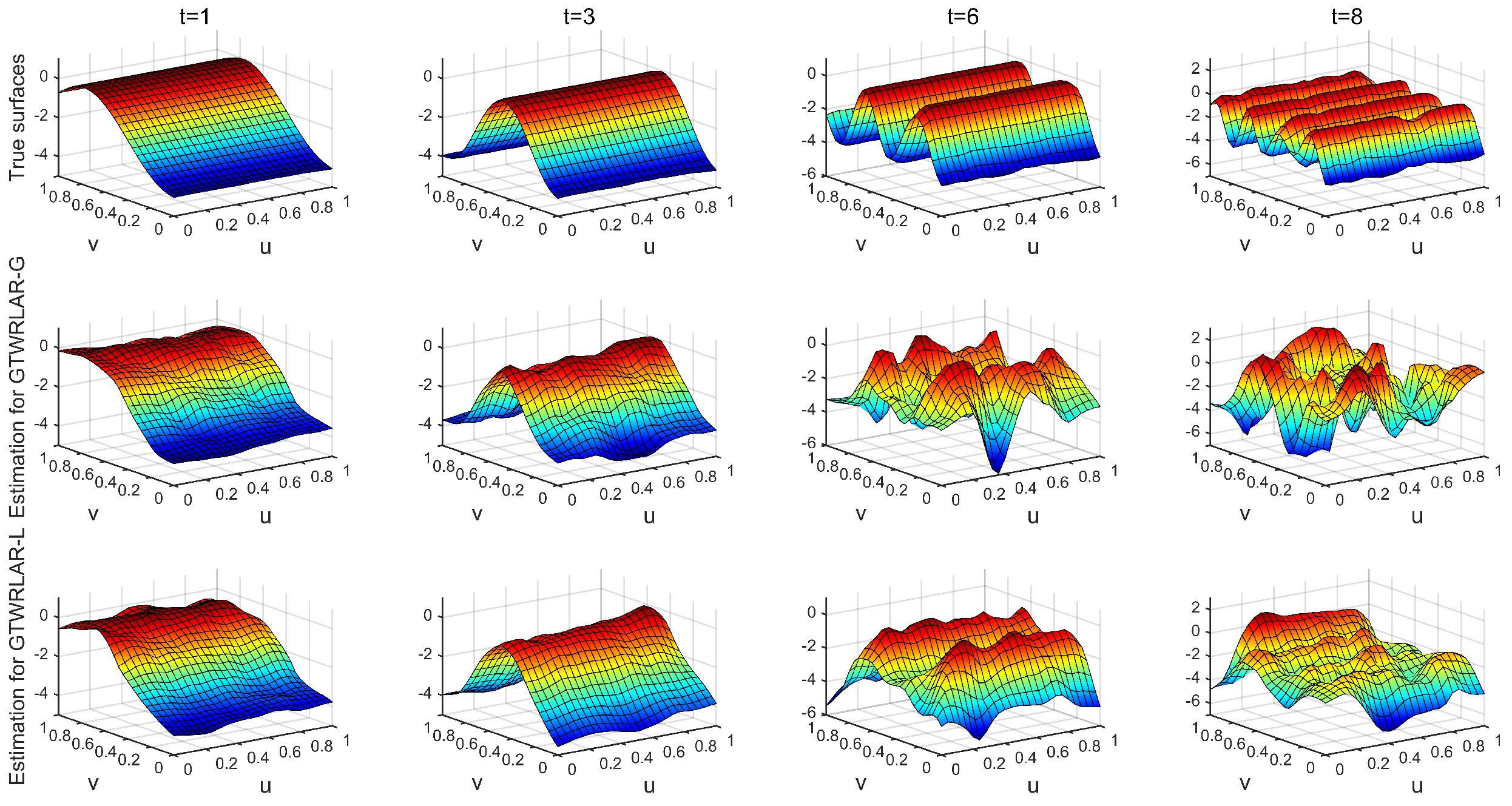
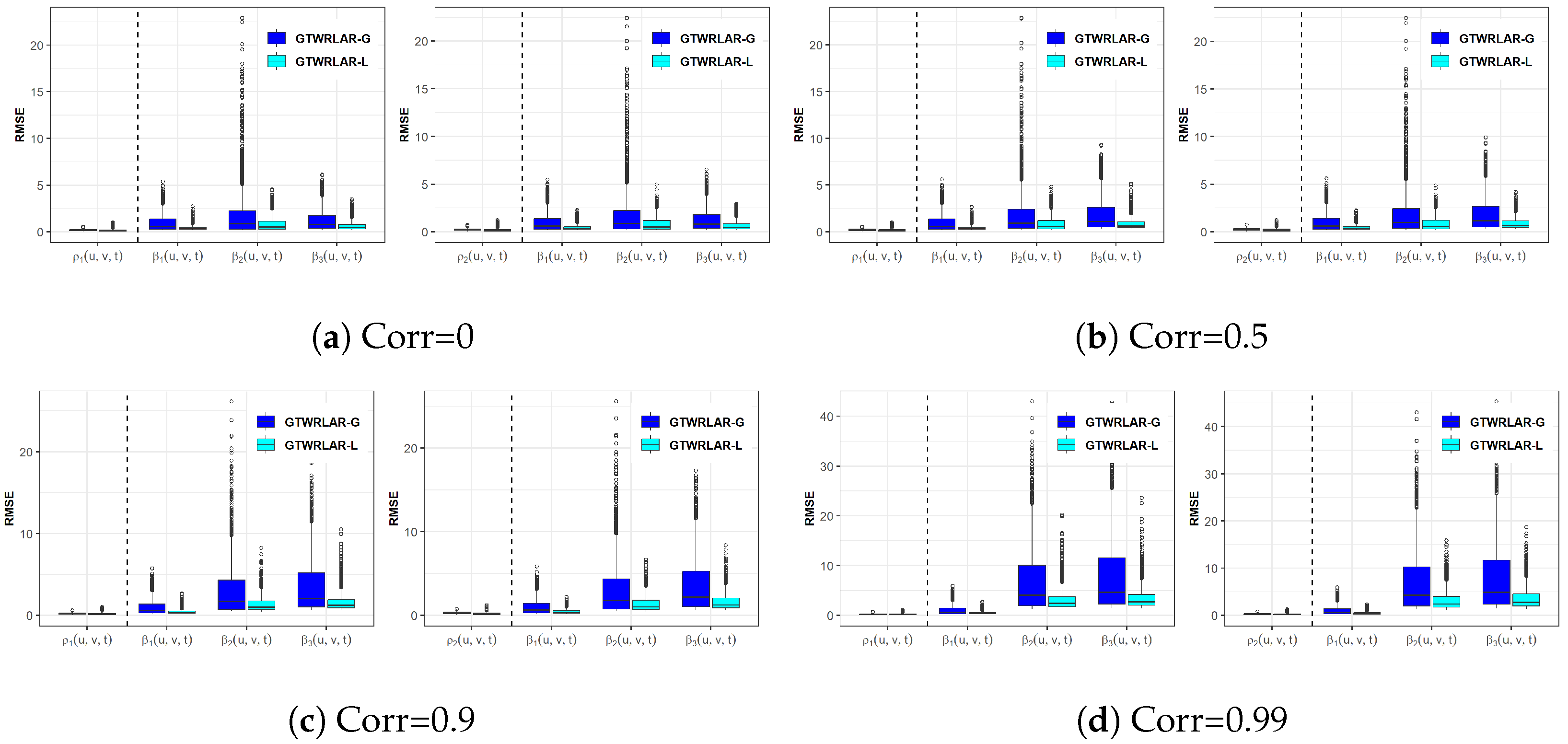
3.3. Simulation Results

Table 1 lists the summary statistics of the optimal spatiotemporal bandwidths, RSS, and AIC c values obtained from 200 replications, and they are obtained using different methods at different correlation levels and under two forms of autoregressive coefficients. It can be observed that irrespective of the degree of spatiotemporal heterogeneity exhibited by the autoregressive coefficients and regardless of whether the explanatory variables in the spatially varying coefficient component are independent or correlated, the GTWRLAR-L framework outperforms the GTWRLAR-G method in terms of both the RSS and AIC c metrics. In addition, when the autoregressive coefficient is ρ 1 ( u , v , t ) , the RSS and AIC c values obtained by GTWRLAR-L are lower than those obtained when the autoregressive coefficient is ρ 2 ( u , v , t ) , but the difference is not significant.
As can be observed in Table 1, the spatiotemporal bandwidths of GTWRLAR-L are sufficiently large and approximately twice those of GTWRLAR-G in the two autoregressive coefficients. Note, however, that the spatiotemporal bandwidths obtained by GTWRLAR-L is the average spatiotemporal bandwidths of α k ( u 0 , v 0 , t 0 ) and its partial derivatives with respect to coordinates u, v, and t at ( u 0 , v 0 , t 0 ) , while the spatiotemporal bandwidths of GTWRLAR-G can be regarded as being obtained only by α k ( u 0 , v 0 , t 0 ) . As mentioned in Wu et al. [24], a direct comparison of absolute bandwidth sizes is inappropriate due to their derivation from different s-order polynomials of the explanatory variable by Taylor’s expansion ( s = 1 or s = 0 ) .
Regarding the impact of collinearity among explanatory variables on the estimation precision of variable coefficients, from Figure 1, it can be seen that for both methods, strong collinearity leads to a decrease in the precision of coefficient estimators. However, the GTWRLAR-L method appears to be less affected. As shown in the figure, when the value of Corr ( X 2 , X 3 ) increases from 0.0 to 0.9, the RMSE values of β 2 ( u , v , t ) and β 3 ( u , v , t ) for the GTWRLAR-G method exhibit a more substantial increase than GTWRLAR-L. These results indicate that the GTWRLAR-L method is more robust to collinearity among explanatory variables than GTWRLAR-G.
To visually compare the coefficient estimator’s accuracy across spatiotemporal locations and time stamps, we depict the true and estimated surfaces of the varying coefficients and autoregressive coefficients ρ 1 ( u , v , t ) and ρ 2 ( u , v , t ) at t = 1, 3, 6, and 8, for different correlation levels, as derived from the GTWRLAR-G and GTWRLAR-L methods. Given the high similarity between the results of the autoregressive coefficients ρ 1 ( u , v , t ) and ρ 2 ( u , v , t ) , we present the surfaces of the regression coefficients only for the case of ρ 1 ( u , v , t ) under the Corr = 0 scenario to save space, as shown in Figure 2, Figure 3 and Figure 4. Figure 5 further presents the true and estimated surfaces of both autoregressive coefficients, other figures are provided in Appendix A. The visualization results reveal that while both methods broadly preserve spatial patterns, and GTWRLAR-L exhibits superior performance in spatial edge regions. The estimated surfaces of GTWRLAR-L maintain the same undulating characteristics as the true surfaces for both regression and autoregressive coefficients. In contrast, GTWRLAR-G exhibits significant spatial boundary distortion.
Meanwhile, GTWRLAR-L significantly outperforms GTWRLAR-G in addressing temporal boundary effects, as evidenced by its stability at time stamps t = 1 (initial) and t = 8 (terminal). By performing first-order Taylor expansion in the temporal neighborhood, GTWRLAR-L captures the instantaneous rate of change, reducing bias in temporal edges. For example, at time stamp t = 3 , the GTWRLAR-G estimated surface of β 2 ( u , v , t ) exhibits significant edge distortion in the temporal domain, whereas GTWRLAR-L retains the true surface’s dynamic trends. Furthermore, the numerical deviation between the estimated surface of GTWRLAR-L and the true surface is smaller, and its coefficient estimators are closer to the true values at all time stamps, demonstrating its robust ability for temporal gradient handling.
The advantages may stem from the spatially and temporally adaptive mechanism of the local polynomial fitting framework: By constructing Taylor expansions within spatial and temporal neighborhoods, the method effectively mitigates systematic biases caused by spatial and temporal truncation effects. Therefore, GTWRLAR-L can mitigate the boundary effects in both spatial and temporal dimensions, whereas the pronounced fluctuations of GTWRLAR-G in edge regions highlight its limitations in handling spatial and temporal boundary interference, failing to achieve the same estimation stability as GTWRLAR-L.

4. A Real-Life Application

4.1. Data Introduction

Following the spatial demarcation of the Yellow River Basin established in prior studies [27,28] and taking the administrative division of the Yellow River Basin in 2020 as the standard, 78 prefecture-level cities were finally identified as the study areas. Referring to the existing literature [29,30,31] and considering data availability, the carbon emission levels (CE (10,000 tons)) of these 78 regions from 2017 to 2021 were used as the dependent variable, with seven explanatory variables were selected. A multicollinearity test was conducted on the processed independent variables. The variance inflation factor (VIF) of each variable is less than 10, indicating that there is no significant collinearity among the variables. All data were compiled from multiple Statistical Yearbooks from 2017 to 2021. The explanatory variables are explained as follows:
  • GDP (CNY): Per capita regional GDP;
  • IIR (%): Proportion of secondary-industry added value in GDP;
  • PP: Permanent population in ten thousand;
  • UR (%): Proportion of urban population;
  • SDE (tons): Industrial sulfur dioxide emissions;
  • DPE (tons): Industrial soot and dust emissions;
  • SWDR (%): Harmless treatment rate of domestic waste.

4.2. Model Construction

To capture the dynamic spatiotemporal interactions between CE and multiple determinants, the above-mentioned GTWRLAR model is adopted. However, before applying the GTWRLAR model to the carbon emission data set, a prerequisite is testing the dataset for spatiotemporal autocorrelation. If no autocorrelation is detected in carbon emissions, the GTWR model suffices for handling spatiotemporal variation. If significant autocorrelation exists in carbon emissions, the GTWRLAR model is preferable. Global Moran’s I is used to test the spatial autocorrelation of carbon emissions in the Yellow River Basin.
The empirical results presented in Table 2 reveal that Moran’s I statistics for CE across 2017–2021 are all positive, with a corresponding Z-value exceeding 2.58 and a p-value falling below 0.001. Additionally, a scatter plot of Moran’s I for all data is shown in Figure 6, demonstrating an overall Moran’s I coefficient of 0.6744 (p < 0.001). These findings confirm the presence of significant spatiotemporal autocorrelation in the dependent variable, thus justifying the adoption of the GTWRLAR model over GTWR to account for autocorrelation effects. Here, we first take the logarithm and then standardize CE and GDP, while other variables are directly standardized. Construct the following GTWRLAR model:
log ( C E i l ) = ρ ( u i , v i , t l ) j = 1 , j i n w i j l log ( CE j l ) + β 1 ( u i , v i , t l ) log ( GDP i l ) + β 2 ( u i , v i , t l ) IIR i l + β 3 ( u i , v i , t l ) PP i l + β 4 ( u i , v i , t l ) UR i l + β 5 ( u i , v i , t l ) SDE i l + β 6 ( u i , v i , t l ) DPE i l + β 7 ( u i , v i , t l ) SWDR i l + ε i l , i = 1 , 2 , , 78 , l = 1 , 2 , , 5 .
The bi-square kernel function is used to generate the spatiotemporal weight matrix. The setting of the spatiotemporal adjacency matrix is the same as that in the simulation experiment. That is, in terms of space, the k-nearest neighbor method with k = 6 is selected. In terms of time, the lag of three time units is selected to define w i j l .

4.3. Result Analysis

For comparative analysis, we applied the same dataset to the traditional GTWR model and the two methods (GTWRLAR-G and GTWRLAR-L) within the GTWRLAR framework. Their diagnostic statistics of R 2 , the residual sum of squares (RSS), and AIC c scores are listed in Table 3. The results show that the R 2 of GTWRLAR-L is 0.893, which is greater than that of GTWRLAR-G (0.888). Notably, the GTWR model exhibits the lowest R 2 (0.871), indicating that when there is spatiotemporal autocorrelation among carbon emissions, using an incorrect model will lead to poor goodness of fit. In addition, the RSS value of GTWRLAR-L (41.495) is lower than that of GTWRLAR-G (43.411) and substantially lower than GTWR’s RSS (50.342). This also validates the conclusion obtained from the simulation experiment: GTWRLAR-L has more advantages in terms of goodness of fit. Existing GTWRLAR models using the GTWRLAR-G method suffer from severe boundary bias due to their kernel-smoothing nature. This bias causes over-smoothing or under-smoothing at dataset edges, distorting spatial pattern interpretation.
Therefore, we use GTWRLAR-L to fit the corresponding spatiotemporally varying coefficients model and analyze the spatiotemporal characteristics of CE and each explanatory variable based on relevant statistical results. The estimated spatiotemporally varying coefficients of the GTWRLAR-L method are summarized in Table 4.
Figure 7 describes the degree of influence of each variable on CE in time and space. As can be seen in Figure 7a, the spatial autoregressive coefficients of carbon emissions in the Yellow River Basin are all positive from 2017 to 2021, indicating positive impacts on a certain region’s carbon emissions from neighboring regions in the current period and from the region itself and neighboring regions in the past. This shows that carbon emission reduction needs cross-regional cooperation and governance [31].
Figure 7b,c show the spatiotemporal variation characteristics of the degree of influence of economic variables (GDP and IIR) on carbon emissions. From 2017 to 2021, the area where GDP has a negative correlation with carbon emissions is relatively large. GDP growth is conducive to increasing investment in clean energy production and energy conservation and emission reduction technologies and reducing carbon emissions [31]. From 2017 to 2021, the spatial characteristics of the impact of IIR on carbon emissions have not changed, mainly showing a positive correlation, and the degree of positive correlation is relatively high in some cities located in the middle and upper Yellow River Basin. The secondary industry has the largest energy demand and consumption and generates the most carbon emissions [32]. Thus, a higher proportion of the secondary industry in the total output value leads to increased carbon emissions.
Figure 7d,e show the spatiotemporal variation characteristics of the degree of influence of population variables (PP and UR) on carbon emissions. From 2017 to 2021, PP and carbon emissions mainly show a positive correlation. Population growth is accompanied by increased consumption demand, which in turn increases energy demand, leading to higher carbon emissions and environmental pressure. The spatiotemporal patterns of UR effects on carbon emissions evolved significantly between 2017 and 2021. While UR exerts a predominantly positive influence from 2017 to 2021 [33], the area of negative correlation gradually expanded in 2021. The reason is that a relatively high urbanization level promotes the agglomeration of factors and economic development [34]. When the economy develops to a certain extent, people have a better environmental protection concept, and total carbon emissions decrease [32].
Figure 7f,h show the spatiotemporal variation characteristics of the degree of influence of ecological variables (SDE, DPE, and SWDR) on carbon emissions. From 2017 to 2021, SDE and carbon emissions mainly show a negative correlation, with the area of negative correlation gradually increasing. In addition, from 2017 to 2019, the area where DPE has a negative correlation with carbon emissions is relatively large, but from 2020 to 2021, it turns into a positive correlation area. During this period, the continuous optimization of industrial and energy consumption structures in many areas led to a transformation of the spatial structure of SDE, DPE, and carbon emissions. From 2017 to 2021, SWDR mainly shows a promoting effect on carbon emissions. Harmless treatment methods may cause chemical reactions to release greenhouse gases and increase total carbon emissions.

5. Conclusions and Future Work

This paper proposes a local–linear geographically and temporally weighted two-stage least squares estimation method for the GTWRLAR model (GTWRLAR-L) to address the inherent limitations of the GTWRLAR model in handling spatial and temporal boundary effects. By integrating local–linear fitting into the 2SLS framework, the proposed method can not only yield the estimators of the coefficients themselves but also derive their partial derivatives with respect to spatial and temporal dimensions. These partial derivatives reveal comprehensive information about dynamic relationships—though this issue is not further explored in this paper. Through simulation experiments comparing the GTWRLAR-L estimation method with GTWRLAR-G, the results demonstrate that the key advantage of the GTWRLAR-L estimation method lies in its ability to mitigate the spatial and temporal boundary effects of the GTWRLAR model while also achieving superior overall model fitting by reducing edge-region bias.
However, the local–linear two-stage least squares estimation requires multiple calculations for each data point within the local neighborhood. As the size of the dataset increases, the number of these calculations grows exponentially, resulting in long processing times and high memory requirements. For instance, in large-scale spatial or spatiotemporal data analysis, the local–linear 2SLS estimation exhibits complexity. Future work will explore dimensionality reduction and parallel computing frameworks to mitigate this.
We focuses on the 2SLS estimation method of the GTWRLAR model, which can improve parameter estimation accuracy. However, there are many other estimation methods for dealing with geographically weighted regression models with autoregressive terms: for example, the profile quasi-maximum likelihood estimation method proposed by Chen et al. [35] for the geographically weighted autoregressive model with autoregressive coefficients as constant terms and the local GMM method proposed by Wei et al. [36] for the spatially varying coefficient geographically weighted autoregressive model. Applying these methods to the estimation of the GTWRLAR model is worth exploring.
In addition, this paper assumes that the autoregressive coefficients and regression coefficients of the GTWRLAR model change with time and space. However, this assumption may not hold in many real-world spatiotemporal datasets. For the geographically weighted autoregressive model, Li et al. [37] proposed test methods to test whether there is a spatial autocorrelation in the response variable and whether some regression coefficients are constants. Mei and Chen [20] also proposed similar tests for the spatially varying coefficient geographically weighted autoregressive model. Future research directions should prioritize the following: testing for spatiotemporal autocorrelation in the GTWRLAR model and verifying the constancy of its spatiotemporal autocorrelation and regression coefficients.
The advancements will not only strengthen the model’s theoretical rigor by resolving the endogeneity between autocorrelation and parameter estimation but also enhance its applicability in policy scenarios requiring stable coefficient interpretation.

Author Contributions

Conceptualization and methodology, Dan Xiang and Zhimin Hong; software, Dan Xiang and Zhimin Hong; formal analysis, Dan Xiang; data curation, Dan Xiang; writing—original draft preparation, Dan Xiang and Zhimin Hong; writing—review and editing, Dan Xiang and Zhimin Hong; visualization, Zhimin Hong; project administration, Zhimin Hong; funding acquisition, Zhimin Hong. All authors have read and agreed to the published version of the manuscript.

Funding

This research was funded by the National Natural Science Foundation of China (grant number 81860605); the Natural Science Foundation of Inner Mongolia (grant number 2023MS01001 and 2020MS01005); and the Basic Scientific Research Business Expense Project of Colleges and Universities Directly under Inner Mongolia (grant number JY20220087).

Institutional Review Board Statement

Not applicable.

Informed Consent Statement

Not applicable.

Data Availability Statement

The datasets used in this study were collected by authors from publicly available Statistical Yearbooks.

Acknowledgments

The authors thank the anonymous reviewers for their valuable comments and suggestions, which led to significant improvements in this manuscript.

Conflicts of Interest

The authors declare no conflicts of interest.

Appendix A

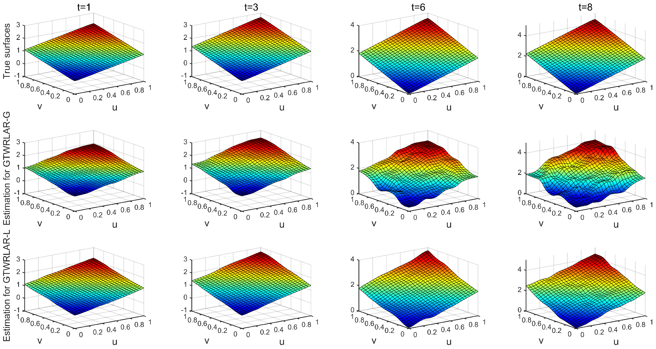
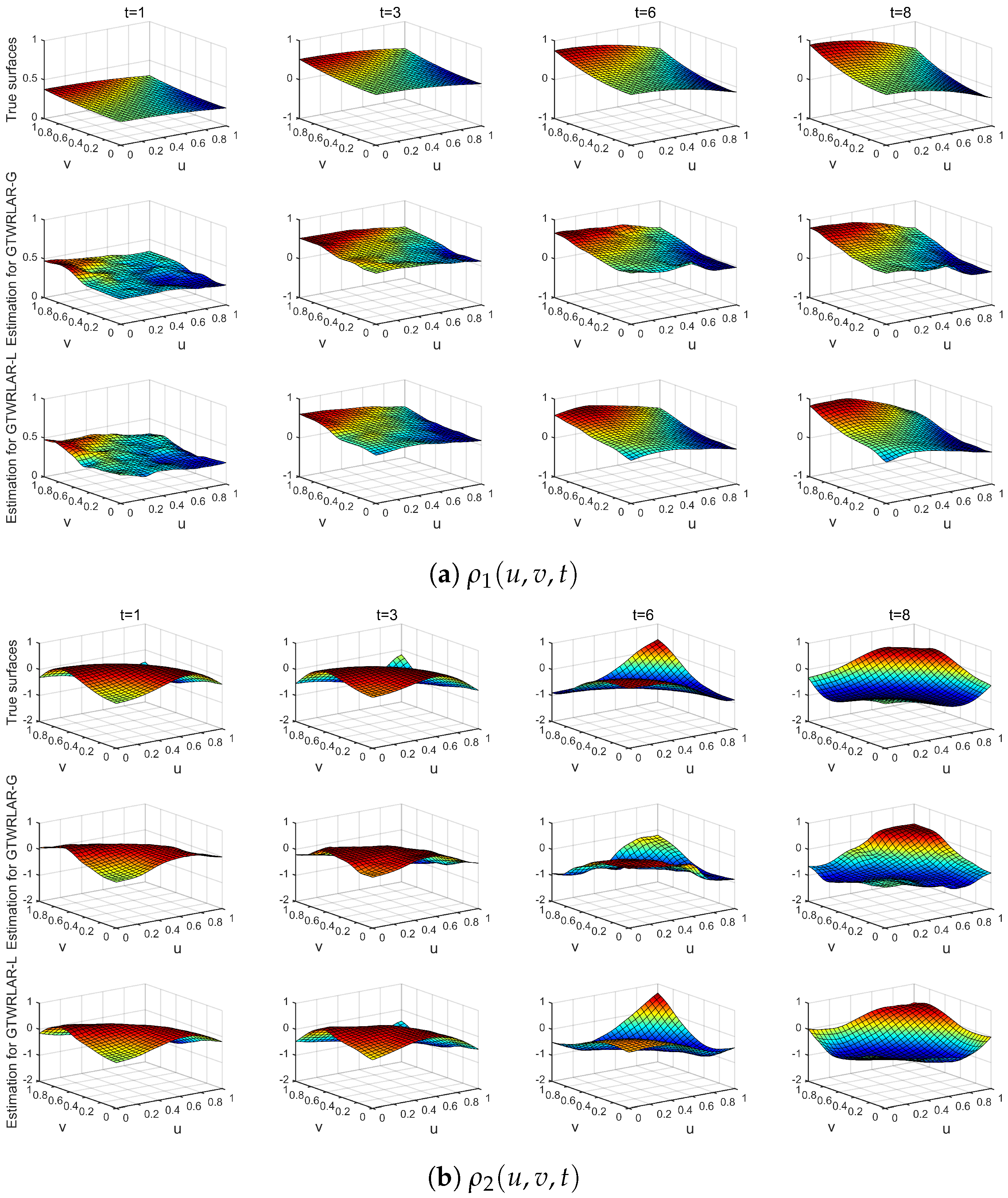
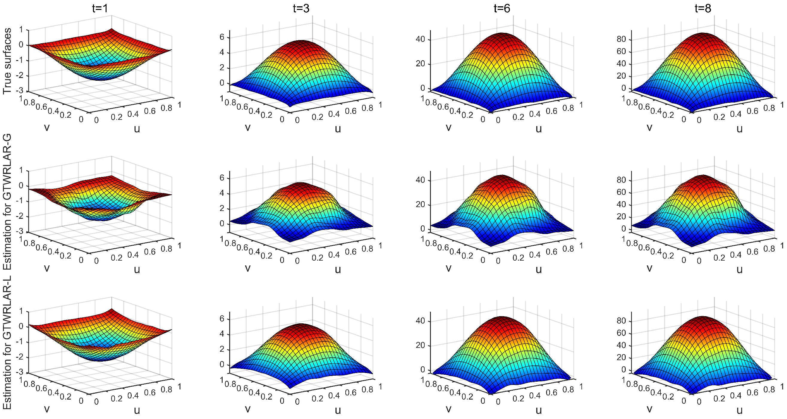
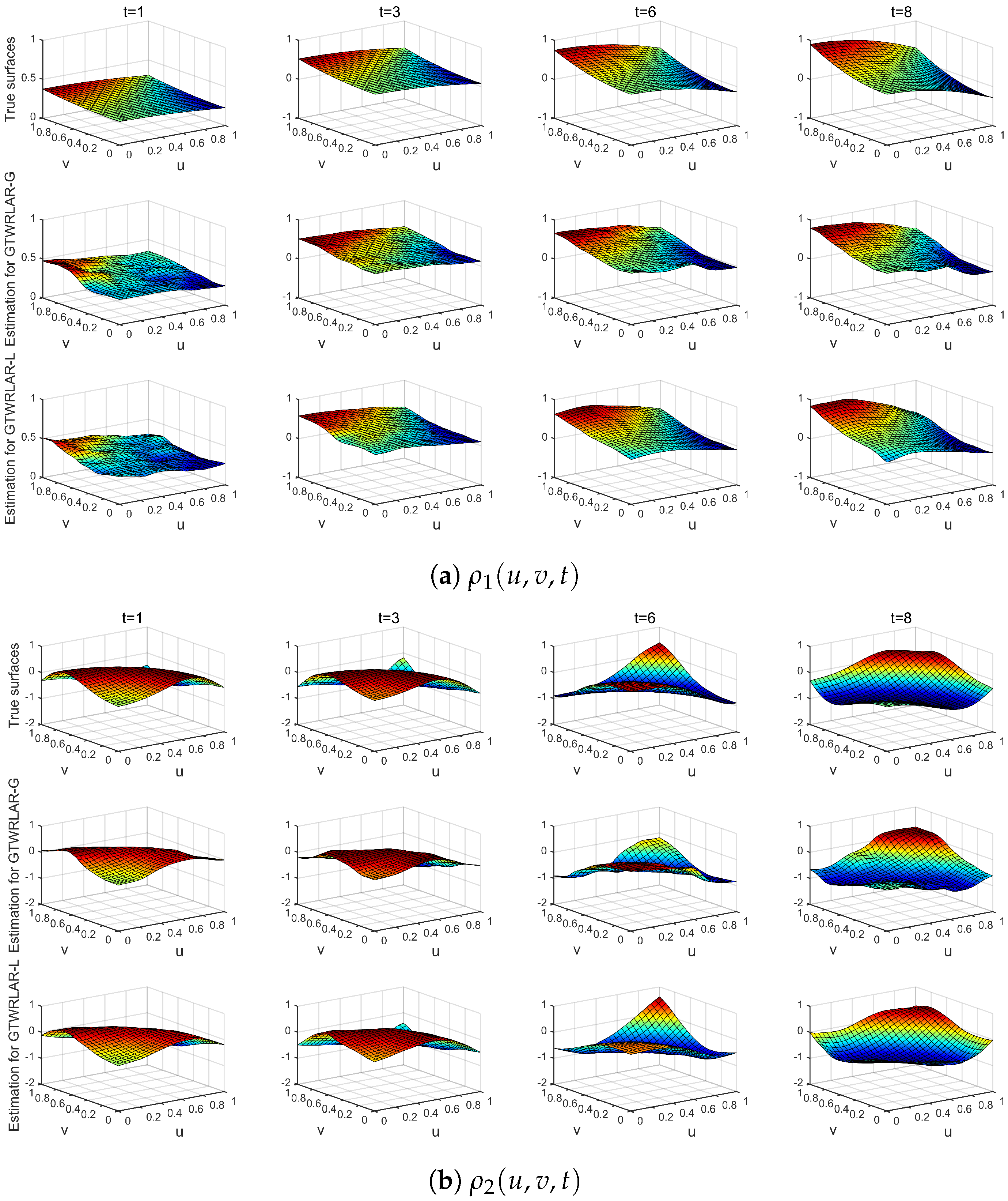
Appendix A.1. The True Surfaces and Estimated Surfaces of the Regression and Autoregressive Coefficients with the Correlation Coefficient Corr = 0.5

Figure A1. The true surfaces and estimated surfaces of the regression coefficient β 1 ( u , v , t ) at different time stamps with the correlation coefficient Corr = 0.5 and the autoregressive coefficient ρ 1 ( u , v , t ) .
Ijgi 14 00276 g0a1
Figure A2. The true surfaces and estimated surfaces of the regression coefficient β 2 ( u , v , t ) at different time stamps with the correlation coefficient Corr = 0.5 and the autoregressive coefficient ρ 1 ( u , v , t ) .
Ijgi 14 00276 g0a2
Figure A3. The true surfaces and estimated surfaces of the regression coefficient β 3 ( u , v , t ) at different time stamps with the correlation coefficient Corr = 0.5 and the autoregressive coefficient ρ 1 ( u , v , t ) .
Ijgi 14 00276 g0a3
Figure A4. The true surfaces and estimated surfaces of the autoregressive coefficients with the correlation coefficient Corr = 0.5 .
Ijgi 14 00276 g0a4

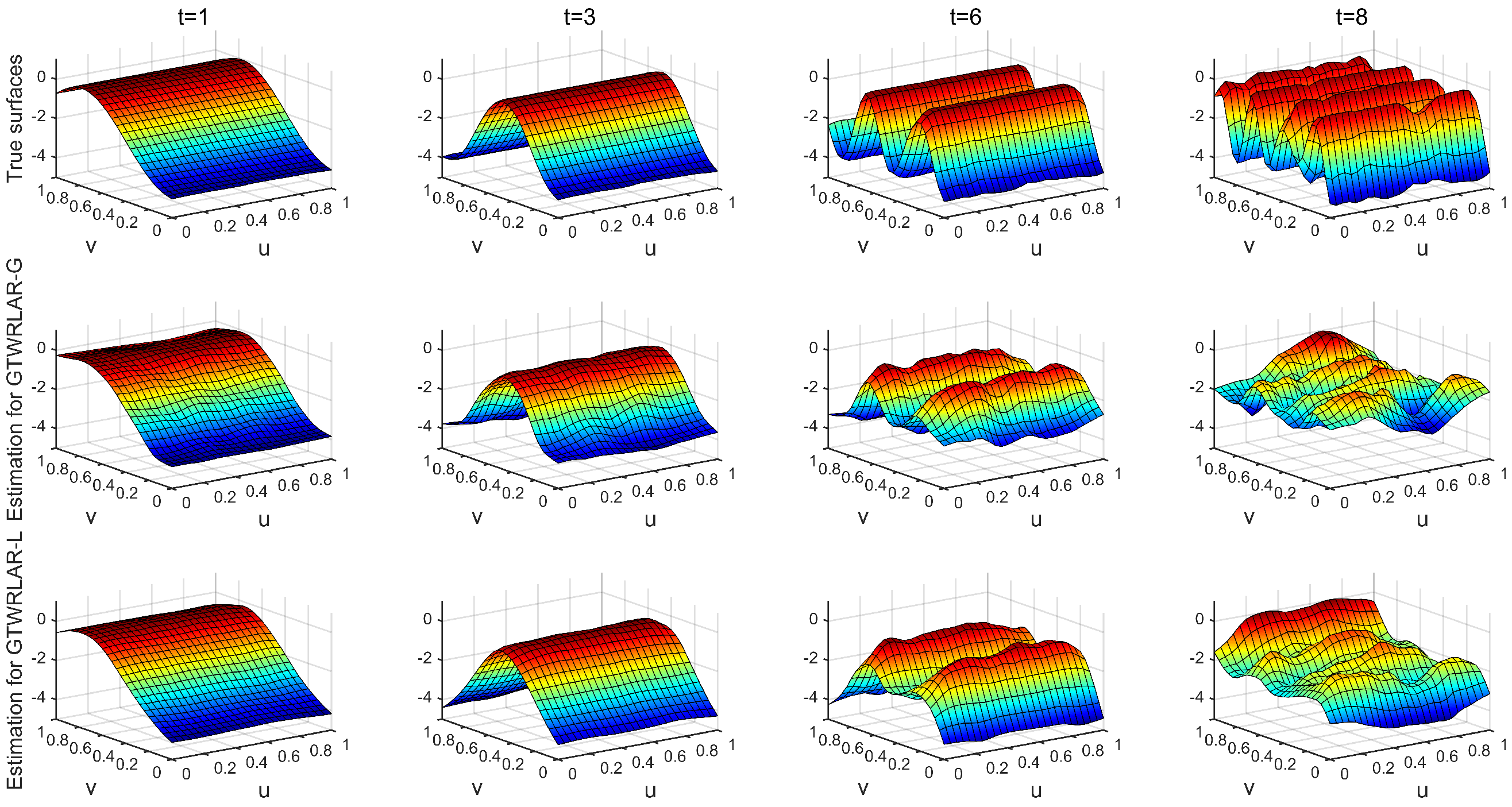
Appendix A.2. The True Surfaces and Estimated Surfaces of the Regression and Autoregressive Coefficients with the Correlation Coefficient Corr = 0.9

Figure A5. The true surfaces and estimated surfaces of the regression coefficient β 1 ( u , v , t ) at different time stamps with the correlation coefficient Corr = 0.9 and the autoregressive coefficient ρ 1 ( u , v , t ) .
Ijgi 14 00276 g0a5
Figure A6. The true surfaces and estimated surfaces of the regression coefficient β 2 ( u , v , t ) at different time stamps with the correlation coefficient Corr = 0.9 and the autoregressive coefficient ρ 1 ( u , v , t ) .
Ijgi 14 00276 g0a6
Figure A7. The true surfaces and estimated surfaces of the regression coefficient β 3 ( u , v , t ) at different time stamps with the correlation coefficient Corr = 0.9 and the autoregressive coefficient ρ 1 ( u , v , t ) .
Ijgi 14 00276 g0a7
Figure A8. The true surfaces and estimated surfaces of the autoregressive coefficients with the correlation coefficient Corr = 0.9 .
Ijgi 14 00276 g0a8

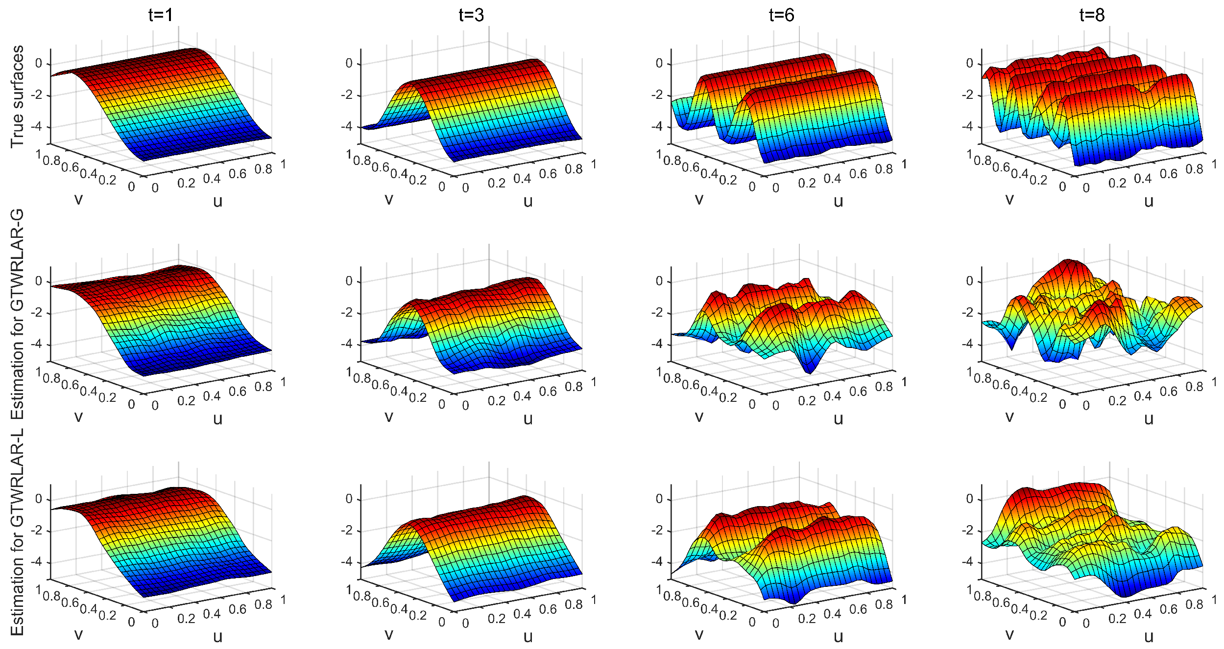
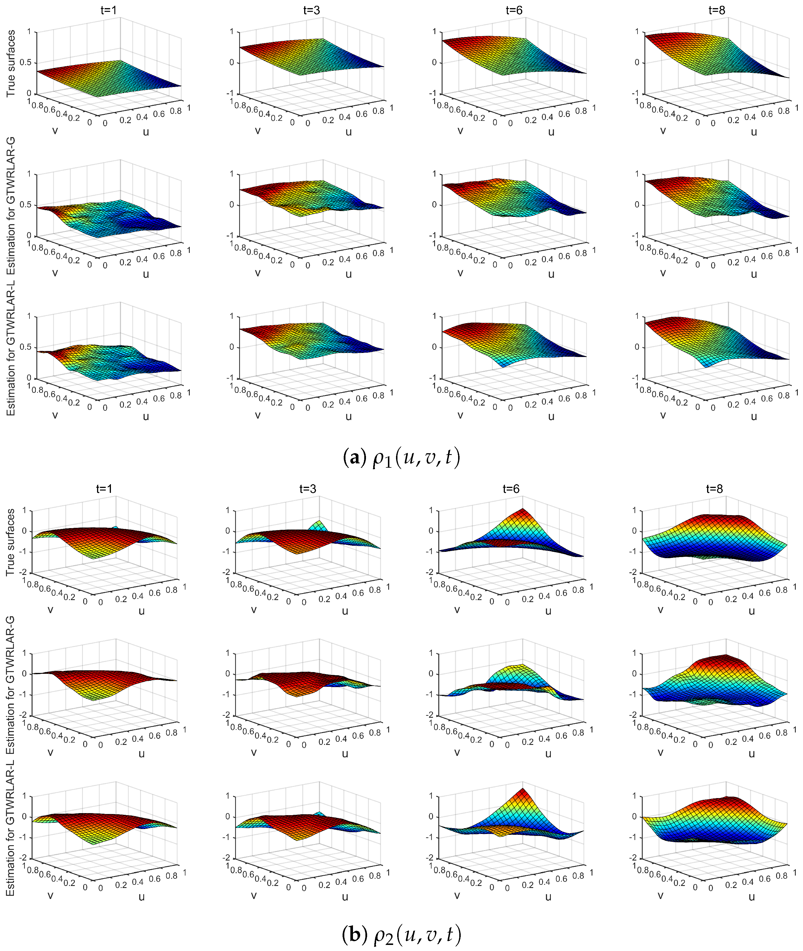
Appendix A.3. The True Surfaces and Estimated Surfaces of the Regression and Autoregressive Coefficients with the Correlation Coefficient Corr = 0.99

Figure A9. The true surfaces and estimated surfaces of the regression coefficient β 1 ( u , v , t ) at different time stamps with the correlation coefficient Corr = 0.99 and the autoregressive coefficient ρ 1 ( u , v , t ) .
Ijgi 14 00276 g0a9
Figure A10. The true surfaces and estimated surfaces of the regression coefficient β 2 ( u , v , t ) at different time stamps with the correlation coefficient Corr = 0.99 and the autoregressive coefficient ρ 1 ( u , v , t ) .
Ijgi 14 00276 g0a10
Figure A11. The true surfaces and estimated surfaces of the regression coefficient β 3 ( u , v , t ) at different time stamps with the correlation coefficient Corr = 0.99 and the autoregressive coefficient ρ 1 ( u , v , t ) .
Ijgi 14 00276 g0a11
Figure A12. The true surfaces and estimated surfaces of the autoregressive coefficients with the correlation coefficient Corr = 0.99 .
Ijgi 14 00276 g0a12aIjgi 14 00276 g0a12b

References

  1. Mcerlean, S.; Patton, M. Spatial Effects within the Agricultural Land Market in Northern Ireland. J. Agric. Econ. 2003, 54, 35–54. [Google Scholar] [CrossRef]
  2. Gray, D. District House Price Movements in England and Wales 1997–2007:An Exploratory Spatial Data Analysis Approach. Urban Stud. 2012, 49, 1411–1434. [Google Scholar] [CrossRef]
  3. Brunsdon, C.; Fotheringham, A.S.; Charlton, M.E. Geographically Weighted Regression: A Method for Exploring Spatial Nonstationarity. Geogr. Anal. 1996, 28, 281–298. [Google Scholar] [CrossRef]
  4. Huang, B.; Wu, B.; Barry, M. Geographically and temporally weighted regression for modeling spatio-temporal variation in house prices. Int. J. Geogr. Inf. Sci. 2010, 24, 383–401. [Google Scholar] [CrossRef]
  5. Fotheringham, A.S.; Crespo, R.; Yao, J. Geographical and Temporal Weighted Regression (GTWR). Geogr. Anal. 2015, 47, 431–452. [Google Scholar] [CrossRef]
  6. Guo, Y.; Tang, Q.; Gong, D.Y.; Zhang, Z. Estimating ground-level PM 2.5 concentrations in Beijing using a satellite-based geographically and temporally weighted regression model. Remote Sens. Environ. 2017, 198, 140–149. [Google Scholar] [CrossRef]
  7. Qiu, Y.; Ma, L.; Ju, T. Independent and compound characteristics of PM2.5, ozone, and extreme heat pollution events in Korea. Environ. Monit. Assess. 2025, 197, 49. [Google Scholar] [CrossRef] [PubMed]
  8. Du, Z.; Wu, S.; Zhang, F.; Liu, R.; Zhou, Y. Extending geographically and temporally weighted regression to account for both spatiotemporal heterogeneity and seasonal variations in coastal seas. Ecol. Inform. 2018, 43, 185–199. [Google Scholar] [CrossRef]
  9. Lacheheb, M.; Noy, I.; Kahui, V. Marine heatwaves and commercial fishing in New Zealand. Sci. Total Environ. 2024, 954, 176558. [Google Scholar] [CrossRef] [PubMed]
  10. Ma, X.; Zhang, J.; Ding, C.; Wang, Y. A geographically and temporally weighted regression model to explore the spatiotemporal influence of built environment on transit ridership. Comput. Environ. Urban Syst. 2018, 70, 113–124. [Google Scholar] [CrossRef]
  11. Bao, J.; Wang, Z.; Yang, Z.; Shan, X. Exploring spatiotemporal patterns and influencing factors of ridesourcing and traditional taxi usage using geographically and temporally weighted regression method. Transp. Plan. Technol. 2023, 46, 1–23. [Google Scholar] [CrossRef]
  12. Ling, L.; Zhang, W.; Bao, J. Influencing factors for right turn lane crash frequency based on geographically and temporally weighted regression models. J. Saf. Res. 2023, 86, 191–208. [Google Scholar] [CrossRef] [PubMed]
  13. Hong, Z.M.; Mei, C.L.; Wang, H.H.; Du, W.L. Spatiotemporal effects of climate factors on childhood hand, foot, and mouth disease: A case study using mixed geographically and temporally weighted regression models. Int. J. Geogr. Inf. Sci. 2021, 35, 1611–1633. [Google Scholar] [CrossRef]
  14. Zheng, T.; Chen, J.; Wu, W.; Ding, J.; Wang, L.; Zhu, Z.; Chen, D. Spatiotemporal association of urban park characteristics and physical activity levels based on GTWR: A serial cross-sectional observational study. J. Urban Manag. 2024, 13, 398–409. [Google Scholar] [CrossRef]
  15. Pace, R.K.; LeSage, J. Spatial Autoregressive Local Estimation. In Recent Advances in Spatial Econometrics; Palgrave Publishers: New York, NY, USA, 2004; pp. 31–51. [Google Scholar]
  16. Geniaux, G.; Martinetti, D. A new method for dealing simultaneously with spatial autocorrelation and spatial heterogeneity in regression models. Reg. Sci. Urban Econ. 2018, 72, 74–85. [Google Scholar] [CrossRef]
  17. Brunsdon, C.; Fotheringham, A.S.; Charlton, M. Spatial nonstationarity and autoregressive models. Environ. Plan. A 1998, 30, 957–973. [Google Scholar] [CrossRef]
  18. Sun, Y.; Yan, H.; Zhang, W.; Lu, Z. A semiparametric spatial dynamic model. Ann. Stat. 2014, 42, 700–727. [Google Scholar] [CrossRef]
  19. Gao, S.J.; Mei, C.L.; Xu, Q.X.; Zhang, Z. Non-Iterative Multiscale Estimation for Spatial Autoregressive Geographically Weighted Regression Models. Entropy 2023, 25, 320. [Google Scholar] [CrossRef] [PubMed]
  20. Mei, C.L.; Chen, F. Detection of spatial heterogeneity based on spatial autoregressive varying coefficient models. Spat. Stat. 2022, 51, 100666. [Google Scholar] [CrossRef]
  21. Wu, B.; Li, R.; Huang, B. A geographically and temporally weighted autoregressive model with application to housing prices. Int. J. Geogr. Inf. Sci. 2014, 28, 1186–1204. [Google Scholar] [CrossRef]
  22. Wand, M.; Jones, M. Kernel Smoothing; Taylor & Francis: Abingdon, UK, 1994. [Google Scholar] [CrossRef]
  23. Wang, N.; Mei, C.L.; Yan, X.D. Local Linear Estimation of Spatially Varying Coefficient Models: An Improvement on the Geographically Weighted Regression Technique. Environ. Plan. A 2008, 40, 986–1005. [Google Scholar] [CrossRef]
  24. Wu, B.; Yan, J.; Lin, H. A cost-effective algorithm for calibrating multiscale geographically weighted regression models. Int. J. Geogr. Inf. Sci. 2022, 36, 898–917. [Google Scholar] [CrossRef]
  25. Fotheringham, A.S.; Brunsdon, C.; Charlton, M. Geographically Weighted Regression: The Analysis of Spatially Varying Relationships; John Wiley & Sons: Chichester, UK, 2002. [Google Scholar]
  26. Boots, B.; Tiefelsdorf, M. Global and Local Spatial Autocorrelation in Bounded Regular Tesselations. J. Geogr. Syst. 2000, 2, 319–348. [Google Scholar] [CrossRef]
  27. Zhao, J.; Liu, Y.; Zhu, Y.; Qin, S.; Wang, Y.; Miao, C. Spatio-temporal patterns and influencing factors of the coupling between new urbanization and ecological environment in the Yellow River Basin. Resour. Sci. 2020, 166, 112300. [Google Scholar]
  28. Xue, M.; Wang, C.; Zhao, J.; Li, M. Spatial and temporal differentiation patterns and influencing factors of tourism economy in the Yellow River Basin. Econ. Geogr. 2020, 40, 21–29. [Google Scholar]
  29. Li, Z.; Ren, L.; Ma, R.; Liu, Y.; Yao, D. Analysis of spatiotemporal pattern and driving factors of carbon emissions in Zhejiang Province based on spatiotemporal geographically weighted regression model. J. Ningbo Univ. Nat. Sci. Eng. Ed. 2021, 80, 414–428. [Google Scholar]
  30. Jia, J.; Tian, S.; Jiang, E.; Liang, S.; Zhao, Q.; Zou, Q.; Chen, R.; Zhang, Y. Research on carbon emission status in the Yellow River Basin and the path to achieve the “dual carbon” goal. People’s Yellow River 2023, 45, 8–13. [Google Scholar]
  31. Gao, X.; Han, X. Research on spatial differentiation and influencing factors of carbon emissions in the Yellow River Basin. Econ. Surv. 2022, 39, 13–23. [Google Scholar] [CrossRef]
  32. Wu, J.R. Spatiotemporal evolution, spatial spillover effect and influencing factors of carbon emissions: An empirical study based on 79 cities in central China. China Collect. Econ. 2023, 36, 104–107. [Google Scholar]
  33. Jin, F. Research on the impact of urbanization on carbon emissions and spatial spillover effect in China. Technol. Innov. Manag. 2023, 44, 220–227. [Google Scholar] [CrossRef]
  34. Wang, Q.; Cui, L.; Yan, H. Spatial heterogeneity of influencing factors of regional economic differences in the Yellow River Basin: An empirical study based on the MGWR model. Areal Res. Dev. 2023, 42, 7–13. [Google Scholar]
  35. Chen, F.; Leung, Y.; Mei, C.L.; Fung, T. Backfitting Estimation for Geographically Weighted Regression Models with Spatial Autocorrelation in the Response. Geogr. Anal. 2021, 54, 357–381. [Google Scholar] [CrossRef]
  36. Wei, C.H.; Wang, S.J.; Su, Y.N. Local GMM estimation of geographically weighted autoregressive models with spatially varying coefficients. Stat. Inf. Forum 2022, 37, 3–13. [Google Scholar]
  37. Li, D.K.; Mei, C.L.; Wang, N. Tests for spatial dependence and heterogeneity in spatially autoregressive varying coefficient models with application to Boston house price analysis. Reg. Sci. Urban Econ. 2019, 79, 103470. [Google Scholar] [CrossRef]
Figure 1. Box plots of RMSEs for autoregressive and regression coefficients in GTWRLAR models under four collinearity levels of explanatory variables.
Ijgi 14 00276 g001
Figure 2. The true surfaces and estimated surfaces of the regression coefficient β 1 ( u , v , t ) at different time stamps when the correlation coefficient Corr = 0 and the autoregressive coefficient is ρ 1 ( u , v , t ) .
Ijgi 14 00276 g002
Figure 3. The true surfaces and estimated surfaces of the regression coefficient β 2 ( u , v , t ) at different time stamps when the correlation coefficient Corr = 0 and the autoregressive coefficient is ρ 1 ( u , v , t ) .
Ijgi 14 00276 g003
Figure 4. The true surfaces and estimated surfaces of the regression coefficient β 3 ( u , v , t ) at different time stamps with the correlation coefficient Corr = 0 and the autoregressive coefficient ρ 1 ( u , v , t ) .
Ijgi 14 00276 g004
Figure 5. The true surfaces and estimated surfaces of the autoregressive coefficients with the correlation coefficient Corr = 0 .
Ijgi 14 00276 g005
Figure 6. Scatter plot of Moran’s I for all data.
Ijgi 14 00276 g006
Figure 7. Maps of the GTWRLAR-L estimators of the autoregressive coefficient (a) ρ ( u , v , t ) and the spatiotemporally varying coefficients, (b) β 1 ( u , v , t ) (GDP), (c) β 2 ( u , v , t ) (IIR), (d) β 3 ( u , v , t ) (PP), (e) β 4 ( u , v , t ) (UR), (f) β 5 ( u , v , t ) (SDE), (g) β 6 ( u , v , t ) (DPE), and (h) β 7 ( u , v , t ) (SWDR), in Yellow River Basin carbon emission study (2017–2021).
Ijgi 14 00276 g007
Table 1. Summary statistics of the optimal spatiotemporal bandwidths, RSS, and AIC c values of the simulated data in 200 replications.
CoefficientsCorrMethodBandwidths/Ind.MinQ1MedianQ3Max
ρ 1 ( u , v , t ) 0.0GTWRLAR - G ( k , h T ) ( 185 , 1 ) ( 212 , 1 ) ( 212 , 1 ) ( 227 , 1 ) ( 253 , 1 )
RSS20,54324,83525,99428,02033,078
AICc3.9684.0874.1214.1554.262
GTWRLAR - L ( k , h T ) ( 253 , 1 ) ( 297 , 2 ) ( 299 , 2 ) ( 306 , 2 ) ( 329 , 2 )
RSS37174805505253496322
AICc2.5382.6302.6692.7082.902
0.5GTWRLAR - G ( k , h T ) ( 185 , 1 ) ( 212 , 1 ) ( 212 , 1 ) ( 227 , 1 ) ( 253 , 1 )
RSS20,74924,96426,13527,55433,457
AICc3.9754.0934.1274.1634.267
GTWRLAR - L ( k , h T ) ( 253 , 1 ) ( 297 , 2 ) ( 306 , 2 ) ( 306 , 2 ) ( 329 , 2 )
RSS36074687497752586003
AICc2.5172.6032.6422.6842.893
0.9GTWRLAR - G ( k , h T ) ( 185 , 1 ) ( 212 , 1 ) ( 212 , 1 ) ( 227 , 1 ) ( 253 , 1 )
RSS21,16425,13526,57227,93134,144
AICc3.9934.1084.1414.1784.281
GTWRLAR - L ( k , h T ) ( 253 , 1 ) ( 293 , 2 ) ( 299 , 2 ) ( 306 , 2 ) ( 329 , 2 )
RSS36134768502252906104
AICc2.5452.6172.6562.6952.917
0.99GTWRLAR - G ( k , h T ) ( 185 , 1 ) ( 212 , 1 ) ( 212 , 1 ) ( 220 , 1 ) ( 253 , 1 )
RSS21,48025,38326,79028,25334,669
AICc4.0064.1214.1534.1924.292
GTWRLAR - L ( k , h T ) ( 253 , 1 ) ( 293 , 2 ) ( 297 , 2 ) ( 306 , 2 ) ( 329 , 2 )
RSS36854834511354176424
AICc2.5612.6382.6782.7172.943
ρ 2 ( u , v , t ) 0.0GTWRLAR - G ( k , h T ) ( 162 , 1 ) ( 212 , 1 ) ( 212 , 1 ) ( 220 , 1 ) ( 253 , 1 )
RSS20,26328,26729,43031,02238,692
AICc4.1134.2344.2674.3044.393
GTWRLAR - L ( k , h T ) ( 282 , 1 ) ( 310 , 2 ) ( 324 , 2 ) ( 324 , 2 ) ( 347 , 2 )
RSS56557011746179649167
AICc2.8092.9252.9592.9913.108
0.5GTWRLAR - G ( k , h T ) ( 162 , 1 ) ( 212 , 1 ) ( 212 , 1 ) ( 219 , 1 ) ( 253 , 1 )
RSS20,36628,22829,43130,93936,818
AICc4.1174.2414.2714.3094.397
GTWRLAR - L ( k , h T ) ( 282 , 1 ) ( 306 , 2 ) ( 324 , 2 ) ( 324 , 2 ) ( 347 , 2 )
RSS51756836734578299016
AICc2.7932.9082.9392.9703.080
0.9GTWRLAR - G ( k , h T ) ( 162 , 1 ) ( 212 , 1 ) ( 212 , 1 ) ( 212 , 1 ) ( 253 , 1 )
RSS20,65028,60929,85131,24538,654
AICc4.1334.2564.2844.3234.423
GTWRLAR - L ( k , h T ) ( 282 , 1 ) ( 306 , 2 ) ( 315 , 2 ) ( 324 , 2 ) ( 347 , 2 )
RSS51906887746378749976
AICc2.8112.9182.9522.9843.094
0.99GTWRLAR - G ( k , h T ) ( 162 , 1 ) ( 212 , 1 ) ( 212 , 1 ) ( 212 , 1 ) ( 253 , 1 )
RSS20,89328,79630,12831,60439,222
AICc4.1454.2674.2954.3344.440
GTWRLAR - L ( k , h T ) ( 274 , 1 ) ( 306 , 2 ) ( 315 , 2 ) ( 324 , 2 ) ( 333 , 2 )
RSS52736925745179919169
AICc2.8302.9372.9723.0033.113
Table 2. Spatial autocorrelation analysis of carbon emissions in the Yellow River Basin from 2017 to 2021.
YearMoran’s IZ-Valuep-Value
20170.7199.6510.000
20180.6368.5660.000
20190.6819.1520.000
20200.7389.9090.000
20210.6809.1620.000
Table 3. Diagnostic information for GTWR, GTWRLAR-G, and GTWRLAR-L.
h S h T R 2 RSS AIC c
GTWR8250.87150.3420.143
GTWRLAR-G12450.88843.411−0.363
GTWRLAR-L29950.89341.495−0.101
Table 4. The distributions of the GTWRLAR-L spatiotemporally varying coefficient estimates.
MinQ1MedianQ3Max
CE (10,000 tons): ρ ( u i , v i , t l ) 0.4560.9521.0591.2842.284
GDP (yuan): β 1 ( u i , v i , t l ) −2.473−1.039−0.446−0.2610.133
IIR (%): β 2 ( u i , v i , t l ) −0.3300.0510.1780.3881.084
PP: β 3 ( u i , v i , t l ) −0.545−0.0170.0440.1841.043
UR (%): β 4 ( u i , v i , t l ) −0.2590.1780.3680.6991.522
SDE (tons): β 5 ( u i , v i , t l ) −1.369−0.139−0.0240.0400.531
DPE (tons): β 6 ( u i , v i , t l ) −0.570−0.104−0.0110.1231.070
SWDR (%): β 7 ( u i , v i , t l ) −0.0340.0990.2920.6342.656
Disclaimer/Publisher’s Note: The statements, opinions and data contained in all publications are solely those of the individual author(s) and contributor(s) and not of MDPI and/or the editor(s). MDPI and/or the editor(s) disclaim responsibility for any injury to people or property resulting from any ideas, methods, instructions or products referred to in the content.

