SP-GEM: Spatial Pattern-Aware Graph Embedding for Matching Multisource Road Networks

Abstract

Identifying correspondences of road segments in different road networks, namely road-network matching, is an essential task for road network-centric data processing such as data integration of road networks and data quality assessment of crowd-sourced road networks. Traditional road-network matching usually relies on feature engineering and parameter selection of the geometry and topology of road networks for similarity measurement, resulting in poor performance when dealing with dense and irregular road network structures. Recent development of graph neural networks (GNNs) has demonstrated unsupervised modeling power on road network data, which learn the embedded vector representation of road networks through spatial feature induction and topology-based neighbor aggregation. However, weighting spatial information on the node feature alone fails to give full play to the expressive power of GNNs. To this end, this paper proposes a Spatial Pattern-aware Graph EMbedding learning method for road-network matching, named SP-GEM, which explores the idea of spatially-explicit modeling by identifying spatial patterns in neighbor aggregation. Firstly, a road graph is constructed from the road network data, and geometric, topological features are extracted as node features of the road graph. Then, four spatial patterns, including grid, high branching degree, irregular grid, and circuitous, are modelled in a sector-based road neighborhood for road embedding. Finally, the similarity of road embedding is used to find data correspondences between road networks. We conduct an algorithmic accuracy test to verify the effectiveness of SP-GEM on OSM and Tele Atlas data. The algorithmic accuracy experiments show that SP-GEM improves the matching accuracy and recall by at least 6.7% and 10.2% among the baselines, with high matching success rate (>70%), and improves the matching accuracy and recall by at least 17.7% and 17.0%, compared to the baseline GNNs, without spatially-explicit modeling. Further embedding analysis also verifies the effectiveness of the induction of spatial patterns. This study not only provides an effective and practical algorithm for road-network matching, but also serves as a test bed in exploring the role of spatially-explicit modeling in GNN-based road network modeling. The experimental performances of SP-GEM illuminate the path to develop GeoEmbedding services for geospatial applications.

1. Introduction

The road network, being an essential component of urban infrastructure, has valuable applications in many fields such as traffic management and urban planning. To ensure that road network data can reflect the infrastructure changes in a timely manner, each department collects and produces road network data with different times and specifications, according to its own needs. This has led to large differences in road network data from different sources, which cannot fully meet the practical needs of real-world applications. Therefore, it is necessary to match these road network data from different sources [1], i.e., to identify the correspondence of road segments between different datasets, which plays an important role in monitoring and updating of road network changes and assessment of road network data quality [2].

Traditional road-network matching methods fall into three categories, namely geometry-based, semantic-based, and advanced algorithms. Geometric matching algorithms achieve road-network matching by comparing the distance, shape and topological similarity of road segments [3,4]. Semantic matching algorithms, on the other hand, focus on analyzing the similarity of semantic attributes of road networks [5,6]. Advanced matching algorithms, such as ICP [7], BG [8] and limited stroke algorithm [9], improve the matching accuracy by integrating the geometric and topological information of roads and optimization strategies. However, these methods are still constrained by factors such as road network complexity [10,11]. Chen et al. [12] propose a method that integrates semantic, geometric and topological information, achieving good experimental results while requiring high data integrity. The road-network matching algorithm using fuzzy hierarchy theory requires precise road classification, and the matching accuracy decreases when semantic information is missing [13]. In conclusion, traditional road-network matching algorithms rely on manually extracted features for similarity measures and are limited by prior knowledge of parameter selection and the need for high-quality data, which means their performance struggles when dealing with dense and irregular road network structures. Recent road-network matching methods have evolved towards integrating local and global features, and have not been able to effectively overcome the above problems, despite the development of more advanced similarity measures [14,15].

Deep learning techniques, especially graph neural networks (GNNs), have made remarkable progress in the field of graph data processing. GNNs can effectively model complex topologies and dependencies between graph nodes, and have been widely used in fields such as social network link prediction [16] and molecular structure modeling [17]. In geospatial data modeling, Wang et al. [18] characterized the road network data as an undirected planar graph, and extracted the graph node features of the roads through the linear road sectioning method for road network pattern recognition. Zhang et al. [19] proposed a spatio-temporal generative adversarial clustering graph convolution network, which effectively captures the long-term temporal dependencies of traffic flows by mining the short-term spatio-temporal features of the traffic flows and combining them with the long short-term memory network module, thus achieving significant improvements in anomalous traffic flow prediction. Yu et al. [20] designed a graph convolutional network-based method for drainage network pattern recognition by constructing a water-network dual graph and extracting water network features at three different scales as inputs. Yang et al. [21] proposed a semi-supervised method based on shape context features and graph convolutional networks for recognizing complex interchange patterns, which improves the accuracy of identifying road interchanges.

Since GNNs perform well in spatial networks, especially road network modeling, this provides important insights for road-network matching. Soni et al. [22] proposed a similarity-based matching algorithm based on node embeddings of heterogeneous geospatial graphs, which uses GraphSAGE for neighbor sampling and aggregation to compute the node embeddings for similarity measure. Gadi et al. [23] extracted the geometric, topological, and semantic features of each road segment after preprocessing the road network data such as stroke extraction. Then the geometric features were resampled and encoded into a 1024-dimension vector, while the semantic and topological features were encoded into 768 dimensions using BERT, respectively. The final road embedding is calculated as the weighted sum of the three feature vectors for road-network matching. Yang et al. [24] introduced a spatial relationship and semantic relationship into GNNs’ neighbor aggregation, which improve the expressivity of the graph representation of road network data and the overall task performance of the road-network matching.

Although all the above-mentioned methods have made progress in road-network matching, there is still a need to improve the overall algorithmic accuracy for real-world applications. The significant improvement made by modeling spatial context in GNNs’ neighbor aggregation has paved the way for further investigation in modeling spatial patterns of the road network to enhance task performance [24]. Urban road networks exhibit diverse spatial structures. For example, the road network in Beijing integrates ring and grid structures, and the interweaving of ring roads and radial arterial roads forms a unique spatial hierarchy; the road network structure in Singapore shows a clear hierarchy that reveals functional zoning of the arterial road network and the secondary road network; the shape of the road network in Rio de Janeiro is more constrained by the mountainous terrain, and results in a curved structure aligned with contours. The diverse spatial patterns in the road networks make it difficult to derive a discriminative representation of road networks, thus affecting the matching performance. On the other hand, spatial patterns are less sensitive to local variances in the road network, and the overall spatial distribution of the road network remains stable, even if local connectivity changes, thus providing a more reliable feature for matching. Therefore, it is promising to incorporate a spatial pattern into the framework of GNNs for road-network matching.

This paper proposes a Spatial Pattern-aware Graph EMbedding method for road-network matching (SP-GEM), which explicitly models the distribution of spatial patterns in graph nodes’ neighbor aggregation to enhance the graph embedding’s expressivity, and thus improve the performance of GNNs for road-network matching. The contributions of this paper mainly include the following:

(1) We propose a spatial pattern-aware graph embedding method for road-network matching, which updates node embedding by explicitly modeling the spatial distribution of four types of spatial structures in a road network, to obtain more discriminative data embedding for road-network matching.

(2) We validated the accuracy of our method using Ansbach’s road network from OpenStreetMap (OSM) and Tele Atlas. The experiment results show that the proposed method improves the matching precision and recall by at least 6.7% and 10.2%, with a high matching rate (>70%), respectively; and it achieves at least 17.7% and 17.0% improvement in precision and recall compared to the plain GNNs-based methods.

(3) We analyzed SP-GEM road network embeddings to verify the effects of spatial pattern modeling on the model’s performance. As shown in the analysis, such efforts not only improve the model’s classification capability of road patterns, but are also helpful for the contextual modeling for computing road embeddings.

The remainder of the paper is organized as follows. Section 2 describes the overall framework and the key designs of the proposed road-network matching method, Section 3 gives the experimental results and the experimental analyses, and Section 4 validates the effectiveness of the proposed method through feature ablation experiments. The last section gives the conclusions.

2. Method

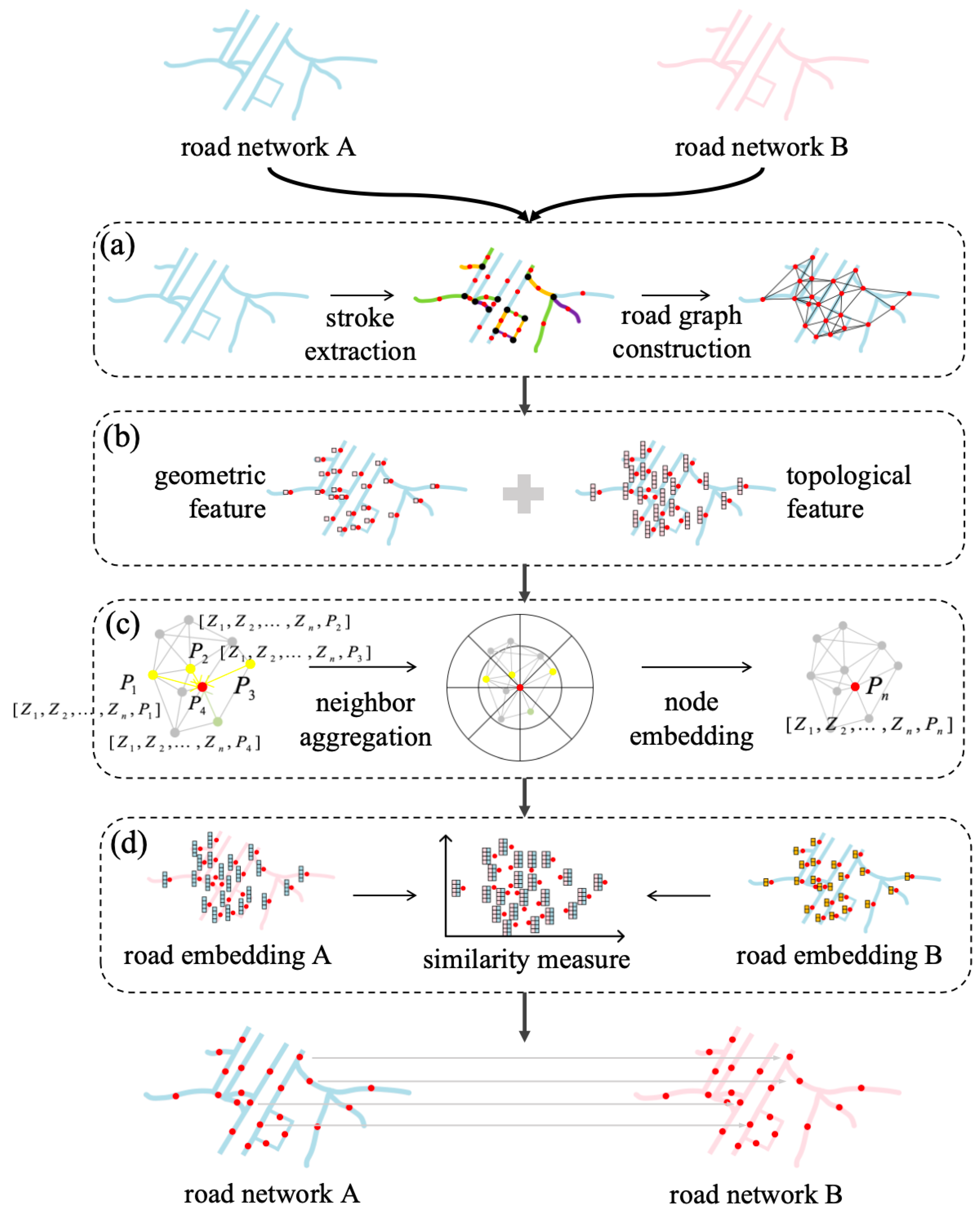
2.1. Methodology Framework

In this paper, we use GNNs to learn the vector representation of road network data, and infer the correspondences between road segments using node embedding for matching road network data from different sources. Inspired by the graph embedding-based road-network matching [22,24], the proposed work develops a novel neighbor aggregation that captures the spatial structures of the road network, named SP-GEM, which significantly improves the model performance of the road-network matching task. As shown in Figure 1, the framework of the proposed method includes four steps:

(1) Road graph construction. We first preprocessed road network data and performed stroke extraction, then constructed a road graph with nodes of processed road segments and edges between roads, within predefined spatial proximity.

(2) Road graph feature extraction. We extracted geometric and topological features of road segments, such as geometric morphology, MBR aspect ratio, etc. Leaving out semantic features helps to reduce model dependence on the likely missing road attributes in the open-sourced road network data.

(3) Spatial Pattern-aware Road Embedding. Four spatial patterns, i.e., Grid, High branching degree, Irregular grid, and Circuitous, were modelled, based on GraphSAGE’s neighbor aggregation to update node embedding, which improved the model’s expressivity in representing complex road network structures.

(4) Similarity measure based on road embedding. For road network data from different sources, we first computed the graph node embedding of road network data separately, and calculated the similarity of road segments from different data sources to determine road segments’ correspondences.

2.2. Road Graph Construction

Road network data is usually represented by a graph model, and we use an undirected spatial proximity graph to construct a road graph for road network data. Firstly, the road network data are preprocessed for noise removal and stroke extraction [24]. Then, the midpoint of the stroke road segment is selected as the node of the road graph. With each node as the center, a buffer with a radius of Euclidean distance M is established for find nodes within proximity to establish graph edges, which obtain the road graph $G=(V,E)$, where $V,E$ are the sets of nodes and edges, respectively.

2.3. Feature Extraction

After constructing the road graph, graph node features need to be extracted and used as inputs for graph representation learning. The matching of the road network not only depends on the geometric features of the road segments (e.g., aspect ratio, direction of the minimum bounding rectangle (MBR)), but also needs to consider the topological features (e.g., average node degree) of the nodes [20,22,25].

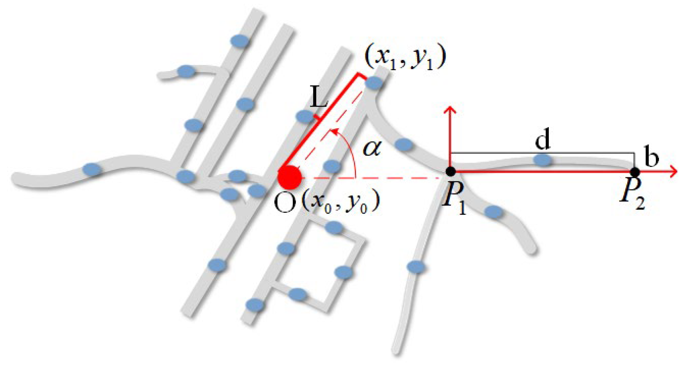
2.3.1. Geometric Feature

The geometric features of the road segments consist of eight numerical indicators, which are divided into three categories: MBR features, center point features, and structural features. Further details are provided below. Additionally, schematic diagrams and formula explanations for the relevant feature calculations are presented, as shown in Figure 2 and

Table 1. Geometric features of a road segment.

Category	Feature	Equation
MBR feature	Length-to-width ratio of the MBR	$d/b$ $d$: The longer side of the MBR $b$: The shorter side of the MBR
	Direction of the longest side of the MBR	${\mathrm{atan}2(\mathrm{P}}_{\mathrm{y}2}-P_{y1},P_{x_2}-P_{x1})$ $P_{y2}$$: \mathrm{The} \mathrm{latitude} \mathrm{of} \mathrm{the} \mathrm{point} P_2$ $P_{x2}$$: \mathrm{The} \mathrm{longitude} \mathrm{of} \mathrm{the} \mathrm{point} P_2$ $P_{y1}$$: \mathrm{The} \mathrm{latitude} \mathrm{of} \mathrm{the} \mathrm{point} P_1$ $P_{x1}$$: \mathrm{The} \mathrm{longitude} \mathrm{of} \mathrm{the} \mathrm{point} P_1$
Center point feature	Center distance	${\tan }^{-1}{\displaystyle \frac{y_1-y_0}{{\mathrm{x}}_1-x_0}}$ $y_1$: The latitude of the midpoint $x_1$: The longitude of the midpoint $y_0$: The latitude of the center point O $x_0$: The longitude of the center point O
	Centre direction	$\sqrt{{(x_0-x_1)}^2+{(y_0-y_1)}^2}$ $y_1$: The latitude of the midpoint $x_1$: The longitude of the midpoint $y_0$: The latitude of the center point O $x_0$: The longitude of the center point O
Structural feature	Log circuity (r ≤ 500 m)	$\log ({\displaystyle \frac{{\displaystyle \sum D_{sp}}}{{\displaystyle \sum D_{sl}}}})$ $D_{sp}$: The total length of the shortest paths between all pairs of nodes $D_{sl}$: The total straight-line distances between all pairs of nodes
	Log circuity (r > 500 m)	$\log ({\displaystyle \frac{{\displaystyle \sum D_{sp}}}{{\displaystyle \sum D_{sl}}}})$ $D_{sp}$: The total length of the shortest paths between all pairs of nodes $D_{sl}$: The total straight-line distances between all pairs of nodes
	Bridge-edge–length ratio	${\displaystyle \frac{{\displaystyle \sum L_{be}}}{{\displaystyle \sum L_{all}}}}$ $L_{be}$: The total length of edges classified as bridge edges in the graph $L_{all}$: The total length of all edges in the graph
	End-edge–length ratio	${\displaystyle \frac{{\displaystyle \sum L_{ee}}}{{\displaystyle \sum L_{all}}}}$ $L_{ee}$: The total length of edges classified as end edges in the graph $L_{all}$: The total length of all edges in the graph

Note: An edge is called a ‘bridge edge’ if, and only if, its removal increases the number of connected components in the network. An edge is called an ‘end edge’ if, and only if, one of its endpoints has a degree of 1.

.

(1)

MBR feature

• Length-to-width ratio of the MBR is the aspect ratio of the geometric shape of the road segments, which quantifies the slenderness of the road, while identifying patterns of shapes and morphology of road segments.
• Direction of the longest side of the MBR is the angle between the longest side of the MBR and the due-north direction, which portrays the dominant direction of the road.

(2)

Center point feature

• Centre distance is the Euclidean distance between the midpoint of the neighboring road segment and the central road node, which quantifies the location relationship of the road segment and helps to analyze the spatial distribution and layout characteristics of the road network.
• Centre direction is the azimuth from the midpoint of a neighboring road segment to the central node of the road network, portraying the spatial distribution of roads and helping to identify radial structures and directional patterns.

(3)

Structural feature

• Log circuity is the ratio of the perimeter of a road segment’s spiral structure to its straight-line distance, reflecting the road network’s ability to adapt in elevated terrain. The feature with a value greater than 500 m indicates a loose spatial structure, while less than or equal to 500 m shows a compact, highly centralized network layout.
• Bridge-edge length ratio is the ratio of the bridge-edge segment’s length to the road network’s total length, reflecting the degree of dependence and connectivity relationships of key connections in the road network.
• End-edge length ratio is the ratio of the end-edge segment’s length to the road network’s total length, reflecting the degree of branching and structural integrity of the road network.

In addition to the above geometric features, this paper also uses LSTM autoencoder [22] to encode the geometry of road segments, transforming road segments with varying length into 128-dimensional vectors and stacking them with the above-defined geometric features, to obtain the final geometric features.

2.3.2. Topological Feature

The topological features of a road segment refer to a series of indicators that quantitatively characterize the structure of the road network based on graph theory, which uses topological parameters such as node degree, average node degree, etc. The descriptions of these indicators are listed below.

The topological features of the road segments consist of eight numerical indicators, which are divided into two categories, i.e., ratio of node degree feature and structural features. Further details are provided below, and their calculation methods are shown in

Table 2. Topological features of a road segment.

Category	Feature	Equation
Ratio of node-degree feature	Node degree	-
	Average node degree	$S_d/S_n$ $S_d$: Sum of degree for all nodes $S_n$: Number of nodes
	Ratio of nodes with degree of 1	$S_{\mathrm{d}=1}/S_n$ $S_{d=1}$: Number of nodes with degree of 1 $S_n$: Number of nodes
	Ratio of nodes with degree of 2	$S_{d=2}/S_n$ $S_{d=2}$: Number of nodes with degree of 2 $S_n$: Number of nodes
	Ratio of nodes with degree of 3	$S_{d=3}/S_n$ $S_{d=3}$: Number of nodes with degree of 3 $S_n$: Number of nodes
	Ratio of nodes with degree greater than or equal to 4	$S_{d\ge 4}/S_n$ $S_{d\ge 4}$: Number of nodes with degree greater than or equal to 4 $S_n$: Number of nodes
Structural feature	Bridge-edge ratio	$S_{be}/S_{ae}$ $S_{be}$: Number of bridge-edge segments $S_{ae}$: Number of edges
	End-edge ratio	$S_{ee}/S_{ae}$ $S_{ee}$: Number of end-edge segments $S_{ae}$: Number of edges

Note: See Table 1 for the definition of bridge edge and end edge.

.

(1)

Ratio of node degree features

• Node degree is the count of the road segments directly connected to the target road segment, indicating the connectivity complexity and the density of the local road network.
• Ratio of nodes with degree of k is the proportion of road segments connected with only k road segments in the road network. When k = 1, the feature indicates the distribution of end edges and the openness of the network; when k = 2, the feature indicates the linear continuity of the network and the distribution of transmission-type road segments; when k = 3, the feature indicates the distribution of intersections and the underlying branching structure of the road network; and when k ≥ 4, the feature indicates the distribution of complex intersections and the advanced connectivity structure.

(2)

Structural features

• Bridge-edge ratio indicates the proportion of bridge-edge segments in the road network, indicating the distribution density of the key connectivity edge and the connectivity dependency of the road network.
• End-edge ratio indicates the proportion of end-edge segments in the road network, indicating the degree of openness and the boundary characteristics of the road network.

2.4. Spatial Pattern-Aware Road Embedding

Road graph construction and road graph feature extraction transform road network data into feature inputs of GNNs. To obtain an effective road network graph representation, we need to choose a graph embedding framework to compute road embeddings. For road-network matching, the GNN framework should be capable of processing road networks across a wide range of regions exhibiting varying topology. Therefore, this paper adopts the inductive GNNs, GraphSAGE, as the backbone architecture of the model, and proposes a novel neighbor aggregation function to improve the expressivity of the road-network graph embedding.

2.4.1. GraphSAGE Framework

The GraphSAGE framework computes node embeddings through neighbor sampling and aggregating. Specifically, the neighbor aggregation first applies a random walk algorithm for neighbor node sampling, which randomly selects a certain number of neighbor nodes. Then, an aggregation function is applied to the features of the sampled neighbor nodes to update node embeddings. The computation of node embeddings runs iteratively for all nodes in the graph, until a predefined aggregation depth is reached.

The equation of GraphSAGE’s node-embedding update can be written as

$$h_v^k=\sigma (W\cdot [\underset{u\in N(v)}{\mathrm{AGG}}(\{h_v^{k-1},h_u^{k-1}\})])$$

(1)

where $h_v^k$ is the node-embedding vector of node $v$ at layer $k$, $N\left(v\right)$ are the neighbor nodes of node $v$, $W$ is a learnable weight, $\mathsf{\sigma }$ is the activation function, and $\mathrm{A}\mathrm{G}\mathrm{G}(·)$ is an aggregation function that may use aggregation operations such as mean and max pooling.

The GraphSAGE framework can be trained using a unsupervised learning procedure. With the road graph and road features as input, it performs neighbor sampling and feature aggregation to compute node embedding. During the training process, the model computes loss function to iteratively optimize the network parameters based on the back-propagation algorithm, and gradually approaches the optimal solution. In particular, the loss function of GraphSAGE assumes that the neighboring nodes $u$ and $v$ have similar embedding, while distant ones do not. The loss function is written as

$$L(e_v)=-\log (\sigma (e_v^T{e}_u))-N\cdot E_{u_n~P_n(u)}\log (\sigma (-e_v^T{e}_u))$$

(2)

where $e_v$ is the generated node embedding of node $v$, and node $u$ is the neighbor node of node $v$. The term $u_{\mathrm{n}}$ denotes a negative sample for node $u$, which is drawn from a predefined negative sampling distribution $P_n\left(u\right)$. The sampling results in a sample node set of $u_n～P_n\left(u\right)$, which exclude node u’s immediate neighbors. Here, $N$ represents the total number of negative node samples. In our implementation, we use 25 neighbor nodes in the first hop and 10 nodes in the second hop.

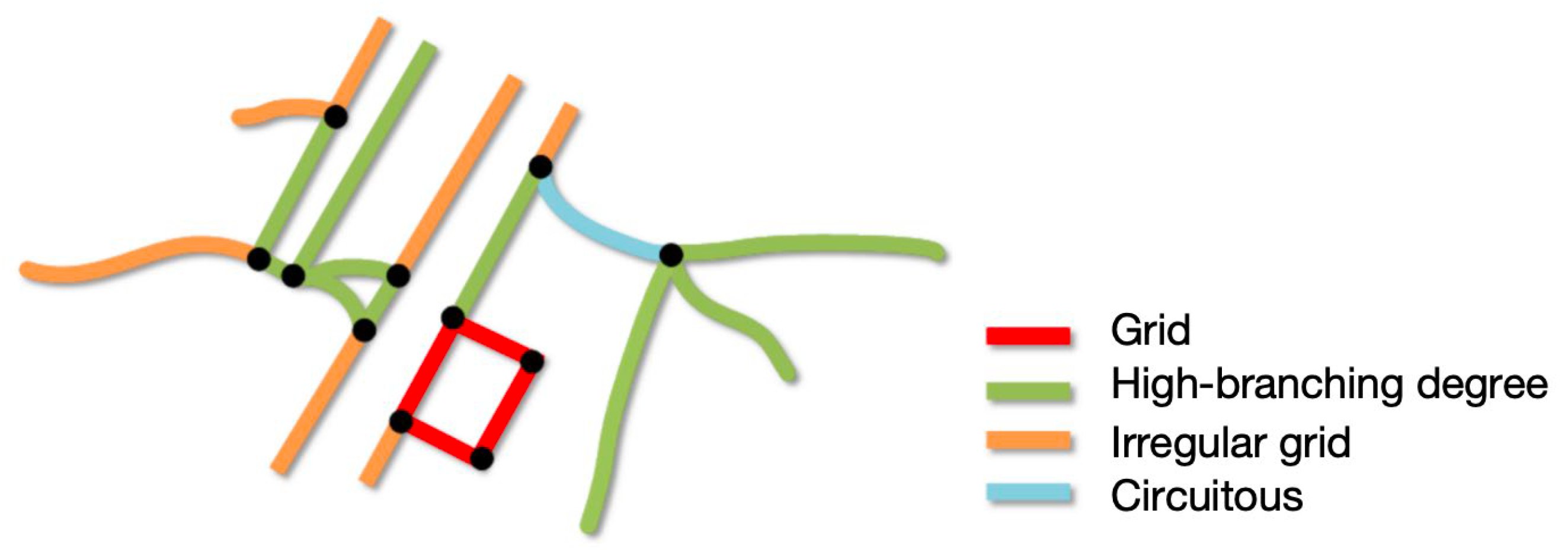
2.4.2. Spatial Patterns of the Road Network

Spatial pattern has been well studied in the road network literature, for various purposes. We follow the practice in Xue et al. [25], which uses an 11-dimensional feature vector and the K-Means clustering algorithm to classify spatial patterns in the road network. The feature vector consists of aforementioned features such as average node degree, node degree ratios, log circuity, bridge-edge–length ratio, bridge-edge ratio, end-edge–length ratio and end-edge ratio. As a result, four spatial patterns can be identified with this method (see Figure 3).

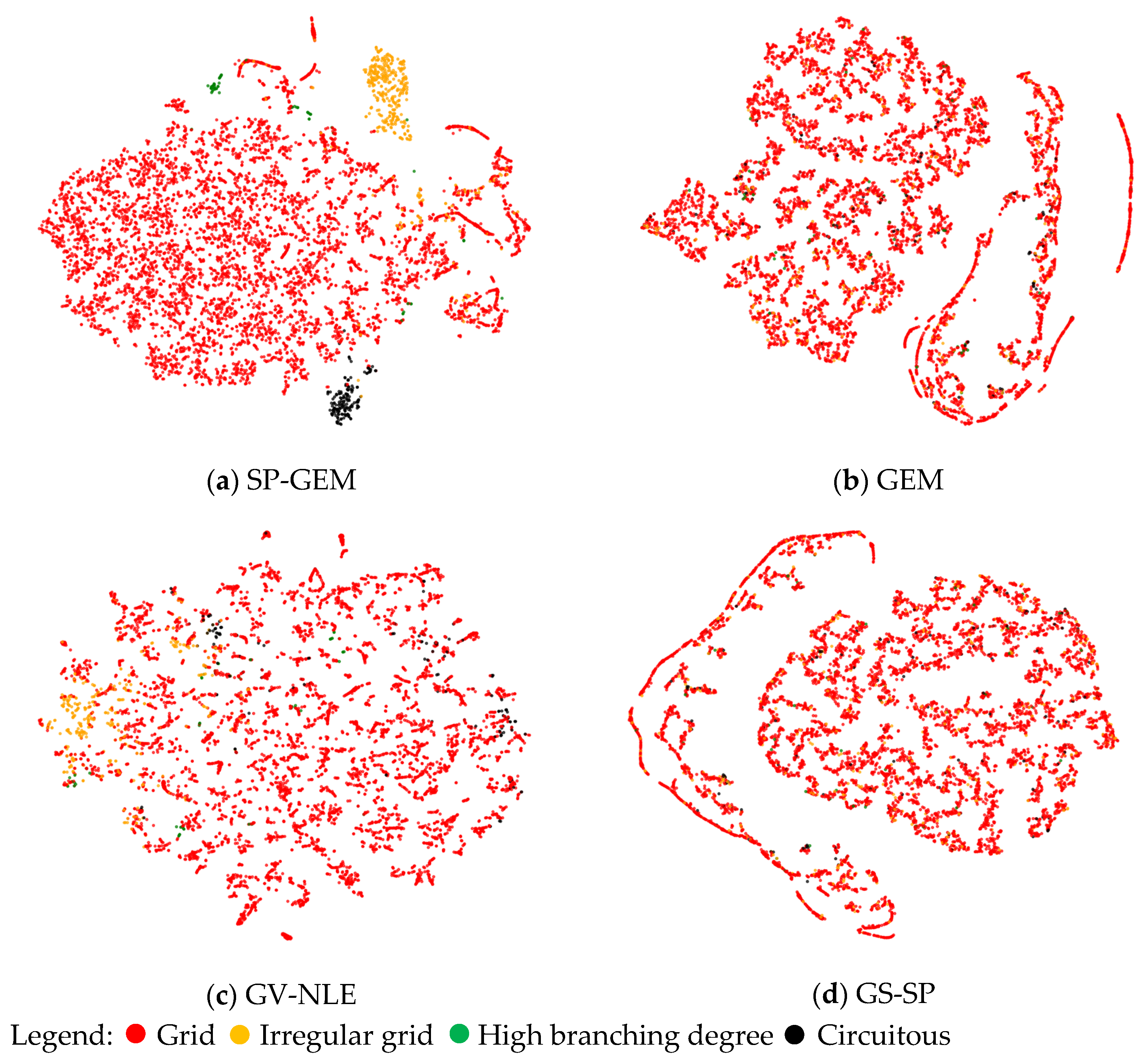
• Grid type has high average node degree, accompanied by low log circuity, bridge-edge ratio and end-edge ratio, reflecting a highly regular grid structure and homogeneous connectivity.
• High-branching degree type has the core feature that the proportion of nodes with node degree greater than or equal to 3 is significantly higher than that of other categories, and the average node degree reaches the maximum value, reflecting the complex multi-directional connection structure and high-density intersection attributes.
• Irregular grid type has a relatively high proportion of nodes with node degree of 1 and significant end-edge value, reflecting the existence of more termination points, incomplete connectivity areas in the network and the weak structural coherence.
• Circuitous type has significant high circuity value, bridge-edge ratio and end-edge ratio, showing obvious dependence on structural critical connectivity.

2.4.3. Spatial Pattern-Aware Neighbor Aggregation

Various efforts have been made with GNNs to leverage spatial patterns in road networks for computing node embeddings. Conventional GNN-based methods primarily capture the spatial attributes of neighboring nodes by incorporating spatial node features, but rely solely on node topology for neighbor aggregation. These approaches often lead to inadequate learning of the spatial relationships between nodes. Recent studies have shown a significant improvement in expressivity by introducing node distance into neighbor aggregation [24]. Inspired by the effectiveness of spatially explicit modeling, we propose a spatial pattern-aware neighbor aggregation function. The function explicitly models the spatial patterns of nodes’ neighbors, which consists of three main components, elaborated as follows.

(1)

Spatial division of node neighborhood. To capture the spatial patterns of a node’s neighborhood, we first establish a spatial orientation reference for the central node $v$. We divide the spatial neighborhood of the central node into eight orientation regions, $R=\{N,S,E,W,NE,NW,SE,SW\}$, where the base division of orientation $(N,S,E,W)$ is based on the four quadrants of the Cartesian coordinate system, with additional composite orientations ($NE$, etc.) determined by azimuthal intervals of ${45}^{\circ }$. This creates a subgraph partition that depicts the spatial distribution of the neighbor nodes. Next, we sample the neighbor nodes of the central node and calculate the Euclidean distance $|p_u-p_v|$ between each sampled neighbor node $u$ and the central node $v$, where $p_u$ and $p_v$ denote the coordinates of the two nodes, respectively.

(2)

Pattern-aware division aggregation. Considering that nodes with similar patterns in a road network often exhibit comparable spatial attributes and characteristics, we calculate the aggregated representation of neighboring divisions based on the spatial patterns of these neighboring nodes. For each division $r\in R$, the nodes that share the same spatial pattern $t\in T$ are summed up in terms of their features. The resulting sums are then normalized by dividing them by a normalization factor $c_v^{r,t}$, which represents the number of nodes sharing the same spatial pattern t within the neighbor division $r$ of the central node $v$. This normalization ensures that the aggregation process is not influenced by variations in the number of nodes, and balances the contributions of different patterned nodes within the same neighbor division. This approach helps prevent any single node from having too much or too little influence on the final node embedding.

(3)

Division-based neighbor aggregation. We weighted and summed the pattern embeddings of the eight divisions to obtain a comprehensive representation of the neighbor pattern of the central node. This neighbor representation integrates the spatial pattern features of different directions, providing a richer spatial pattern of the road network for updating the central node embedding.

Given that the pattern configurations differ among neighboring nodes, we establish learnable joint orientation–pattern weight matrices $W_{r,t}^k$ for each neighbor node embedding. This allows us to learn the node embeddings through a loss function $L\left(e_v\right)$. The weight matrix encodes the features of nodes that share the same neighbor partition and pattern. The loss function adaptively learns the embedding representation by ensuring that nodes with the same spatial pattern and neighbor partition remain close to each other in the embedding space. For the central node, we implement self-updating weights $W_v^k$ to preserve the topological information of the original node. This enables the central node to effectively combine features from various neighboring nodes, while retaining its core characteristics. The neighbor aggregation formula for the central node can be expressed as follows:

$$h_{\mathrm{v}}^{\mathrm{k}+1}=\sigma ({\sum }_{r\in R}{\sum }_{t\in T}{\sum }_{u\in N_{\mathrm{v}}^r(t)}{\displaystyle \frac{1}{c_{\mathrm{v}}^{r,t}}}{W}_{r,t}^k{h}_u^k\cdot |p_u-p_v|+W_v^k{h}_v^k)$$

(3)

where $\mathsf{\sigma }$ is the activation function, $N_v^r\left(t\right)$ is the set of neighbor nodes with spatial pattern $t$ in the neighbor division $r$ of the central node $v$, $h_v^k$ is the embedding vector of the node $v$ in layer $k$ and $h_u^k$ is the embedding vector of the node $u$ in layer $k$. The pseudocode for Algorithm 1 is shown below.

Algorithm 1: Spatial Pattern-aware Neighbor Aggregation

Input: $v$: center node u: neighbor node k: the number of layer $p_v$: coordinates of center node $p_u$: coordinates of neighbor nodes G: road graph $h_v^k$: embeding vector of the node $v$ at k-th layer $W_v^k$: center node’s weight at k-th layer $h_u^k$: embedding vector of the node $u$ at k-th layer $W_{r,t}^k$: orientation-pattern weight matrices of pattern $t$ in the r-th neighbor division $c_v^{r,t}$: normalization factor for of pattern $t$ in the r-th neighbor division of node $v$ Output: $h_v^{k+1}$: the node-embedding vector of center node at (k + 1)-th layer Initialize eight orientation regions R = {N,NE,E,SE,S,SW,W,NW} for orient_region r in R do   for neighbor_node u in G do     if u is not v then       current_orient_region = ComputOrientRegion($p_u$, $p_v$)       if current_orient_region == r then         euclidean_distance = sqrt($p_u$, $p_v$)         $h_v^{k+1}$ = $W_{r,t}^k$·$h_u^k$·euclidean_distance/$c_v^{r,t}$       end if     end if   end for end for $h_v^{k+1}$ = $h_v^{k+1}$ + $W_v^k$·$h_u^k$ $h_v^{k+1}$ = $\mathsf{\sigma }$($h_v^{k+1}$) end

2.5. Similarity Measure Using Road Embedding

After computing the embedding vectors of road segments in the given road network, we obtain vectors for each road segment and its neighboring features. During the matching process, we extract the node-embedding vectors for each stroke road segment from both the target and reference road networks, and stack the computed node-embedding vectors with the original geometric and topological features. We then calculate the Hausdorff distance between two road segments across the two networks. We employ three types of distances to assess the similarity between road embeddings: Hausdorff, Manhattan, and Cosine distance. Hausdorff distance measures the morphological differences between road segments, while Manhattan distance evaluates the positional differences between node embeddings. Cosine distance, on the other hand, gauges the directional similarity of road embeddings. By combining these distances, we comprehensively evaluate the similarity between roads within the target and reference road networks, generating a matching score for each pair of nodes through weighted summation. This score integrates both geometric and topological aspects of similarity, providing a comprehensive measure for road segment matching. The road segment-embedding similarity can be written as

$$\mathrm{S}\mathrm{c}\mathrm{o}\mathrm{r}\mathrm{e}(v,u)=W_{\mathrm{H}}\cdot \mathrm{D}\mathrm{i}\mathrm{s}{\mathrm{t}}_{\mathrm{H}}(v,u)+W_{\cos }\cdot {{\mathrm{D}\mathrm{i}\mathrm{s}\mathrm{t}}_{\mathrm{c}\mathrm{o}\mathrm{s}}}^{\prime }(v,u)+W_{\mathrm{M}}\cdot \mathrm{D}\mathrm{i}\mathrm{s}{\mathrm{t}}_{\mathrm{M}}(v,u)$$

(4)

$${{\mathrm{Dist}}_{\cos }}^{\prime }(v,u)=1-{\mathrm{Dist}}_{\cos }(v,u)$$

(5)

In Equation (4), the weights of the Hausdorff, Cosine, and Manhattan distances are represented by $W_H$, $W_{cos}$, and $W_M$, respectively. The term Dist_H$(v,u)$ represents the Hausdorff distance between road segments, while ${{Dist}_{cos}}^{\prime }(v,u)$ and ${\mathrm{D}\mathrm{i}\mathrm{s}\mathrm{t}}_{\mathrm{M}}(v,u)$ denote the Cosine and Manhattan distances between the road embeddings. The Cosine distance can be calculated using Equation (5), where ${Dist}_{cos}(v,u)$ represents the cosine similarity between road embeddings. If the embedded similarity of two nodes falls below the predefined matching threshold, the road segments corresponding to those two nodes are considered a matched pair; otherwise, they are not matched. The overall road-network matching task is implemented by comparing all road segment pairs.

3. Experiments and Analysis

3.1. Experimental Setup

3.1.1. Experimental Design

Two data sources, OpenStreetMap (https://www.openstreetmap.org/ (accessed on 11 July 2025)) (OSM) and Tele Atlas are used to conduct road-network matching experiments. OSM is a opensourced global map dataset, which contains basic geospatial feature data such as POI, street, river and building footprints. These data are contributed and updated by volunteer users worldwide, with a high degree of openness and flexibility. Tele Atlas is a commercial map provider which uses professional mapping vehicles for data collection. Using these data sources, we verify the algorithmic accuracy and analyse the quality of the embeddings of SP-GEM with the two experiments described as follows.

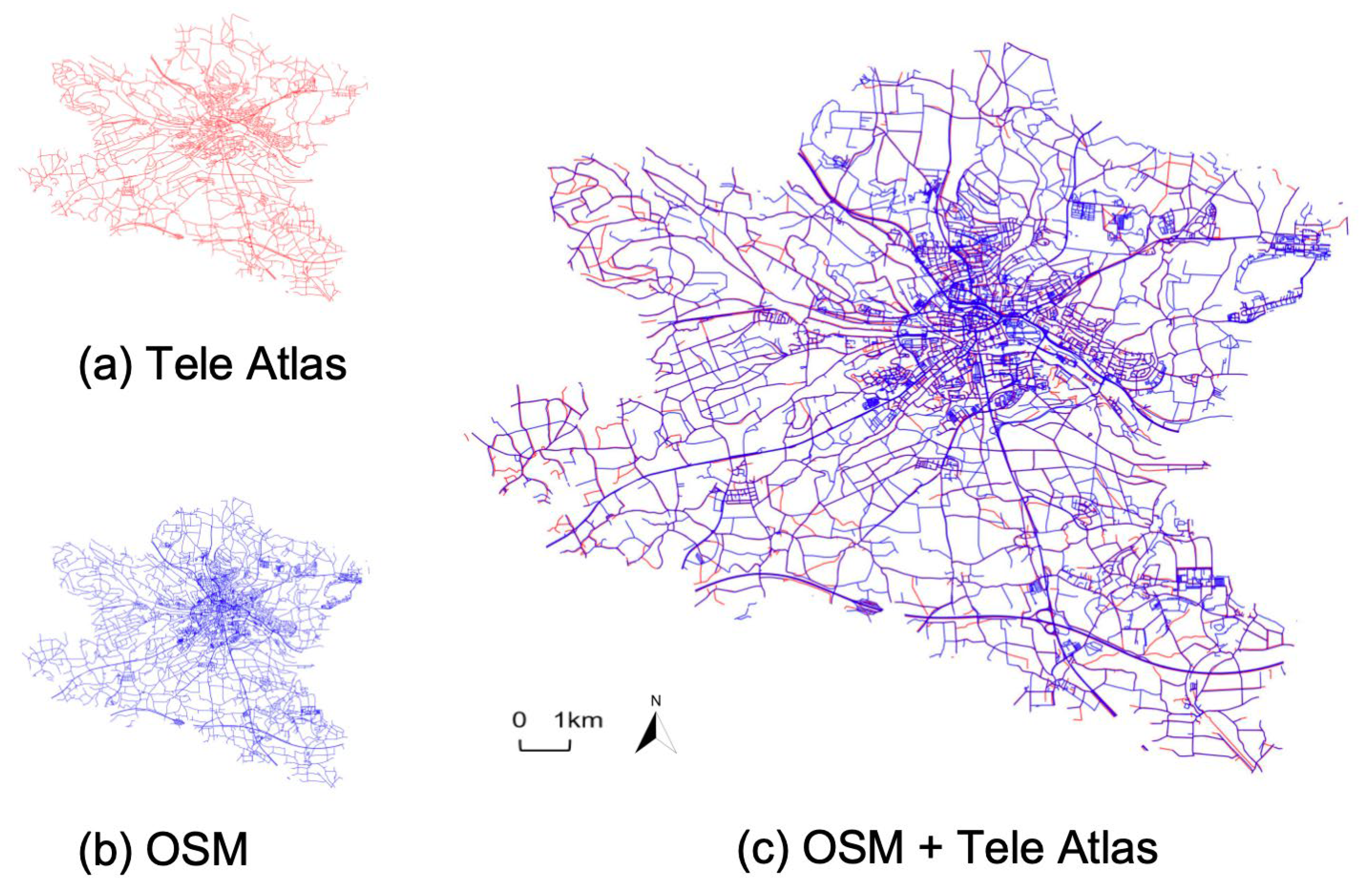
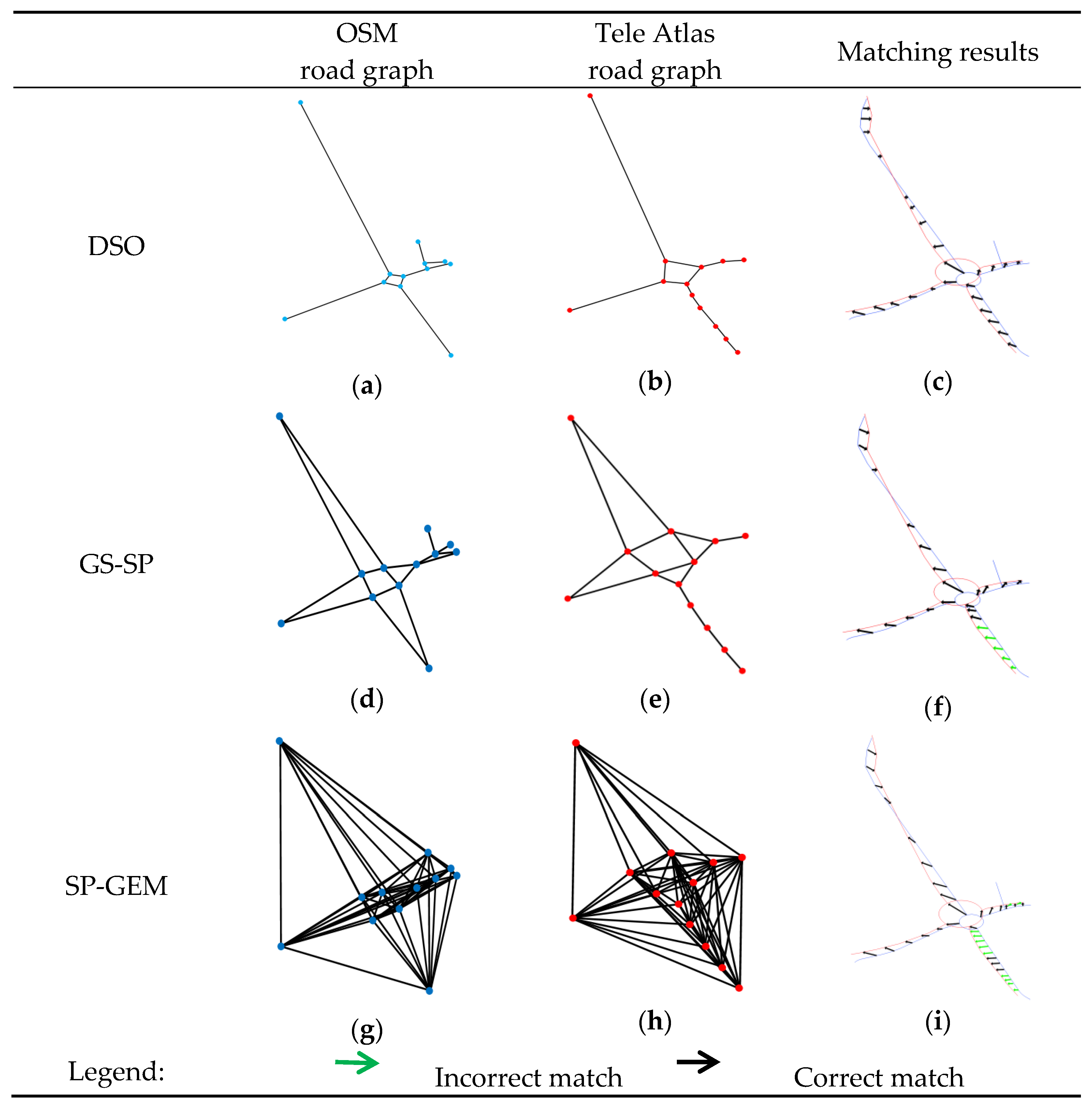
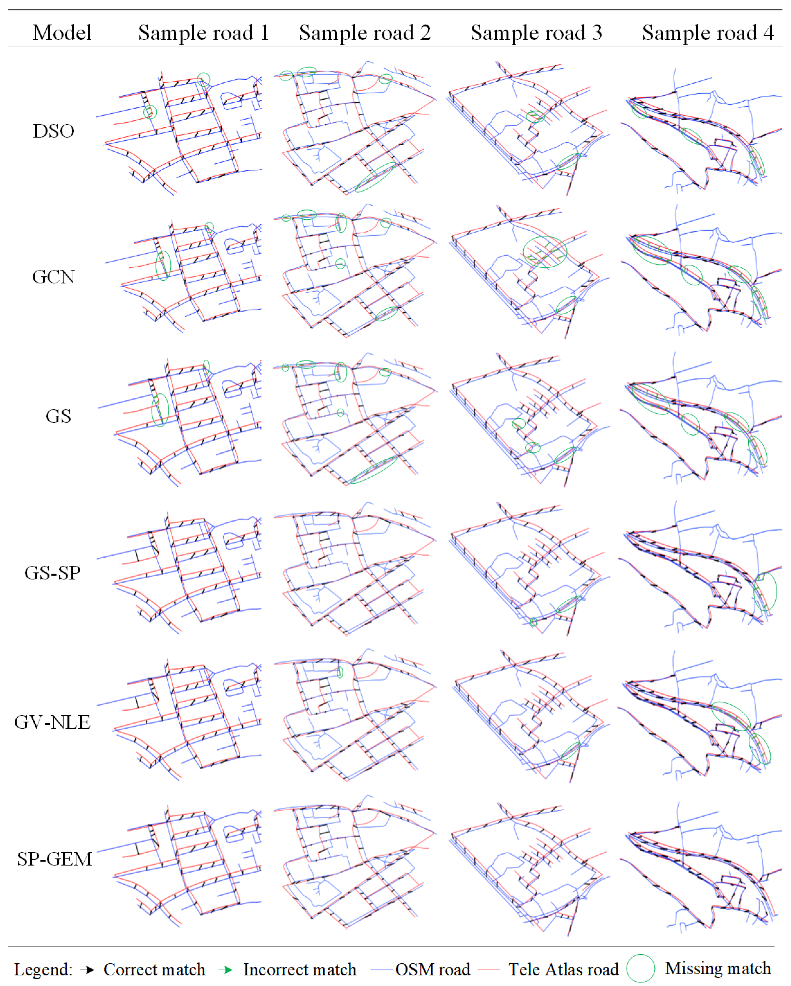
• The algorithmic accuracy experiment is used to compare SP-GEM with baseline algorithms using metrics of accuracy, recall and match rate. The experiments are conducted on road network data of the city Ansbach in Germany from both OSM and Tele Atlas, which reveal significant differences in road data modeling and acquisition time.
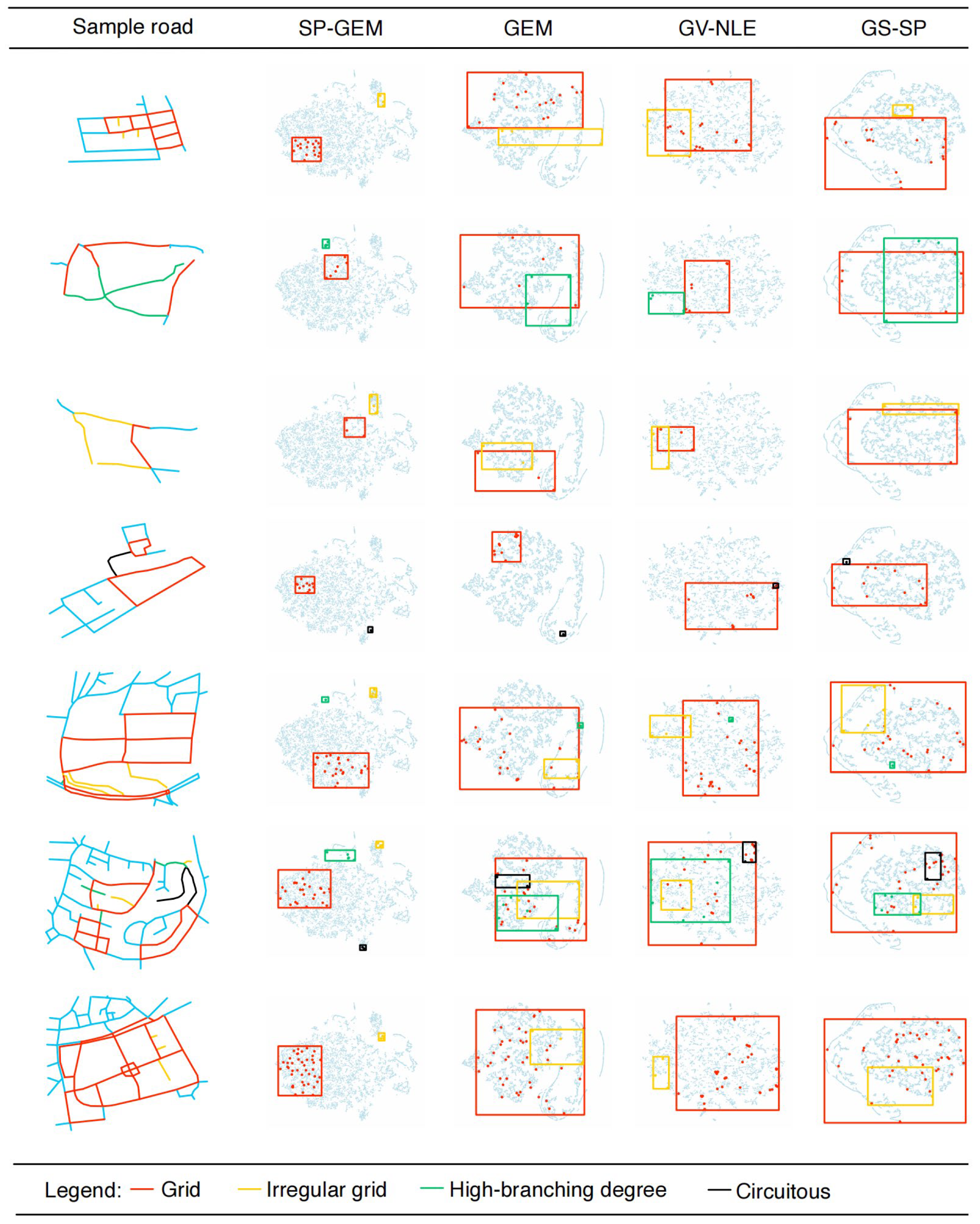
• The embedding analysis experiment evaluates the embedding performance of the algorithms in recognizing different road network patterns, as well as the effectiveness of integrating such capability into road neighbor modeling.

3.1.2. Evaluation Metrics

Three metrics are used to evaluate algorithmic performance, i.e., matching correctness (accuracy), recall, and matching success rate (match), which are written as

$$\mathit{accuracy}=1-(b/(a-c))$$

(6)

$$\mathit{recall}=(a-b-c)/d$$

(7)

$$\mathit{m}\mathit{a}\mathit{t}\mathit{c}\mathit{h}=(a-c)/a$$

(8)

where $a$ denotes the total number of road segments in the test area, $b$ denotes the number of incorrectly matched road segments, $c$ denotes the number of road segments that failed to match (i.e., no matching road segments could be found), and $d$ denotes the number of road segments that should actually be matched.

3.1.3. Implementation Details

We implemented the road graph construction and graph embedding algorithms using the machine learning framework Tensorflow, and the road-network matching experiments were carried out on a computer with a graphics processing unit of RTX 6000. In the road graph construction, the query threshold of graph node neighbor is set to 400 m. In the feature extraction, the LSTM batch size is set to 128, the sequence length to 256, the hidden layer size to 128 and the learning rate to 0.001. In graph embedding learning, the unsupervised learning method of GraphSAGE is used to generate training samples using the random walk algorithm for GNNs training. According to experimental results, GraphSAGE is selected with a hidden layer channel number of 256, a batch size of 512, a learning rate of 0.00001 and a random walk with a step size of 3 and a step count of 7.

3.2. Experimental Results and Analysis

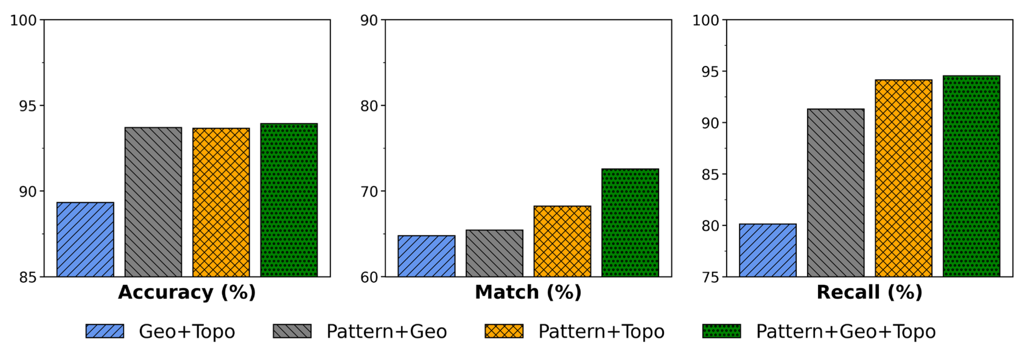
3.2.1. Experiment 1: Algorithmic Accuracy

The experiment uses road network data (see Figure 4) in Ansbach from OSM and Tele Atlas for algorithmic accuracy evaluation. After road-network stroke extraction, there are 12,785 OSM road segments and 7523 Tele Atlas road segments in the study area. And the manually labeled ground truth of the road-network matching between OSM and Tele Atlas is acquired from Yang et al. [24].

The baseline methods in the algorithmic accuracy experiment include DSO, GCN, GS, GS-SP, and GV-NLE. DSO [9] is a classical road-network matching algorithm, which achieves overall optimal matching by incorporating the topology and contextual information of the road network. GCN [20] is a conventional GNN-based method that captures the local structure of road segments through graph convolution and learns the global features of the road network through multilayer convolutional neural networks. GS [22] is a conventional GNN-based method proposed by Here (https://www.here.com, accessed on 11 July 2025), which uses the GraphSAGE framework to compute road embedding and achieve road-network matching with an embedding-based similarity measure. GS-SP [24] extends GS with a spatially explicit model design that computes node embedding based on the road center point’s spatial distance and road-type differences. GV-NLE [26] is a fastText-based embedding method used to transform OSM entities to embedding vectors for the downstream machine-learning task (https://geovectors.l3s.uni-hannover.de, accessed on 11 July 2025). Since we are interested in developing a GeoEmbedding service of road network data, it would be worthwhile to compare SP-GEM with such an embedding service. The implementation of the above-mentioned baselines follows the procedures defined in the literature.

The experimental results, as shown in

Table 3. Comparison of road-network matching performance in Ansbach using OSM and Tele Atlas data.

	DSO	GCN	GS	GS-SP	GV-NLE	SP-GEM
Accuracy	81.25%	76.21%	75.66%	87.27% *	93.14%	93.94%
Recall	82.60%	76.24%	77.51%	84.37% *	87.69%	94.54%
Match	73.87%	68.21%	69.31%	75.26%	57.97%	72.58% *

Note: The best, second-best, and third-best performances are denoted in bold, underlined, and with an asterisk *.

, show that although the SP-GEM performs excellently in terms of accuracy and recall, its match rate is lower than that of GS-SP and DSO, which are 2.68% and 1.29% lower, respectively. Specifically, SP-GEM improves the accuracy and recall rate by 6.67% and 10.17%, respectively, compared with the GS-SP, which adopts the spatially explicit modeling, demonstrating the model’s significant advantages in these two metrics. And when comparing it with the GCN, GS, and GV-NLE, which do not adopt such a modeling strategy, SP-GEM has the highest accuracy, which is improved by 3.27% compared to GS, while the accuracy and recall are improved by at least 0.8% and 6.85%, respectively.

As shown in Figure 5, although SP-GEM demonstrates advanced performance in terms of accuracy and recall metrics, it does not achieve optimal results for the match metric. To understand such insufficiency, we select a ring-road network for the case study. For the lower section of the ring-road network, the OSM road is represented by one segment, while the Tele Atlas road is represented by five connected segments, with significant differences in data structure.

The matching results show that the DSO is not affected by the inconsistent granularity of the segmentation of roads, because it utilizes the topology of the road segments and adopts the growth strategy for road-network matching. Since there is only one road segment connected to it in the same direction, according to the matching strategy, it will continue to match along the direction of the matching road segment, thus obtaining a higher match score.

The GS-SP and SP-GEM methods, on the other hand, both exhibit significant limitations in dealing with the case of inconsistent segmentation granularity. The GS-SP uses Hausdorff distance-based modeling to construct spatial-search graphs, and focuses on spatial geometric features in node neighbor modeling. In the sample ring-road network, the constructed graph model resembles a topological graph. As a result, in the lower section of the ring-road sections, the segments that are connected to the ring-road network can be matched correctly, but the rest of the road segments cannot be matched correctly, due to inconsistent node neighbor representations. This is due to varying segmentation granularity, and the graph model is different from the topological graph, which makes its match-success rates decrease, compared to DSO. When faced with one-to-many road segment correspondences, the node neighbor modeling of GS-SP struggles to establish accurate spatial-search graph correspondences, and this limitation directly affects the match metric.

As for SP-GEM, the spatial proximity graph models (e.g., Figure 5g,h) and their matching results (Figure 5i) demonstrate the node neighbor modeling based on spatial proximity. The differentiated matching results in the sections to the right and below the ring road being attributed to the spatial proximity followed by the method, i.e., the node context representation mainly relies on the role of the Euclidean distances between nodes in the graph construction. In particular, the matching relationship established in the middle road section exemplifies the matching capability of node neighbor modeling of spatial proximity graphs. However, due to the failure to form complete matches, as well as incorrect matches in some road segments, the match metrics are decreased compared with DSO and GS-SP. SP-GEM is able to identify some matches based on the spatial proximity context of nodes when dealing with the inconsistency of segment granularity, but there is still room for improvement in dealing with different segment granularity.

To assess the effectiveness of SP-GEM, we visualize and analyze the road-network matching results. As shown in Figure 6, sample road 1 and sample road 2 contain roads with different degrees of grid structure, and all methods except GS-SP and SP-GEM have matching errors. For sample road 3, there are more intersections in these road segments, and DSO, GCN, and GS also show more mis-matches. Sample road 4 consists mainly of highways, and is characterized by the presence of a large number of parallel road segments. In that case, only SP-GEM achieved zero matching error, while all baseline models failed to discriminate between the parallel roads in sample road 4, for their geometric similarity.

In summary, methods such as DSO, GCN, and GS are prone to mis-matching when dealing with complex road segments, especially when there are road segments within close proximity and similar structure, which can be easily misrecognized as matches. In contrast, SP-GEM has shown significant advantages in both matching accuracy and recall when facing complex road network structures. Compared with traditional road-network matching algorithms, SP-GEM improves the matching accuracy by exploring the spatial pattern for modeling road context, while mitigating the dependence of road-attribute data.

3.2.2. Experiment 2: Road Embedding Analysis

To understand the impact of incorporating spatial patterns into road embedding representations for road-network matching, we analyzed the road node-embedding structures of four models, i.e., SP-GEM, GEM (SP-GEM without the spatial pattern module), GV-NLE, and GS-SP. The analysis employs the t-SNE dimensionality reduction technique for embedding visualization.

We begin by visualizing the overall structure of road embeddings generated by different models and analyzing their clustering characteristics, as well as their ability to differentiate between various road network patterns. As illustrated in Figure 7, the embedding structure from SP-GEM demonstrates effective clustering of road patterns. In SP-GEM’s road embeddings, the central region forms a high-density cluster of grid-type road node embeddings, while the edge region contains a small number of irregular grid-type road nodes, circuitous-type road nodes, and high-branching-degree road nodes. This clustering structure indicates that the algorithm successfully learns pattern-aware node representations by integrating spatial pattern information. In contrast, the embedding structure from GEM is relatively loose, with significantly reduced aggregation of grid-type nodes. This suggests that the node embeddings produced by this algorithm, which lacks spatial-pattern constraints, are not effective in identifying patterns within the road network.

The embedding structure of GV-NLE falls in between the two; it maintains a degree of aggregation for grid-type road nodes, but has more dispersion compared to SP-GEM. Locally clustered irregular grid-type road nodes indicate that GV-NLE can capture some pattern-aware node representations. The successful representation of road nodes suggests that the algorithm partially captures road-pattern information, likely due to its strategy of using the FastText model for embedding road types and names. FastText excels at capturing word structures and semantic similarities of words. By integrating this semantic information with local topology, GV-NLE improves the clustering of functionally similar roads in the embedding space. However, circuitous and high-branching road nodes remain scattered, and are not effectively aggregated.

The embedding structure of GS-SP shows characteristics similar to the pattern-mixing distribution observed in GEM. However, this model incorporates one-hot encoding of road attributes, which only indicates categorical identification without capturing the semantic correlations or similarities between attributes. As a result, GS-SP struggles to effectively aggregate functionally or semantically similar road nodes in the embedding space, leading to a distribution pattern that resembles GEM, which underutilizes attribute information.

The comparison reveals that, when using the same model architecture, the effectiveness of the road network representation is significantly influenced by the spatial-pattern information of the model. This leads to notable differences in the embedding structures of the SP-GEM algorithms, resulting in varying capabilities for distinguishing road network patterns. Other models, such as GEM, GS-SP, and GV-NLE, also struggle with road network-pattern discrimination, due to their inability to implement effective spatially explicit modeling.

To better understand the role of spatial pattern in road neighborhood aggregation, we selected several sample roads that exhibit diverse road network-pattern structures. We examined the proximity of road neighborhood node embeddings using dimensionality reduction visualization techniques. As illustrated in Figure 8, four types of road network patterns were annotated for each sample road, along with their corresponding distribution ranges in the embedding space. By analyzing the proximity among roads that share the same pattern and assessing the overlap between different patterns, we can gain valuable insights into how spatial-pattern information influences road neighborhood modeling. The SP-GEM embeddings demonstrate a high level of proximity among roads of the same pattern, while clearly separating different pattern types. In contrast, the GEM method can distinguish pattern-specific roads in certain instances, but it generally shows mixed distributions across most samples. Further analysis of GV-NLE and GS-SP reveals that, being methods that do not explicitly incorporate spatial-pattern information, they tend to produce embeddings in which roads of the same pattern are scattered and roads of different patterns are heavily intermingled. In summary, integrating spatial-pattern information significantly enhances the model’s ability to capture contextual differences among roads, thereby improving the cohesion of similar road features and the distinguishability between different road types.

4. Discussion

We use feature ablation experiments to understand the effects of geometric features, topological features, and spatial pattern on the algorithmic performances. By sequentially removing geometric features, topological features, and spatial pattern information, we compared the matching accuracy, recall, and match rate of SP-GEM.

The results of the ablation experiments, as shown in Figure 9, indicate that the spatial pattern (referred to as “Pattern”) is crucial for improving the matching performance of SP-GEM, particularly in heterogeneous data with complex road network structures. In the Ansbach test area, the accuracy of the combination that includes Pattern exceeds 93%, which is significantly better than the accuracy of the Geo+Topo combination, at 89.33%. Furthermore, the match rate for the combination of Pattern, Geo, and Topo is 72.58%, representing an improvement of 7.79% compared to the Geo+Topo combination, which had a match rate of 64.79%. The combination of Pattern and Topo achieves a match rate of 68.24%, outperforming Pattern and Geo, which has a match rate of 65.44%. This highlights the central importance of Pattern and its effectiveness, when combined with topological features (Topo), in adapting to changes in the road network. Recall analysis further supports these findings, showing that the combination of Pattern, Geo, and Topo has the highest recall rate, at 94.54%. Additionally, the recall rate for Pattern and Topo is 94.14%, significantly surpassing the rate for Pattern and Geo, at 91.31%. In contrast, the Geo+Topo combination only achieves a recall rate of 80.13%, once again underscoring the essential role of spatial pattern information.

The analysis of the three metrics shows that the spatial pattern is the key model design in achieving better algorithmic performance, especially when dealing with data with temporal difference. Additionally, the spatial pattern enhances both the accuracy of matches and the overall success rate of matching. It works particularly well in combination with various types of features, demonstrating notable complementarity. In particular, when combined with Topo features, it proves to be especially effective in handling heterogeneous road network data sources collected over an extended time period. This finding provides a solid empirical basis for the road network matching strategy using multidimensional information fusion.

5. Conclusions

We propose SP-GEM, a spatial pattern-aware road network graph-embedding matching method, to achieve high algorithmic accuracy and robustness on real-world data. With spatially-explicit modeling, we explore the use of spatial patterns in computing road embedding, which improves the expressivity of the graph embedding representation of the road network. Extensive experiments are conducted on road network data from multiple sources and urban regions. The algorithmic accuracy experiment in Ansbach shows that SP-GEM improves the matching accuracy and recall by at least 6.7% and 10.2%, respectively, compared to the baseline method, with a high matching success rate (>70); it also improves the matching precision and recall by at least 17.7% and 17.0%, respectively, compared with the baseline graph neural network without spatially explicit modeling. This study further conducted a road network embedding analysis on the Ansbach dataset,t to examine how spatial pattern awareness affects road network matching performance across varying environmental road networks. This study not only provides an effective and practical algorithm for road network matching, but also serves as a test bed in exploring the role of spatially explicit modeling in GNN-based road network modeling.

Several improvements can be identified for SP-GEM to address issues such as the time-consuming model training, and the parameter selection for constructing spatial proximity graphs. For instance, the full Ansbach dataset required approximately 10 h to complete training on a single NVIDIA RTX A6000 GPU. Therefore, further exploration of efficient graph-learning algorithms (e.g., graph partitioning and sampling) could facilitate practical applications of SP-GEM. Moreover, this study only focus on city regions of European cities, which calls for a more comprehensive validation for worldwide applications, including underdeveloped cities. Additionally, developing a road network similarity assessment service based on GeoEmbedding (i.e., transforming geospatial data into vector representation) would be desirable, as it could provide machine learning-friendly data references for scientific discovery and policy-making, based on open-source road network data.

References

1. Wang, Y.; Yan, H.; Lu, X. Hierarchical semantic similarity metric model oriented to road network matching. J. Geo-Inf. Sci. 2023, 25, 714–725. [Google Scholar]
2. Yang, J.; Zhang, M.; Fang, L.; Jia, F.; Zhou, G.; Zhang, J.; Yang, M.; Hou, Y. Quality assessment of OpenStreetMap road network data using multisourced data matching and conflation. J. Geomat. Sci. Technol. 2024, 40, 526–533. [Google Scholar]
3. Sun, Q. Research on some fundamental issues of spatial data similarity. J. Geomat. Sci. Technol. 2013, 30, 439–442. [Google Scholar]
4. Sun, Q. Research on the progress of multi-sources geospatial vector data fusion. Acta Geod. Et Cartogr. Sin. 2017, 46, 1627–1636. [Google Scholar]
5. Wu, B.; Wang, Z.; Yang, F. A semantic similarity computational model for multi-scale road network matching. Sci. Surv. Mapp. 2022, 47, 166–173. [Google Scholar]
6. Tan, Y.; Tang, Y.; Li, X.; Liu, B.; Wei, X. Semantic-based geographic feature property similarity measurement model. Remote Sens. Inf. 2017, 32, 126–133. [Google Scholar]
7. Wang, H.; Zhai, R.; Zhou, M.; Zhu, L. A road matching method based on complex networks. J. Geomat. Sci. Technol. 2016, 33, 88–93. [Google Scholar]
8. Zhang, M.; Shi, W.; Meng, L. A generic matching algorithm for line networks of different resolutions. In Proceedings of the Workshop of ICA Commission on Generalization and Multiple Representation Computering Faculty of a Coruña University-Campus de Elviña, La Coruña, Spain, 7–8 July 2005. [Google Scholar]
9. Zhang, M.; Wang, Q.; Haizhong, Q. A generic algorithm for automatic road-network matching between different data sets. J. Geomat. Sci. Technol. 2018, 35, 82–86. [Google Scholar]
10. Almotairi, M.; Alsahfi, T.; Elmasri, R. Using local and global divergence measures to identify road similarity in different road network datasets. In Proceedings of the 11th ACM SIGSPATIAL International Workshop on Computational Transportation Science, Seattle, WA, USA, 6 November 2018. [Google Scholar]
11. Qin, Y.; Song, W.; Zhang, Z.; Sun, X. Matching method for road networks considering geometric features and topological continuity. Bull. Surv. Mapp. 2021, 8, 55–60. [Google Scholar]
12. Wanpeng, C.; Pinghu, C. An urban road network entity matching algorithm based on similarity metric. Mapp. Spat. Geogr. Inf. 2018, 41, 39–42+46. [Google Scholar]
13. Li, C.; Li, T.; Zhou, X.; Tang, H.; Zhang, X.; Hu, K. Urban Road Network Matching Model Based on Fuzzy Hierarchy Theory and Its Application. Earth Sci. 2024, 49, 3020–3028. [Google Scholar]
14. Hacar, M.; Gökgöz, T. A new, score-based multi-stage matching approach for road network conflation in different road patterns. ISPRS Int. J. Geo-Inf. 2019, 8, 81. [Google Scholar] [CrossRef]
15. Kong, X.; Yang, J. A scenario-based map-matching algorithm for complex urban road network. J. Intell. Transp. Syst. 2019, 23, 617–631. [Google Scholar] [CrossRef]
16. Lu, H.; Feng, L.; Boya, W.; Lei, T.; Zong, Z. A dynamic social robot detection method based on link prediction matching. J. Inf. Eng. Univ. 2024, 25, 285–291. [Google Scholar]
17. Qingjie, M.; Dongxu, Y.; Yang, L. Prediction of molecular properties by graph neural networks incorporating sequence and structural features. J. Hunan Coll. Arts Sci. (Nat. Sci. Ed.) 2024, 36, 12–18+56. [Google Scholar]
18. Wang, M.; Ai, T.; Yan, X.; Xiao, Y. Graph convolutional network model for recognizing road orthogonal grid patterns. J. Wuhan Univ. (Inf. Sci. Ed.) 2020, 45, 1960–1969. [Google Scholar]
19. Zhang, H.; Yang, J. Spatio-temporal generative adversarial clustering graph convolutional network for anomalous traffic flow prediction. Comput. Eng. 2025; in press. [Google Scholar]
20. Yu, H.; Ai, T.; Yang, M.; Huang, L.; Yuan, J. A recognition method for drainage patterns using a graph convolutional network. Int. J. Appl. Earth Obs. Geoinf. 2022, 107, 1–15. [Google Scholar] [CrossRef]
21. Yang, M.; Jiang, C.; Yan, X.; Ai, T.; Cao, M.; Chen, W. Detecting interchanges in road networks using a graph convolutional network approach. Int. J. Geogr. Inf. Sci. 2022, 36, 1119–1139. [Google Scholar] [CrossRef]
22. Soni, A.; Boddhu, S. Finding map feature correspondences in heterogeneous geospatial datasets. In Proceedings of the 1st ACM SIGSPATIAL International Workshop on Geospatial Knowledge Graphs, Seattle, WA, USA, 1 November 2022. [Google Scholar]
23. Gadi, H.K.; Liu, L.; Meng, L. Road Networks Matching Supercharged with Embeddings. In Proceedings of the 7th ACM SIGSPATIAL International Workshop on AI for Geographic Knowledge Discovery, Atlanta, GA, USA, 18 November 2024. [Google Scholar]
24. Yang, M.; Yang, J.; Hou, Y.; Lang, L.; Zhang, Z.; Zhang, B.; Zhang, J. A method of road network matching using graph embedding via improved neighbor aggregations. J. Geo-Form. Sci. 2024, 26, 2335–2351. [Google Scholar]
25. Xue, J.; Jiang, N.; Liang, S.; Pang, Q.; Yabe, T.; Ukkusuri, S.V.; Ma, J. Quantifying the spatial homogeneity of urban road networks via graph neural networks. Nat. Mach. Intell. 2022, 4, 246–257. [Google Scholar] [CrossRef]
26. Tempelmeier, N.; Simon, G.; Demidova, E. GeoVectors: A linked open corpus of OpenStreetMap Embeddings on world scale. In Proceedings of the 30th ACM International Conference on Information & Knowledge Management, Gold Coast, QLD, Australia, 1–5 November 2021. [Google Scholar]
Figure 1. SP-GEM’s overall framework. (a) Road graph construction, (b) road graph feature extraction, (c) spatial pattern-aware road embedding and (d) similarity measure based on road embedding.
Ijgi 14 00275 g001
Figure 2. Illustration of the variables of geometric features of road segments. Point O is the center coordinate, which is the arithmetic mean of the midpoints of all road segments, ( x 1 , y 1 ) are the coordinates of the midpoints of the road segments, d and b are the length and width of the MBR, and P1 and P2 are the two endpoints of the longest side of the MBR.
Ijgi 14 00275 g002
Figure 3. Spatial patterns in a sample road network.
Ijgi 14 00275 g003
Figure 4. Ansbach’s road network. Road data from (a) Tele Atlas, (b) OSM and (c) data overlay of the two sources.
Ijgi 14 00275 g004
Figure 5. Road graph modeling (a,b,d,e,g,h) and matching results (c,f,i) of a ring-road network.
Ijgi 14 00275 g005
Figure 6. Comparison of road-network matching results of sample roads.
Ijgi 14 00275 g006
Figure 7. Road embeddings of SP-GEM and baseline models, with highlights on road patterns.
Ijgi 14 00275 g007
Figure 8. Comparisons of road pattern-awareness in road neighbor modeling of SP-GEM and baseline models.
Ijgi 14 00275 g008
Figure 9. Ablation study of SP-GEM on test road network data from Ansbach.
Ijgi 14 00275 g009