An Innovative Proposal for Developing a Dynamic Urban Growth Model Through Adaptive Vector Cellular Automata

Abstract

Monitoring urban growth through simulation models is becoming increasingly vital for the sustainable management of cities. Although various raster-based models have been developed over the past three decades, the irregular, fragmented, and heterogeneous geometric structure of urban areas poses significant challenges to effectively modeling complex land use and land cover (LULC) transitions. To address these limitations, this study proposes a novel urban growth simulation model based on vector cellular automata (VCA). In this model, dynamic neighborhood relationships are flexibly established using an algorithm called growth vectors (GVs). Open-access data from four time periods between 1990 and 2018 were utilized for three major European metropolitan areas: Istanbul, Berlin, and Madrid. During the calibration phase, the model was trained using three machine learning algorithms: Random forest, support vector machine, and multi-layer perceptron. For the simulation phase, an adaptive VCA-based urban growth model was developed to predict LULC changes through to 2040. The results demonstrate that the proposed algorithm can achieve a satisfactory level of accuracy in modeling urban growth.

1. Introduction

Rapid and unbalanced urban growth has led to the consumption of natural resources, ecosystem degradation, inadequate urban infrastructure, and declining quality of life. In this context, monitoring land use and land cover (LULC) changes is crucial for investigating and developing strategies to mitigate the physical, environmental, and socio-economic impacts of urban growth. As cellular automata (CA) models for simulating urban growth are both geospatial and computationally efficient, they can effectively represent the complex characteristics of urban systems, such as self-organizing and self-similarity, and their spatiotemporal dynamic structure and non-linear behaviors [1,2,3]. Therefore, several models have been created using raster-based CA (R-CA) models to simulate urban growth.

Raster-based CA models, with their regular grid structure, often struggle to accurately capture complex land use transitions in urban environments due to their irregular and fragmented geometries [4]. In Vector Cellular Automata (VCA), cells are the fundamental units of urban development, planning, and land policy, with urban growth representing changes in land cover based on these cells [4]. Since each cell is unique, neighborhood factors and their effects can be defined more flexibly when constructing the transition rules.

Choosing the right cell size is another significant issue for R-CA, as a larger size reduces geospatial accuracy and data volume [5]. Vector data enables a more realistic and detailed representation of geographic features [6]. In the VCA algorithm, each object, such as LULC, is geometrically represented by polygons that are influenced by geographical neighborhood relationships. Changes in the states of these objects over time are determined by a transition function [7]. The geometry and attributes of geospatial objects can be inserted into the cells in the VCA model. In this way, the transition rules of the model can be derived considering the spatiotemporal dynamics of the LULC change [8]. Moreover, VCA’s capability to operate on a parcel basis allows for the creation of high-resolution models, enhancing model accuracy and facilitating more comprehensive socio-economic analysis [4,8,9].

The purpose of this study is to develop a new adaptive model based on VCA to monitor uncontrolled urban growth by establishing dynamic neighborhood relationships based on spatial proximity, geometric characteristics, and local factors. This is accomplished by developing an abstract computational surface known as a growth vector (GV). This approach aims to differentiate the land surface from the computational surface, enabling the development of a practical integrated model that facilitates transitions between the two. Additionally, new neighborhood and transformation rules are established using the GVs.

The model uses input data in vector format, primarily derived from the CORINE Land Cover (CLC) database of the European Union. Transportation data sourced from the open-access OpenStreetMap (OSM) website were utilized to assess accessibility. The Shuttle Radar Topography Mission (SRTM) data from the United States Geological Survey’s (USGS’s) EarthExplorer web service served as the digital elevation model (DEM) for evaluating topographic suitability.

During the model calibration phase, the GVs were trained using three different machine learning algorithms: Random forest (RF), multi-layer perceptron (MLP), and support vector machine (SVM). The model validation phase involved calculating F1 scores, receiver operating characteristic (ROC) curves, and area under the curve (AUC) values.

Three important European metropolitan cities—Istanbul, Berlin, and Madrid—were selected as case studies to evaluate the applicability of this model across different urban environments. The varying geospatial and demographic characteristics of the selected cities provided a robust basis for evaluating the model’s adaptability. The aim was to assess whether the model is applicable to a broad range of urban typologies rather than being limited to a specific city type. The differences among the selected cities offered a valuable opportunity to evaluate the model’s flexibility and generalizability. Consequently, nine hybrid urban growth models were created for the year 2040 to examine LULC changes, and the findings demonstrated that the model can have a wide range of applications and can be an effective tool in predicting urban growth trends in different cities.

The article is organized into six sections. Section 1 introduces the study’s purpose, methods, and data sources. Section 2 provides a literature review highlighting the benefits of using VCA-based models to monitor LULC changes. Section 3 outlines the general workflow of the developed model, detailing the methods applied to assess urbanization potential, as well as the processes for model validation and data handling. Section 4 presents the findings of the study, and is followed by Section 5, which includes a discussion of the results. The article concludes with a summary in Section 6.

2. Advantages of VCA Models for Monitoring LULC Changes

Simulation modeling is a widely used tool to examine the spatiotemporal dynamics of urban growth. A cellular automaton is often favored in urban growth monitoring studies due to its simplicity, intuitiveness, transparency, and flexibility [10,11,12]. A classical cellular automaton consists of cells, time, transformation rules, neighborhood relations, and grid network components [13], providing a regular structure that aligns well with raster data formats. However, when dealing with complex systems like urban growth, this classical approach has limitations and requires adaptation [6,7,11].

The VCA model extends the traditional CA approach by enabling irregular spatial representations and supporting complex cell states, including various types of land use such as urban areas. Unlike the R-CA model, where cells typically have binary states (e.g., urban or nonurban), VCA allows cells to assume multiple land-use states. This enhancement enables more detailed and realistic simulations in urban growth models. To address the limitations of R-CA, the VCA model defines cells as polygons that can represent geographical entities irregularly [8,14]. Additionally, the neighborhood relationships between cells are expanded to accommodate irregular spatial structures, with distances and effects considered using varying weights [4,6,9,15].

A key advantage of the VCA model is its capacity to represent irregular geospatial structures, such as land parcels or administrative boundaries. Unlike R-CA models, which are based on regular grid structures, VCA models utilize irregular units, such as cadastral parcels. This approach provides a representation that is more aligned with the large-scale maps used in urban planning, allowing for a more realistic modeling of the dynamics of the LULC over time. Moreover, these irregular spatial units improve the accuracy of land cover simulations and support more effective urban planning [16].

In contrast to fixed neighborhood relationships in the R-CA, the neighborhoods in the VCA adapt based on distance and cell states [6]. Consequently, neighborhood relationships and cell states in the VCA must be defined more flexibly [17]. This flexibility enhances the simulation of the spatiotemporal dynamics of LULC, making it more realistic. The adaptable structure of the VCA serves as a powerful modeling tool, allowing us to gain a deeper understanding of the complexities inherent in urban growth systems.

The initial VCA models used Voronoi polygons [18] and Delaunay triangulation [19]. However, these polygons were generated automatically and did not accurately represent the actual geographic entities. Subsequent studies focused on individual parcels at the planning scale demonstrated the effectiveness of VCA models. The first practical application of VCA was the Vector-based Geographic Cellular Automata (VecGCA) model, created in Quebec, Canada [7].

Since 2015, studies on urban growth modeling using the VCA approach have gained significant attention. A model called the Vector-based Beijing Urban Development Model (V-BUDEM) was developed in the Yanqing district of Beijing, China [15]. Another study in the Jiangsu region of China demonstrated that VCA is a practical and effective method for simulating urbanization processes [8]. Additionally, research conducted in Madrid, Spain, integrated graph theory into VCA based on parcel data. This study examined the operability of VCA through the created graph structure, focusing on the combined applicability of VCA and graph structures while also aiming to reduce computational time to a manageable level rather than solely capturing historical urban growth characteristics [6]. Examples of hybrid studies conducted in recent years include VCA and various machine learning (ML) algorithms, such as ensemble learning [20], artificial neural networks [21], random forests [4], and deep forest algorithms [9]. These methods are used for calibration and the discovery of transformation rules.

Several approaches have been applied for flexible neighborhood and transformation structuring in studies based on the VCA method. This study introduces the GV method to address the limitations of existing UGSMs, which often rely on empirically defined parameters that may overlook local spatial characteristics. To address this limitation, we analyze the edge lengths of GVs using a gamma distribution and identify the maximum possible distance value that influences urban growth in the study area. This allows the model to better adapt to local-scale urbanization processes and fills a gap in the literature by representing transformation processes more realistically and flexibly.

3. Materials and Methods

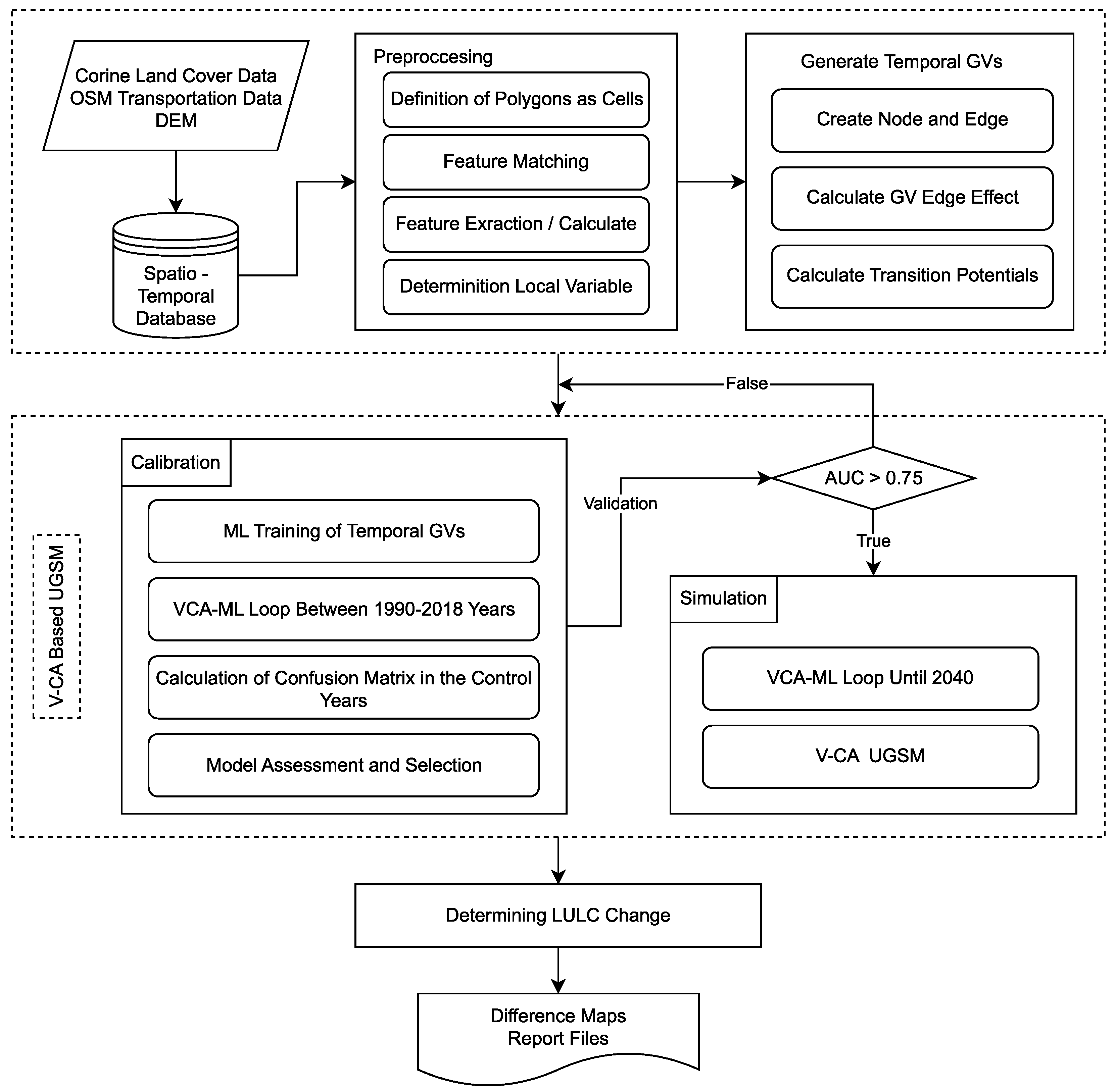
The VCA-based UGSM consists of three stages: preprocessing, calibration, and prediction (Figure 1). The preprocessing stage includes four sub-stages: defining the cells for the VCA, feature matching with other layers, feature extraction to determine unique cell attributes and derive data through spatial analysis, and defining local area parameters that influence the model’s behavior.

Polygons from the CLC data for 1990 and 2018 are treated as cells. In the feature-matching stage, these cells are connected with CORINE, OSM, and DEM layers, integrating their attributes. During feature extraction, geometric features like area and perimeter length are calculated, and an urban/rural classification is performed, resulting in a new layer attribute. Cell proximity to the road network is evaluated through buffer and overlay analyses applied to road-centerline data.

Slope values are extracted by overlaying DEM-derived raster slope data onto the vector cells. By conducting this analysis, a single slope value is calculated by averaging the slope values associated with each cell. Additionally, the urban/rural classification creates a separate layer attribute. The model defines two local variables: the critical slope, the highest slope value in urban areas; and the maximum urbanization distance. The maximum urbanization distance is determined by the model that uses temporal data specific to the study area. This model produces a value quantifying the effects of neighboring cells based on distance.

Once these processes are completed, GVs are created for the periods 1990–2000, 2000–2006, 2006–2012, and 2012–2018. A GV table is generated for each time interval, and all temporal GV tables are merged for use in model calibration. The GV created for each period represent the land cover class to which it belongs, as the dependent variable, within the corresponding time interval. The edge lengths of the GVs that contributed to urbanization in the previous periods are evaluated using a gamma distribution, which allows us to determine the highest possible singular distance value for the study area. Based on this value, we construct distance and corresponding probability matrices, ultimately deriving a global model through curve fitting, represented by a third-order polynomial equation. This equation provides the edge-effect values associated with the GV edge lengths throughout the model.

The temporal GVs generated reflect the amount of neighborhood interaction. The number of polygons directly determines the number of neighborhoods in the model for the years 1990, 2000, 2006, 2012, and 2018, as well as the areas of influence created by each polygon. This feature enables the model to analyze the relationships between neighborhood nodes, considering varying spatial and temporal conditions. Consequently, the model can assess whether urban growth will align with these relationships.

The calibration phase consists of two sub-stages: training and validation. In the training stage, GVs are trained using ML algorithms, including RF, SVM, and MLP. During the training and testing stages of the ML algorithms, the temporal GV dataset is divided into 70% for training and 30% for testing. This division is designed to maintain the distribution of the independent variable labels for urbanization and non-urbanization in both subsets. To achieve this, we use a stratified sampling method. This approach enhances the model’s generalization ability, particularly in datasets with imbalanced class distributions, allowing for a more reliable evaluation of the test data. Performance is evaluated using the F1 score. During validation, the simulated land cover data from the VCA-ML loop for 2018 is compared with the actual data using the ROC curve and calculating the AUC.

To evaluate the applicability of the proposed model in various study areas, we select three major European metropolises: Istanbul, Berlin, and Madrid. To examine the modeling capability across different LULC densities, we define the boundaries of the study areas based on specific land types rather than administrative districts. In Istanbul, the focus is on forested areas; in Berlin, we concentrate on residential neighborhoods; and in Madrid, we examine agricultural lands (

Table 1. LULC ratios of the study areas in 2018.

	Istanbul		Berlin		Madrid
	Rate	Area (ha)	Rate	Area (ha)	Rate	Area (ha)
Urban	11.04%	145,524.4	54.45%	88,515.4	8.07%	140,877.4
Agriculture	37.86%	499,278.3	25.85%	42,013.4	67.72%	1,181,387.5
Forest	51.10%	673,874.8	19.70%	32,020.1	24.21%	422,375.9
Total		1,318,677.5		162,579		1,744,641

).

In the simulation phase, the validated VCA-ML loop predicts land cover changes from 2018 to 2040, generating annual maps and change reports through LULC analysis. The process concludes with these yearly outputs.

3.1. Driving Factors (Spatial Variables)

Urban growth is influenced by various multidisciplinary factors, which can seem virtually limitless [2]. These factors include demographic, economic, environmental, political, technological, and social elements, allowing for some measurement and analysis [2,22,23]. This study uses a four-factor model—neighborhood, accessibility, suitability, and zoning—introduced by White et al. in 1997, which has become a standard in CA-based models [24].

The neighborhood factor not only identifies which cells are neighbors but also assesses the influence of the neighboring land cover classes by analyzing the interactions among land polygons [25,26,27]. However, the vector data structure exhibits varying neighborhood characteristics based on polygon size and land cover class due to irregularities in the structure [28]. In the model developed, neighboring polygons were determined using buffer zone analysis applied to each polygon. Thus, any polygons fully or partially within this buffer zone were classified as neighbors.

Neighboring-cell influence is modeled using a third-degree polynomial function based on inter-cell distances. This approach generates an edge-effect value based on the distance between cells in each generation, their land cover classes, and the Euclidean distance. The coefficients of the equation are determined through the curve-fitting method. As a result, the interactions among neighboring cells are modeled more realistically using a Gaussian distribution that accounts for distance [29].

When modeling LULC changes driven by urban growth using the CA method, the neighborhood relations between cells are crucial for defining the transformation rules. In a regular grid network, a growth model is based on the states of the neighboring cells of a selected cell. However, the irregular structure of the VCA model complicates the direct application of these neighborhood rules. Instead, the effect of the defined rule is determined by the model algorithm, which considers the region’s past growth trends.

In this paper, we define a rule $\left(R\right)$ based on the number of neighboring urban-type cells $\sum \left(N\right(x)$ surrounding a land part $\left(x\right)$ that has urban growth potential. This rule is included in the model as a parameter. The parameter is assigned a value of 1 if a cell has three or more urban neighbors, reflecting the trend toward urbanization (Equation (1)). Conversely, it takes a value of 0 if there are fewer than three urban neighbors [30]. Thus, while the model captures the tendency of urban areas to coalesce, it also restricts the expansion of low-density urban areas.

$$R{\left(x_i\right)}^{t+1}=\left\{\begin{array}{cc}\hfill 1,& \sum N\left(x_i\right)\ge 3\\ \hfill 0,& \sum N\left(x_i\right)<3\end{array}\right.$$

(1)

The suitability factor is another key component of the model, assessing the appropriateness of a land part for urbanization based on physical variables such as elevation and slope [30]. This model uses only the slope to evaluate suitability, utilizing SRTM data. A critical slope value of 20° was established, and the suitability of land areas with slopes below this was calculated using a linear gradient that increased as the value approached zero. The critical slope value can be tailored for local areas by analyzing existing urban cell slopes.

In Equation (2), with $0\le S$ and $0\le C\left(x_i\right)\le 1$,

$$C\left(x_i\right)=\left\{\begin{array}{cc}\hfill {\displaystyle \frac{CS-S}{CS}},& S\le CS\\ \hfill 0,& S>CS\end{array}\right.$$

(2)

The suitability values were normalized between 0 and 1, where S is the average slope, $CS$ is the critical slope value, and $C\left(x_i\right)$ is the suitability coefficient.

The other significant factor contributing to urban growth is accessibility [31]. The transportation data required for the model were sourced from the open-access OSM website [32]. In the model, the shortest distances to the road network were calculated by using a stepped buffer zone analysis, resulting in three levels of accessibility: areas within 500 m were classified as fully suitable, those between 500 and 1000 m were considered semi-suitable, and areas farther than 1000 m were deemed to have low suitability [33,34]. These distance ranges can be customized based on user inputs, allowing the determination of an accessibility coefficient for each land part. In Equation (3), d represents the shortest distance from a cell to the road network:

$$A\left(x_i\right)=\left\{\begin{array}{cc}\hfill \mathit{Fully}\mathit{suitable},& d\le 500\\ \hfill \mathit{Semi}-\mathit{suitable},& 500<d\le 1000\\ \hfill \mathit{Low}\mathit{suitability},& d>1000\end{array}\right.$$

(3)

The zoning parameter $\left(Z\left(x_i\right)\right)$ refers to legal attributes and indicates the legal status of cells in the model within the context of real estate law and planning (Equation (4)). This status helps determine the conformity of a polygon by considering its rights and restrictions in existing plans and regulations. As a result, the model can more accurately assess how legal and regulatory factors influence the suitability of cells for urbanization. It is important to note that planning data from the test regions were not included in this study. The analysis generated suitability predictions for urbanization in various land cover classes, excluding water bodies.

$$Z\left(x_i\right)=\left\{\begin{array}{cc}\hfill 0,& \mathrm{if}LC\left(x_i\right)\in \left\{\mathrm{Waterbody}\right\}\\ \hfill 1,& \mathrm{if}LC\left(x_i\right)\in \{\mathrm{Forest},\mathrm{Agriculture},\mathrm{Wetland}\}\end{array}\right.$$

(4)

In Equation (4), 0 represents a constraint, while 1 signifies a prediction suitable for urbanization. The zoning parameter can be classified according to various land cover categories, ranging from 0 to 1.

As a result, the transformation potential of each cell is as follows (Equation (5)):

$$P(x_i,t+1)=f\left(S(x_i,t),\sum _{x_j\in N\left(x_i\right)}{w}_{j}S(x_j,t),C\left(x_i\right),A\left(x_i\right),Z\left(x_i\right)\right)$$

(5)

In Equation (5), the cell state $x_i$ at time t is represented by $S(x_i,t)$, the weighted sum of neighboring cell states $({\sum }_{x_j\in N\left(x_i\right)}{w}_{j}S(x_j,t),C\left(x_i\right),A\left(x_i\right),Z\left(x_i\right))$, the suitability factor $C\left(x_i\right)$, the zoning factor $Z\left(x_i\right)$, and the accessibility factor $A\left(x_i\right)$. The state function $\left(f\right)$ calculates the transformation potential of the cell states at time t+1 through the interaction of factors.

3.2. Growth Vectors

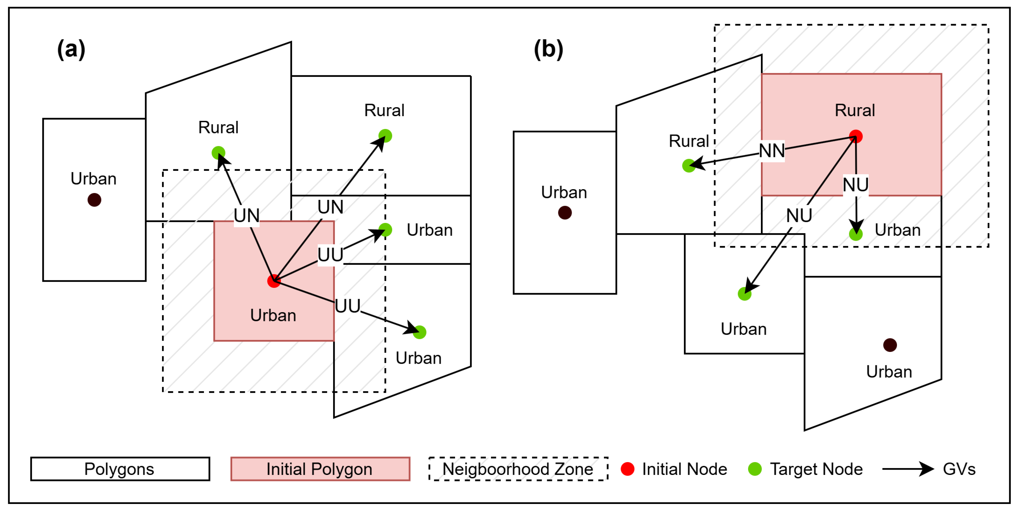
GVs are mathematical tools that simulate urban growth and represent vector data in a two-dimensional space. GVs are formed by converting polygons, called cells, into a point-node structure. Each node holds its own attributes, and edges are created between neighboring nodes, resulting in a network structure. These edges carry attribute information from the connected nodes and the calculated edge-effect value.

Figure 2 presents a schematic representation of the process by which GVs are generated. The developed neighborhood function sequentially selects each cell and applies a buffer analysis to its edges. An intersection analysis is then performed using the resulting buffer area. This approach enables the identification of neighboring cells not only based on shared edges but also on spatial proximity, allowing for the inclusion of nearby but non-adjacent cells as neighbors.

In Figure 2a, a node with the urban (U) attribute is positioned as the initial node, whereas in Figure 2b, the same node appears as a target node. Each generated GV, along with its associated attributes, is recorded in a separate layer to be used for training the ML algorithm.

Nodes are defined as centroids of polygons; however, if a centroid does not intersect with the surface of its corresponding polygon, a representative point is assigned on the polygon’s surface. For each selected polygon (initial), separate GVs are generated between its node and the nodes of all neighboring polygons (target). The direction of these vectors is defined from the initial node toward the target node.

A GV consists of two nodes and one edge, with directions based on their land cover type. If an urban (U) node connects to a rural (N) node, it is labeled UN (Figure 2). The model uses four labels: NU, UN, NN, and UU. The algorithm creates all GVs during the growth cycle and filters them by urbanization rules, focusing on those labeled UN. The urbanization potential of a GV is calculated by multiplying the potential of both nodes and an impact value based on the edge length (Equation (6)).

$$P_i^t={\left(PE\right)}_i^t\times K_i^t\times RD$$

(6)

In Equation (6), $P_i^t$ represents the urbanization potential of the selected node at time t. ${\left(PE\right)}_i^t$ indicates the transformation probability of the cell based on effective parameters, while $K_i^t$ refers to the transformation probability of the selected cell i influenced by neighborhood interactions. $RD$ represents the effective stochastic factors that cannot be accounted for [35].

An edge-effect value is generated based on the edge length formed between two neighboring cells. This value also determines the urban growth probability ($E_{ij}$) for the edge. The scores of the nodes for the edge ($P_i$), ($P_j$) and the edge $\left(E_{ij}\right)$ are multiplied to calculate the resulting transformation score $\left(P_{ij}\right)$ (Equation (7)).

$$P_{ij}=P_i\times P_j\times E_{ij}$$

(7)

A gamma distribution is used to determine the maximum singular distance of GV edge-length data attributed to urbanization. This distribution, defined by the shape $\left(\alpha \right)$ and scale $\left(\beta \right)$ parameters [36], is suitable for continuous positive data. In the study we first tested the distribution of the GV edge length and then estimated the highest effective urbanization length using temporal data from the local area.

The Kolmogorov–Smirnov (KS) test was used to assess the conformity of GV edge lengths to the gamma distribution [37,38]. This test calculates the largest absolute difference between the cumulative distribution of observed lengths and the theoretical gamma distribution, known as the KS statistic. A p-value greater than 0.05 indicates that the data fits the gamma distribution [39,40].

The maximum distance value ($d_{\max }$) for the study areas is determined by a specific point in the distribution, outlined in Equation (8), where the localization parameter “loc” represents the positive origin. This optimum distance point is found on the right side of the distribution, indicating a value greater than the mean and distanced from outliers.

$$d_{\max }=\mathrm{loc}+\alpha \times \beta$$

(8)

3.3. Model Calibration and Simulation Processes

The calibration phase is crucial for understanding changes in LULC. The combined use of the VCA and ML algorithms has recently become significant [4,41] in determining the binary state of a piece of land (urban/nonurban). During the model calibration process, modeled urban growth data are compared with actual data using the MLP, RF, and SVM algorithms. Only models with an AUC greater than 0.75 are used in the simulation phase.

The MLP algorithm is an artificial neural network capable of learning complex functions through non-linear activation functions [42,43]. It optimizes weights and enhances generalization performance by backpropagating error signals. Due to its self-organizing and adaptive properties, MLP has become a valuable tool in urban modeling studies [44,45,46,47,48]. The MLP consists of input, hidden, and output layers. Each hidden layer computes a new output using the outputs and weights of the previous layer.

The RF algorithm is often favored for modeling urban growth and LULC changes due to its ability to handle complex datasets and examine the relationships between various parameters [49,50,51,52,53]. It is a robust ensemble method among supervised learning algorithms [54].

In the second step, the RF algorithm, each decision tree is trained with data subsets created by the bootstrap method. At each node of the trees, branching is performed by identifying the attribute that provides the best split among randomly selected attributes. Thus, each decision tree performs a binary classification of urban and nonurban areas based on the attributes of the spatial variables in the input vector. The prediction from each tree is treated as a vote, and the final prediction is based on the majority vote from all the trees.

The third and final ML algorithm used to calibrate the model is the SVM. Its primary goal is to identify the hyperplane that maximizes the separation between different classes [55]. Since the SVM algorithm determines the classification results based on these separation boundaries, it cannot directly calculate the probability values [56]. However, the method, developed by Platt in 1999, has become widely adopted to make probabilistic estimates in SVMs [57].

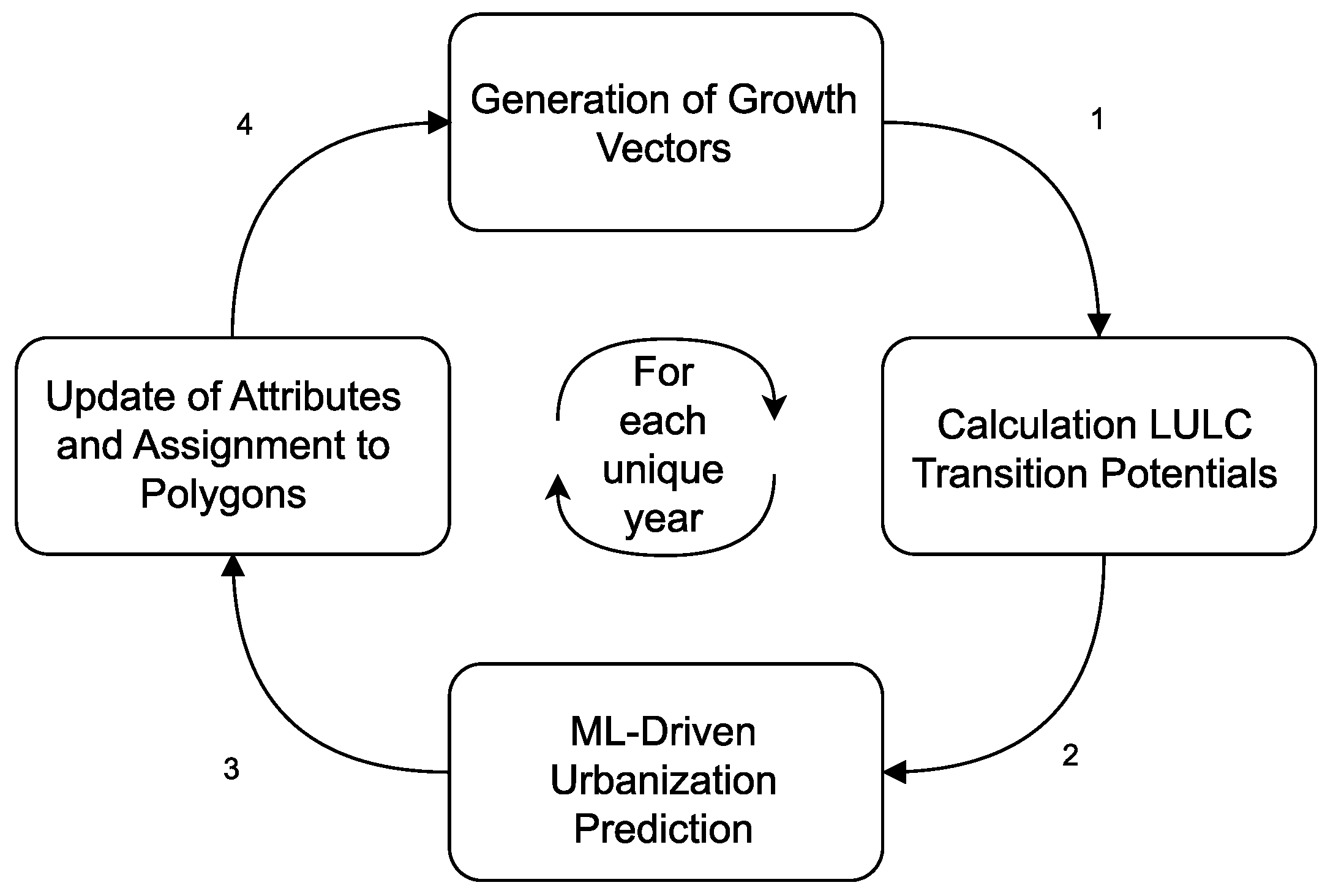
The three ML algorithms are trained using temporal GVs and integrated with the VCA. This iterative computational process, known as the VCA-ML loop, is a crucial step in both the calibration and prediction phases of the model. For each unique year in the model, a loop is created equal to the difference between the end and start years. The total number of loops corresponds to the number of iterations in the model, and each iteration consists of four successive steps (Figure 3).

In the second stage of the loop, which begins with the creation of GVs based on the actual LULC, the transition score is calculated for each GV. Following this, the decision phase starts, during which cells earmarked for urbanization in the upcoming year are identified. The restriction status of the target cell for the selected GV is first examined. If the cell is unconstrained, the transition score is calculated. If it is not zero, it is then compared to a randomly generated value from the model. If the transition score is greater than the random value, the urbanization potential of the GV is assessed using the ML model developed throughout the calibration phase. According to the results of this estimation, probabilities greater than 0.5 are classified as urbanization.

The growth vectors that generate urbanization define the LULC class of the target node as an urban area in the next generation. The nodes are then compared with the attributes of the polygon to which they belong. They are updated and prepared as input for the next iteration if a change is detected.

After the calibration step, the validation process begins to select the model for the simulation step. The study uses a two-stage validation process. First, the performance of the ML algorithms is evaluated with the F1 score. Next, the predicted land cover data for 2018 from the VCA-based UGSM are compared to the actual data, with ROC curves plotted to assess accuracy through the AUC values. A threshold of 0.75 is set for both the F1 score and AUC to ensure acceptable accuracy.

4. Results

Temporal land cover data for three distinct study areas were utilized to generate GVs for model training.

Table 2. GV counts of study areas between 1990 and 2018.

Study Area	Urban Growth	1990–2018				Timing Cost
		NN	NU	UN	UU
Istanbul	83%	9464	531	5675	2202	5’26.68”
Berlin	10%	11,354	200	7841	2240	3’36.60”
Madrid	110%	28,367	642	9481	3341	20’26.60”

presents the urban growth rates from 1990 to 2018 and the corresponding GV counts across four time intervals—1990–2000, 2000–2006, 2006–2012, and 2012–2018—for Istanbul, Berlin, and Madrid. The total number of GVs produced in the four periods was 17,872 in Istanbul, 21,635 in Berlin, and 41,831 in Madrid. LULC change rates were calculated for GVs labeled as ’UN’ (urban-to-nonurban interactions) across the four periods. The analysis indicates that connectivity between neighboring polygons begins at the “urban” nodes and terminates at “rural” nodes. The urban growth rates are as follows: 83% in Istanbul, 10% in Berlin, and 110% in Madrid.

The computation time for the model was measured based on the single-core performance of the CPU, taking into account the number of nodes, vertices, and edges in the polygons of the study areas. The recorded computation times were 5 min for Istanbul, 3 min for Berlin, and 20 min for Madrid. All calculations were conducted on a workstation equipped with an AMD Ryzen 9 9900X processor (12 cores, 24 threads, 5.6 GHz, 64 MB L3 cache) and 64 GB of RAM. The preprocessing and generation of the temporal GV stages, which incur the highest timing cost in the model, were completed in acceptable times.

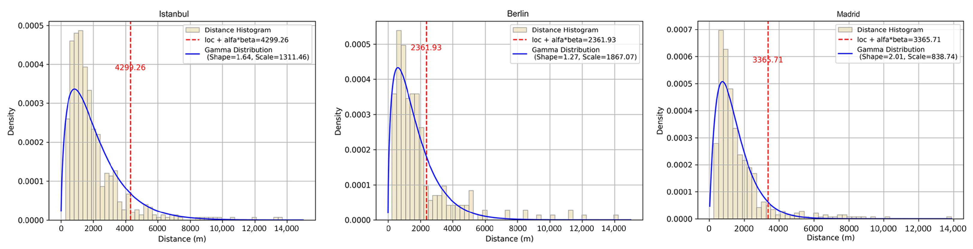
The fit between the (observed) continuous distribution of temporal GV edge lengths that generate LULC variation and the reference gamma distribution was examined to determine the maximum effect value “dmax” of the GV edge length (Figure 4). The KS test results statistically evaluated the conformity of the edge lengths to the gamma distribution in each study area. The obtained results for Istanbul were 0.0026 with a p-value of 0.88. In Berlin, these values were 0.0227 and 0.84, respectively. For Madrid, the KS statistic was 0.0102, and the p-value was 0.87.

The results show that the p-values are significantly above the 0.05 threshold for significance. This suggests that the edge lengths do not significantly deviate from a gamma distribution, indicating that this distribution is a suitable fit for the data in all three cities.

In practical terms, these findings support using the gamma distribution to describe the distribution of edge lengths in the VCA model. Specifically, an approach utilizing the gamma distribution parameters has been adopted for constructing distance-based probability matrices within the model’s transformation rules. This allows for a statistical representation of the heterogeneity of spatial structures, such as LULC cells and polygons, along with their geometric properties like edge length, shape, and orientation.

Consequently, the geometric diversity arising from spatial units (polygons) of various sizes and shapes can be numerically described using the gamma distribution. This enables statistical expression of structural differences within the model, ultimately enhancing both the realism and accuracy of the model.

As a result of this analysis, the dmax scores for each study area were 4299.26 m for Istanbul, 2361.93 m for Berlin, and 3365.71 m for Madrid (Figure 4). These values demonstrate the model’s ability to adapt to different spatial resolutions, as the dmax values are directly related to the surface area of the land cell compositions.

Although a direct correlation between the number of GVs and the LULC transformations cannot be established, the geographical distribution of these GVs in the study areas is significant for detecting such transformations. In the proposed model, GV density is both an indicator and a driver of urban expansion. Areas with a higher density of GVs typically represent regions where a greater number of temporal transitions (especially UN-labeled GVs) have occurred, signaling active land-use conversion processes. This density is not randomly distributed but is spatially aligned with known patterns of urban growth, such as expansion corridors, fringe developments, and infill zones.

Specifically, the locations where GVs are dense or rare can provide valuable insights. To illustrate this, the spatial densities of temporal UN-labeled GVs for four different time intervals from 1990 to 2018 are depicted in Figure 5. The data reveal GV concentrations in the northern forests and east–west corridors of Istanbul, northeastern and southern areas of Berlin, and the eastern and southwestern parts of Madrid.

During the calibration phase of the VCA-based UGSM, temporal GVs for four different periods spanning 28 years were analyzed using the RF, SVM, and MLP algorithms. The ML models developed for the study areas were then compared with a test set consisting of the temporal GVs divided by the stratified sampling method, and performance metrics were calculated (

Table 3. Performance metrics and parameter impacts of RF, SVM, and MLP for each city.

	Istanbul			Berlin			Madrid
Metric	RF	SVM	MLP	RF	SVM	MLP	RF	SVM	MLP
Accuracy	0.9380	0.9336	0.9258	0.9795	0.9734	0.9730	0.9770	0.9620	0.9757
Precision	0.9496	0.9484	0.9005	0.9885	0.9863	0.9878	0.9649	0.9630	0.9521
Recall	0.7267	0.7113	0.7127	0.8464	0.7985	0.7948	0.8244	0.6887	0.8244
F1 Score	0.8234	0.8129	0.7956	0.9119	0.8825	0.8967	0.8891	0.8031	0.8837
AUC	0.8586	0.8505	0.8463	0.9225	0.8984	0.8967	0.9103	0.8427	0.9096
Parameter
GV Direction	0.584	0.662	0.370	0.838	0.398	0.4397	0.613	0.535	0.343
GV Target Cell Area	0.110	0.020	0.153	0.057	0.128	0.0368	0.084	0.007	0.051
GV Initial Cell Area	0.070	0.310	0.208	0.037	0.082	0.117	0.050	0.396	0.161
GV Edge Effect	0.050	0.006	0.043	0.014	0.034	0.0586	0.043	0.001	0.079
Spatial Variables	0.186	0.002	0.226	0.054	0.358	0.3479	0.210	0.061	0.366

Note: Metrics represent model performance; parameters show relative importance in prediction skill.

). Model performance was assessed primarily using the F1 score, which balances precision and recall. While both the F1 and AUC scores demonstrated satisfactory accuracy levels for the ML algorithms, the relatively lower recall values—compared to other metrics—can be explained by the coarse spatial resolution of the input data, specifically the CORINE Level-1 dataset.

The RF algorithm demonstrated the best classification performance on the training dataset, achieving the highest accuracy and F1 score across all cities. Although the SVM algorithm performed worse than RF, the MLP model showed competitive results, reaching an F1 score close to that of RF in Madrid. All algorithms met the requirement of an F1 score greater than 75% to qualify for the validation phase.

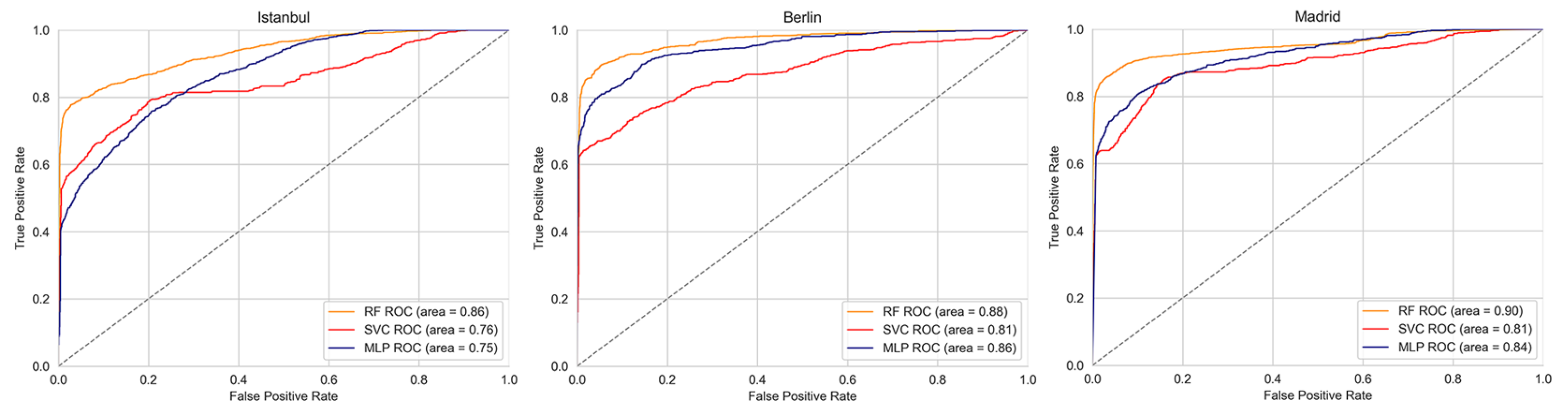
ROC curves were plotted during the validation phase, and the AUC statistics were calculated for all three VCA-ML models (Figure 6). The VCA-RF algorithm outperformed the others in all study areas, achieving the highest AUC values. Specifically, it scored 0.90 in Madrid, 0.88 in Berlin, and 0.86 in Istanbul. In Berlin, the VCA-MLP model performed comparably to the VCA-RF model, achieving an AUC value of 0.86, but it resulted in lower scores of 0.75 in Istanbul and 0.84 in Madrid. Meanwhile, the VCA-SVM model had relatively poor performance across all areas, with AUC values of 0.78 in Istanbul, 0.87 in Berlin, and 0.81 in Madrid.

The importance percentages of GV parameters for the ML algorithms utilized in the three cities—Istanbul, Berlin, and Madrid—are presented in Table 3. The results indicate that while the GV parameters, such as direction, target cell area, initial cell area, and edge effect, varied across different cities and models, GV direction emerged as one of the most influential factors in all locations. In order, the parameters with the most significant impact on GV are direction, initial cell area, target cell area, and edge effect. As illustrated in Table 3, GV direction has the highest impact level in this study, which models urban growth across various study areas.

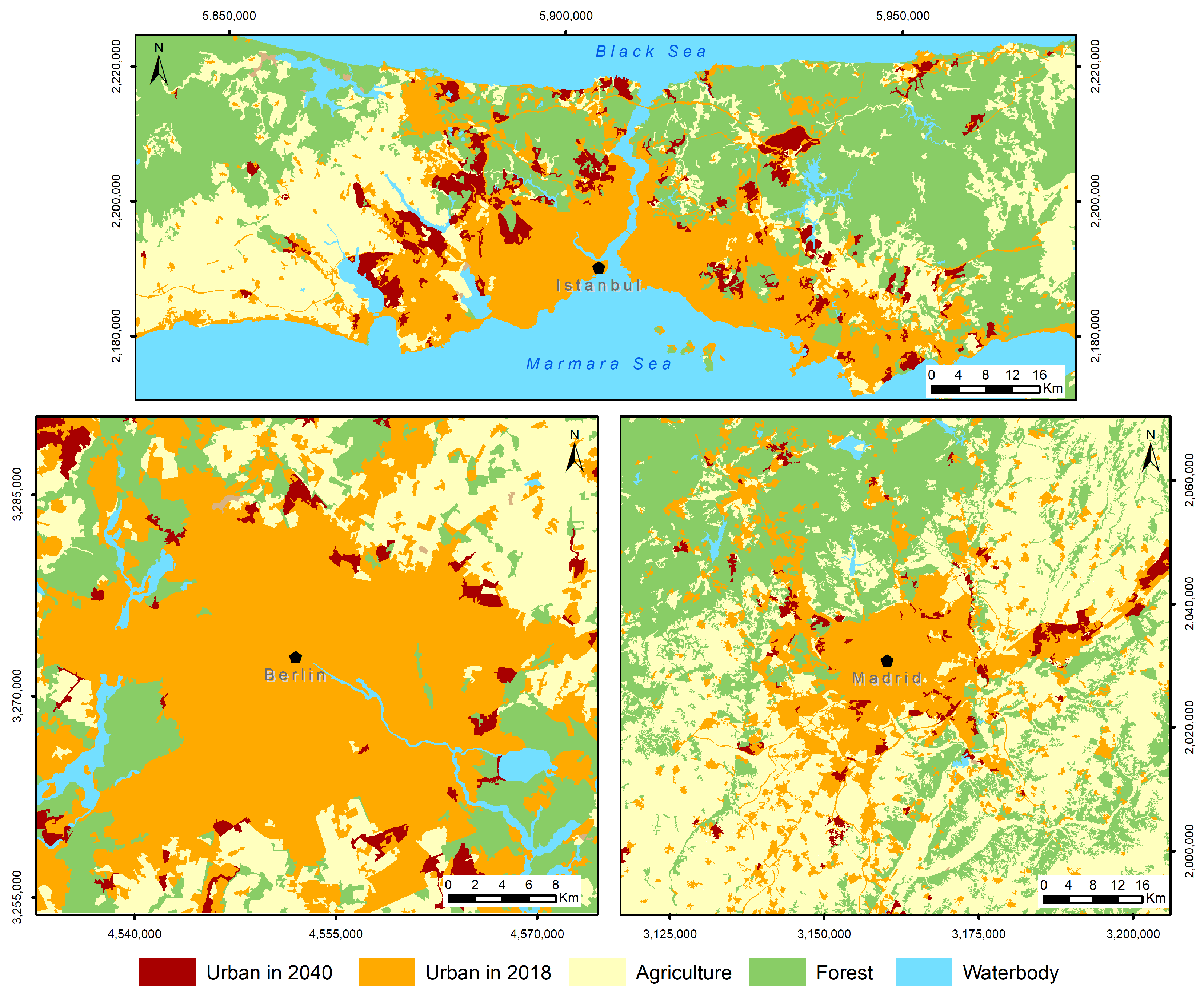
Nine different VCA-ML-based UGSMs were developed as part of this study. The joint urban growth areas identified in the VCA-RF, VCA-SVM, and VCA-MLP models for the year 2040 were analyzed to identify agricultural and forest lands with high potential for urbanization (Figure 7). This approach aimed to create more accurate simulation models. Therefore, the transformation rates of the wetlands located in the study areas are not included in

Table 4. LULC change detection results (2018–2040) derived from VCA-ML intersection UGSM.

LULC Class	Istanbul			Berlin			Madrid
	Area (ha)	(+)	(−)	Area (ha)	(+)	(−)	Area (ha)	(+)	(−)
Urban	11,469.1	8.2%		5614.8	4.2%		8784.1	6.3%
Agriculture	7755.3		4.8%	4174.7		10.0%	7230.5		1.5%
Forest	3713.8		1.4%	1440.1		4.5%	1553.6		0.4%

and Figure 7 due to their negligible importance.

The results from the change detection analysis conducted between 2018 and 2040 indicated an estimated urban growth probability of 8.2% in Istanbul, 4.2% in Berlin, and 6.3% in Madrid (Table 4). In Istanbul, considered a forest-intensive study area, agricultural land is at a risk of urbanization about twice that of forested areas. Similarly, significant growth is expected to be mainly in agricultural regions. In Madrid, the potential for agricultural areas to be converted into residential zones is approximately five times greater than for forested areas.

5. Discussion

This study presents a VCA-based UGSM to simulate changes in LULC driven by urban growth. The input data required for the model, which integrates three different ML algorithms, was sourced from open data repositories. For land cover data, we utilized the first level of the CORINE dataset. Accessibility data was obtained from the OSM and Google Earth services, while the 30-m resolution SRTM data provided the DEM necessary to create the slope map. Unlike previous VCA-based UGSM studies, which typically used high-resolution data, this research aims to model larger study areas using freely available, low-resolution open-source data with the VCA algorithm.

The paper introduces a new approach to the CA neighborhood and transformation rule components using the GV method. Unlike previous methods developed for VCA, our findings suggest that the proposed GV method serves as a feasible alternative that can be adapted to diverse study areas. The method offers a flexible structure that enables accurate modeling of real-world geographic features.

We also analyzed the distance of local influence between polygons through temporal geographic variance. The histogram of the base lengths of the GVs that generate temporal urbanization in all study areas closely follows a gamma probability distribution. In this framework, the optimal distance point is found in the right tail of the distribution, allowing us to identify a value that is both higher than the mean and distinctly separated from outliers. Thus, unlike previous studies, our model can establish the maximum distance value for urban growth based on local conditions rather than relying on an empirical approach.

In the proposed model, the generated GVs define the zone of influence for each polygon, with the neighborhoods represented as polygons within these zones. Between 1990 and 2018, during four distinct periods, a total of 17,872 temporal GVs were identified in Istanbul, 21,635 in Berlin, and 41,831 in Madrid. Among these, 5675 in Istanbul, 7841 in Berlin, and 9481 in Madrid were unclassified GVs that contributed to urbanization.

The number of GVs obtained is related to both the number of polygons and the number of neighborhoods within the study area. Although calculations in this study were performed on a single core using a powerful computer with high-performance capabilities and low-resolution data, the number of GVs is expected to increase when the model is applied to parcel-based high-resolution data. To address this, integrating methods such as multi-threading or multiprocessing architectures, utilizing CUDA-supported GPU computing or asynchronous programming, could significantly reduce processing time.

The developed model incorporates the modeling capabilities of VCA along with calibration and validation stages that highlight the differences between actual and simulated urban growth. Both phases allow for model training, validation, and selection using VCA and three ML algorithms over 28-year time intervals. The results indicate that the RF algorithm provides the best performance across all cities. Our findings demonstrate that the model, despite using low-resolution data, can achieve high accuracy when the RF algorithm is employed. The training stage achieved an average accuracy of 0.83 with the SVM algorithm and 0.85 with the MLP algorithm. Compared to similar studies in the literature, the accuracy value for SVM was found to improve slightly, while similar results were obtained for MLP [20,58].

We conducted an ROC curve analysis during the model validation phase and calculated AUC values to guide our model selection. It was found that the VCA-RF model exhibited the highest AUC value and demonstrated the most successful predictions across all three cities. While the performance differences between the VCA-SVM and VCA-MLP models varied from city to city, it was determined that all three models performed more effectively in Madrid compared to the other cities.

The proposed model presents several limitations that warrant further investigation. One key limitation is the representation of time in CA-based models; each VCA-ML loop in the model represents a single year, while LULC transformations may not occur within the same timeframe, as LULC changes are process-oriented. Future works should focus on modeling the time dimension more accurately. Additionally, the absence of a self-modification algorithm that stabilizes the growth rate indicates that the growth rate should be adjusted based on historical annual rates for greater stability. The model has been tested using low-resolution vector data and parcel-based studies conducted within planning units are planned in the future to produce a precise model.

This study also explores the effects of GV parameters applied in Istanbul, Berlin, and Madrid. The findings indicate that GV direction is the most effective parameter across all models, with directional information consistently proving significant in various study areas. While other parameters, such as cell area and edge effect, also contribute to the modeling, their impact varies depending on the study area and algorithm used. The consistent result of the GV direction parameter highlights the potential of the proposed model for application in diverse fields of study.

During the simulation phase, the VCA-RF, VCA-SVM, and VCA-MLP models were overlapped, and intersecting polygons were found to increase the prediction accuracy and identify regions with high LULC transformation potential. The change detection analysis indicates that urban growth potential in Istanbul is projected to reach 8.19% by 2040. Ayazlı et al. created a UGSM for 2040 based on a similar scenario. A comparison of the results from both models shows changes occurring in similar regions of Istanbul [59]. Notably, the northern forests of Istanbul are under pressure from urbanization in both models, particularly around the Yavuz Sultan Selim Bridge and Istanbul Airport, which show significant potential for urban development and related land cover changes.

In Berlin, the implementation of green growth policies aims to promote sustainability; however, these policies have led to losses in agricultural and forest areas due to LULC changes, primarily driven by population growth and housing shortages since 2016 [60,61]. Our findings align with these studies. According to our proposed model, we determined an urban growth probability of 4.18% in Berlin, assessed in terms of urban density.

In Madrid, simulations for 2040 indicate an urban growth potential of 6.34%. The model results suggest that these growth areas pose significant risks, particularly affecting 7231 hectares of agricultural land. The literature on LULC change indicates that urban areas may expand in response to increasing population growth and transport infrastructure development [62,63].

6. Conclusions

This study examines land cover changes driven by urban growth using a new VCA-based simulation model. The calibration results demonstrate the model’s effectiveness in capturing macro-scale LULC dynamics and generating significant insights. A key innovation of this approach lies in its ability to model dynamic neighborhood relationships through the concept of GVs defined over time, integrating these GVs with ML algorithms such as RF, SVM, and MLP. The results indicate that the proposed VCA-based model can detect LULC changes, even when using low-resolution data, across different study areas.

In conclusion, the proposed VCA-based UGSM model is a generalizable and reliable tool for simulating urban growth. It can adapt to various spatial resolutions and LULC dynamics while utilizing open-source data. The model’s effectiveness in cities with diverse structures, such as Istanbul, Berlin, and Madrid, demonstrates its international applicability. Future works will aim to enhance the model by integrating social, economic, and political variables into the GV parameterization and improving the calibration and time components to increase accuracy.