

A Network Approach for Discovering Spatially Associated Objects
 , , , and
Abstract
1. Introduction
- The maximum topological accessibility path was developed to quantify objects’ similarity attenuation along topological lines.
- The WSTA approach was proposed by integrating topological accessibility into the network model.
- This study demonstrates the effectiveness and suitability of WSTA by validating it using the Beijing POI dataset. The results show that WSTA leads to a significant improvement in accuracy when considering spatial topology.
2. Related Studies
2.1. Discovering Spatially Associated Object Methods
2.2. Involvement of Spatial Topology in Discovering Associated Objects
3. Study Area and Data
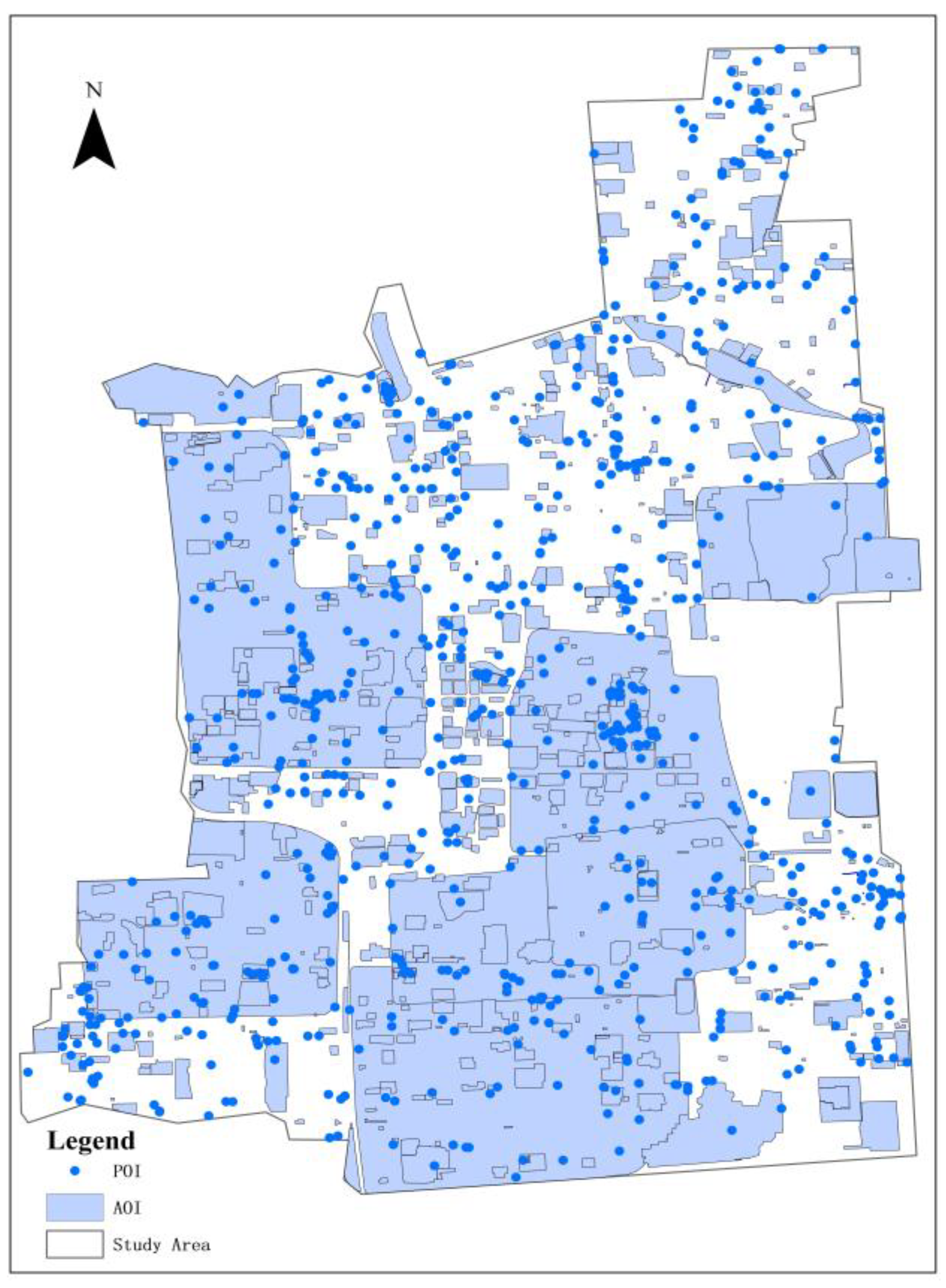
3.1. Study Area and Data Preprocessing
3.2. Benchmark Dataset
4. Methodology
4.1. Design Principles and Considerations
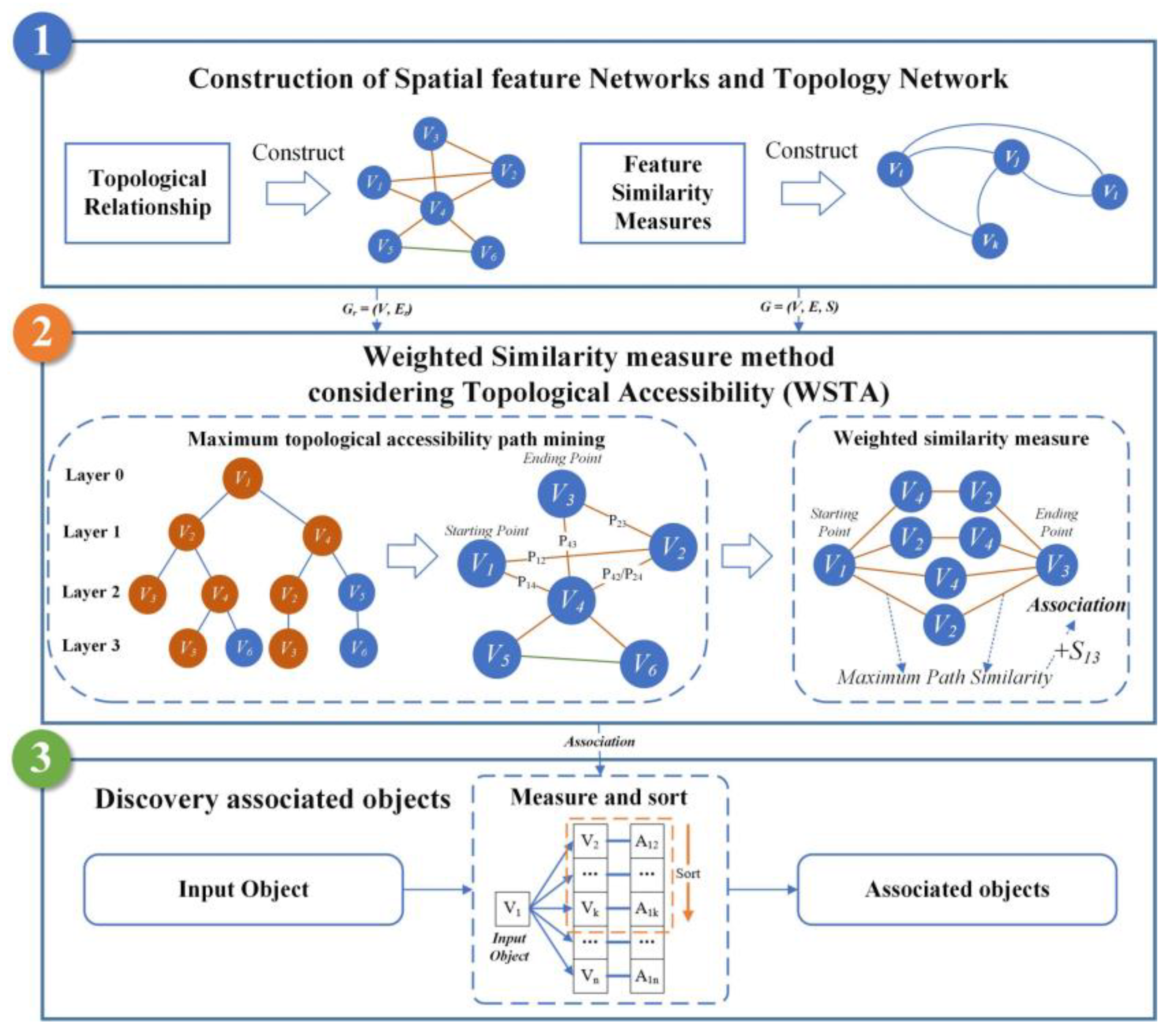
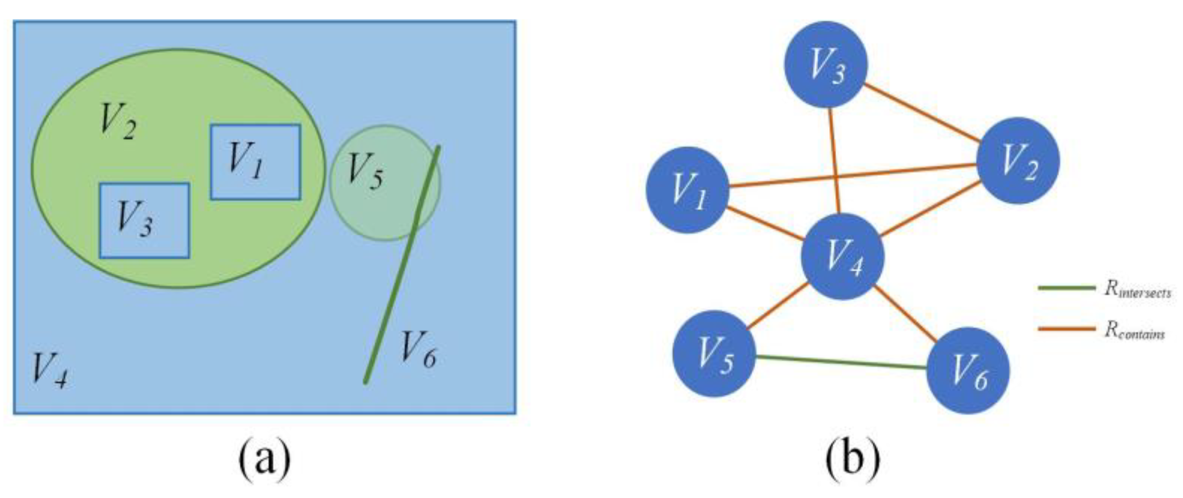
4.2. Construction of Network Model
4.2.1. Constructing a Spatial Feature Similarity Network
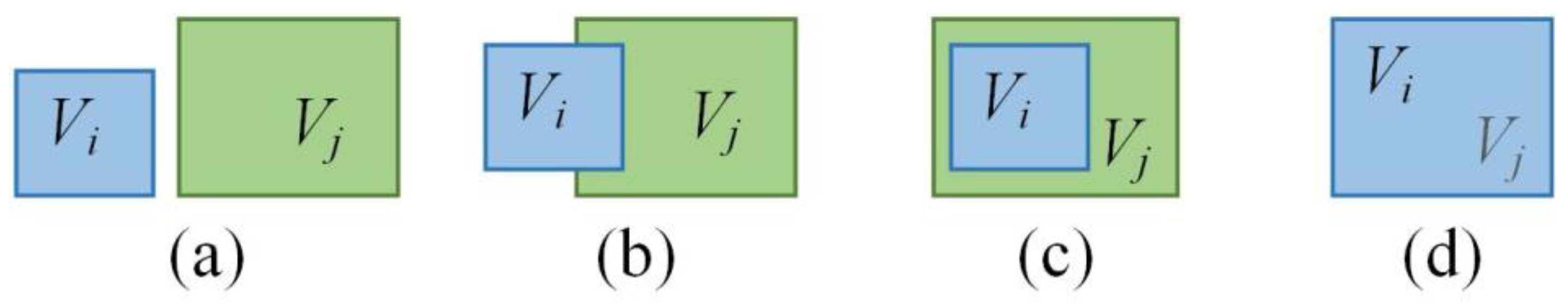
4.2.2. Construction of a Topology Network
4.3. Weighted Similarity Measure Method Considering Topological Accessibility
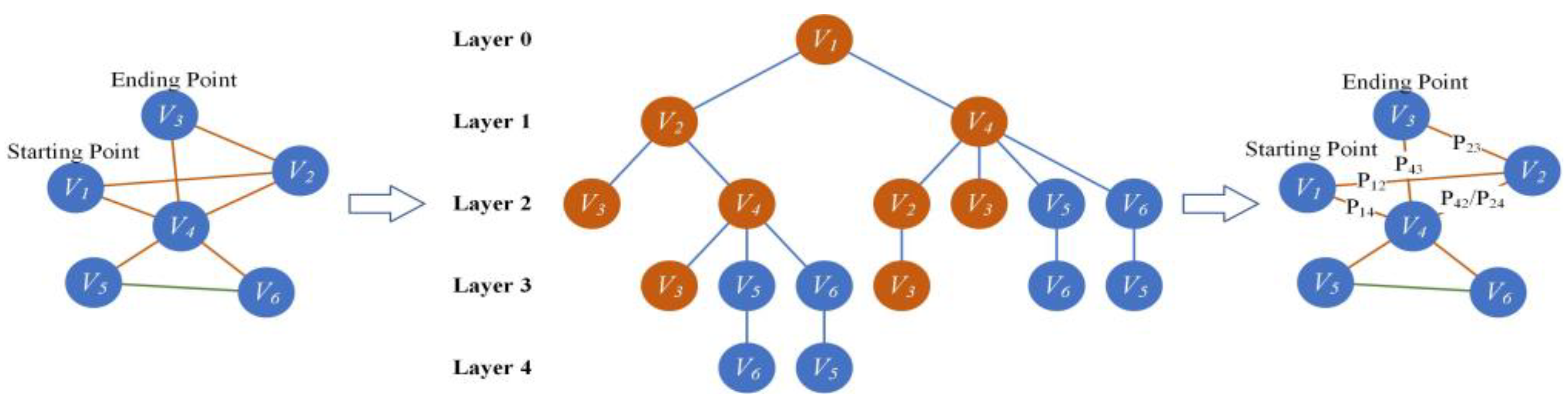
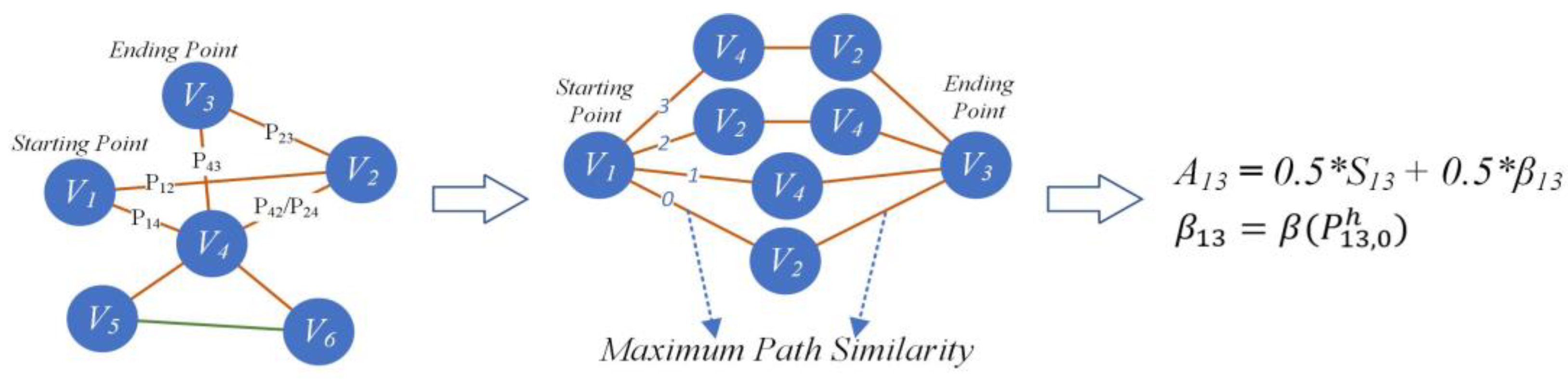
4.3.1. Maximum Topological Accessibility Path
4.3.2. Weighted Association Calculation
5. Experiments and Results
5.1. Experimental Parameter Configuration
5.1.1. Network Construction Parameters
5.1.2. Baseline Methods
- Baseline 1 [18]. This method is based on spatial topological relationship, and we fully considered its influence on the object spatial association measure. In our study, the association factor parameter in this method is set to one.
- Baseline 2 [14]. The normalized topological relationships and metrics were employed to express the degree of object spatial association. Its advantage is its multiple-scale capability.
- Baseline 3 [13]. Adaptive topological relationships and metric thresholds according to object types are directly used to measure object spatial association. Considering the spatial scale in our study, 500 m was selected as the spatial filter unit parameter.
- Baseline 4 [19]. The principle of this method is spatial clustering. The associated objects were retrieved from clusters with specific conditions. The advantages of this method are its efficiency and accuracy. Based on the literature results, the DBSCAN spatial clustering algorithm was used in our study.
5.1.3. Evaluation Methods and Indicators
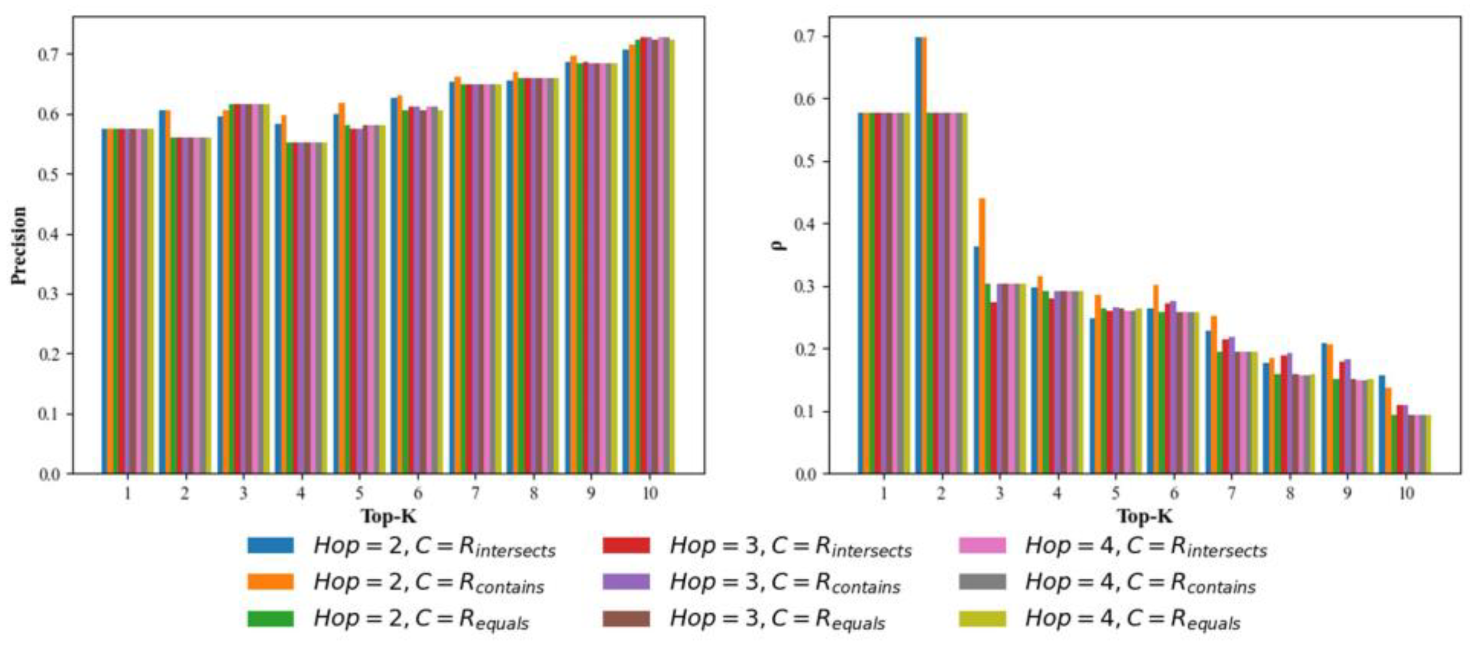
5.2. The Top-K Results
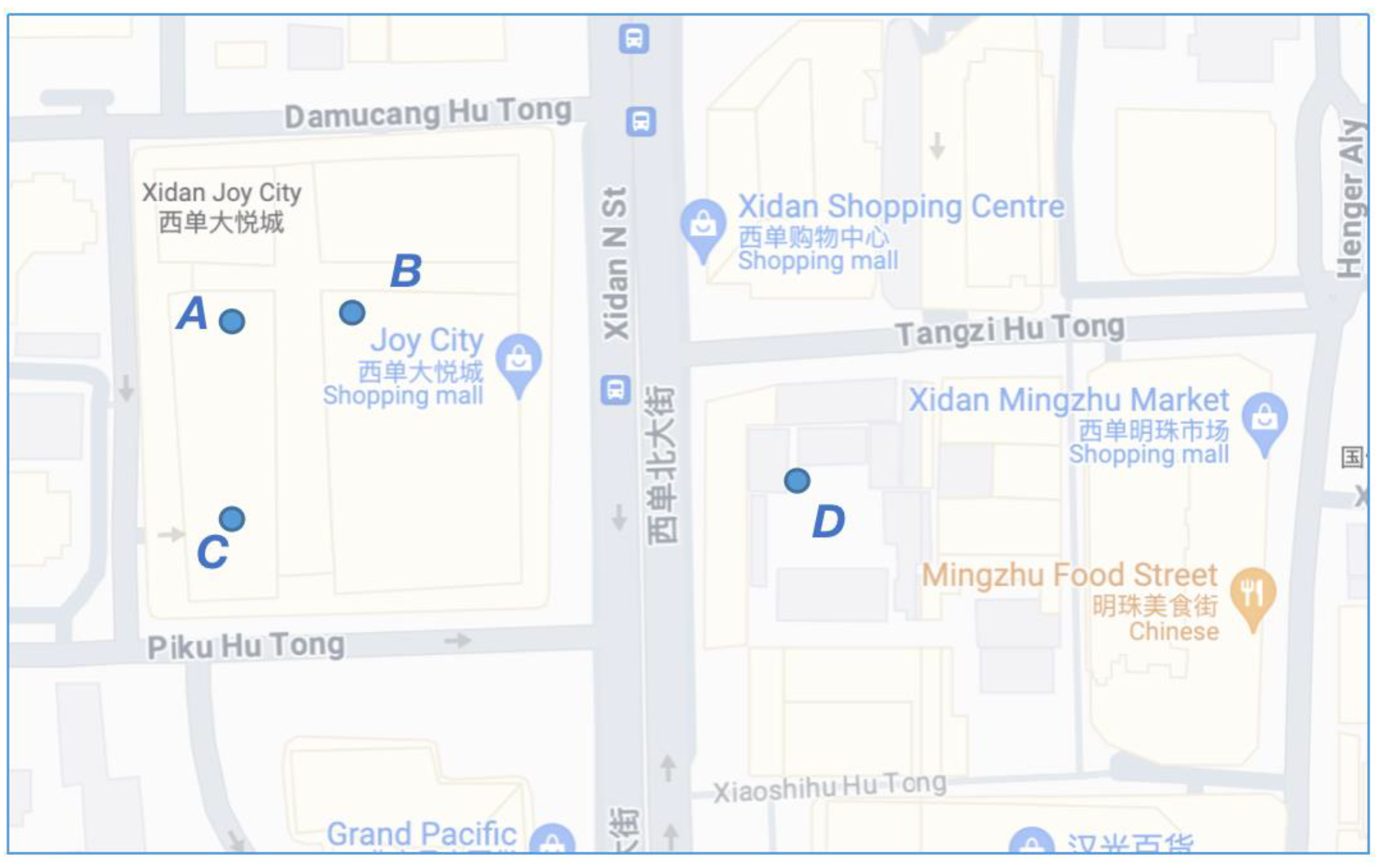
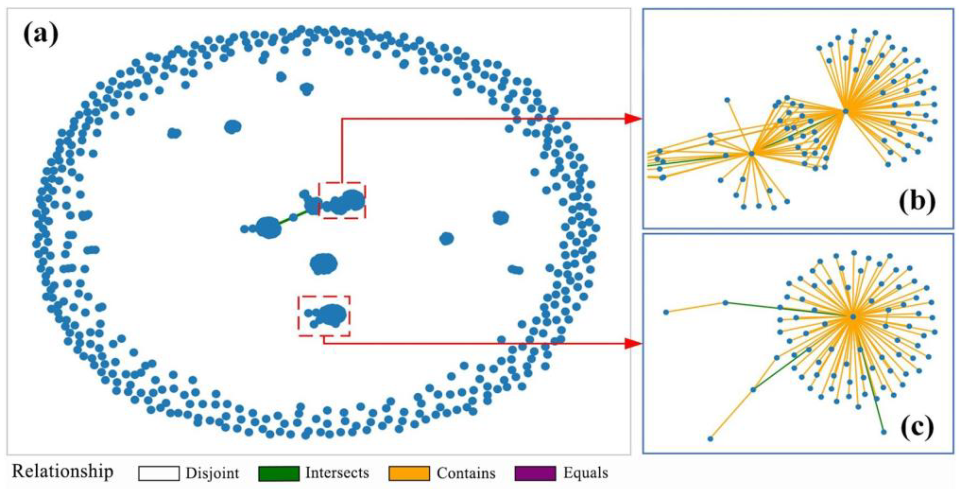
5.2.1. Case Study for Associated Object Discovery
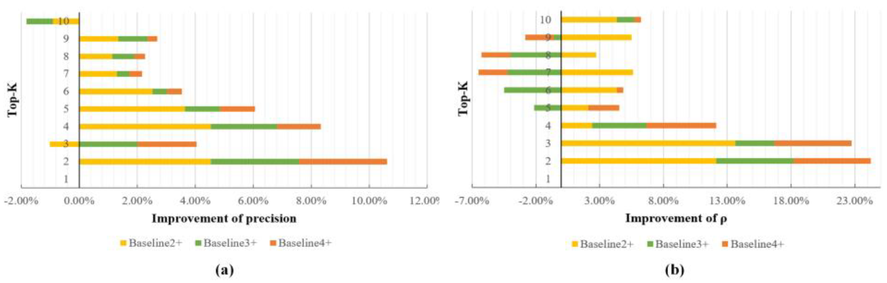
5.2.2. Accuracy Comparison Results of Methods
6. Discussion
6.1. Suitability Analysis
6.2. Performance Analysis Integrating WSTA
7. Conclusions
Author Contributions
Funding
Data Availability Statement
Acknowledgments
Conflicts of Interest
References
- Wiemann, S.; Bernard, L. Spatial Data Fusion in Spatial Data Infrastructures Using Linked Data. Int. J. Geogr. Inf. Sci. 2016, 30, 613–636. [Google Scholar] [CrossRef]
- Song, Y. The Second Dimension of Spatial Association. Int. J. Appl. Earth Obs. Geoinf. 2022, 111, 102834. [Google Scholar] [CrossRef]
- Chen, N.; Yang, A.; Chen, L.; Xiong, W.; Jing, N. STO2Vec: A Multiscale Spatio-Temporal Object Representation Method for Association Analysis. ISPRS Int. J. Geo-Inf. 2023, 12, 207. [Google Scholar] [CrossRef]
- Yan, T.; Mistry, M.; Krzyś, K.; Castelhano, M. Searching for the Cat: Effects of Variable Spatial Association between Objects and Scenes. J. Vision 2020, 20, 1614. [Google Scholar] [CrossRef]
- Tobler, W.R. A Computer Movie Simulating Urban Growth in the Detroit Region. Econ. Geogr. 1970, 46, 234–240. [Google Scholar] [CrossRef]
- Berners-Lee, T.; Hendler, J.; Lassila, O. The Semantic Web: A New Form of Web Content That Is Meaningful to Computers Will Unleash a Revolution of New Possibilities. In Linking the World’s Information: Essays on Tim Berners-Lee’s Invention of the World Wide Web; ACM: New York, NY, USA, 2023; pp. 91–103. [Google Scholar]
- Cox, S.J. An Explicit OWL Representation of ISO/OGC Observations and Measurements. In Proceedings of the 6th International Conference on Semantic Sensor Networks, Sydney, Australia, 22 October 2013; pp. 1–18. [Google Scholar]
- Hamdi, A.; Shaban, K.; Erradi, A.; Mohamed, A.; Rumi, S.K.; Salim, F.D. Spatiotemporal Data Mining: A Survey on Challenges and Open Problems. Artif. Intell. Rev. 2022, 55, 1441–1488. [Google Scholar] [CrossRef] [PubMed]
- Appice, A.; Ceci, M.; Lanza, A.; Lisi, F.A.; Malerba, D. Discovery of Spatial Association Rules in Geo-Referenced Census Data: A Relational Mining Approach. Intell. Data Anal. 2003, 7, 541–566. [Google Scholar] [CrossRef]
- He, Z.; Deng, M.; Cai, J.; Xie, Z.; Guan, Q.; Yang, C. Mining Spatiotemporal Association Patterns from Complex Geographic Phenomena. Int. J. Geogr. Inf. Sci. 2020, 34, 1162–1187. [Google Scholar] [CrossRef]
- Zhou, L.; Wang, C.; Zhen, F. Exploring and Evaluating the Spatial Association between Commercial and Residential Spaces Using Baidu Trajectory Data. Cities 2023, 141, 104514. [Google Scholar] [CrossRef]
- Wang, D.; Tong, X.; Dai, C.; Guo, C.; Lei, Y.; Qiu, C.; Li, H.; Sun, Y. Voxel Modeling and Association of Ubiquitous Spatiotemporal Information in Natural Language Texts. Int. J. Digit. Earth 2023, 16, 868–890. [Google Scholar] [CrossRef]
- Guo, L.; Jiang, J.; Li, H.; Wang, Y. Analysis of multi-source geospatial vector data association. Bull. Surv. Mapp. 2020, 6, 71–76+86. [Google Scholar] [CrossRef]
- Zhao, H.; Zhu, Y.; Hou, Z.; Yang, H. Construction of Geospatial Metadata Association Network. Sci. Geogr. Sin. 2016, 36, 1180–1189. [Google Scholar]
- Jiang, J.; Xu, J.; Lou, Y. Spatial Line Entity Matching Technology for Spatial Association of Multi-Source Vector Data. In Proceedings of the 2022 3rd International Conference on Big Data, Artificial Intelligence and Internet of Things Engineering (ICBAIE), Xi’an, China, 15–17 July 2022; IEEE: Piscataway, NJ, USA, 2022; pp. 523–527. [Google Scholar]
- De Sabbata, S.; Reichenbacher, T. Criteria of Geographic Relevance: An Experimental Study. Int. J. Geogr. Inf. Sci. 2012, 26, 1495–1520. [Google Scholar] [CrossRef]
- Wu, Y.; Chen, L.; Xiong, W.; Zhong, Z.; Jing, N. Multi-Source Geospatial Data Correlation Model for Efficient Retrieval. Chin. J. Comput. 2014, 9, 1999–2010. [Google Scholar]
- Han, B. Research on Multi-Source Remote Sensing Image Correlation for Retrieval. Master’s Thesis, Graduate School of National University of Defense Technology, Changsha, China, 2012. [Google Scholar]
- Wang, D.; Cui, W.; Qin, B. Graph Compression Storage Based on Spatial Cluster Entity Optimization. IEEE Access 2020, 8, 29075–29088. [Google Scholar] [CrossRef]
- Xu, Y.; Xie, Z.; Chen, Z.; Wu, L. Shape Similarity Measurement Model for Holed Polygons Based on Position Graphs and Fourier Descriptors. Int. J. Geogr. Inf. Sci. 2017, 31, 253–279. [Google Scholar] [CrossRef]
- Xu, Y.; Xie, Z.; Chen, Z.; Xie, M. Measuring the Similarity between Multipolygons Using Convex Hulls and Position Graphs. Int. J. Geogr. Inf. Sci. 2021, 35, 847–868. [Google Scholar] [CrossRef]
- Zhu, Y.; Zhu, A.-X.; Feng, M.; Song, J.; Zhao, H.; Yang, J.; Zhang, Q.; Sun, K.; Zhang, J.; Yao, L. A Similarity-Based Automatic Data Recommendation Approach for Geographic Models. Int. J. Geogr. Inf. Sci. 2017, 31, 1403–1424. [Google Scholar] [CrossRef]
- Liao, W.; Hou, D.; Jiang, W. An Approach for a Spatial Data Attribute Similarity Measure Based on Granular Computing Closeness. Appl. Sci. 2019, 9, 2628. [Google Scholar] [CrossRef]
- Purves, R.S.; Clough, P.; Jones, C.B.; Arampatzis, A.; Bucher, B.; Finch, D.; Fu, G.; Joho, H.; Syed, A.K.; Vaid, S.; et al. The Design and Implementation of SPIRIT: A Spatially Aware Search Engine for Information Retrieval on the Internet. Int. J. Geogr. Inf. Sci. 2007, 21, 717–745. [Google Scholar] [CrossRef]
- Janowicz, K.; Raubal, M.; Kuhn, W. The Semantics of Similarity in Geographic Information Retrieval. J. Spat. Inf. Sci. 2011, 2, 29–57. [Google Scholar] [CrossRef]
- Hu, S.; Xing, H.; Luo, W.; Wu, L.; Xu, Y.; Huang, W.; Liu, W.; Li, T. Uncovering the Association between Traffic Crashes and Street-Level Built-Environment Features Using Street View Images. Int. J. Geogr. Inf. Sci. 2023, 37, 2367–2391. [Google Scholar] [CrossRef]
- Liu, Y.; Wang, F.; Kang, C.; Gao, Y.; Lu, Y. Analyzing Relatedness by Toponym Co-O Ccurrences on Web Pages. Trans. GIS 2014, 18, 89–107. [Google Scholar] [CrossRef]
- Yuan, Z. A Nonparametric Approach to Measure the Heterogeneous Spatial Association: Under Spatial Temporal Data. arXiv 2018, arXiv:1803.02334. [Google Scholar]
- Kim, J.O.; Yu, K.; Heo, J.; Lee, W.H. A New Method for Matching Objects in Two Different Geospatial Datasets Based on the Geographic Context. Comput. Geosci. 2010, 36, 1115–1122. [Google Scholar] [CrossRef]
- Sierra, R.; Stephens, C.R. Exploratory Analysis of the Interrelations between Co-Located Boolean Spatial Features Using Network Graphs. Int. J. Geogr. Inf. Sci. 2012, 26, 441–468. [Google Scholar] [CrossRef]
- Chen, Y.; Xu, J.; Xu, M. Finding Community Structure in Spatially Constrained Complex Networks. Int. J. Geogr. Inf. Sci. 2015, 29, 889–911. [Google Scholar] [CrossRef]
- Jiang, B.; Ren, Z. Geographic Space as a Living Structure for Predicting Human Activities Using Big Data. Int. J. Geogr. Inf. Sci. 2019, 33, 764–779. [Google Scholar] [CrossRef]
- Lu, X.; Li, H.; Xu, Y.; Liu, J.; Chen, Z. Measuring the Similarity between Shapes of Buildings Using Graph Edit Distance. Int. J. Digit. Earth 2024, 17, 2310749. [Google Scholar] [CrossRef]
- Yan, M.; Zhong, Z.; Jing, N.; Wu, Y. Method for Calculating Geographic Entity Relevance Based on Spatial and Semantic Association. In Proceedings of the 2019 International Conference on Data Mining Workshops (ICDMW), Beijing, China, 8–11 November 2019; IEEE: Piscataway, NJ, USA, 2019; pp. 490–496. [Google Scholar]
- Rottoli, G.D.; Merlino, H. Spatial Association Discovery Process Using Frequent Subgraph Mining. Telkomnika 2020, 18, 1884. [Google Scholar] [CrossRef]
- Xu, H.; Jiang, C.; Liang, X.; Li, Z. Spatial-Aware Graph Relation Network for Large-Scale Object Detection. In Proceedings of the IEEE/CVF Conference on Computer Vision and Pattern Recognition, Long Beach, CA, USA, 15–20 June 2019; pp. 9298–9307. [Google Scholar]
- Zhang, W.-B.; Ge, Y.; Leung, Y.; Zhou, Y. A Georeferenced Graph Model for Geospatial Data Matching by Optimising Measures of Similarity across Multiple Scales. Int. J. Geogr. Inf. Sci. 2021, 35, 2339–2355. [Google Scholar] [CrossRef]
- Sun, Y.; Han, J.; Yan, X.; Yu, P.S.; Wu, T. Pathsim: Meta Path-Based Top-k Similarity Search in Heterogeneous Information Networks. Proc. VLDB Endow. 2011, 4, 992–1003. [Google Scholar] [CrossRef]
- Schneider, M.; Behr, T. Topological Relationships between Complex Spatial Objects. ACM Trans. Database Syst. (TODS) 2006, 31, 39–81. [Google Scholar] [CrossRef]
- Borrmann, A.; Rank, E. Topological Analysis of 3D Building Models Using a Spatial Query Language. Adv. Eng. Inform. 2009, 23, 370–385. [Google Scholar] [CrossRef]
- Majumdar, S.; Laha, A.K. Clustering and Classification of Time Series Using Topological Data Analysis with Applications to Finance. Expert Syst. Appl. 2020, 162, 113868. [Google Scholar] [CrossRef]
- Corcoran, P.; Jones, C.B. Topological Data Analysis for Geographical Information Science Using Persistent Homology. Int. J. Geogr. Inf. Sci. 2023, 37, 712–745. [Google Scholar] [CrossRef]
- Alomari, H.W.; Al-Badarneh, A.F.; Al-Alaj, A.; Khamaiseh, S.Y. Enhanced Approach for Agglomerative Clustering Using Topological Relations. IEEE Access 2023, 11, 21945–21967. [Google Scholar] [CrossRef]
- Nguyen, T.T.; Nguyen, L.T.; Bui, Q.-T.; Yun, U.; Vo, B. An Efficient Topological-Based Clustering Method on Spatial Data in Network Space. Expert Syst. Appl. 2023, 215, 119395. [Google Scholar] [CrossRef]
- Clementini, E.; Sharma, J.; Egenhofer, M.J. Modelling Topological Spatial Relations: Strategies for Query Processing. Comput. Graph. 1994, 18, 815–822. [Google Scholar] [CrossRef]
- Wu, Y.; Shang, J.; Hu, X.; Zhou, Z. Extended Maptree: A Representation of Fine-Grained Topology and Spatial Hierarchy of Bim. Int. Arch. Photogramm. Remote Sens. Spat. Inf. Sci. 2017, 42, 409–415. [Google Scholar] [CrossRef]
- Jing, C.; Zhu, Y.; Du, M.; Liu, X. Visualizing Spatiotemporal Patterns of City Service Demand through a Space-Time Exploratory Approach. Trans. GIS 2021, 25, 1766–1783. [Google Scholar] [CrossRef]
- Bizer, C.; Heath, T.; Berners-Lee, T. Linked Data-The Story So Far. Int. J. Semant. Web Inf. Syst. (IJSWIS) 2009, 5, 1–22. [Google Scholar] [CrossRef]
- Zhang, W. How to Construct the Statistic Network? An Association Network of Herbaceous Plants Constructed from Field Sampling. Netw. Biol. 2012, 2, 57. [Google Scholar]
- Leiserson, C.E.; Schardl, T.B. A Work-Efficient Parallel Breadth-First Search Algorithm (or How to Cope with the Nondeterminism of Reducers). In Proceedings of the Twenty-Second Annual ACM Symposium on Parallelism in Algorithms and Architectures, Thira Santorini, Greece, 13–15 June 2010; Association for Computing Machinery: New York, NY, USA, 2010; pp. 303–314. [Google Scholar]
- Saxena, A.; Gera, R.; Iyengar, S. A Heuristic Approach to Estimate Nodes’ Closeness Rank Using the Properties of Real World Networks. Soc. Netw. Anal. Min. 2019, 9, 3. [Google Scholar] [CrossRef]
- Fournier-Viger, P.; Wu, C.-W.; Tseng, V.S. Mining Top-K Association Rules. In Advances in Artificial Intelligence; Kosseim, L., Inkpen, D., Eds.; Lecture Notes in Computer Science; Springer: Berlin/Heidelberg, Germany, 2012; Volume 7310, pp. 61–73. ISBN 978-3-642-30352-4. [Google Scholar]
- Poonkuzhali, G.; Kumar, R.K.; Sudhakar, P.; Uma, G.V.; Sarukesi, K. Relevance Ranking and Evaluation of Search Results through Web Content Mining. Lect. Notes Eng. Comput. Sci. 2012, 2195, 456–460. [Google Scholar]
- Riyanto, S.; Sitanggang, I.S.; Djatna, T.; Atikah, T.D. Comparative Analysis Using Various Performance Metrics in Imbalanced Data for Multi-Class Text Classification. IJACSA 2023, 14, 1082–1090. [Google Scholar] [CrossRef]
- Sedgwick, P. Spearman’s Rank Correlation Coefficient. BMJ 2014, 349, g7327. [Google Scholar] [CrossRef]
- Reichenbacher, T.; De Sabbata, S.; Purves, R.S.; Fabrikant, S.I. Assessing Geographic Relevance for Mobile Search: A Computational Model and Its Validation via Crowdsourcing. J. Assoc. Inf. Sci. Technol. 2016, 67, 2620–2634. [Google Scholar] [CrossRef]
- Liu, S.; Zou, Y.; Terasvirta, A.M. Fast Query Algorithm for Social Network Data Based on Association Features. IFS 2018, 35, 4153–4162. [Google Scholar] [CrossRef]
- Shi, C.; Kong, X.; Huang, Y.; Yu, P.S.; Wu, B. HeteSim: A General Framework for Relevance Measure in Heterogeneous Networks. IEEE Trans. Knowl. Data Eng. 2014, 26, 2479–2492. [Google Scholar] [CrossRef]
- Scholer, F.; Williams, H.E. Query Association for Effective Retrieval. In Proceedings of the Eleventh International Conference on Information and Knowledge Management, McLean, VA, USA, 4–9 November 2002; ACM: New, York, USA, 2002; pp. 324–331. [Google Scholar]

| Method | No. 1 | No. 2 | No. 3 | No. 4 | No. 5 | No. 6 | No. 7 | No. 8 | No. 9 | No. 10 |
|---|---|---|---|---|---|---|---|---|---|---|
| Benchmark Results | A | B | C | D | E | F | G | H | I | J |
| Baseline 1 | A | E | C | D | G | B | H | F | I | L |
| Baseline 2 | A | C | D | G | B | H | F | I | E | J |
| Baseline 3 | A | C | D | G | B | H | F | E | I | J |
| Baseline 4 | A | C | D | G | B | H | F | I | J | K |
| Baseline 1+ | A | E | C | D | G | H | F | L | I | J |
| Baseline 2+ | A | D | C | B | E | G | I | F | H | J |
| Baseline 3+ | A | D | C | B | E | G | F | I | H | J |
| Baseline 4+ | A | D | C | B | G | F | I | H | J | K |
| Object ID | Name of Associated Objects | Walking Route in Gaode APP | Distance (Meters) |
|---|---|---|---|
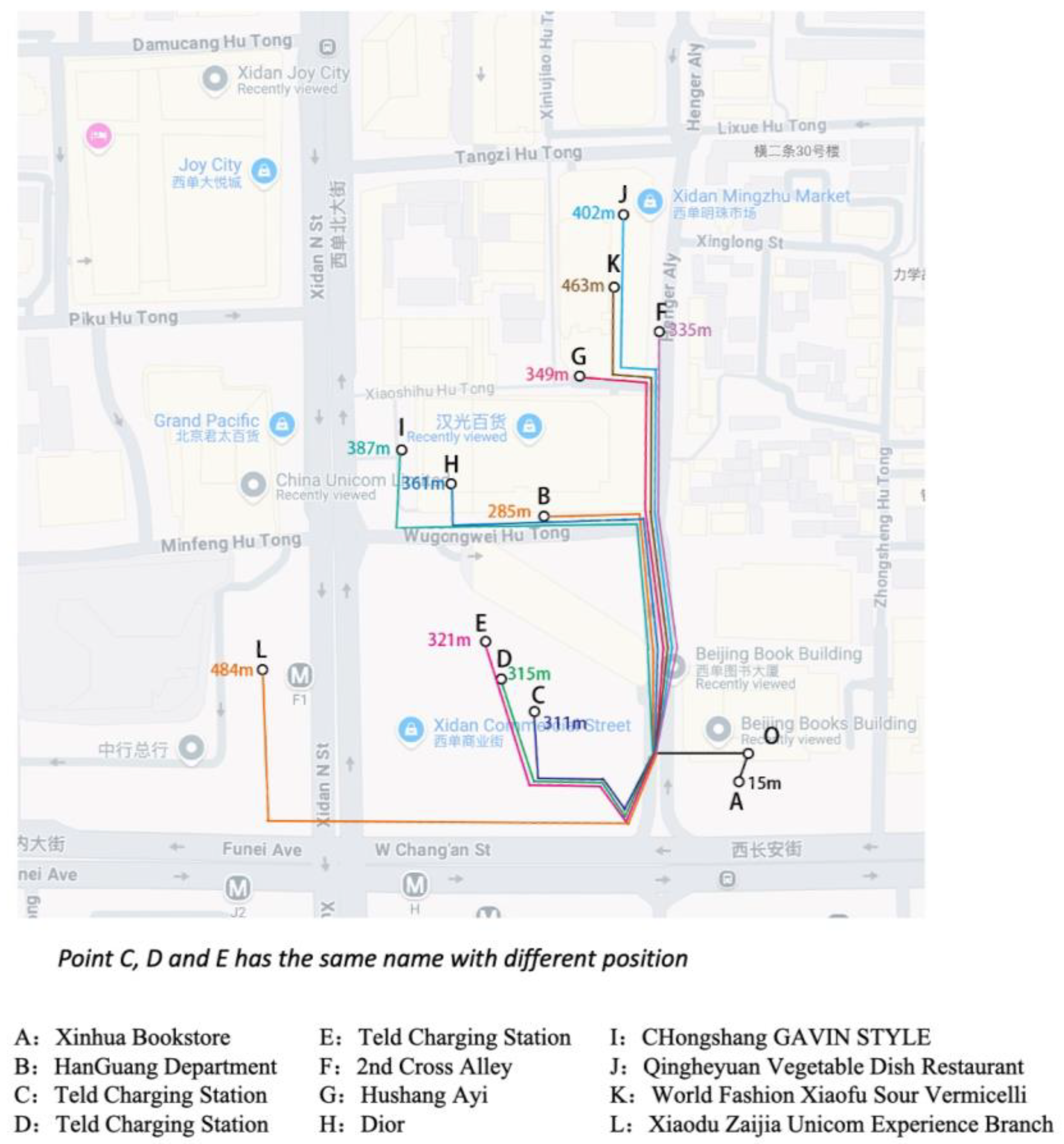
| A | Xinhua Bookstore (Beijing Books Building) | Head southwest 15 m to reach the destination. | 15 |
| B | HanGuang Department Store | Head 57 m and turn right, walk 72 m and turn right, walk 64 m north along the 2nd cross alley and turn left, walk 10 m and turn left, walk 82 m to reach the destination | 285 |
| C | Teld Charging Station (THE New Xidan Geng Xinchang) | Head 57 m and turn left, walk 42 m and turn right, walk 21 m north and turn left, walk 63 m west and turn right, walk 128 m to reach the destination | 311 |
| D | Teld Charging Station (Teld THE New Xidan Geng Xinchang) | Head 57 m and turnm left, walk 42 m and turn right, walk 21 m north and turn left, walk 63 m west and turn right, walk 132 m to reach the destination | 315 |
| E | Teld Charging Station (Teld THE New XidanGeng Xinchang) | Head 57 m and turn left, walk 42 m and turn right, walk 21 m north and turn left, walk 63 m west and turn right, walk 138 m to reach the destination | 321 |
| F | 2nd Cross Alley | Head 57 m and turn right, walk 72 m and turn right, walk 206 m north along the 2nd cross alley to reach the destination | 335 |
| G | Hushang Ayi (HanGuang Department Store) | Head 57 m and turn right, walk 72 m and turn right, walk 156 m north along the 2nd cross alley, turn left, walk 64 m west along Xiaoshihu Hutong to reach the destination | 349 |
| H | Dior (HanGuang Department Store) | Head 57 m and turn right, walk 72 m and turn right, walk 64 m north along the 2nd cross alley, turn left, walk 10 m and turn left, walk 123 m and turn right, walk 35 m to reach the destination | 361 |
| I | CHongshang GAVIN STYLE (HanGuang) | Head 57 m and turn right, walk 72 m and turn right, walk 64 m north along the 2nd cross alley, turn left, walk 10 m and turn left, walk 123 m and turn right, walk 61 m to reach the destination | 387 |
| J | Qingheyuan Vegetable Dish Restaurant (Gaodeng Mansion Shop) | Head 57 m and turn right, walk 72 m and turn right, walk 164 m north along the 2nd cross alley, walk to the left, walk 109 m to reach the destination | 402 |
| K | World Fashion Xiaofu Sour Vermicelli (Xidan Mingzhu Shopping Center Shop) | Head 57 m and turn right, walk 72 m and turn right, walk 278 m north along the 2nd cross alley, turn left, walk 56 m to reach the destination | 463 |
| L | Xiaodu Zaijia Unicom Experience Branch | Head 57 m and turn left, walk 42 m and walk to the right, walk 30 m southwest along the 2nd cross alley, walk to the right, walk 143 m west along West Chang’an Avenue, walk straight, walk 13 m west along Fuxingmen inner Street Building, walk to the right, walk 34 m, walk 165 m to reach the destination | 484 |
| Top-K | Top-1 | Top-2 | Top-3 | Top-4 | Top-5 | Top-6 | Top-7 | Top-8 | Top-9 | Top-10 |
|---|---|---|---|---|---|---|---|---|---|---|
| Method | Precision | Precision | Precision | Precision | Precision | Precision | Precision | Precision | Precision | Precision |
| ρ | ρ | ρ | ρ | ρ | ρ | ρ | ρ | ρ | ρ | |
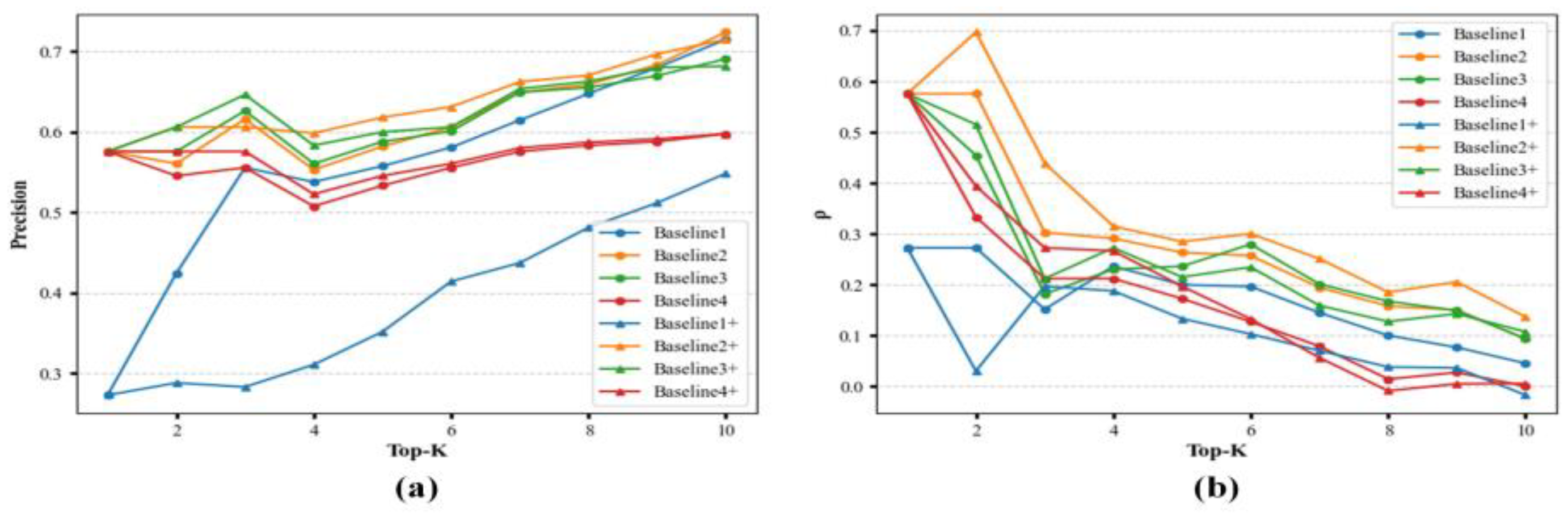
| Baseline 1 | 0.2727 | 0.4242 | 0.5556 | 0.5379 | 0.5576 | 0.5808 | 0.6147 | 0.6477 | 0.6801 | 0.7152 |
| 0.2727 | 0.2727 | 0.1515 | 0.2364 | 0.2 | 0.1965 | 0.145 | 0.1003 | 0.0768 | 0.0454 | |
| Baseline 2 | 0.5758 | 0.5606 | 0.6162 | 0.553 | 0.5818 | 0.6061 | 0.6494 | 0.6591 | 0.6835 | 0.7242 |
| 0.5758 | 0.5758 | 0.303 | 0.2909 | 0.2636 | 0.2571 | 0.1948 | 0.158 | 0.1505 | 0.0935 | |
| Baseline 3 | 0.5758 | 0.5758 | 0.6263 | 0.5606 | 0.5879 | 0.601 | 0.6494 | 0.6553 | 0.67 | 0.6909 |
| 0.5758 | 0.4545 | 0.1818 | 0.2303 | 0.2364 | 0.2797 | 0.2013 | 0.1674 | 0.149 | 0.0938 | |
| Baseline 4 | 0.5758 | 0.5455 | 0.5556 | 0.5076 | 0.5333 | 0.5556 | 0.5758 | 0.5833 | 0.588 | 0.5977 |
| 0.5758 | 0.3333 | 0.2121 | 0.2121 | 0.1727 | 0.1273 | 0.079 | 0.0144 | 0.0274 | 0.0003 | |
| Baseline 1+ | 0.2727 | 0.2879 | 0.2828 | 0.3106 | 0.3515 | 0.4141 | 0.4372 | 0.4811 | 0.5118 | 0.5485 |
| 0.2727 | 0.0303 | 0.197 | 0.1879 | 0.1333 | 0.103 | 0.0703 | 0.0382 | 0.0364 | −0.0171 | |
| Baseline 2+ | 0.5758 | 0.6061 | 0.6061 | 0.5985 | 0.6182 | 0.6313 | 0.6623 | 0.6705 | 0.697 | 0.7152 |
| 0.5758 | 0.697 | 0.4394 | 0.3152 | 0.2848 | 0.3004 | 0.2511 | 0.1854 | 0.2056 | 0.1368 | |
| Baseline 3+ | 0.5758 | 0.6061 | 0.6465 | 0.5833 | 0.6 | 0.6061 | 0.6537 | 0.6629 | 0.6801 | 0.6818 |
| 0.5758 | 0.5152 | 0.2121 | 0.2727 | 0.2152 | 0.2346 | 0.1591 | 0.1277 | 0.1429 | 0.1074 | |
| Baseline 4+ | 0.5758 | 0.5758 | 0.5758 | 0.5227 | 0.5455 | 0.5606 | 0.5801 | 0.5871 | 0.5913 | 0.5977 |
| 0.5758 | 0.3939 | 0.2727 | 0.2667 | 0.197 | 0.1325 | 0.0563 | −0.0087 | 0.0052 | 0.0058 |
Disclaimer/Publisher’s Note: The statements, opinions and data contained in all publications are solely those of the individual author(s) and contributor(s) and not of MDPI and/or the editor(s). MDPI and/or the editor(s) disclaim responsibility for any injury to people or property resulting from any ideas, methods, instructions or products referred to in the content. |
© 2025 by the authors. Published by MDPI on behalf of the International Society for Photogrammetry and Remote Sensing. Licensee MDPI, Basel, Switzerland. This article is an open access article distributed under the terms and conditions of the Creative Commons Attribution (CC BY) license (https://creativecommons.org/licenses/by/4.0/).
Share and Cite
Jing, C.; Liang, T.; Feng, Y.; Li, J.; Wu, S.; Ding, J.; Xu, G.; Hu, Y. A Network Approach for Discovering Spatially Associated Objects. ISPRS Int. J. Geo-Inf. 2025, 14, 226. https://doi.org/10.3390/ijgi14060226
Jing C, Liang T, Feng Y, Li J, Wu S, Ding J, Xu G, Hu Y. A Network Approach for Discovering Spatially Associated Objects. ISPRS International Journal of Geo-Information. 2025; 14(6):226. https://doi.org/10.3390/ijgi14060226
Chicago/Turabian StyleJing, Changfeng, Tao Liang, Yunlong Feng, Jianing Li, Sensen Wu, Jiale Ding, Gaoran Xu, and Yang Hu. 2025. "A Network Approach for Discovering Spatially Associated Objects" ISPRS International Journal of Geo-Information 14, no. 6: 226. https://doi.org/10.3390/ijgi14060226
APA StyleJing, C., Liang, T., Feng, Y., Li, J., Wu, S., Ding, J., Xu, G., & Hu, Y. (2025). A Network Approach for Discovering Spatially Associated Objects. ISPRS International Journal of Geo-Information, 14(6), 226. https://doi.org/10.3390/ijgi14060226