Article

Exploring the Nonlinear Impacts of Built Environment on Urban Vitality from a Spatiotemporal Perspective at the Block Scale in Chongqing

1
Jangho Architecture College, Northeastern University, Shenyang 110169, China
2
Liaoning Key Laboratory of Urban and Architectural Digital Technology, Shenyang 110169, China
*
Author to whom correspondence should be addressed.
ISPRS Int. J. Geo-Inf. 2025, 14(6), 225; https://doi.org/10.3390/ijgi14060225
Submission received: 15 April 2025 / Revised: 2 June 2025 / Accepted: 4 June 2025 / Published: 7 June 2025

Abstract

Examining the relationship between built environment (BE) and urban vitality (UV) is beneficial for promoting urban planning, as it deepens the understanding of how spatial design shapes urban life and activity patterns. However, the nonlinear effects of BE on UV from a spatiotemporal perspective have not been fully explored. In this study, the central urban area of Chongqing at the block scale is selected as a research case. The Gradient Boosting Decision Tree with SHapley Additive exPlanations (GBDT-SHAP) model is used to examine the nonlinear impacts of BE on UV. The results show the following: (1) The BE has a stronger overall impact on UV during holidays. Road intersection density (RID) has the greatest impact on UV on weekdays and holidays, building density (BD) has the greatest impact on weekend mornings, cultural and leisure accessibility (CLA) has the greatest impact on weekend afternoons, and commercial accessibility (CA) has the most significant impact on weekend evenings; (2) the impacts of the BE on UV exhibit significant nonlinear characteristics, with BD and park and square accessibility (PSA) showing a first increasing and then inhibiting effect on UV; lower CA, CLA, and MSA have inhibitory effects on UV, with higher normalized difference vegetation index (NDVI) values similarly demonstrating such effects; building height (BH), bus stop density (BSD), road network density (RD), and RID have enhancing effects on UV; functional mix degree (FMD) and water proximity index (WPI) show different trends in different time periods; (3) there are significant interactive effects among BE such as BD and BH, CA; RD and WPI, MSA; FMD and BH, PSA; PSA and CLA. A comprehensive understanding of these interactive relationships is crucial for optimizing the BE to enhance UV. This study provides a theoretical basis for urban planners to develop more effective, time-sensitive strategies. Future research should explore these nonlinear and interactive effects across different cities and scales to further generalize the findings.

1. Introduction

Urban vitality refers to the spatial distribution, intensity, and frequency of people’s socio-economic activities [1]. Enhancing urban vitality can promote the sustainable development of cities. Therefore, over the past decades, an increasing number of regions have called for the design of vibrant cities. Numerous studies have shown a close relationship between the built environment and urban vitality [2,3].
In fact, the development of a vibrant urban environment largely depends on a thorough understanding of the key driving factors behind urban vitality [4,5]. Although previous studies have explained the important relationship between the built environment and urban vitality, their conclusions are mainly drawn from the spatial characteristics of urban vitality, while the temporal characteristics of urban vitality have not received sufficient attention [6,7]. Most studies focus on the differences in urban vitality across various spatial units, while overlooking how urban vitality changes over time within a single spatial unit. However, human activities at specific locations are not entirely random; they display a degree of spatiotemporal stability, which is a key component of urban vitality [7]. In other words, changes in urban vitality are influenced not only by spatial factors but also by the temporal patterns of human activity. Therefore, analyzing the temporal dimension of urban vitality is equally crucial.
Moreover, although previous studies have revealed the important relationship between the built environment and urban vitality, most of these studies have focused on plain cities, lacking in-depth analysis of the unique spatial and topographical influences in mountainous cities. Due to complex terrain and natural barriers, the patterns of spatial utilization and urban vitality in mountainous cities differ from those in plain cities.
To address these knowledge gaps, this study aims to answer the following questions: What are the nonlinear impacts of the built environment on urban vitality across different time periods on weekdays, weekends, and holidays? How do the spatiotemporal patterns of urban vitality differ in mountainous cities?
To answer these questions, this paper focuses on 418 blocks in the central urban area of Chongqing. It measures urban vitality in these blocks across different time periods (morning, afternoon, evening) on weekdays, weekends, and holidays. Additionally, based on Ewing’s “5D” framework, this paper evaluates the built environment across 5 dimensions and 12 indicators. Using the GBDT-SHAP model, this paper will explore the nonlinear impacts of various built environment indicators on block-level vitality and quantitatively analyze the interaction impacts between key built environment indicators on urban vitality. The goal of this paper is to provide more precise data support and a decision-making basis for urban planners, enhance block-level vitality, and contribute to the sustainable development of the city.
The structure of this paper is as follows: Section 2 reviews the relevant literature; Section 3 describes the study area, data, and methods; Section 4 presents the results; Section 5 discusses implications, limitations, and future directions; and Section 6 concludes the study.

2. Literature Review

2.1. Urban Vitality and Measurement Methods

Jacobs, in The Death and Life of Great American Cities, first introduced the concept of urban vitality, emphasizing that population density reflects the diversity and potential of a city, while the interaction between people and the environment is the core mechanism that stimulates urban vitality [8]. Lynch further defined urban vitality as the extent to which urban form supports functionality and operational capacity [9]. Montgomery, focusing on sensory experience and activity diversity, emphasized that effective urban spaces should not only have a well-organized physical layout but also integrate lifestyles and social interactions to enhance vitality [10]. These foundational perspectives provide a rich theoretical framework for studying urban vitality.
Early scholars primarily used field survey methods to explore urban vitality. However, these methods face accuracy limitations when studying large-scale areas and are unable to effectively capture the dynamic characteristics of urban vitality [11,12]. In recent years, the emergence of big data, such as Baidu heatmaps [13], nighttime remote sensing images [14,15], POI (point of interest) facility data [16], mobile signaling data [17], and social media check-in data [18,19], has provided new technological pathways for urban vitality assessment. However, these data still have limitations. For example, POI facility data lack temporal information, restricting their ability to capture the dynamic aspects of urban vitality [12,20], and mobile signaling data are subject to strict privacy regulations during collection and use [21]. In contrast, Baidu heatmaps offer real-time monitoring of pedestrian flow, providing both spatiotemporal continuity and high resolution. This makes them a more reliable data source for measuring dynamic urban vitality [22].
Recent advances in data collection have enabled researchers to study urban vitality not only from a spatial perspective but also from a broader temporal perspective [23]. However, existing research on this dimension has two main limitations. On one hand, most studies simply compare the differences in urban vitality between weekdays and weekends but neglect the vitality characteristics during holidays [7,24]. On the other hand, while some studies have focused on human activity patterns during different time periods of the day, their time segmentation is often too broad, such as only distinguishing between daytime and nighttime differences in urban vitality [25,26], failing to reveal more detailed spatiotemporal patterns. This paper aims to address these gaps by comprehensively analyzing the nonlinear impacts of the built environment on urban vitality across different time scales and uncovering the dynamic patterns of change within various temporal dimensions.

2.2. Relationship Between Built Environment and Urban Vitality

The built environment is the fundamental framework of a city’s physical space and a key factor influencing urban vitality [2,27]. Understanding the impact of the built environment on urban vitality is crucial for developing effective urban planning policies and promoting sustainable development. Early research assessed the built environment through three dimensions, density, diversity, and design, establishing the “3D” framework [28]. Ewing and others later expanded this framework by adding two dimensions: destination accessibility and distance to transition, further developing it into the “5D” framework, which provides a more comprehensive evaluation system [29]. This framework has since been widely applied in related research [30,31].
Regarding the specific factors of the built environment affecting urban vitality, Jacobs argued that maintaining urban vitality requires the built environment to feature diversified land use, compact block structures, the coexistence of old and new buildings, and high-density development [8]. Subsequent empirical studies have further identified key factors such as land-use mix [32], road network density [33], public transportation coverage [34], and building form [35] as significantly associated with urban vitality. However, different studies identify varying indicators. For example, studies have found a positive correlation between functional mix degree and urban vitality [17,36], while others have found no relationship between the two [37]. Similarly, some studies report a positive correlation between transportation accessibility and urban vitality [38], while others do not [37]. Although many studies have investigated the factors influencing urban vitality, their findings often differ and even contradict each other [31]. Therefore, the relationship between the built environment and urban vitality still requires further investigation.
However, studies on the impact of the built environment on urban vitality have mainly focused on flat cities such as Beijing, Shanghai, Guangzhou, and Wuhan, with relatively fewer studies on mountainous cities [12]. Mountainous cities, with their complex terrain, face challenges in spatial utilization, which complicates urban planning. Therefore, studying the vitality of mountainous cities and their influencing factors can aid in optimizing urban spatial layout and planning decisions. In addition, most existing studies typically focus on analyzing the urban area, with fewer studies addressing vitality changes in city centers. This study, however, focuses on the city center to explore the relationship between the built environment and urban vitality at a finer scale. Furthermore, by conducting the analysis at the block scale, this paper better reflects the actual spatial logic and range of human activities compared to regular grid units, thereby improving the realism and applicability of the results [39].

2.3. Methods for Analyzing Built Environment and Urban Vitality

Currently, scholars worldwide commonly use linear regression models to quantify the relationship between the built environment and urban vitality, such as ordinary least squares regression, spatial error model, and geographically weighted regression [40,41]. Although these methods can reveal the correlation between built environment indicators and urban vitality, they are limited in capturing deeper nonlinear relationships and the interaction impacts between built environment indicators [27,42]. In recent years, machine learning methods have been widely applied to this field, demonstrating a better ability to uncover complex nonlinear relationships compared to traditional linear regression models [43,44]. The Gradient Boosting Decision Tree (GBDT), an ensemble learning algorithm, provides strong predictive performance and nonlinear fitting capabilities, making it one of the commonly used algorithms in urban space research [45,46]. Compared with traditional multiple linear regression models, GBDT overcomes certain limitations by making no assumptions about data distribution, being less sensitive to outliers, and better handling multicollinearity, thus providing more accurate predictions [47]. Moreover, GBDT reveals potential nonlinear relationships between dependent and independent variables and identifies threshold effects for each variable [37], which helps uncover the most effective ranges of built environment characteristics in influencing urban vitality. In addition, unlike standard nonlinear models, the SHapley Additive exPlanations (SHAP) method offers strong interpretability. It addresses the “black box” problem in machine learning and allows visualization of the true nonlinear effects between built environment factors and urban vitality [48]. The GBDT-SHAP model has already been applied to explore nonlinear relationships in various fields, such as urban transportation [49], environmental perception [50,51], and land economics evaluation [52]. Based on this, our study introduces the GBDT-SHAP model to explore the influence of built environment features on urban vitality and their nonlinear effects.

3. Materials and Methods
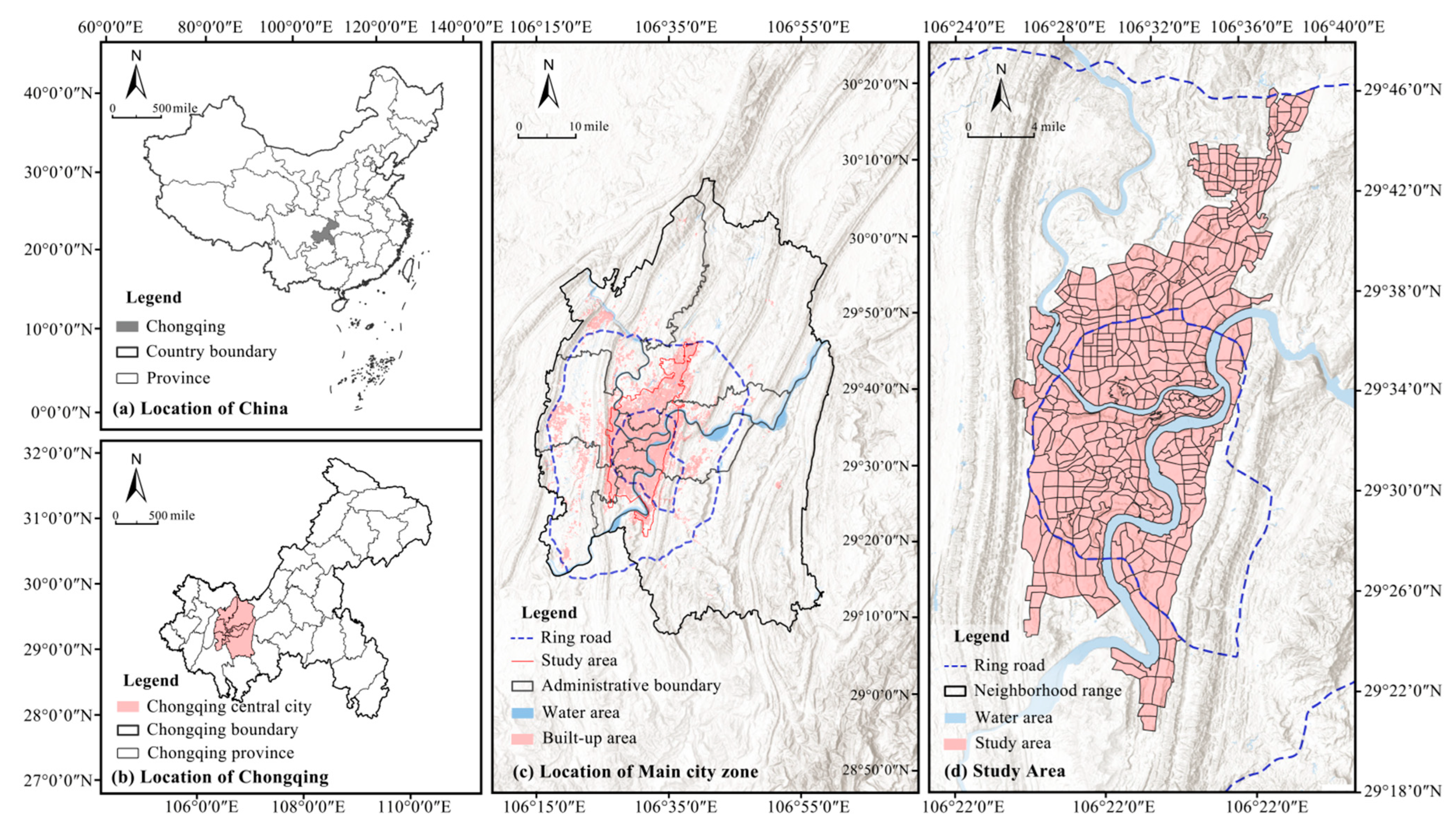
This study measures UV during different time periods (weekdays, weekends, and holidays) using multi-source big data and calculates the BE indicators for each block. It then conducts a comparative analysis of the spatial distribution characteristics of multi-dimensional block vitality. The GBDT model is used to fit the nonlinear relationship between multi-dimensional block vitality and the BE. Finally, the SHAP method is applied to interpret the results of the GBDT model. The research framework is shown in Figure 1.

3.1. Study Area

This study focuses on the central urban area of Chongqing, defined as the core of the city’s main urban district. It includes parts of the Yuzhong, Jiulongpo, Dadukou, Banan, Nan’an, Jiangbei, and Yubei districts, covering approximately 388.20 km2 (see Figure 2). As a typical mountainous city, Chongqing features complex terrain, with north–south mountain ranges intersected by east–west rivers. The study area lies between the Zhongliang and Tongluo Mountains and is characterized by a hilly landscape. It encompasses one central business district (Jiefangbei) and four sub-centers (Guanyin Bridge, Nanping, Shapingba, and Yangjiaping). As the economic, cultural, and population hub of the city, this area exhibits significant variations in UV, making it an ideal subject for analysis.
To better capture the spatial heterogeneity within the city, this study employs a block-level analysis. The block scale provides a more precise reflection of UV differences across neighborhoods and their complex interactions with BE indicators. Based on the methods of Lv et al. [39] and Zhang et al. [53], this paper uses blocks as the basic unit of analysis. In mountainous cities like Chongqing, blocks are particularly suitable for capturing UV because their boundaries align with topographic constraints and human activity patterns. By integrating remote sensing imagery and OpenStreetMap (OSM) road network data, the study area is divided into 418 block units (see Figure 2d). These blocks are divided based on the road network, with block boundaries typically following the natural topographic features of the mountainous city and connecting to areas of high human activity density.

3.2. Data

3.2.1. Urban Vitality

This paper uses heatmap data from the Baidu Map Open Platform (Baidu Heatmap API, https://lbsyun.baidu.com/index.php?title=webapi/heatmap, accessed on 5 November 2024) to measure UV based on the spatial distribution of human activity. Previous research has validated this approach [22]. The data are derived from anonymous user location information collected by the Baidu Map LBS platform, using multi-source positioning technologies (GPS, Wi-Fi, and cell towers) to generate dynamic crowd density distributions. To assess the UV of the study area, this paper selects Baidu heatmap data from typical weekdays, weekends, and holidays between April and October 2024. The data cover 33 days with clear or mostly cloudy weather, including 12 weekdays, 12 weekends, and 9 holidays. For each date type, UV for each time period (morning, afternoon, and evening) is represented by the average heatmap values at four time points (Table 1). Data processing was performed using the zonal statistics tool in ArcGIS Pro 3.0.2 software to calculate crowd density for each block, thereby determining the UV level for each block. Higher crowd density corresponds to stronger UV and vice versa. By calculating the average heatmap values for the selected dates, the average UV levels for each block were determined for weekdays, weekends, and holidays.

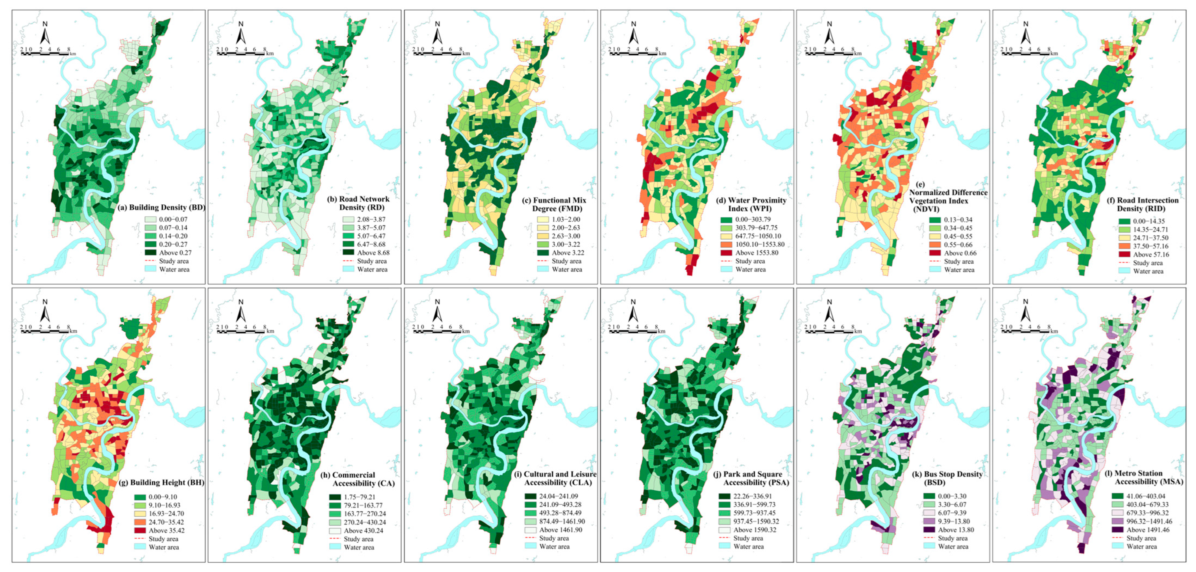
3.2.2. Built Environment

Based on existing research and the specific conditions of the study area, this paper constructs a BE indicator system consisting of 12 indicators across 5 dimensions: density, diversity, design, destination accessibility, and distance to transition. Details of each indicator are provided in Table 2.
The BE data used in this paper include road network data, POI facility data, building vector data, NDVI data, water system data, and bus and subway data. The road network data were sourced from OpenStreetMap (https://www.openstreetmap.org, accessed on 3 December 2024) and processed with topological checks to obtain the road network information for the study area. POI facility data come from the Amap Open Platform (https://ditu.gaode.com/, accessed on 5 December 2024), including attributes such as place names, types, addresses, coordinates, and administrative districts. Building vector data, also sourced from the Amap Open Platform, cover attributes such as the number of floors and the area and perimeter for each building. NDVI data were sourced from the Geographic Remote Sensing Ecological Network (http://www.gisrs.cn/minindex.html, accessed on 20 December 2024), using remote sensing images with a spatial resolution of 30 m to analyze urban green space distribution and environmental quality. Water system data, sourced from OpenStreetMap, provide spatial distribution information of the city’s main water systems, including rivers, lakes, and reservoirs. Finally, bus and subway data, also sourced from the Amap Open Platform, provide information on bus and subway stations within the study area. Using the data above, various built environment indicators were calculated, and their spatial distribution at the block scale is illustrated in Figure 3.

3.3. Methods

This paper uses the GBDT model to explore the nonlinear relationship between UV and the BE and applies the SHAP algorithm to enhance model interpretability.
The GBDT model is suitable for high-dimensional problems with concentrated data feature distributions. It generally outperforms algorithms like support vector machines and random forests, particularly in small sample predictions. Unlike traditional regression models, GBDT learns to adjust the weights of independent variables, fitting the nonlinear relationship between the dependent and independent variables to improve prediction accuracy [54]. Additionally, GBDT is highly tolerant to multicollinearity, outliers, and missing values [55].
GBDT employs an additive model and a forward boosting algorithm, which improves accuracy by combining multiple decision trees. The model typically uses squared error as its loss function and optimizes by fitting residuals. In this study, different models are constructed for the morning, afternoon, and evening periods on weekdays, weekends, and holidays. The data are randomly split into training and testing sets in an 80:20 ratio, and the GradientBoostingRegressor model in the scikit-learn python package (version 1.6.0) is used for fitting. To optimize model performance, 5-fold cross-validation is applied, with a learning rate set to 0.02 and the maximum depth set to 6, ensuring convergence accuracy and capturing nonlinear relationships. The number of decision trees is automatically determined through a hyperparameter optimization process based on the characteristics of each time period. For example, weekday mornings use 292 decision trees, weekend afternoons 283, and holiday evenings 283. These adjustments help optimize model performance based on time period characteristics, resulting in strong resistance to overfitting.
Although the GBDT model excels in accuracy and generalization, its interpretability is limited, making it a “black box” model [45]. To address this, the SHAP algorithm is used to interpret machine learning model outcomes [48]. This study uses SHAP to quantify the contribution of each BE indicator to UV prediction and analyze the impact and importance of each indicator in the model. SHAP interaction effect analysis is also applied to examine the interactive effects of different BE indicator combinations on UV.

4. Results

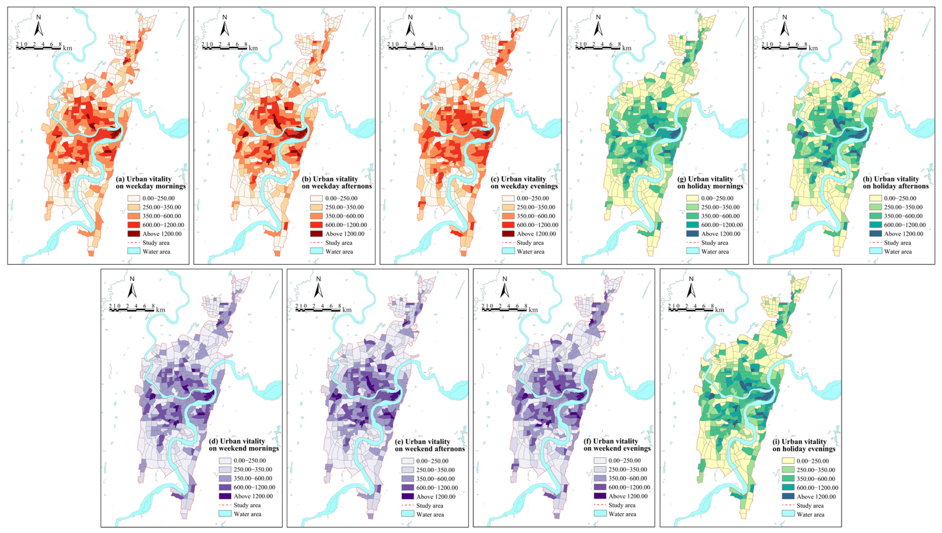
4.1. Spatiotemporal Patterns of Urban Vitality

Figure 4 illustrates the spatial distribution of UV across different time periods on weekdays, weekends, and holidays. Overall, significant differences in UV distribution are observed between the inner and outer ring road areas. Using the Inner Ring Expressway of Chongqing as a boundary, UV in the inner ring area is higher and more concentrated, particularly around commercial and transportation hubs such as Jiefangbei, Guanyin Bridge, Yangjiaping, Nanping, and Shapingba. Notably, the area around Jiefangbei shows the highest UV intensity. These high-vitality areas are supported by natural water systems like the Jialing River and Yangtze River, creating a highly concentrated UV pattern. In contrast, UV outside the inner ring is lower, but several secondary vitality clusters have formed, resulting in a “multi-center, cluster-style” spatial structure. This spatial pattern aligns with the concept of polycentric urban structures, which have been shown to effectively distribute urban activities and resources across multiple sub-centers, thereby enhancing urban vitality and sustainability [56].
On weekdays, the average UV intensity in the study area is 446.09 persons/km2, with 438.93 persons/km2 in the morning, 438.46 persons/km2 in the afternoon, and 460.88 persons/km2 in the evening. This indicates higher UV in the evening, especially around Jiefangbei and Guanyin Bridge. In the evening (Figure 4c), UV extends into outer residential areas, indicating a greater dispersion of activities during nighttime on weekdays. On weekends, UV is slightly higher than on weekdays, averaging 455.62 persons/km2, with the highest intensity in the afternoon (464.66 persons/km2, Figure 4d). This indicates that activities are more concentrated during weekend afternoons. UV on holidays is significantly lower than on weekdays and weekends, with an average intensity of 428.64 persons/km2. Morning UV on holidays (395.11 persons/km2, Figure 4g) is much lower than in the afternoon (441.05 persons/km2, Figure 4h) and evening (458.44 persons/km2, Figure 4i). This may reflect a lower level of activity in the morning on holidays, with UV gradually increasing in the afternoon and evening. Overall, these results highlight the clear spatiotemporal variation in UV within the study area.

4.2. Relative Importance of Built Environment

The R2 values of the GBDT model for the test set are as follows: for weekdays, weekends, and holidays, the R2 values range from 0.8069 to 0.9746, indicating that the model fits well and has a high explanatory power.
This section analyzes the relative importance of BE indicators on UV across different time periods on weekdays, weekends, and holidays using SHAP values, providing a comparative analysis. SHAP values reveal the impact of each BE feature on the model output and illustrate how their importance varies across time periods.
Overall, the sum of the average SHAP values for the BE indicators on weekdays, weekends, and holidays are 491.47, 569.94, and 579.53, respectively. This indicates that the BE has a stronger impact on UV during holidays, which aligns with the findings of Wu et al. (2019) that “urban vitality was more susceptible to the built environment during nonworking times” [57]. In terms of specific time periods, on weekdays and holidays, the evening period has the strongest influence on UV, with holiday evenings having a higher impact than other periods. On weekends, the afternoon period has the greatest impact on UV.
The influence of the BE dimension on UV is ranked in the following order: diversity, design, destination accessibility, density, and distance to transition. Density and destination accessibility have a stronger impact on UV in the afternoon on weekends, while diversity has the most significant impact in the evening. Design has the strongest impact on UV in the evening on holidays, and distance to transition has a stronger impact in the afternoon on holidays. Regarding specific indicators (Figure 5), RID has the greatest impact on UV on weekdays and holidays. BD has the greatest impact on weekend mornings, CLA on weekend afternoons, and CA is most significant on weekend evenings.
As shown in Figure 6, within the density dimension, BD has a greater impact on UV than RD across all time periods, indicating that areas with higher BD are more likely to stimulate UV. The diversity dimension includes only the FMD indicator, which has the strongest impact on UV in the evening on weekends. In the design dimension, RID shows the greatest impact on UV. The impact of other indicators varies significantly across time periods. NDVI has a suppressive effect on UV, while BH and WPI have an enhancing effect. In the destination accessibility dimension, CA and CLA have a greater impact across all time periods, significantly outperforming PSA. The improvement of PSA has both suppressive and enhancing effects on UV. In the distance to transition dimension, MSA has a greater impact on UV than BSD on weekdays and weekends, while BSD is more significant on holidays.

4.3. Nonlinear Impacts of Built Environment on Urban Vitality

4.3.1. Nonlinear Impacts of Density on Urban Vitality

Figure 7 illustrates the nonlinear impacts of BD (Figure 7A) and RD (Figure 7B) on UV across different time periods on weekdays, weekends, and holidays.
It can be observed that both BD and RD have a positive impact on UV when BD exceeds 0.22 and RD reaches 6.39 km/km2, respectively. However, the influence of BD on UV exhibits a pattern of initially increasing and then decreasing, except for holiday mornings. This finding supports Xie et al. (2020) [58], who suggest that higher building density promotes urban vitality. In contrast, RD shows a continuously increasing positive effect on UV. Notably, the critical values of BD and RD at which they positively impact UV are significantly higher during the mornings of weekends and holidays compared to afternoons and evenings. This may be because weekend and holiday mornings have higher activity and traffic, so increasing building and road density boosts UV more effectively. In the afternoons and evenings, activity is lower, so the demand for high building and road density decreases.

4.3.2. Nonlinear Impacts of Diversity on Urban Vitality

As shown in Figure 8, when FMD approaches 3.00, it begins to have a significant positive impact on UV, with the influence continuing to rise, except for the morning on holidays. This indicates that a higher FMD can more effectively enhance UV. In Figure 8g, the critical value at which FMD positively impacts UV during holiday mornings is 3.52, which is higher than in other time periods. The influence increases first, decreases, and rises again. This pattern suggests that the relationship between FMD and UV is likely the result of multi-level, multi-factor interactions. On holiday mornings, UV enhancement is not only influenced by the FMD but also by factors such as specific holiday activities, social interaction patterns, and changes in public demand.

4.3.3. Nonlinear Impacts of Design on Urban Vitality

Figure 9 illustrates the nonlinear impacts of four design factors, WPI (Figure 9A), NDVI (Figure 9B), RID (Figure 9C), and BH (Figure 9D), on UV across different time periods on weekdays, weekends, and holidays.
Firstly, in the afternoon and evening on weekdays and holidays, WPI shows a clear nonlinear impact on UV, divided into four distinct intervals: (1) when WPI is below 277.93 m, it negatively impacts UV, indicating that an excessively low WPI leads to insufficient UV; (2) when WPI is between 277.93 and 400.00 m, it has a positive impact on UV, except for weekday afternoons; (3) when WPI is between 400.00 and 1000.00 m, it negatively impacts UV, suggesting that an excessively high WPI may suppress vitality; (4) when WPI exceeds 1000.00 m, the impact turns positive again, enhancing UV. This change may result from a richer hydrophilic environment, which is associated with more green spaces and water bodies. These elements can enhance the city’s sustainability and ecological appeal, creating environments that foster higher levels of human activity, which in turn boosts UV.
For greenery coverage (Figure 9B), when NDVI is below 0.39, it has a positive impact on UV, but once it exceeds this value, the impact turns negative and stabilizes. This suggests that excessive greening can limit the commercial use of urban spaces and hinder human activity, thereby suppressing the concentration of UV. This trade-off between ecological space and socio-economic vitality echoes the spatial response patterns of ecosystem services observed in urban agglomerations [59]. Nevertheless, this negative effect may be related to the ecological spatial boundary effects and insufficient spatial permeability caused by Chongqing’s complex mountainous terrain. Due to the intricate topography, green spaces are often unevenly distributed and fragmented, potentially forming ecological isolation zones that physically and functionally separate urban spaces, limiting social interaction and mobility. Specifically, in the afternoon on holidays (Figure 9Bh), when NDVI reaches 0.70, it positively impacts UV again. This indicates that higher NDVI during holidays provides more recreational space and comfort, thereby promoting UV.
Road intersection density (Figure 9C) shows that when RID exceeds 41.24 per km2, it positively impacts UV, with the influence gradually increasing. This suggests that a higher RID significantly promotes UV enhancement. The impact of BH (Figure 9D) on UV shows an initial increase, followed by a gradual decline. When BH reaches 23.50 m, UV begins to increase positively, indicating that taller buildings can enhance the spatial perception of an area, thereby fostering the growth of UV. However, excessively tall buildings may lead to negative effects such as spatial congestion and shadowing, which could limit further improvements in UV.

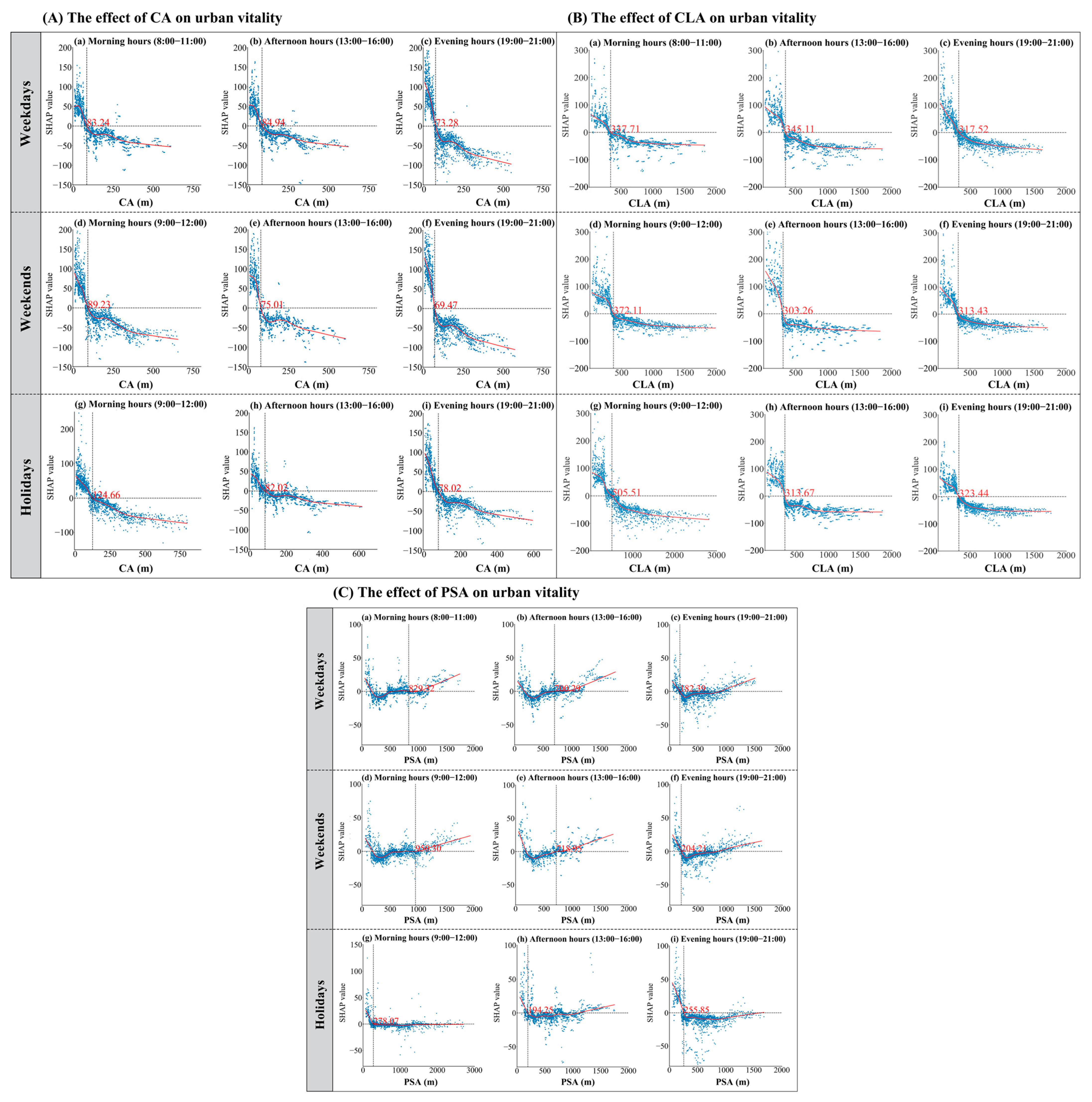
4.3.4. Nonlinear Impacts of Destination Accessibility on Urban Vitality

Figure 10 illustrates the nonlinear impacts of CA (Figure 10A), CLA (Figure 10B), and PSA (Figure 10C) on UV within the dimension of destination accessibility.
The analyses in Figure 10A,B reveal similar trends in the effects of CA and CLA on UV across different time periods. When the distance to the commercial center is below 69.47 m, and the distance to cultural and leisure areas is below 303.26 m, CA and CLA positively influence UV. Beyond these thresholds, their effects turn negative. On holiday mornings, the critical value at which CA (Figure 10Ag) and CLA (Figure 10Bg) negatively impact on UV is higher than in other time periods. This indicates that on holiday mornings, people have a larger activity radius, and the influence of commercial areas extends further, accommodating a wider range of activity demands.
As shown in Figure 10C, when the distance to parks and squares is below 182.39 m, PSA positively impacts UV, indicating that within this range, parks and squares significantly enhance the vitality of the surrounding areas. Between 182.39 m and 950.30 m, the impact turns negative, indicating that the vitality effect of parks and squares gradually weakens as the distance increases. Beyond 950.30 m, the impact turns positive again, suggesting that at longer distances, the attraction of unique parks or green spaces may positively influence UV. Moreover, on holidays and weekends, the critical value at which PSA negatively impacts on UV is higher than on weekdays. This indicates that parks and squares have a broader impact range on UV during these times, accommodating longer activity demands and adapting to the travel patterns of different groups.

4.3.5. Nonlinear Impacts of Distance to Transition on Urban Vitality

Figure 11 illustrates the nonlinear impacts of BSD (Figure 11A) and MSA (Figure 11B) on UV across different time periods during weekdays, weekends, and holidays.
BSD and MSA exhibit opposite trends in their impacts on UV. BSD positively influences UV when reaching 6.15 per/km2, suggesting that higher BSD effectively enhances UV and increases urban mobility. However, MSA shows a positive impact on UV within 618.19 m of a metro station. Beyond this distance, the impact turns negative and eventually stabilizes. This indicates that areas close to metro stations, due to improved accessibility, attract more foot traffic and commercial activities, thereby enhancing UV.

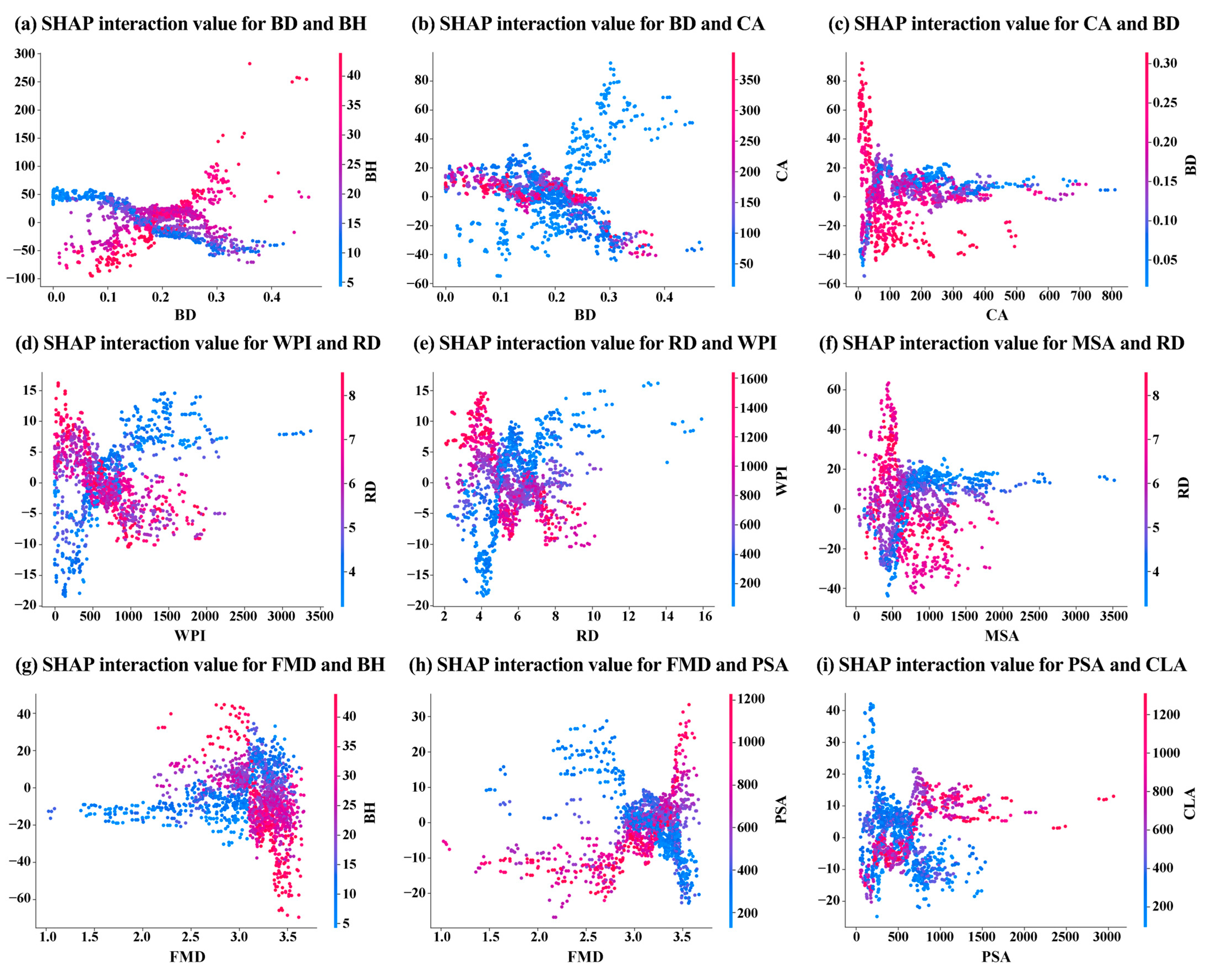
4.4. The Interactive Impacts of Built Environment on Urban Vitality

To further explore the interactive impacts of BE indicators on UV, this study calculates the average UV for weekdays, weekends, and holidays and analyzes the interactions between BE indicators using SHAP values. Nine significant pairs of interactions between BE indicators are selected for analysis, as shown in Figure 12. The X-axis represents the BE indicators, the color axis indicates the other indicator with the strongest interaction effect, and the Y-axis shows the SHAP interaction effect value between the two indicators. A SHAP value greater than 0 indicates a positive interaction effect, while a negative value indicates a negative interaction effect. The larger the SHAP value, the stronger the interaction effect and its impact on UV.
Figure 12a shows that when both BD and BH are high in a block, a positive interaction effect occurs. However, when BD is high and BH is low, the interaction effect becomes negative. Especially when BD is less than 0.18, the increase in BH weakens the positive interaction effect on UV and may even turn it negative. Figure 12b shows that when BD is high and near commercial facilities, a significant positive interaction effect is observed. As BD increases, UV gradually rises. Figure 12c confirms this trend, showing that the critical point for the positive interaction effect between BD and CA is 90 m, with a stronger effect within this distance.
Figure 12d,e illustrate the interaction effects between WPI and RD. When a block is close to water systems and has a high RD, a positive interaction effect occurs. However, beyond 500 m from the water systems, lower road network density actually enhances UV. The critical value for low RD is 5; when RD exceeds this value, the impact of water systems on UV gradually diminishes. Figure 12f further shows that blocks near metro stations with high RD experience a significant increase in UV. As the distance to the metro station increases, the impact of RD gradually weakens and may even turn negative. This indicates that when metro stations are located farther away, the interaction between RD and MSA weakens, reducing its positive impact on UV.
Figure 12g shows that when FMD is less than 3.3 and BH is high, a positive interaction effect occurs. This may be because higher BH improves spatial efficiency and activity clustering in areas with low functional mix, thereby enhancing UV. Figure 12h shows that blocks with a high FMD and a considerable distance from parks and squares exhibit a significant positive interaction effect. However, when FMD is high and the block is near a park or square, the interaction effect turns negative. This may result from spatial conflicts and over-concentration caused by overly dense functional setups and proximity to parks and squares, limiting UV enhancement.
Finally, Figure 12i reveals that when a block is near both parks and squares, as well as cultural and leisure facilities, UV is significantly enhanced. As the distance from parks and squares increases, the interaction effect gradually weakens and may even turn negative. However, when a block is more than 600 m away from parks and squares and also distant from cultural and leisure facilities, the interaction effect turns positive again. This could be because residents begin to rely on other types of social and recreational venues, creating new sources of vitality.

5. Discussion

5.1. Advantages of the Methodology

Although significant progress has been made in studying the nonlinear relationship between the built environment and urban vitality, few studies have explored this relationship at the block scale during weekdays, weekends, and holidays at different times (morning, afternoon, and evening). This paper addresses these gaps through a systematic investigation.
At the theoretical level, this paper employs the GBDT-SHAP model, effectively addressing the issues of underfitting and limited explanatory power that often arise in traditional linear models when dealing with the high-dimensional, complex urban system [60,61]. Additionally, this research fills the gap in understanding the spatiotemporal vitality characteristics and nonlinear mechanisms of mountainous cities [12]. By incorporating factors such as RID and MSA, it provides an in-depth analysis of the nonlinear mechanisms of block-level vitality in the central urban area of Chongqing and compares these findings with the threshold effects observed in flat cities. Chongqing, as a typical mega-mountainous city, features complex terrain that leads to a highly vertical distribution of urban development, with limited connectivity between urban clusters. This paper on Chongqing’s central urban area helps to enrich the geographical diversity of urban vitality research and provides a case study for urban governance in the Chengdu–Chongqing economic circle and the western region.
In terms of analytical scale, most existing studies use regular grid units [31], but this approach struggles to accurately match the boundaries of residents’ actual activities. In contrast, this paper conducts the analysis at the block scale, which better aligns with the spatial logic and human activity range, thereby enhancing the practical applicability and operability of the results.
Furthermore, although most studies have quantified urban vitality from a spatial dimension [33,62], they often overlook its spatiotemporal characteristics. Some studies have distinguished between weekdays and weekends [24,63,64] but have not considered holidays or the detailed variations in daily activities. This paper uses a dual classification method of “characteristic days + time periods” to systematically reveal the dynamic characteristics of urban vitality across different temporal dimensions, significantly enhancing the timeliness and explanatory power of urban vitality measurement.

5.2. Impacts of Single Indicators on Urban Vitality

5.2.1. Spatial Impacts of Built Environment Indicators on Urban Vitality

This study reveals significant differences in the mechanisms through which built environment indicators affect urban vitality between mountainous and flat cities. By comparing with flat cities, we found that the built environment indicators in mountainous cities exhibit more complex nonlinear effects. This paper summarizes the nonlinear thresholds, effect directions, and unique spatial characteristics of these indicators in mountainous cities, as summarized in Table 3 below.
This study reveals significant differences in the mechanisms through which the built environment affects urban vitality in mountainous cities compared to flat cities. For instance, the complex terrain of Chongqing, a typical mega-mountainous city, leads to highly vertical urban development and limited connectivity between urban clusters. This complexity amplifies the threshold effects of density (e.g., RID) and accessibility (e.g., MSA). For example, the critical value for the positive effect of RID on urban vitality in Chongqing is 41.24 per/km2, much higher than in Beijing [65] and Nanjing [66]. This difference stems from the inherent fragmentation of road networks in mountainous cities, which requires higher RID to establish effective connectivity.
Additionally, FMD on urban vitality is more significant in mountainous cities. In Chongqing, higher functional diversity contributes more to urban vitality due to its polycentric urban structure, where the diversity of activities in multiple urban centers promotes mobility and social interaction. This contrasts with cities like Shenzhen, where high-density areas with more monofunctional land use limit the positive impact of functional diversity on vitality [20].
The impact of water systems and green spaces on urban vitality also differs between mountainous and flat cities. In mountainous cities, overly concentrated water bodies can limit available space and reduce environmental permeability. The spatial isolation inherent to mountainous areas means that water bodies and urban spaces do not integrate well, potentially leading to ecological isolation. In contrast, flat cities, with their more uniform topography, allow better integration of water systems with other urban functions, thereby enhancing vitality [67]. In Chongqing, areas near water bodies do not always enhance urban vitality because these spaces are often constrained by the terrain, limiting their integration with other functional areas.
PSA exhibits a first positive, and then negative, and finally positive trend in mountainous cities. Compared to flat cities, mountainous cities have complex terrain, high population density, and compact urban structures [68]. These factors contribute to lower living comfort, leading residents to favor outdoor activities. Consequently, small pocket parks are an ideal solution for utilizing green space in these areas [69]. In flat cities, however, due to the flat terrain and more uniform urban layout, the impact of parks and squares on urban vitality generally decreases monotonically or stabilizes, with less of a positive rebound at long distances. This is mainly because the layout and accessibility of public green spaces in flat cities are better, and the spatial patterns of residents’ activity radii differ from those in mountainous cities.
When analyzing green spaces using NDVI data, the 30 m resolution used in this study may not be sufficient to capture block-scale green space variation in mountainous terrain. The unique terrain characteristics in mountainous cities significantly influence the distribution of green spaces, which often exhibit different spatial patterns compared to flat cities. In particular, green space variation in complex terrain areas tends to be uneven, leading to significantly different patterns of spatial utilization in mountainous cities compared to flat cities. This feature provides a new perspective for understanding the role of green spaces in enhancing urban vitality in mountainous cities.

5.2.2. Temporal Impacts of Built Environment Indicators on Urban Vitality

Based on the characteristics of the temporal dimension, this study further explores how people’s behavioral patterns and spatial demands at different times influence the nonlinear variations in urban vitality. Specifically, in mountainous cities, the complex terrain and limited transportation infrastructure not only affect spatial accessibility but also lead to varying demands for the built environment across different time periods. The activity patterns on weekdays, weekends, and holidays reflect distinct behavioral logics.
On weekdays, people’s main activities focus on daily commuting and commercial engagements, which typically require higher density and good transportation accessibility. Consequently, urban vitality significantly increases with the improvement of indicators such as BD and RD, especially during morning and afternoon periods. When these indicators reach certain thresholds, urban vitality exhibits a strong positive impact during these times. This is consistent with the findings of Fan et al. (2021) [70].
In contrast, activity patterns differ on weekends and holidays. During these periods, people tend to have broader activity ranges, with leisure, social, and tourism-related activities occupying a larger share. Chongqing, as a typical polycentric city, contains multiple functionally distinct tourism and recreational areas that attract large numbers of visitors and residents during holidays, leading to a more dispersed spatial distribution of activities rather than concentration in core high-density zones. Non-commuting diverse activities dominate holiday travel demand, with residents preferring lower-density, greener, and leisure-rich areas, thereby reducing reliance on high-density and high-accessibility zones. Consequently, urban vitality during holidays is more spatially dispersed and typically peaks in the morning. This morning peak mainly results from people’s tendency to schedule outdoor leisure and tourism activities earlier in the day to avoid afternoon heat or evening fatigue. This behavioral pattern, combined with diversified spatial use, interacts to deepen the understanding of spatiotemporal vitality changes in mountainous cities.

5.3. Interaction Effects of Indicators on Urban Vitality

In addition to individual variables, the interaction between built environment indicators also significantly impacts on urban vitality. Through SHAP interaction analysis, this paper identified several key variable combinations, revealing the nonlinear coupling characteristics and spatial complexity between these indicators.
In spatial design, the interaction effects of density variables are particularly crucial. Research indicates a clear synergistic relationship between BD and BH, where high-density and high-rise buildings combine to form vertically integrated spatial types that promote the efficient mixed use of vertical space, thereby significantly enhancing urban vitality [8,27,38]. In mountainous cities, high-density and high-rise structures effectively overcome the horizontal space limitations imposed by terrain, improving land-use efficiency. This effect is especially prominent during peak periods in the morning and evening on weekdays and weekends. However, during holidays, due to changes in people’s activity patterns, recreational, social, and tourism activities tend to be distributed across wider areas, reducing reliance on high-density zones, which weakens the contribution of density and height to urban vitality.
The core of this impact mechanism lies in the ability of high-density and high-rise structures to optimize vertical space utilization, enhance accessibility, and facilitate the integration of functions. This promotes the concentration and flow of human activities, thereby increasing urban vitality. During peak periods on weekdays and weekends, the concentration of activities makes the positive impact of high-density and high-rise structures more significant, particularly during the morning and evening rush hours when commercial and commuting activities are frequent. In contrast, on holidays, the dispersion of activities reduces the attractiveness of dense areas, weakening the role of density and height in promoting vitality. However, when BD is too high and BH is insufficient, spatial congestion and traffic bottlenecks may occur, suppressing urban vitality. Therefore, planners should balance floor area ratio and spatial quality in high-density development in mountainous cities, adjusting space use flexibly according to the varying activity demands at different times and optimizing vertically integrated spaces to maximize their potential to enhance urban vitality.
Moreover, the synergistic effect between density and destination accessibility should not be overlooked. For example, BD shows a significant positive interaction with CA and MSA, meaning that high-density areas with well-developed transportation and service facilities can significantly stimulate human activity [71]. However, if the area is located far from transportation hubs, even with high RD, the reduced transportation efficiency may weaken vitality.
FMD, as a key indicator of block diversity, interacts with other indicators, revealing potential risks of spatial conflicts and usage tensions. For example, when FMD is high and near open spaces like parks and squares, it may suppress urban vitality due to functional overlap or spatial competition. This suggests that urban public space planning should not focus on creating “more and denser” spaces but rather on coordinating and guiding spatial functions.
It is particularly noteworthy that the mixed configuration of different types of public spaces has a strong enhancing effect on urban vitality. For example, when a block is located near both parks and squares as well as cultural and leisure facilities, urban vitality is significantly enhanced. However, if the spatial distribution of such facilities is overly concentrated or their boundaries are unclear, it may lead to resource overlap and functional conflicts. Therefore, careful planning and zoning are essential to optimize these interactions.

5.4. Limitations and Future Research

This study has several limitations and areas for further exploration. Firstly, it is primarily based on a case study of the central urban area of Chongqing, and the generalizability of the results should be further validated in other types of cities. Second, although Baidu heatmap data were used as the primary indicator of urban vitality, they have limitations. These data over-represent smartphone users and exclude groups such as the elderly who may not use smartphones frequently. Additionally, the data collection period (April–October 2024) excludes winter months, which could influence vitality patterns, as some activities and behaviors may vary seasonally. In the future, research could incorporate multi-dimensional indicators such as economic, social, and cultural vitality to create a more comprehensive vitality assessment framework [72]. Furthermore, integrating demographic data from big data platforms, including gender, age, and residential status, could provide insights into the vitality preferences of different population groups. Finally, the perceptual dimension and subjective experience are important aspects that deserve attention [73]. Future research could combine street surveys or street view recognition algorithms to explore the relationship between the built environment and urban vitality from a human perception perspective, driving urban spaces from being merely “usable” to “perceptible, lovable, and sustainable”.

6. Conclusions

This study analyzes 418 blocks in the central urban area of Chongqing, using Baidu heatmap data to analyze the spatiotemporal distribution characteristics of urban vitality across different time periods (morning, afternoon, and evening) on weekdays, weekends, and holidays. The built environment is measured using road network data, POI facility data, building vector data, NDVI data, water system data, and bus and subway data, based on 5 dimensions and 12 indicators. The GBDT model and SHAP explanation method are employed to analyze the nonlinear impacts and interaction effects of the built environment on urban vitality. The following key conclusions are drawn:
(1)
In terms of the spatiotemporal distribution of urban vitality in the central urban area of Chongqing, there are significant differences in urban vitality distribution between the inner and outer ring road areas. The inner ring area shows high and concentrated urban vitality, mainly around commercial and transportation hubs such as Jiefangbei and Guanyin Bridge. In contrast, the outer ring has lower vitality but features several secondary vitality clusters, reflecting a “multi-center, cluster-type” spatial structure. Temporally, urban vitality is higher in the evening on weekdays, stronger in the afternoon on weekends, and generally lower on holidays. Notably, urban vitality is particularly low in the morning on holidays, gradually increasing in the afternoon and evening.
(2)
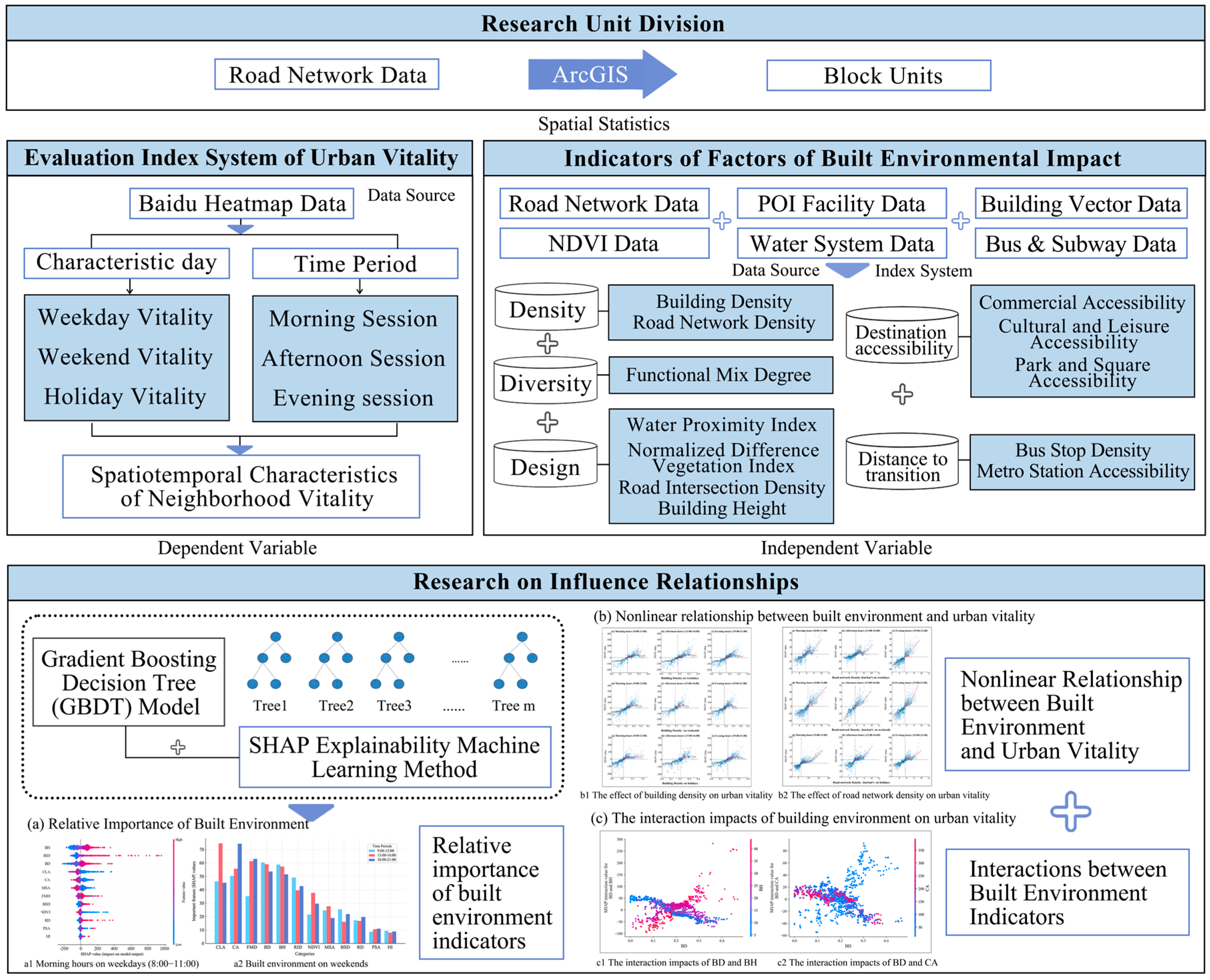
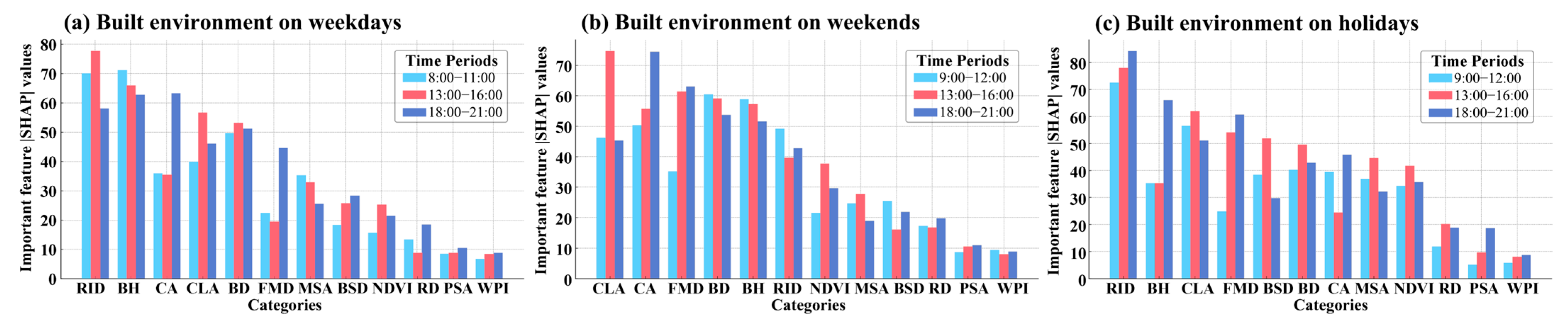
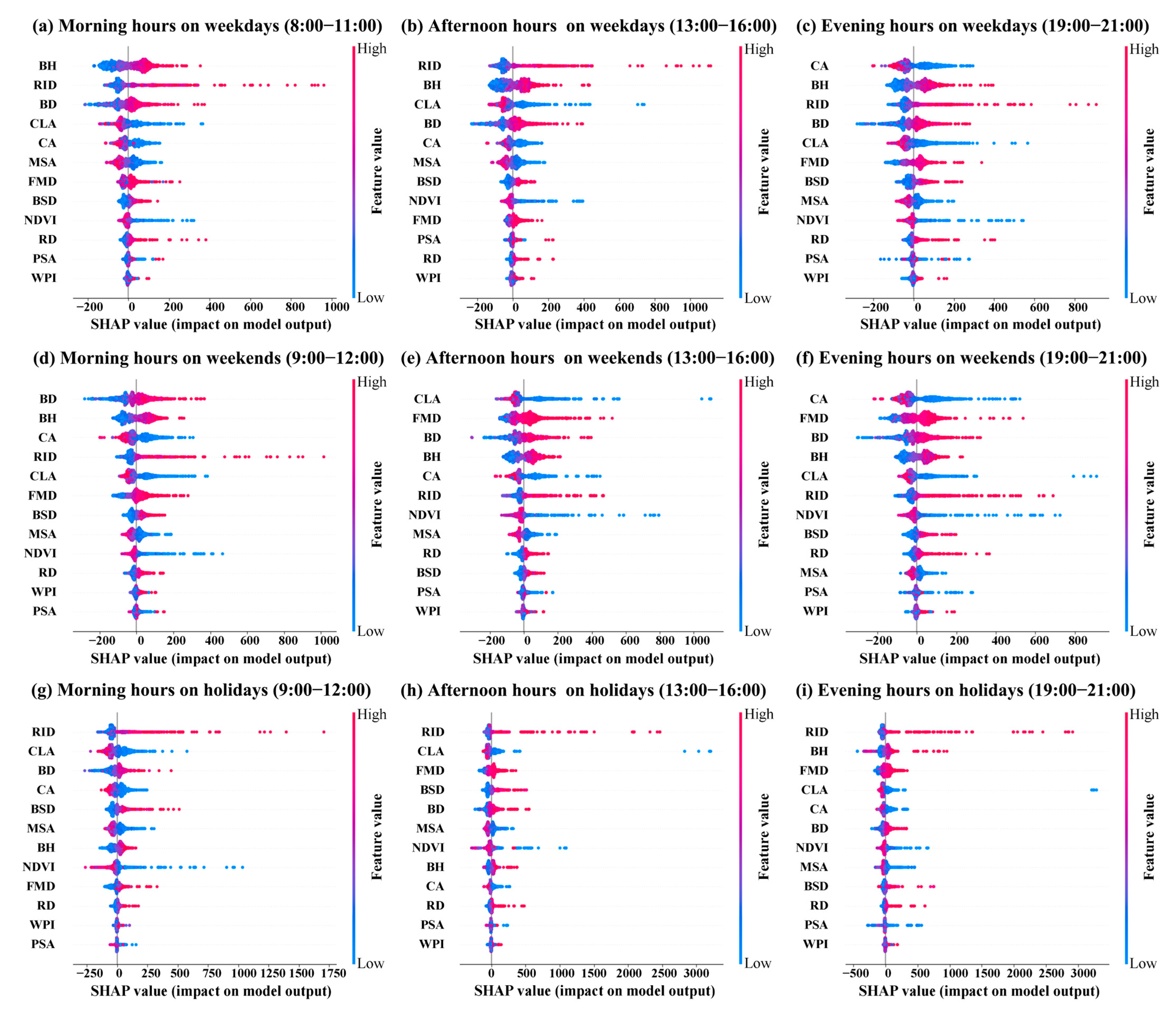
The influence of the built environment’s dimension on urban vitality is ranked in the following order: diversity, design, destination accessibility, density, and distance to transition. The built environment has a stronger overall impact on urban vitality during holidays, with the evening period on holidays having a higher impact than other periods. Specifically, RID has the greatest impact on urban vitality on weekdays and holidays, BD has the greatest impact on the morning of weekends, CLA has the greatest impact on the afternoon of weekends, and CA has the most significant impact on the evening of weekends.
(3)
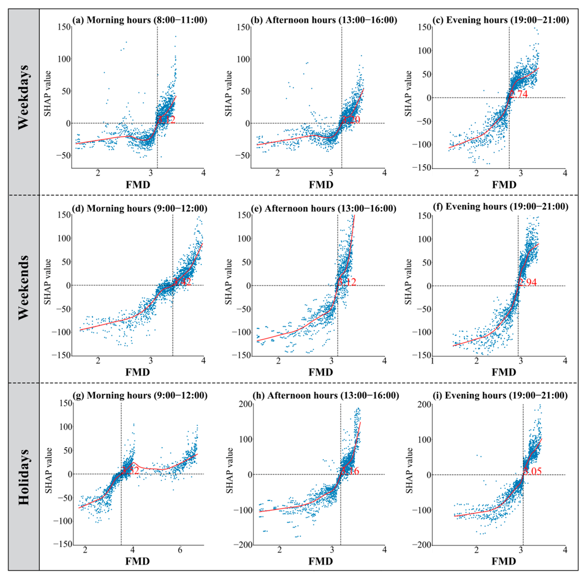
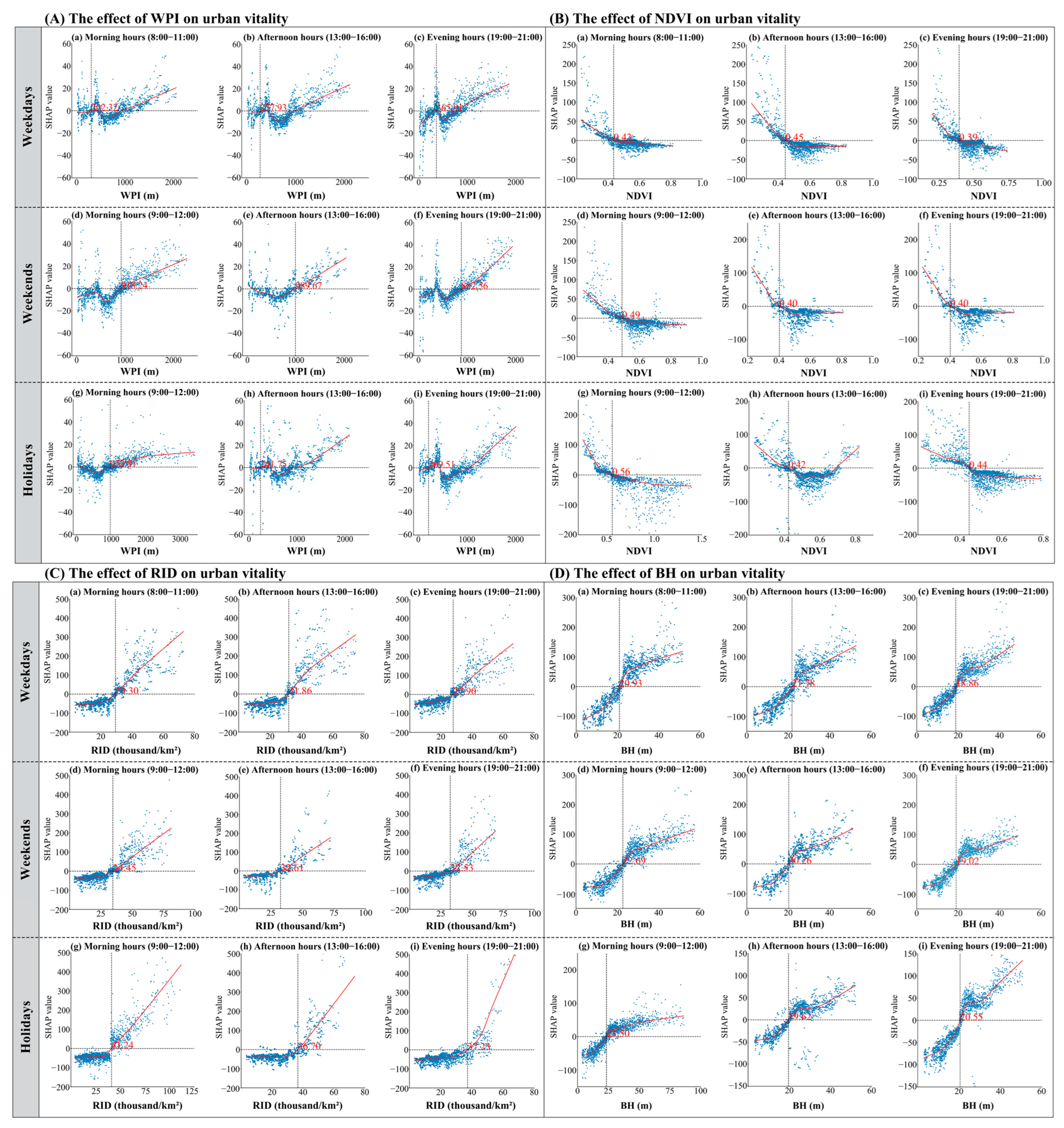
The impacts of the built environment on urban vitality exhibit significant nonlinear characteristics, with BD and PSA showing a first increasing and then inhibiting effect on urban vitality; lower CA, CLA, and MSA have inhibitory effects on urban vitality, with higher NDVI values similarly demonstrating such effects; BH, BSD, RD, and RID have enhancing effects on urban vitality; FMD shows an increase, followed by suppression, and then an increase again in the morning and afternoon on weekdays and in the morning on holidays. In other time periods, it shows an enhancing impact. WPI first shows an inhibiting and then increasing effect on urban vitality in the afternoon on weekends and in the morning on holidays. In other time periods, WPI shows an increase, followed by suppression, and then an increase again.
(4)
There are significant interactive effects among BE indicators such as BD and BH, CA; RD and WPI, MSA; FMD and BH, PSA; PSA and CLA. Considering these interactive relationships comprehensively is of great significance for optimizing BE and enhancing urban vitality.
In mountainous cities, the complex terrain significantly influences the built environment and urban vitality. Chongqing’s highly vertical development and limited connectivity between urban clusters intensify the threshold effects of certain indicators, such as RID and MSA. Compared to flat cities, mountainous cities require higher densities and specific spatial configurations to promote connectivity and vitality. Urban planning in mountainous cities should focus on improving spatial accessibility, optimizing density distribution, and ensuring functional diversity aligns with unique terrain characteristics. Additionally, priority should be given to establishing small green spaces such as pocket parks and recreational areas to balance outdoor activity needs and spatial accessibility. These strategies will support the sustainable development of urban vitality and effectively address the unique challenges of mountainous environments.

Author Contributions

Conceptualization, Jiayu Yang and Enxu Wang; methodology, Jiayu Yang and Enxu Wang; software, Jiayu Yang; validation, Jiayu Yang and Enxu Wang; formal analysis, Jiayu Yang; resources, Enxu Wang; data curation, Jiayu Yang; writing—original draft preparation, Jiayu Yang; writing—review and editing, Jiayu Yang and Enxu Wang; visualization, Jiayu Yang; supervision, Enxu Wang; project administration, Enxu Wang; funding acquisition, Enxu Wang. All authors have read and agreed to the published version of the manuscript.

Funding

This research was funded by the Basic Scientific Research Foundation of the Educational Department of Liaoning Province (JYTMS20230627), the Opening Fund of Liaoning Key Laboratory of Urban and Architectural Digital Technology (UADT2024A02), and the 18th Batch of Innovative Training Program for Undergraduate at Northeastern University (241343).

Data Availability Statement

The data that support the findings of this study are available from the corresponding author, Enxu Wang, upon reasonable request.

Conflicts of Interest

The authors declare no conflicts of interest.

Abbreviations

The following abbreviations are used in this manuscript:
BEBuilt environment
UVUrban vitality
BDBuilding density
RDRoad network density
FMDFunctional mix degree
WPIWater proximity index
NDVINormalized difference vegetation index
RIDRoad intersection density
BHBuilding height
CACommercial accessibility
CLACultural and leisure accessibility
PSAPark and square accessibility
BSDBus stop density
MSAMetro station accessibility

References

  1. Sung, H.; Lee, S.; Cheon, S. Operationalizing Jane Jacobs’s Urban Design Theory: Empirical Verification from the Great City of Seoul, Republic of Korea. J. Plan. Educ. Res. 2015, 35, 117–130. [Google Scholar] [CrossRef]
  2. Lopes, M.N.; Camanho, A.S. Public Green Space Use and Consequences on Urban Vitality: An Assessment of European Cities. Soc. Indic. Res. 2013, 113, 751–767. [Google Scholar] [CrossRef]
  3. Tang, L.; Lin, Y.; Li, S.; Li, S.; Li, J.; Ren, F.; Wu, C. Exploring the Influence of Urban Form on Urban Vibrancy in Shenzhen Based on Mobile Phone Data. Sustainability 2018, 10, 4565. [Google Scholar] [CrossRef]
  4. Sulis, P.; Manley, E.; Zhong, C.; Batty, M. Using mobility data as proxy for measuring urban vitality. J. Spat. Inf. Sci. 2018, 16, 137–162. [Google Scholar] [CrossRef]
  5. Li, M.; Liu, J.; Lin, Y.; Xiao, L.; Zhou, J. Revitalizing historic districts: Identifying built environment predictors for street vibrancy based on urban sensor data. Cities 2021, 117, 103305. [Google Scholar] [CrossRef]
  6. Tang, S.; Ta, N. How the built environment affects the spatiotemporal pattern of urban vitality: A comparison among different urban functional areas. Comput. Urban Sci. 2022, 2, 39. [Google Scholar] [CrossRef]
  7. Kang, C.D. Effects of the human and built environment on neighborhood vitality: Evidence from Seoul, Korea, using mobile phone data. J. Urban Plan. Dev. 2020, 146, 05020024. [Google Scholar] [CrossRef]
  8. Jacobs, J. The Death and Life of Great American Cities; Random House: New York, NY, USA, 1961. [Google Scholar]
  9. Lynch, K. A Theory of Good City Form; MIT Press: Cambridge, MA, USA, 1981. [Google Scholar]
  10. Montgomery, J. Making a city: Urbanity, vitality and urban design. J. Urban Des. 1998, 3, 93–116. [Google Scholar] [CrossRef]
  11. Balram, S.; Dragićević, S. Attitudes toward urban green spaces: Integrating questionnaire survey and collaborative GIS techniques to improve attitude measurements. Landsc. Urban Plan. 2005, 71, 147–162. [Google Scholar] [CrossRef]
  12. Sheng, J.; He, Y.; Lu, T.; Wang, F.; Huang, Y.; Leng, B.; Chen, Y. Unveiling urban vitality and its interactions in mountainous cities: A human behaviour perspective on community-level dynamics. Cities 2025, 159, 105780. [Google Scholar] [CrossRef]
  13. Li, J.; Li, J.; Yuan, Y. Spatiotemporal distribution characteristics and mechanism analysis of urban population density: A case of Xi’an, Shaanxi, China. Cities 2019, 86, 62–70. [Google Scholar] [CrossRef]
  14. Zheng, Q.; Deng, J.; Jiang, R.; Wang, K.; Xue, X.; Lin, Y.; Huang, Z.; Shen, Z.; Li, J.; Shahtahmassebi, A.R. Monitoring and assessing “ghost cities” in Northeast China from the view of nighttime light remote sensing data. Habitat Int. 2017, 70, 34–42. [Google Scholar] [CrossRef]
  15. Zhang, J. Nighttime Vitality and Its Relationship to Urban Diversity: An Exploratory Analysis in Shenzhen, China. IEEE J. Sel. Top. Appl. Earth Obs. Remote Sens. 2022, 15, 309–322. [Google Scholar] [CrossRef]
  16. Weishan, C.; Lin, L.; Yutian, L. Retail center recognition and spatial aggregating feature analysis of retail formats in Guangzhou based on POI data. Geogr. Res. 2016, 35, 703–716. [Google Scholar]
  17. Yue, Y.; Zhuang, Y.; Yeh, A.G.O.; Xie, J.Y.; Ma, C.L.; Li, Q.Q. Measurements of POI-based mixed use and their relationships with neighbourhood vibrancy. Int. J. Geogr. Inf. Sci. 2017, 31, 658–675. [Google Scholar] [CrossRef]
  18. Lu, S.; Shi, C.; Yang, X. Impacts of Built Environment on Urban Vitality: Regression Analyses of Beijing and Chengdu, China. Int. J. Environ. Res. Public Health 2019, 16, 4592. [Google Scholar] [CrossRef]
  19. Wu, C.; Ye, X.; Ren, F.; Du, Q. Check-in behaviour and spatio-temporal vibrancy: An exploratory analysis in Shenzhen, China. Cities 2018, 77, 104–116. [Google Scholar] [CrossRef]
  20. Li, Z.; Zhao, G. Revealing the spatio-temporal heterogeneity of the association between the built environment and urban vitality in Shenzhen. ISPRS Int. J. Geo-Inf. 2023, 12, 433. [Google Scholar] [CrossRef]
  21. Calabrese, F.; Diao, M.; Di Lorenzo, G.; Ferreira, J.; Ratti, C. Understanding individual mobility patterns from urban sensing data: A mobile phone trace example. Transp. Res. Part C Emerg. Technol. 2013, 26, 301–313. [Google Scholar] [CrossRef]
  22. Lyu, G.; Angkawisittpan, N.; Fu, X.; Sonasang, S. Enhancing urban vitality through big data: A case study of Yinchuan City using GWR and GBDT models. Sci. Rep. 2023, 15, 579. [Google Scholar]
  23. Wu, Y.; Xie, C.; Zhang, A.; Zhao, T.; Cao, J. Spatiotemporal analysis of urban vitality and its drivers from a human mobility perspective. ISPRS Int. J. Geo-Inf. 2025, 14, 167. [Google Scholar]
  24. Chen, Y.; Yu, B.; Shu, B.; Yang, L.; Wang, R. Exploring the spatiotemporal patterns and correlates of urban vitality: Temporal and spatial heterogeneity. Sustain. Cities Soc. 2023, 91, 104440. [Google Scholar] [CrossRef]
  25. Wu, C.; Ye, Y.; Gao, F.; Ye, X. Using street view images to examine the association between human perceptions of locale and urban vitality in Shenzhen, China. Sustain. Cities Soc. 2023, 88, 104291. [Google Scholar] [CrossRef]
  26. Duan, J.; Wang, H.; Liu, L.; Zhang, J. The attraction gradient of urban functions: How does functional mix at multiple scales predict urban vitality. Cities 2025, 156, 105516. [Google Scholar] [CrossRef]
  27. Lin, J.; Zhuang, Y.; Zhao, Y.; Li, H.; He, X.; Lu, S. Measuring the non-linear relationship between three-dimensional built environment and urban vitality based on a random forest model. Int. J. Environ. Res. Public Health 2023, 20, 734. [Google Scholar] [CrossRef]
  28. Cervero, R.; Kockelman, K. Travel demand and the 3Ds: Density, diversity, and design. Transp. Res. Part D Transp. Environ. 1997, 2, 265–294. [Google Scholar] [CrossRef]
  29. Ewing, R.; Cervero, R. Travel and the built environment: A meta-analysis. J. Am. Plan. Assoc. 2010, 76, 265–294. [Google Scholar] [CrossRef]
  30. Wu, W.; Ma, Z.; Guo, J.; Niu, X.; Zhao, K. Evaluating the effects of built environment on street vitality at the city level: An empirical research based on spatial panel durbin model. Int. J. Environ. Res. Public Health 2022, 19, 1664. [Google Scholar] [CrossRef]
  31. Chen, L.; Zhao, L.; Xiao, Y.; Lu, Y. Investigating the spatiotemporal pattern between the built environment and urban vibrancy using big data in Shenzhen, China. Comput. Environ. Urban. Syst. 2022, 95, 101827. [Google Scholar] [CrossRef]
  32. Xia, C.; Yeh, A.G.O.; Zhang, A. Analyzing spatial relationships between urban land use intensity and urban vitality at street block level: A case study of five Chinese megacities. Landsc. Urban Plan. 2020, 193, 103669. [Google Scholar] [CrossRef]
  33. Chen, S.; Lang, W.; Li, X. Evaluating urban vitality based on geospatial big data in Xiamen Island, China. Sage Open 2022, 12, 21582440221134519. [Google Scholar] [CrossRef]
  34. Wan, J.; Xie, Q.; Fan, X. The impact of transportation and information infrastructure on urban productivity: Evidence from 256 cities in China. Struct. Change Econ. Dyn. 2024, 68, 384–392. [Google Scholar] [CrossRef]
  35. Fuentes, L.; Miralles-Guasch, C.; Truffello, R.; Delclòs-Alió, X.; Flores, M.; Rodríguez, S. Santiago de Chile through the eyes of Jane Jacobs: Analysis of the conditions for urban vitality in a Latin American metropolis. Land 2020, 9, 498. [Google Scholar] [CrossRef]
  36. Zumelzu, A.; Barrientos-Trinanes, M. Analysis of the effects of urban form on neighborhood vitality: Five cases in Valdivia, Southern Chile. J. Hous. Built Environ. 2019, 34, 897–925. [Google Scholar] [CrossRef]
  37. Sallis, F.J.; Cerin, E.; Conway, L.T.; Adams, A.M.; Frank, D.L.; Pratt, M. Physical activity in relation to urban environments in 14 cities worldwide: A cross-sectional study. Lancet 2016, 387, 2207–2217. [Google Scholar] [CrossRef]
  38. Huang, B.; Zhou, Y.; Li, Z.; Song, Y.; Cai, J.; Tu, W. Evaluating and characterizing urban vibrancy using spatial big data: Shanghai as a case study. Environ. Plan. B Urban Anal. City Sci. 2020, 47, 1543–1559. [Google Scholar] [CrossRef]
  39. Lv, G.; Zheng, S.; Hu, W. Exploring the relationship between the built environment and block vitality based on multi-source big data: An analysis in Shenzhen, China. Geomat. Nat. Hazards Risk 2022, 13, 1593–1613. [Google Scholar] [CrossRef]
  40. Huang, J.; Hu, X.; Wang, J.; Lu, A. How diversity and accessibility affect street vitality in historic districts? Land 2023, 12, 219. [Google Scholar] [CrossRef]
  41. Huang, B.; Wu, B.; Barry, M. Geographically and temporally weighted regression for modeling spatio-temporal variation in house prices. Int. J. Geogr. Inf. Sci. 2010, 24, 383–401. [Google Scholar] [CrossRef]
  42. Yang, J.; Cao, J.; Zhou, Y. Elaborating non-linear associations and synergies of subway access and land uses with urban vitality in Shenzhen. Transp. Res. Part A Policy Pract. 2021, 144, 74–88. [Google Scholar] [CrossRef]
  43. Ding, C.; Cao, X.J.; Næss, P. Applying gradient boosting decision trees to examine non-linear effects of the built environment on driving distance in Oslo. Transp. Res. Part A Policy Pract. 2018, 110, 107–117. [Google Scholar] [CrossRef]
  44. Yang, L.; Ao, Y.; Ke, J.; Lu, Y.; Liang, Y. To walk or not to walk? Examining non-linear effects of streetscape greenery on walking propensity of older adults. J. Transp. Geogr. 2021, 94, 103099. [Google Scholar] [CrossRef]
  45. Song, Y.; Zhang, S.; Deng, W. Nonlinear hierarchical effects of housing prices and built environment based on multiscale life Circle-A case study of Chengdu. ISPRS Int. J. Geo-Inf. 2023, 12, 371. [Google Scholar] [CrossRef]
  46. Liu, D.; Lu, Y.; Yang, L. Exploring non-linear effects of environmental factors on the volume of pedestrians of different ages using street view images and computer vision technology. Travel Behav. Soc. 2024, 36, 100814. [Google Scholar] [CrossRef]
  47. Zhang, Y.; Haghani, A. A gradient boosting method to improve travel time prediction. Transp. Res. Part C Emerg. Technol. 2015, 58, 308–324. [Google Scholar] [CrossRef]
  48. Ling, Z.; Zheng, X.; Chen, Y.; Qian, Q.; Zheng, Z.; Meng, X.; Shi, X. The nonlinear relationship and synergistic effects between built environment and urban vitality at the neighborhood scale: A case study of Guangzhou’s central urban area. Remote Sens. 2024, 16, 2826. [Google Scholar] [CrossRef]
  49. Gao, F.; Deng, X.; Liao, S.; Liu, Y.; Li, H.; Li, G.; Chen, W. Portraying business district vibrancy with mobile phone data and optimal parameters-based geographical detector model. Sustain. Cities Soc. 2023, 96, 104635. [Google Scholar] [CrossRef]
  50. Yang, W. The nonlinear effects of multi-scale built environments on CO2 emissions from commuting. Transp. Res. Part D Transp. Environ. 2023, 118, 103736. [Google Scholar] [CrossRef]
  51. Zhao, L.; Zhang, M.; Cheng, S.; Fang, Y.; Wang, S.; Zhou, C. Investigate the effects of urban land use on PM2.5 concentration: An application of deep learning simulation. Build. Environ. 2023, 242, 110521. [Google Scholar] [CrossRef]
  52. Ma, J.; Cheng, J.C.; Jiang, F.; Chen, W.; Zhang, J. Analyzing driving factors of land values in urban scale based on big data and non-linear machine learning techniques. Land Use Policy 2020, 94, 104537. [Google Scholar] [CrossRef]
  53. Zhang, Z.; Liu, J.; Wang, C.; Zhao, Y.; Zhao, X.; Li, P.; Sha, D. A spatial projection pursuit model for identifying comprehensive urban vitality on blocks using multisource geospatial data. Sustain. Cities Soc. 2024, 100, 104998. [Google Scholar] [CrossRef]
  54. Liu, J.; Wang, B.; Xiao, L. Non-linear associations between built environment and active travel for working and shopping: An extreme gradient boosting approach. J. Transp. Geogr. 2021, 92, 103034. [Google Scholar] [CrossRef]
  55. Ding, H.; Zhao, Z.; Wang, S.; Zhang, Y.; Zheng, X.; Lu, X. Quantifying the impact of built environment on traffic congestion: A nonlinear analysis and optimization strategy for sustainable urban planning. Sustain. Cities Soc. 2025, 122, 106249. [Google Scholar] [CrossRef]
  56. Yu, H.; Yang, J.; Li, T.; Jin, Y.; Sun, D. Morphological and functional polycentric structure assessment of megacity: An integrated approach with spatial distribution and interaction. Sustain. Cities Soc. 2022, 80, 103800. [Google Scholar] [CrossRef]
  57. Wu, W.; Niu, X. Influence of built environment on urban vitality: Case study of Shanghai using mobile phone location data. J. Urban Plan. Dev. 2019, 145, 04019007. [Google Scholar] [CrossRef]
  58. Xie, Y.; Shang, C.; Deng, X. Evolution of urban vitality drivers from 2014 to 2022: A case study of Kunming, China. Int. J. Environ. Sci. Technol. 2025, 1–14. [Google Scholar] [CrossRef]
  59. Yu, H.; Yang, J.; Sun, D.; Li, T.; Liu, Y. Spatial Responses of Ecosystem Service Value during the Development of Urban Agglomerations. Land 2022, 11, 165. [Google Scholar] [CrossRef]
  60. Zhang, Z.; Zhao, L.; Zhang, M. Exploring non-linear urban vibrancy dynamics in emerging new towns: A case study of the Wuhan metropolitan area. Sustain. Cities Soc. 2024, 112, 105580. [Google Scholar] [CrossRef]
  61. Tao, T.; Cao, J. Exploring nonlinear and collective influences of regional and local built environment characteristics on travel distances by mode. J. Transp. Geogr. 2023, 109, 103599. [Google Scholar] [CrossRef]
  62. Huang, X.; Jiang, P.; Li, M.; Zhao, X. Applicable Framework for Evaluating Urban Vitality with Multiple-Source Data: Empirical Research of the Pearl River Delta Urban Agglomeration Using BPNN. Land 2022, 11, 1901. [Google Scholar] [CrossRef]
  63. Xia, X.; Zhang, Y.; Zhang, Y.; Rao, T. The spatial pattern and influence mechanism of urban vitality: A case study of Changsha, China. Front. Environ. Sci. 2022, 10, 942577. [Google Scholar] [CrossRef]
  64. Zhao, K.; Guo, J.; Ma, Z.; Wu, W. Exploring the spatiotemporal heterogeneity and stationarity in the relationship between street vitality and built environment. Sage Open 2023, 13, 21582440231152226. [Google Scholar] [CrossRef]
  65. Jin, A.; Ge, Y.; Zhang, S. Spatial Characteristics of Multidimensional Urban Vitality and Its Impact Mechanisms by the Built Environment. Land 2024, 13, 991. [Google Scholar] [CrossRef]
  66. Yang, L.; Wu, M.; Chen, Y.; Wu, C. Examining the impact of the urban transportation system on tangible and intangible vitality at the city-block scale in Nanjing, China. Environ. Plan. B Urban Anal. City Sci. 2024, 51, 1833–1853. [Google Scholar] [CrossRef]
  67. Zhang, S.; Lu, J.; Guo, R.; Yang, Y. Exploring the Relationship Between Visual Perception of the Urban Riverfront Core Landscape Area and the Vitality of Riverfront Road: A Case Study of Guangzhou. Land 2024, 13, 2142. [Google Scholar] [CrossRef]
  68. Li, H.; Xie, H. Noise exposure of the residential areas close to urban expressways in a high-rise mountainous city. Environ. Plan. B Urban Anal. City Sci. 2021, 48, 1414–1429. [Google Scholar] [CrossRef]
  69. Dong, J.; Guo, R.A.; Guo, F.; Guo, X.M.; Zhang, Z. Pocket parks–a systematic literature review. Environ. Res. Lett. 2023, 18, 167. [Google Scholar] [CrossRef]
  70. Fan, Z.; Duan, J.; Luo, M.; Zhan, H.; Liu, M.; Peng, W. How did built environment affect urban vitality in urban waterfronts? A case study in Nanjing reach of Yangtze River. ISPRS Int. J. Geo-Inf. 2021, 10, 611. [Google Scholar] [CrossRef]
  71. Zhang, Y.; Wang, X.; Wang, L.; Li, G.; Zhang, Y.; Ye, Y.; Song, J. Measurement and optimization of sustainable urban form elements in New Urban districts using multi-source data. Front. Environ. Sci. 2024, 12, 1451903. [Google Scholar] [CrossRef]
  72. Jalaladdini, S.; Oktay, D. Urban public spaces and vitality: A socio-spatial analysis in the streets of Cypriot towns. Procedia Soc. Behav. Sci. 2012, 35, 664–674. [Google Scholar] [CrossRef]
  73. Mouratidis, K.; Poortinga, W. Built environment, urban vitality and social cohesion: Do vibrant neighborhoods foster strong communities? Landsc. Urban Plan. 2020, 204, 103951. [Google Scholar] [CrossRef]
Figure 1. Diagram of the technical framework.
Ijgi 14 00225 g001
Figure 2. Location of research area and urban blocks in it.
Ijgi 14 00225 g002
Figure 3. Spatial distribution of built environment indicators at the block scale.
Ijgi 14 00225 g003
Figure 4. Urban vitality on weekdays, weekends, and holidays.
Ijgi 14 00225 g004
Figure 5. Relative importance of independent variables at different periods.
Ijgi 14 00225 g005
Figure 6. Variable importance ranking and contribution based on the SHAP model.
Ijgi 14 00225 g006
Figure 7. The effect of density on urban vitality.
Ijgi 14 00225 g007
Figure 8. The effect of diversity on urban vitality.
Ijgi 14 00225 g008
Figure 9. The effect of design on urban vitality.
Ijgi 14 00225 g009
Figure 10. The effect of destination accessibility on urban vitality.
Ijgi 14 00225 g010
Figure 11. The effect of distance to transition on urban vitality.
Ijgi 14 00225 g011
Figure 12. The interaction impacts of building environment on urban vitality.
Ijgi 14 00225 g012
Table 1. Selected time periods for urban vitality measurement.
Date TypeMorning HoursAfternoon HoursEvening Hours
Weekdays8:00–11:0013:00–16:0018:00–21:00
Weekends9:00–12:0013:00–16:0018:00–21:00
Holidays9:00–12:0013:00–16:0018:00–21:00
Table 2. Built environment indicator based on 5D dimensions.
DimensionIndicatorAbbr.DescriptionData Source
DensityBuilding DensityBDBuilding footprint area/block areaGaode Map.
Road Network Density(km/km2)RDTotal road length inside the block (outward-facing roads)/block areaOSM data.
DiversityFunctional Mix DegreeFMDDiversity index of various POIs within the block (calculated using Shannon’s diversity index)Gaode Map.
DesignWater Proximity Index (m)WPIDistance from block centroid to nearest water bodyOSM data.
Normalized Difference Vegetation IndexNDVIAverage fractional vegetation cover within the blockGisrs.
Road Intersection Density (thousand/km2)RIDNumber of road intersections/block areaOSM data.
Building Height (m)BHAverage building height within the blockGaode Map.
Destination AccessibilityCommercial Accessibility (m)CADistance from block centroid to nearest commercial POIGaode Map.
Cultural and Leisure Accessibility (m)CLADistance from block centroid to nearest cultural and leisure POIGaode Map.
Park and Square Accessibility (m)PSADistance from block centroid to nearest park or squareGaode Map.
Distance to transitionBus Stop Density (thousand/km2)BSDNumber of bus stops inside the block/block areaGaode Map.
Metro Station Accessibility (m)MSADistance from block centroid to nearest metro stationGaode Map.
Table 3. Spatial characteristics of the built environment’s impact on urban vitality in Chongqing.
IndicatorNonlinear ThresholdImpact DirectionMountain City Characteristics
BD0.22First negative and then positiveTerrain limits space compactness, moderate density promotes vitality
RD6.39 km/km2First negative and then positiveDispersed road network requires higher density for accessibility
FMD3.00First negative and then positiveFunctional diversity promotes vitality, adapts to complex terrain
WPI277.93 m, 400.00 m, 1000.00 mFirst negative and then positive and then negative and then positiveWater distribution is limited by terrain; restricted space utilization affects vitality
NDVI0.39First positive and then negativeExcessive greening leads to spatial isolation, reducing social density
RID41.24 per/km2First negative and then positiveDispersed road network, high-density intersections promote traffic connectivity and vitality
BH23.50 mFirst negative and then positiveLarge terrain elevation difference, higher buildings improve spatial perception, but excessive height may cause spatial congestion; moderate increase promotes vitality
CA69.47 mFirst positive and then negativeDue to complex terrain, the influence of commercial areas is limited; too distant commercial areas no longer attract people, leading to decreased vitality
CLA303.26 mFirst positive and then negativeDue to complex terrain, the influence of cultural and recreational areas is limited; too distant areas no longer attract people, leading to decreased vitality
PSA182.39 m, 950.30 mFirst positive and then negative, then positiveGreening concentrated in mountains and slopes, nearby parks have strong attraction, but at greater distances, the attraction gradually decreases due to terrain limitations
BSD6.15 per/km2First negative, then positiveWhen the traffic network density is low in mountainous cities, vitality is limited; as density increases, traffic improves, and vitality increases
MSA618.19 mFirst positive, then negativeWhen metro stations are far, commuting is difficult, and vitality is lower
Disclaimer/Publisher’s Note: The statements, opinions and data contained in all publications are solely those of the individual author(s) and contributor(s) and not of MDPI and/or the editor(s). MDPI and/or the editor(s) disclaim responsibility for any injury to people or property resulting from any ideas, methods, instructions or products referred to in the content.

