Evaluating Spatio-Temporal Kriging with Machine Learning Considering the Sources of Spatio-Temporal Variation

Abstract

Integrating spatio-temporal kriging with machine learning improves estimation accuracy by addressing complex spatial and temporal variations in spatio-temporal phenomena. The improvement can be attributed to the enhanced flexibility of machine learning in capturing non-linear global trends, which traditional methods struggle to model, while kriging remains effective in representing spatio-temporal interactions. However, differences in the estimated global trends and spatio-temporal interactions resulting from applying machine learning may influence the spatio-temporal variation patterns of the kriging results. Therefore, this study evaluates the effectiveness of machine learning in spatio-temporal kriging using NO₂ concentrations in Seoul, focusing on its impact on overall accuracy and the contributions to global trends and spatio-temporal interactions. The results show that integrating machine learning enhances overall accuracy relative to ordinary spatio-temporal kriging. Global trend estimates differ by the models, with polynomial regression producing smoother patterns but larger errors, while random forest and boosting yield more abrupt patterns with smaller errors. These differences lead to smoother kriging outcomes in the polynomial model and more discrete patterns in the ensemble-based models. This study highlights the importance of considering both overall estimation accuracy and spatio-temporal patterns when selecting kriging methods.

1. Introduction

The integration of machine learning techniques and kriging methods improves estimation accuracy [1,2]. Expanding spatio-temporal dimensions increases modeling complexity compared to purely spatial models [3]. Traditionally, polynomial regression or trend surface analysis has been commonly used to remove global variation trends to achieve stationarity in kriging [4]. While traditional methods offer simple and comprehensive estimates, these conventional methods often lack the flexibility to capture complex and non-linear spatial and temporal patterns. In contrast, machine learning techniques effectively address these variations [5]. Accordingly, applying machine learning to spatio-temporal kriging enhances the accuracy of estimating variables, particularly environmental ones such as air pollution, which exhibit complex and non-linear seasonal variations in emission sources [6,7,8,9].

Empirical studies have demonstrated the advantages of integrating kriging with machine learning. For example, Dai et al. (2014) [10] demonstrated that integrating an artificial neural network with kriging led to more accurate predictions of soil organic matter content based on root mean square error (RMSE) and Lin’s concordance correlation coefficient. Similarly, Li et al. (2011) [11] applied machine learning techniques to spatial interpolation of environmental variables and reported improved overall accuracies when combining these methods for mud content interpolation. Shao et al. (2020) [12] also found that integrating random forest with spatio-temporal kriging outperformed random forest without kriging in terms of overall accuracy. These studies have commonly applied machine learning techniques to enhance the accuracy of kriging-based estimation. However, they have primarily focused on improvements in overall accuracy.

Although previous studies have reported that combining kriging with machine learning improves overall accuracy, the individual contributions of each method to estimation accuracy and their influence on the resulting spatio-temporal patterns remain underexplored. Since spatio-temporal variation can be decomposed into first-order effects representing global trends and second-order effects capturing localized interactions [13], relying solely on a combined overall accuracy metric such as RMSE may obscure their individual contributions. This focus on improving overall accuracy has often overlooked the distinct contributions of global trends and spatio-temporal interactions, particularly with spatial pattern preservation. Moreover, each machine learning-based kriging estimates global trends differently, which in turn affects the estimations of localized interactions. Evaluating their accuracy separately is essential for understanding their distinct contributions, which may lead to estimation patterns that differ from those of traditional kriging. In addition, the high flexibility of machine learning enables it to capture abrupt variations [14], which may lead to estimation patterns that differ from those of traditional spatio-temporal kriging. This further highlights the importance of evaluating the accuracy based on individual effects.

This study evaluates the effectiveness of integrating machine learning into spatio-temporal kriging by explicitly decomposing spatio-temporal variation into global trends and spatio-temporal interactions. In particular, it differs from previous studies by assessing the kriging results from the perspective of decomposed spatio-temporal variation rather than relying on overall accuracy metrics. Specifically, this study estimates NO₂ concentrations in Seoul using spatio-temporal kriging integrated with machine learning. Machine learning methods such as random forest, boosting, and polynomial regression are used to estimate global trends, while spatio-temporal kriging is applied to the residuals to estimate spatio-temporal interactions. The resulting estimates are evaluated based on overall accuracy (i.e., RMSE) and the individual contributions of the global trends and spatio-temporal interactions to that accuracy. Furthermore, this study examines the spatial and temporal distribution of these contributions by fixing either the spatial or temporal dimension.

2. Materials and Methods

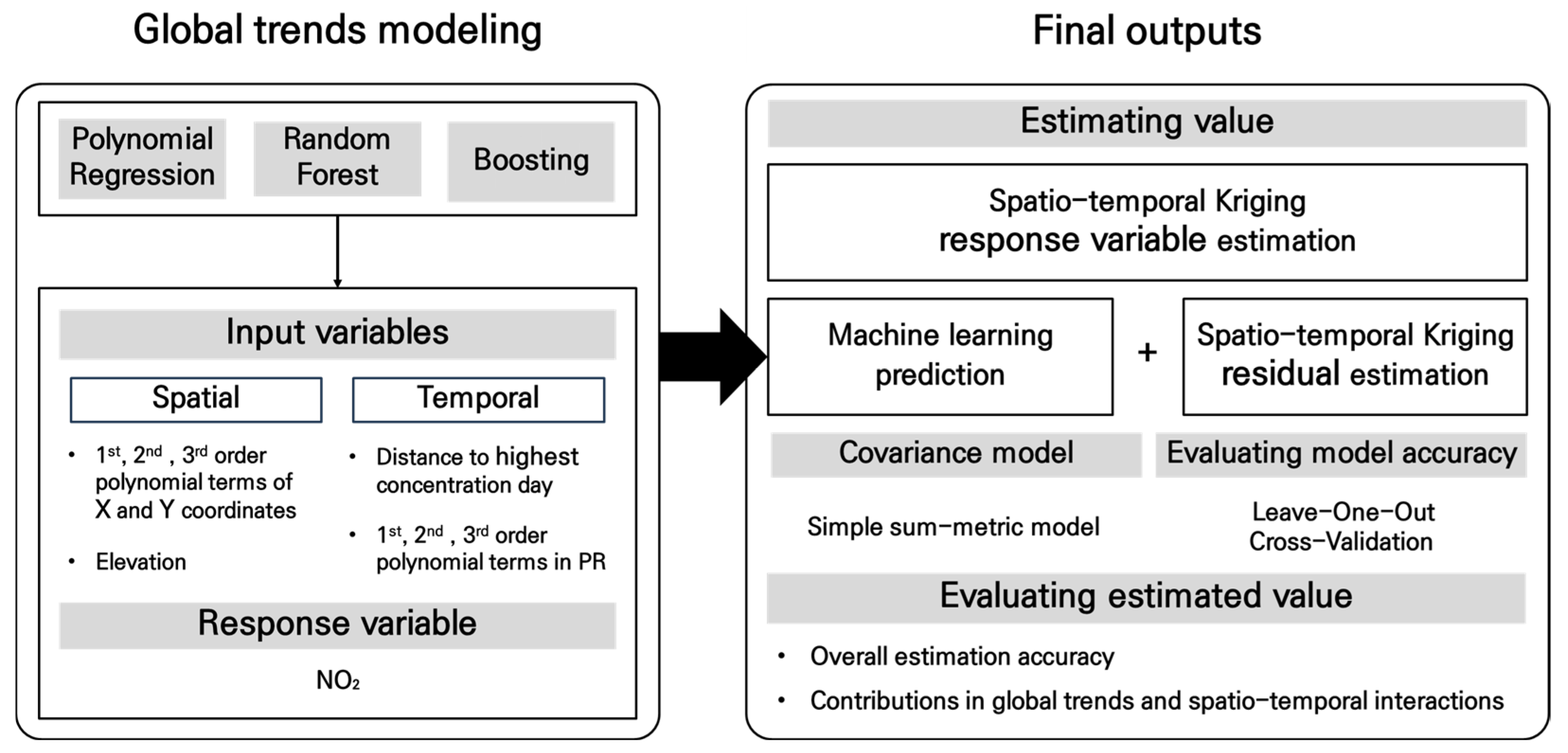
This section outlines the methodological framework of the study to examine the effectiveness of machine learning in estimating NO₂ levels in Seoul using spatio-temporal kriging (Figure 1). First, it introduces the fundamentals of kriging and spatio-temporal kriging, focusing on achieving spatio-temporal stationarity through global trends estimation and applying kriging to residuals to model the spatio-temporal interactions. Next, it outlines the machine learning methods used to estimate the global trends, including the input and response variables and the hyperparameter tuning procedures. The estimation of the spatio-temporal interactions is then described, with emphasis on semivariogram modeling and the specification of the covariance model. This is followed by a description of the evaluation procedure for kriging performance based on the combined effects. Finally, the study area and the target variable for interpolation are introduced.

Kriging is a stochastic interpolation method to predict unknown values at unmeasured locations while minimizing the mean squared error [15], and spatio-temporal kriging is an extension of the spatial kriging method into the spatio-temporal dimension [16]. When predicting air quality measures such as NO₂ levels, spatio-temporal kriging provides more effective estimates than conventional kriging since air quality exhibits strong spatio-temporal dependencies. In other words, considering only the spatial dimension may result in the loss of important information due to spatio-temporal dependency [17] because air quality data generally tends to be correlated with spatially and temporally neighboring observations.

This study estimates the global trends effects using machine learning and applies spatio-temporal kriging to the residuals of the machine learning output to estimate the spatio-temporal interactions. In kriging, observed values at sample points are generally decomposed into three components: the global trend (i.e., first-order effects), the spatio-temporal interactions (i.e., second-order effects), and residuals [13,17,18,19]. Second-order stationarity is a crucial prerequisite for applying kriging, as it assumes a constant mean and a covariance structure that depends solely on relative distances rather than absolute locations. This prerequisite is often achieved by removing the global trends from the observed values, which also serve to classify different kriging methods (e.g., simple, ordinary, and universal kriging) [20].

This study analyzes the estimation of the global trends under varying spatial, temporal, and spatio-temporal conditions using the most widely utilized machine learning techniques, such as polynomial regression, random forest, and boosting [21,22]. Specifically, the response variable in the machine learning models represents NO₂ concentration levels in Seoul from 1 January to 31 December 2023 (refer to Figure 2). The set of input variables is designed to estimate the spatial and temporal variations in global trends. To capture spatial variation, elevation is included, as NO₂ concentrations generally exhibit a decreasing trend with increasing altitude [23]. In addition, third-order polynomial terms of the x- and y-coordinates, which are commonly employed in universal kriging and trend surface analysis, are used to represent spatial structure. Temporal variation is modeled using the number of days elapsed since the annual peak in NO₂ concentration.

The following describes the hyperparameter tuning for the polynomial regression, random forest, and boosting models. Polynomial regression (PR), widely used in conventional universal kriging, provides a simple and interpretable baseline for capturing spatial and temporal trends [24], which utilizes the aforementioned input variables. Random forest (RF) constructs an ensemble of decision trees to improve prediction accuracy. It is based on the Bagging technique, which reduces variance by training each tree on bootstrapped samples [25]. Additionally, RF selects a random subset of input variables at each split to decrease correlations among trees; the number of variables selected at each split is a key hyperparameter influencing model performance, which is tuned using Out-of-Bag (OOB) samples. Boosting (BT) improves prediction accuracy by iteratively fitting the residuals of previous trees, with the learning rate controlling the contribution of each tree to the final model [26]. To ensure stable predictive performance and prevent overfitting, the number of trees is varied from 100 to 5000 in increments of 100, and the interaction depth is set to 3, 4, or 5, with a fixed learning rate of 0.01. Hyperparameters are tuned using 5-fold cross-validation.

To estimate spatio-temporal interactions through spatio-temporal kriging, a variogram is used to quantify and model spatial and temporal autocorrelation. It typically demonstrates an increase in semi-variance with increasing spatio-temporal lag distance and is characterized by three key parameters: nugget, sill, and range. The nugget effect represents the variance observed at zero distance [27]. The range indicates the distance beyond which spatial or temporal autocorrelation becomes negligible, while the sill corresponds to the total variance observed at the range [28].

In spatio-temporal kriging, the covariance model characterizes the dependency structure between observations across both space and time. This study adopts the simple sum-metric covariance model. The sum-metric model integrates spatial, temporal, and spatio-temporal components, allowing for independent spatial and temporal variability while capturing their interactions. The simple sum-metric model is a simplified version of the sum-metric model, in which the spatio-temporal nugget effect is reduced to a single term [29]. The simple sum-metric model variogram is given by the following equation (Equation (1)):

$$\gamma \left(h,u\right)=nug\cdot 1_{h>0\vee u>0}+{\gamma }_{\mathbf{s}}\left(h\right)+{\gamma }_t\left(u\right)+{\gamma }_{joint}\left(\sqrt{h^2+{\left(\kappa \cdot u\right)}^2}\right)$$

(1)

where ${\gamma }_s$, ${\gamma }_t$, and ${\gamma }_{joint}$ denote spatial, temporal, and joint variograms. $\kappa$ is a spatio-temporal anisotropy coefficient between spatial distance $h$ and temporal distance $u$. $\kappa$ was tuned within the range of 40 to 300 [8,29]. Each variogram consists of three parameters $\theta =\{{\tau }^2,{\sigma }^2,\phi \}$: the nugget, partial sill, and range.

The estimated spatio-temporal kriging results are evaluated based on overall estimation accuracy using RMSE, as well as the contributions of the global trends and spatio-temporal interactions to improvements in accuracy. Leave-one-out cross-validation (LOOCV) is employed to evaluate kriging performance by comparing ordinary spatio-temporal kriging (OSTK) with machine learning-based STK methods. In the machine learning-STK approaches, the final estimated value is obtained by combining the machine learning prediction (i.e., global trends estimation) with the interpolated residuals (i.e., spatio-temporal interactions estimation), and RMSE is calculated as the difference between the observed and final estimated values at monitoring stations.

Finally, this section describes the study area and the target variable for interpolation. The target variable is nitrogen dioxide (NO₂) concentration, measured in parts per billion (ppb), derived from hourly air quality data collected by Air Korea sensors [30] and aggregated into daily averages from 1 January to 31 December 2023. The analysis uses data from 40 sensors within Seoul and 31 sensors within 10 km of the city boundary to reduce spatial extrapolation and edge effects (Figure 2a). The training dataset in machine learning consists of both external and internal data, while only internal data was used for kriging evaluation. To capture spatial variation, the machine learning models use first-, second-, and third-order polynomial terms of the x- and y-coordinates and elevation. Temporal variation is represented by the number of days since January 11, the day with the highest NO₂ concentration (Figure 2b). Polynomial regression also incorporates polynomial terms of this temporal variable to capture non-linear temporal trends.

3. Results

This section presents the evaluation results to assess the effectiveness of machine learning in enhancing spatio-temporal kriging. It begins with the variogram results used to model spatial and temporal dependencies. The overall accuracy of the spatio-temporal kriging methods was then assessed. To examine accuracy patterns across space and time, the analysis was conducted by fixing either the spatial or temporal dimension. For temporal variation, a single monitoring station with the highest average NO₂ concentration was selected to evaluate changes in prediction accuracy over time. For spatial variation, the date with the highest observed NO₂ concentration, January 11, was fixed, and differences in spatial prediction accuracy on that day were examined.

First, the semivariogram results are presented to provide an overall understanding of spatial and temporal dependency structures in NO₂ concentrations (

Table 1. Estimated parameters of the variograms.

Parameter	OSTK	PRSTK	RFSTK	BTSTK
$\mathrm{spatial}\mathrm{sill}\left({{\sigma }_{\mathbf{s}}}^2\right)$	$14.86\left({\mathrm{p}\mathrm{p}\mathrm{b}}^2\right)$	$13.88\left({\mathrm{p}\mathrm{p}\mathrm{b}}^2\right)$	$0.43\left({\mathrm{p}\mathrm{p}\mathrm{b}}^2\right)$	$1.00\left({\mathrm{p}\mathrm{p}\mathrm{b}}^2\right)$
$\mathrm{spatial}\mathrm{range}({\phi }_{\mathbf{s}}$)	2602.59 m	2458.70 m	1498.67 m	529.10 m
$\mathrm{temporal}\mathrm{sill}({{\sigma }_t}^2$)	$68.53\left({\mathrm{p}\mathrm{p}\mathrm{b}}^2\right)$	$70.41\left({\mathrm{p}\mathrm{p}\mathrm{b}}^2\right)$	$3.13\left({\mathrm{p}\mathrm{p}\mathrm{b}}^2\right)$	$2.65\left({\mathrm{p}\mathrm{p}\mathrm{b}}^2\right)$
$\mathrm{temporal}\mathrm{range}({\phi }_t$)	1.87 days	1.76 days	0.77 days	1.73 days

and Figure A1 in Appendix A). Specifically, to model the semivariogram, the spatial lag size was set to 1500 m, with a maximum separation distance of 15,000 m, and temporal lags ranged from 0 to 14 days with a lag size of one day. This configuration provides the best fit for the semivariogram model. The RMSE values of the fitted variograms increased in the following order—RFSTK (0.35), BTSTK (0.35), PRSTK (5.98), and OSTK (6.13)—indicating that the semivariogram models are generally appropriately fitted. Moreover, the lower RMSEs observed in the machine learning-based STK methods reflect smaller residuals after applying machine learning.

The semivariogram results generally converge at short spatio-temporal lags, although the patterns vary depending on the spatio-temporal kriging method (Table 1). Because the residuals after removing the global trends are relatively larger, OSTK and PRSTK tend to exhibit higher sills and longer spatio-temporal ranges than RFSTK and BTSTK. Compared to PRSTK, OSTK, which assumes the same global trends across all space and time, shows a higher sill and broader range. Specifically, OSTK yields higher estimates for the spatial (${{\sigma }_{\mathbf{s}}}^2=$14.86 $\left({\mathrm{p}\mathrm{p}\mathrm{b}}^2\right)$) and temporal (${{\sigma }_t}^2=$68.53 $\left({\mathrm{p}\mathrm{p}\mathrm{b}}^2\right)$) sill, as well as the spatial (${\phi }_{\mathbf{s}}=$ 2602.59 m) and temporal (${\phi }_t=$1.87 days) range (Table 1). In contrast, PRSTK shows a relatively lower spatial sill (13.88 $\left({\mathrm{p}\mathrm{p}\mathrm{b}}^2\right)$) but a higher temporal sill (70.41 $\left({\mathrm{p}\mathrm{p}\mathrm{b}}^2\right)$), with slightly shorter spatial (2458.70 m) and temporal (1.76 days) ranges.

In contrast, due to the relatively small residuals after removing the global trends using machine learning, RFSTK and BTSTK demonstrate markedly lower sills and narrower ranges in both spatial and temporal dimensions compared to OSTK and PRSTK (Table 1). Specifically, RFSTK yields notably lower estimates for the spatial (0.43 $\left({\mathrm{p}\mathrm{p}\mathrm{b}}^2\right)$) and temporal (3.13 $\left({\mathrm{p}\mathrm{p}\mathrm{b}}^2\right)$) sills, as well as the spatial (1498.67 m) and temporal (0.77 days) ranges. Similarly, BTSTK reflects localized global trends with small spatial (1.00 $\left({\mathrm{p}\mathrm{p}\mathrm{b}}^2\right)$) and temporal (2.65 $\left({\mathrm{p}\mathrm{p}\mathrm{b}}^2\right)$) sills, and short spatial (529.10 m) and temporal (1.73 days) ranges. Compared to RFSTK, BTSTK shows lower sills in both spatial and temporal dimensions, with a shorter spatial range but a longer temporal range.

The following presents the results for the overall accuracy of the spatio-temporal kriging methods (

Table 2. RMSE of estimations of global trends and spatio-temporal interactions.

RMSE	OSTK	PRSTK	RFSTK	BTSTK
Only global trends	15.26	10.01	2.38	2.81
With spatio-temporal interactions		5.94	2.36	2.60

). The evaluation is based on two types of RMSE: one calculated from the residuals after removing the global trends, and the other after applying spatio-temporal kriging to estimate the spatio-temporal interactions. As suggested by the semivariogram results, the RMSE reduction attributable to global trend estimation is more pronounced in RFSTK and BTSTK, which incorporate machine learning. Specifically, the results show that, in general, OSTK and PRSTK, which are similar to conventional universal kriging, achieve a substantial reduction in RMSE through kriging by estimating spatio-temporal interactions. In contrast, for RFSTK and BTSTK, most of the RMSE reduction is achieved by estimating the global trends through machine learning.

In other words, although RFSTK shows the highest overall predictive accuracy based on the final spatio-temporal kriging RMSE, this performance is largely attributable to the estimation of the global trends. Since the primary objective of kriging lies in estimating spatio-temporal interactions, the limited role of kriging in capturing spatio-temporal variation when combined with machine learning methods raises concerns regarding the methodological justification for its application. Specifically, based on the final spatio-temporal RMSE, RFSTK reports the highest accuracy (2.36), followed by BTSTK (2.60), PRSTK (5.94), and OSTK (15.26). Among the global trends predictions, RF yields the lowest RMSE (2.38), followed by BT (2.81) and PR (10.01), as the ensemble models (RF and BT) effectively capture spatial and temporal variation as part of the global trends. Despite its relatively lower predictive accuracy for the global trends compared to the ensemble models, PRSTK achieves a substantial improvement in spatio-temporal interactions estimation, with an RMSE reduction of 4.07. In contrast, RFSTK and BTSTK show only minimal improvement from kriging, with RMSE reductions of just 0.02 and 0.21, respectively.

The following presents the results of temporal accuracy variation in spatio-temporal kriging (Figure 3). Specifically, to evaluate this, a single monitoring station with the highest average NO₂ concentration is selected, and for visualization, observed NO₂ concentrations (shown in black) and STK-estimated concentrations are averaged over five-day intervals. The STK estimates are further separated into NO₂ concentrations predicted using only the global trends (shown in blue) and those estimated using only the spatio-temporal interactions (shown in yellow).

PRSTK tends to estimate smooth temporal global trends, in contrast to the relatively abrupt patterns observed in RFSTK and BTSTK. At the selected monitoring station, although the observed NO₂ concentrations exhibit local temporal fluctuations, their overall levels tend to be higher in spring and winter and lower in summer and fall. The global trends estimated by PRSTK using polynomial regression (blue bars in Figure 3b) provide a smooth representation of the general seasonal trend. However, it fails to account for local fluctuations, resulting in relatively large residuals on days with elevated NO₂ levels during summer and fall. In contrast, RFSTK and BTSTK effectively capture localized temporal variations rather than general seasonal trends, yielding global trends estimates that appear more abrupt compared to those of PRSTK, while still producing relatively small residuals (blue bars in Figure 3c,d).

The different global trends estimations across kriging methods influence the estimation of spatio-temporal interactions, i.e., the estimation tendency of STK. In other words, because kriging is applied to the residuals after removing the global trends, the trends in global trends estimation directly affect the modeling of spatio-temporal dependencies in the kriging process. PRSTK estimates a smooth representation of the general seasonal global trends, which results in larger residuals. Consequently, a greater portion of the prediction is attributed to the spatio-temporal interactions estimated by STK (yellow bars in Figure 3b), and the modeled semivariogram also indicates relatively higher sills compared to other models.

RFSTK and BTSTK, which model temporally localized global trends, exhibit distinct patterns at the selected station. Specifically, RFSTK tends to underestimate NO₂ concentrations during winter and spring and overestimate them during summer and fall (yellow bars in Figure 3c). As a result, the contribution of the spatio-temporal interactions is generally greater in winter and spring, where residuals are larger. In contrast, BTSTK alternates between overestimation and underestimation across days, leading to corresponding fluctuations in the magnitude of spatio-temporal interaction estimates (yellow bars in Figure 3d). Although both models produce low RMSE values after removing the global trends, resulting in smaller modeled sills, BTSTK shows a relatively larger range than RFSTK, likely reflecting its response to localized temporal variability at the selected station.

Finally, the spatial variations in the STK estimates were examined (Figure 4). To evaluate spatial variation, the date with the highest observed NO₂ concentration, 11 January, was selected. The interpolated values are displayed on a 300 m × 300 m grid for visualization. The STK results are organized into two components: the predicted global trends across the entire study area after modeling them from the observed data (Figure 4c,e,g), and the final interpolation results including both the global trends and spatio-temporal interactions (Figure 4a,b,d,f).

First, an examination of the global trends reveals that, similar to the temporal variation results, PRSTK tends to produce smoother spatial estimations based on visual diagnostics, whereas RFSTK and BTSTK exhibit more abrupt spatial patterns. Specifically, the global trends estimated by PRSTK tend to be generally underestimated and show a smooth spatial trend, with values increasing toward the southeast and in areas of lower elevation (Figure 4c). In contrast, RFSTK and BTSTK display more abrupt spatial patterns than PRSTK, although spatial discrepancies between the two methods are also evident. To facilitate comparison, the classification intervals were kept consistent across the corresponding maps. RFSTK estimates a relatively larger cluster of high NO₂ concentrations in the central–western part (Figure 4e), whereas BTSTK identifies smaller, more localized clusters of elevated values (Figure 4g).

Second, the final interpolation results, which incorporate both global trends and spatio-temporal interactions, also display distinct patterns across STK methods. PRSTK shows a noticeable difference from its global trends-only estimates and maintains a smooth spatial pattern. For comparability, the maps were constructed using consistent classification intervals. Specifically, at the selected date, the global trends in PRSTK appear to be underestimated, and the final prediction is obtained by summing this underestimated trend with the spatio-temporal interactions estimates. The STK component of PRSTK shows a spatial pattern similar to that of OSTK (Figure 4a), which assumes constant global trends across the study area. As a result, clusters of high NO₂ concentrations form around monitoring stations with high global trends estimates (Figure 4b). Because both the global trends and spatio-temporal interactions estimations in PRSTK exhibit smooth spatial trends, the final interpolated surface also reflects this pattern.

BTSTK and RFSTK yield results that are more consistent with their global trends predictions and produce more abrupt patterns compared to PRSTK and OSTK. Specifically, RFSTK and BTSTK account for a substantial portion of the spatial variation through their global trends, resulting in final interpolation outputs that closely resemble their global trend estimations, apart from the presence of moderately expanded clusters of high values. Comparing the two methods, RFSTK produces relatively larger clusters (Figure 4d), likely due to the larger spatial range identified in its semivariogram analysis, while BTSTK maintains more localized clusters (Figure 4f). Both methods, consistent with their global trends estimates, yield abrupt and linear spatial patterns that reflect the inherent structure of tree-based machine learning [31].

4. Conclusions

This study evaluates the effectiveness of integrating machine learning into spatio-temporal kriging by addressing the sources of spatial and temporal variation. First, the analysis results show that the integration improves overall estimation accuracy. In particular, the increased flexibility of machine learning allows for more detailed representations of global trends. However, this detailed representation reduces the portion of variations explained by spatio-temporal interactions based on kriging.

Second, each spatio-temporal kriging method produces distinct spatio-temporal patterns, mainly due to differences in the spatio-temporal patterns of the estimated global trends. Specifically, OSTK, which relies primarily on spatio-temporal interactions, typically yields smooth patterns, and PRSTK exhibits smooth trends in both the global trends and spatio-temporal interactions. However, the results indicate that machine learning models (i.e., RFSTK and BTSTK), particularly tree-based, generate more abrupt spatio-temporal patterns in the global trends and reduce the proportion of variation attributed to spatio-temporal interactions.

The selection of a kriging model should account for not only overall accuracy but also the character of variation in spatio-temporal phenomena. If the variations exhibit smooth and gradual changes over space and time, OSTK and PRSTK are more suitable for capturing these long-range trends. These models are particularly advantageous in applications where preserving overall structural patterns and minimizing abrupt fluctuations are essential, especially in cases of relatively smooth variation that is independent of enumeration units. In contrast, when localized variations are more pronounced and exhibit abrupt changes, RFSTK and BTSTK provide more appropriate estimations for identifying and emphasizing discrete concentration shifts. This makes them especially useful in cases where sudden changes in spatial and temporal data require detailed representation. Distinguishing between smooth and abrupt patterns often relies on data behavior and visual diagnostics [32]. As reported in previous studies [33], NO₂ concentrations typically exhibit smooth variation, a pattern also observed in this study. PRSTK is, therefore, more suitable as it captures gradual differences in both global trends and spatio-temporal interactions, even though its overall accuracy is lower than that of RFSTK and BTSTK.

This study provides two insights into the field of spatio-temporal interpolation. First, overall accuracy may not be a sufficient criterion for selecting a spatio-temporal kriging model. Specifically, it shows that improvements in overall accuracy resulting from the integration of machine learning and kriging are primarily due to the effective capture of global trends. However, a greater emphasis on modeling global trends may diminish the role of kriging in explaining spatio-temporal variation. Second, this study highlights the importance of considering the character of variation in spatio-temporal phenomena when selecting a kriging method. By evaluating the contributions of different sources of variation, the study shows that when the influence of an abrupt global trends estimation is substantial, it can lead to more abrupt overall patterns in the final interpolation results. The proposed method may be especially beneficial in applications where preserving spatial patterns is critical, such as in disease cluster detection [34] or location allocation [35].

This study can be extended in the following ways. First, further evaluation of various machine learning models that can be integrated with kriging is needed. While this study utilizes tree-based machine learning models, ensemble approaches built on other algorithms, e.g., regression-based models, may generate different spatio-temporal patterns. Second, the approach can be extended to other cases that involve different characteristics of variation in spatio-temporal phenomena. In particular, further investigation is needed for phenomena that exhibit more abrupt patterns than the air pollution data used in this study. Third, improving the computational scalability of integrated machine learning and kriging approaches for large-scale datasets remains an important challenge.