

Viewpoint Selection for 3D Scenes in Map Narratives

Abstract
1. Introduction
- (1)
- Introducing spatial distance as a quantitative measure to assess the narrative relevance of elements within a scene.
- (2)
- Proposing a constraint framework to regulate the visual differentiation of elements in narrative processes.
- (3)
- Applying a chaotic particle swarm optimization algorithm to achieve efficient and interpretable viewpoint selection for narrative scenes.
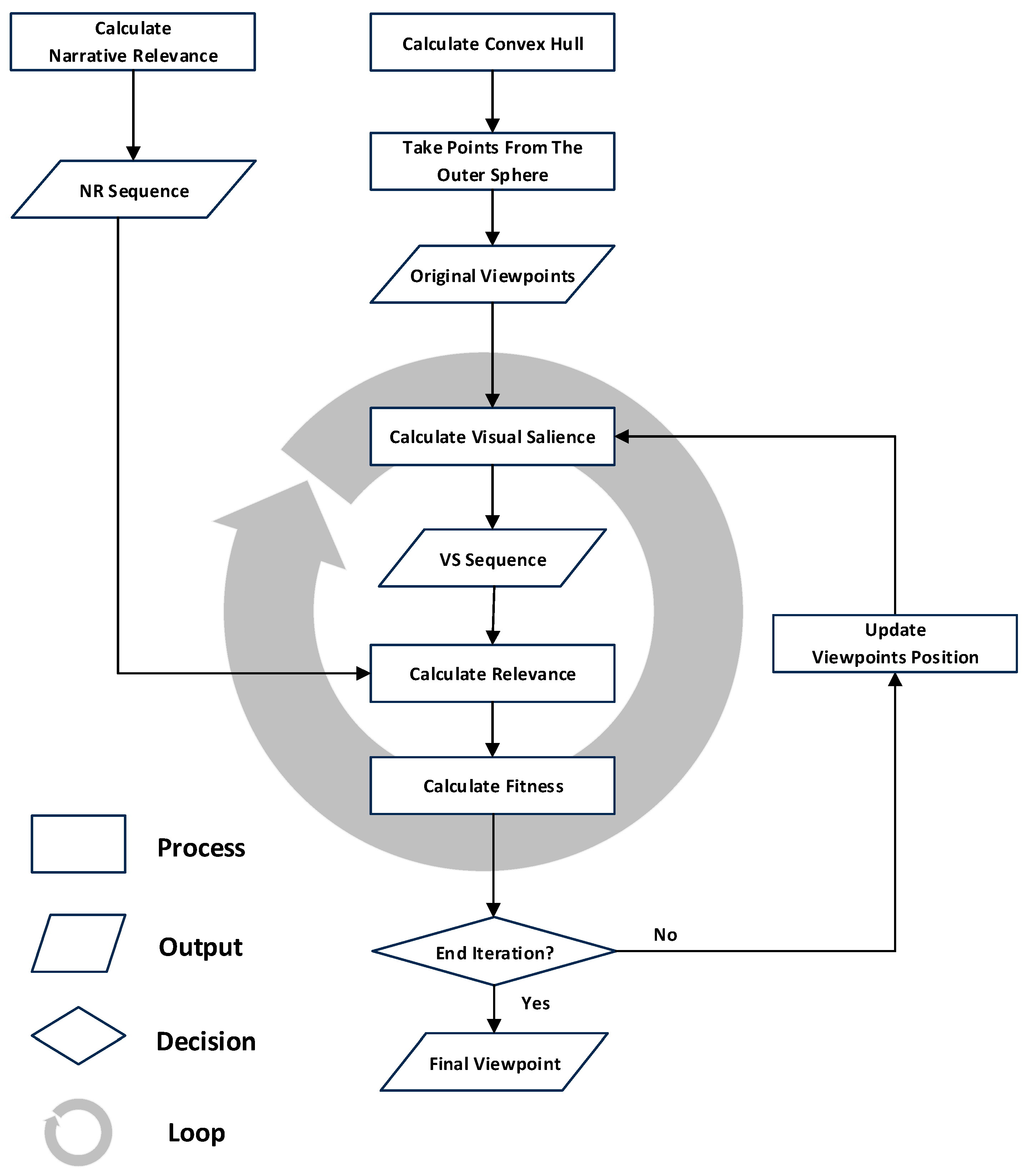
2. Methodological Framework
2.1. Overview
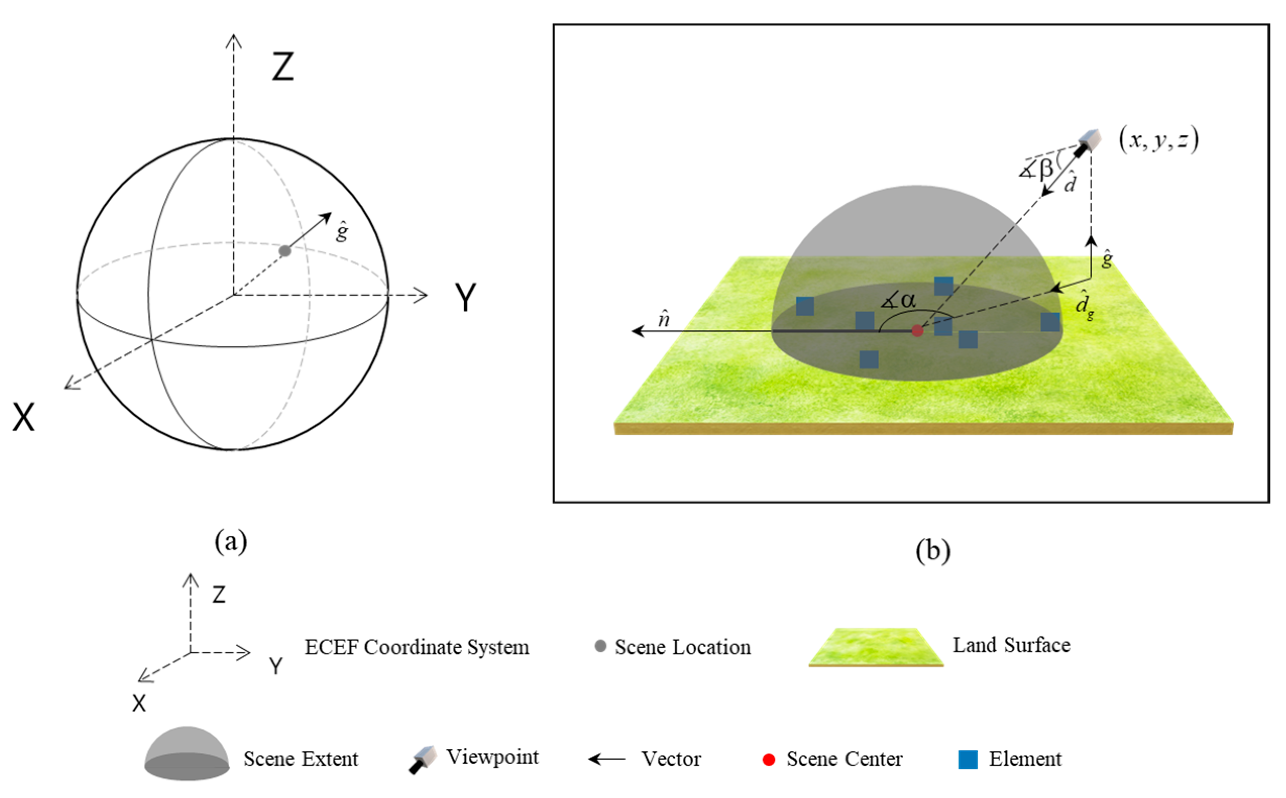
2.2. Spatial Reference and Viewpoint Orientation
- (1)
- The ground normal vector is calculated, and its unit vector is defined as :
- (2)
- The north vector is the projection of the vector onto the ground plane, with its unit vector defined as :
- (3)
- The viewpoint direction vector and the projection of this vector onto the ground are also calculated as , with the corresponding unit vectors defined as and :
- (4)
- The heading and pitch angles are computed by determining the clockwise angle relative to the north vector, which is derived by comparing the viewpoint’s longitude with the scene’s center point longitude , and the angle between the viewpoint direction vector and the ground normal vector, respectively:
2.3. Element Evaluation
2.4. Viewpoint Information Quantification
- (1)
- Calculation of the projected area when a polygon element, is defined by a set of vertices where is the index of each vertex, is considered:
- (2)
- When a polyline element, defined by a set of vertices with width is , the calculation method of its projected area is as follows:
- (3)
- When is a point element, the corresponding projected area is calculated according to its specific visualization method.
2.5. Viewpoint Search and Determination
3. Experiment
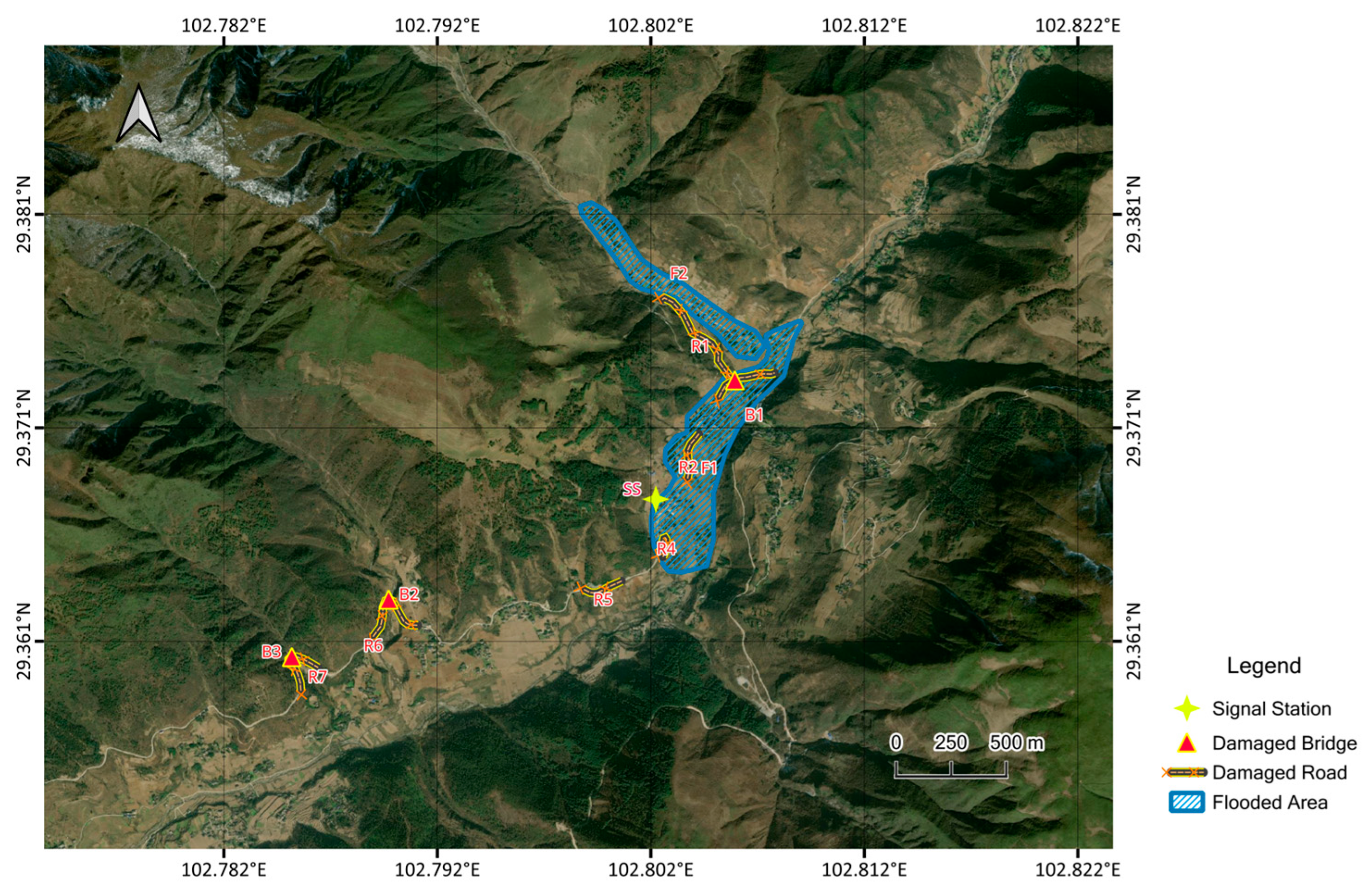
3.1. Data
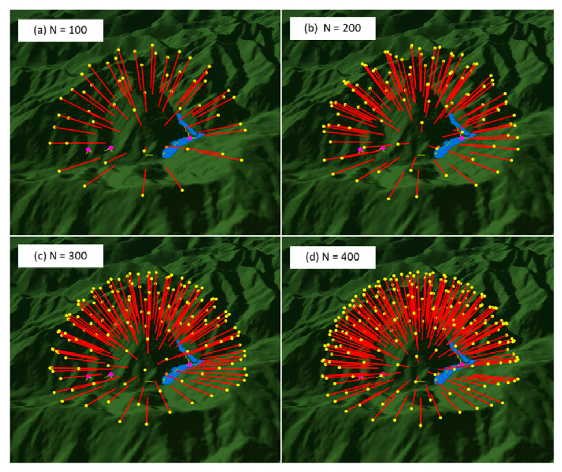
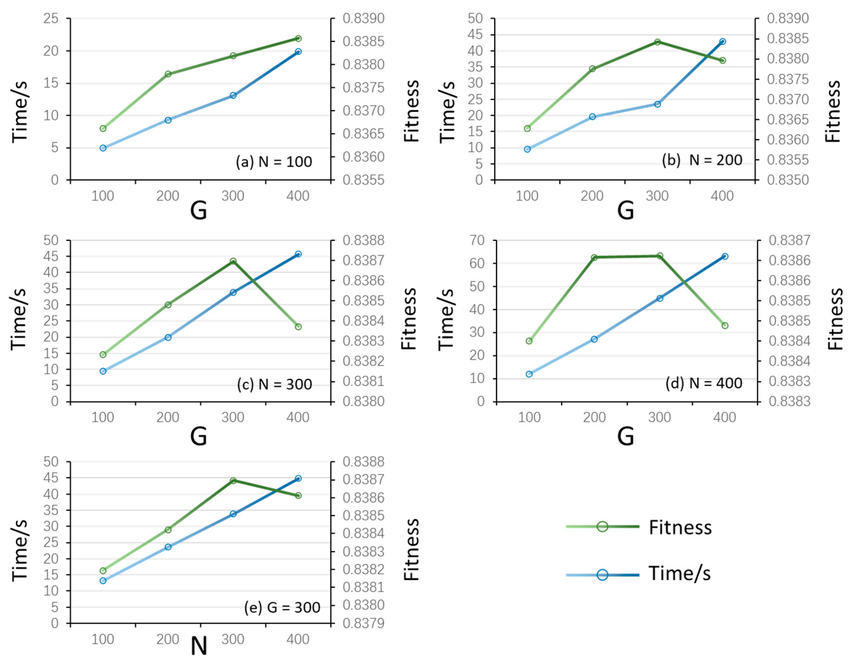
3.2. Parameters Analysis
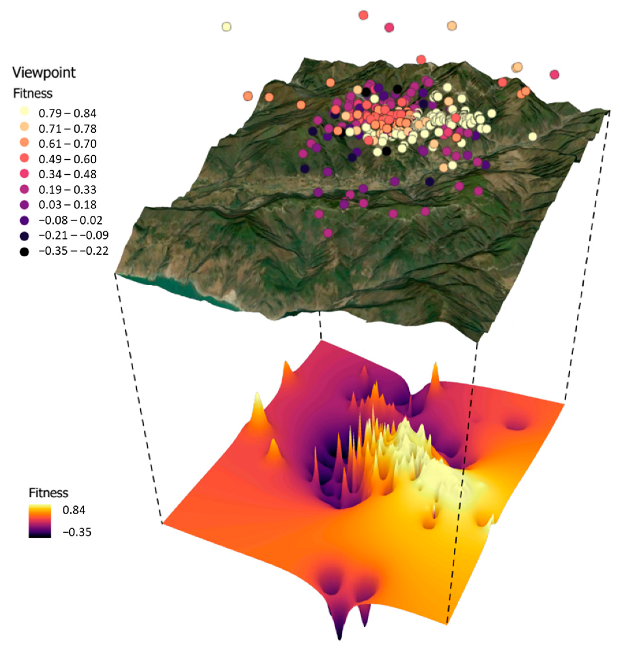
3.3. Result and Analysis
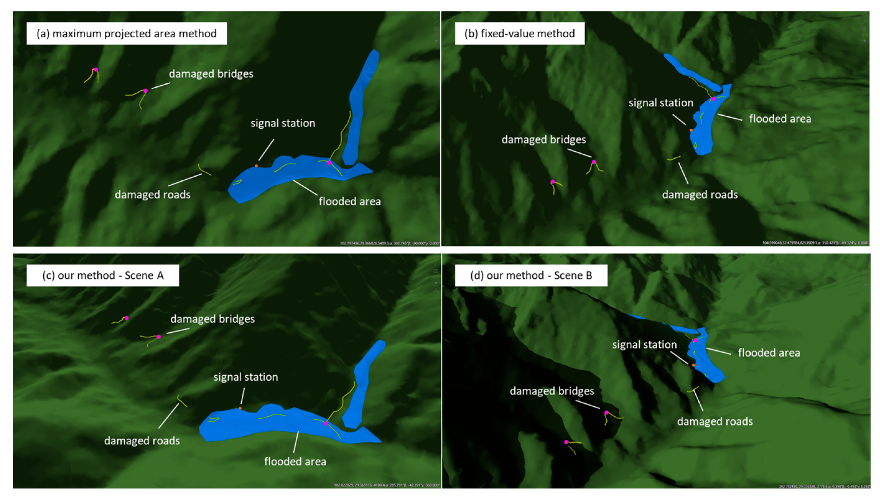
3.4. Discussion
4. Conclusions
5. Software
Author Contributions
Funding
Data Availability Statement
Conflicts of Interest
References
- Su, S.; Wang, L.; Du, Q.; Zhang, J.; Kang, M.; Weng, M. Revisiting Narrative Maps: Fundamental Theoretical Issues and a Research Agenda. Acta Geod. Cartogr. Sin. 2023, 52, 168–186. [Google Scholar] [CrossRef]
- Roth, R.E. Cartographic Design as Visual Storytelling: Synthesis and Review of Map-Based Narratives, Genres, and Tropes. Cartogr. J. 2021, 58, 83–114. [Google Scholar] [CrossRef]
- Wood, D. The Power of Maps; Guilford Press: New York, NY, USA, 1992; ISBN 978-0-89862-492-2. [Google Scholar]
- Bodenhamer, D.J.; Corrigan, J.; Harris, T.M. Deep Maps and Spatial Narratives; Indiana University Press: Bloomington, IN, USA, 2015; ISBN 978-0-253-01555-6. [Google Scholar]
- A’rachman, F.R.; Setiawan, C.; Hardi, O.S.; Insani, N.; Alicia, R.N.; Fitriani, D.; Hafizh, A.R.; Alhadin, M.; Mozzata, A.N. Designing Effective Educational Storymaps for Flood Disaster Mitigation in the Ciliwung River Basin: An Empirical Study. IOP Conf. Ser. Earth Environ. Sci. 2024, 1314, 012082. [Google Scholar] [CrossRef]
- Tasliya, R.; Fatimah, E.; Umar, M. Investigating the Impact of Story Maps in Developing Students’ Spatial Abilities on Hydrometeorological Disasters for E-Portfolio Assignments. Int. J. Soc. Sci. Educ. Econ. Agric. Res. Technol. 2023, 2, 459–475. [Google Scholar] [CrossRef]
- Carrard, P. Mapped Stories: Cartography, History, and the Representation of Time in Space. Front. Narrat. Stud. 2018, 4, 263–276. [Google Scholar] [CrossRef]
- Li, J.; Xia, H.; Qin, Y.; Fu, P.; Guo, X.; Li, R.; Zhao, X. Web GIS for Sustainable Education: Towards Natural Disaster Education for High School Students. Sustainability 2022, 14, 2694. [Google Scholar] [CrossRef]
- Lv, G.N.; Yu, Z.Y.; Yuan, L.W.; Luo, W.; Zhou, L.C.; Wu, M.G.; Sheng, Y.H. Is the Future of Cartography the Scenario Science? J. Geo-Inf. Sci. 2018, 20, 5–10. [Google Scholar]
- Dong, W.; Liao, H.; Zhan, Z.; Liu, B.; Wang, S.; Yang, T. New Research Progress of Eye Tracking-Based Map Cognition in Cartography since 2008. Acta Geogr. Sin. 2019, 74, 599–614. [Google Scholar]
- Liu, B.; Dong, W.; Wang, Y.; Zhang, N. The Influence of FOV and Viewing Angle on the VisualInformation Processing of 3D Maps. J. Geo-Inf. Sci. 2015, 17, 1490–1496. [Google Scholar]
- Blanz, V.; Tarr, M.J.; Bülthoff, H.H. What Object Attributes Determine Canonical Views? Perception 1999, 28, 575–599. [Google Scholar] [CrossRef]
- Stewart, E.E.M.; Fleming, R.W.; Schütz, A.C. A Simple Optical Flow Model Explains Why Certain Object Viewpoints Are Special. Proc. R. Soc. B 2024, 291, 20240577. [Google Scholar] [CrossRef]
- Shen, Y.; Yajie, X.; Yu, L. Elements and Organization of Narrative Maps: A Element-Structure-Scene Architecture Based on the Video Game Perspective. Acta Geod. Cartogr. Sin. 2024, 53, 967–980. [Google Scholar]
- Bing-Jie, L.; Chang-Bin, W. An Optimal Viewpoint Selection Approach for 3D Cadastral Property Units Considering Human Visual Perception. Geogr. Geo-Inf. Sci. 2023, 39, 3–9. [Google Scholar]
- Câmara, G.; Egenhofer, M.J.; Fonseca, F.; Vieira Monteiro, A.M. What’s in an Image? In Spatial Information Theory; Montello, D.R., Ed.; Lecture Notes in Computer Science; Springer: Berlin/Heidelberg, Germany, 2001; Volume 2205, pp. 474–488. ISBN 978-3-540-42613-4. [Google Scholar]
- Vázquez, P.-P.; Feixas, M.; Sbert, M.; Heidrich, W. Viewpoint Selection Using Viewpoint Entropy. In Proceedings of the Vision Modeling and Visualization Conference 2001; Aka GmbH: Frankfurt, Germany, 2001; pp. 273–280. [Google Scholar]
- Page, D.L.; Koschan, A.F.; Sukumar, S.R.; Roui-Abidi, B.; Abidi, M.A. Shape Analysis Algorithm Based on Information Theory. In Proceedings of the 2003 International Conference on Image Processing (Cat. No. 03CH37429), Barcelona, Spain, 14–17 September 2003; Volume 1, pp. I-229–I-232. [Google Scholar]
- Lee, C.H.; Varshney, A.; Jacobs, D.W. Mesh Saliency. ACM Trans. Graph. 2005, 24, 659–666. [Google Scholar] [CrossRef]
- Zhang, F.; Li, M.; Wang, X.; Wang, M.; Tang, Q. 3D Scene Viewpoint Selection Based on Chaos-Particle Swarm Optimization. In Proceedings of the Seventh International Symposium of Chinese CHI, Xiamen, China, 27 June 2019; ACM: New York, NY, USA, 2019; pp. 97–100. [Google Scholar]
- Häberling, C.; Bär, H.; Hurni, L. Proposed Cartographic Design Principles for 3D Maps: A Contribution to an Extended Cartographic Theory. Cartographica 2008, 43, 175–188. [Google Scholar] [CrossRef]
- Schmidt, M.; Delazari, L. Gestalt Aspects for Differentiating the Representation of Landmarks in Virtual Navigation. Cartogr. Geogr. Inf. Sci. 2013, 40, 159–164. [Google Scholar] [CrossRef]
- Liu, Z.; Ma, J.; Pan, X. Optimal Viewpoint Extraction Algorithm for Three-Dimensional Model Based on Features Adaption. J. Comput. Aided Des. Comput. Graph. 2014, 26, 1774–1780. [Google Scholar]
- Zhang, Y.; Fei, G.; Yang, G. 3D Viewpoint Estimation Based on Aesthetics. IEEE Access 2020, 8, 108602–108621. [Google Scholar] [CrossRef]
- Cao, W.; Hu, P.; Li, H.; Lin, Z. Canonical Viewpoint Selection Based on Distance-Histogram. J. Comput. Aided Des. Comput. Graph. 2010, 22, 1515–1521. [Google Scholar]
- Neuville, R.; Pouliot, J.; Poux, F.; Billen, R. 3D Viewpoint Management and Navigation in Urban Planning: Application to the Exploratory Phase. Remote Sens. 2019, 11, 236. [Google Scholar] [CrossRef]
- Panpan, J.; Yanyang, Z.; Yunxia, F. Best Viewpoint Selection for 3D Visualization Using Particle Swarm Optimization. J. Syst. Simul. 2017, 29, 156–162. [Google Scholar] [CrossRef]
- Poppe, M. QuickHull3D. Available online: https://github.com/mauriciopoppe/quickhull3d (accessed on 24 December 2024).


| Title | Description | |
|---|---|---|
| Scene A | Sudden Flash Flood | At about 2:30 a.m. on 20 July 2024, a flash flood occurred in Xinhua Village, Malie Township, Hanyuan County, Ya’an City, as a result of heavy rainfall, disrupting signals, roads, and bridges. |
| Scene B | Traffic Conditions Return | By 9:21 a.m. on 22 July 2024, both small bridges to the disaster area had been restored. Doufushi Bridge was reopened earlier that morning with a temporary emergency bridge, and a heavy-duty steel bridge was installed later to meet flood season and reconstruction needs. |
| Name | Id | Geometry Type |
|---|---|---|
| Flooded Area 1# | F1 | Polygon |
| Flooded Area 2# | F2 | Polygon |
| Damaged Road 1# | R1 | Polyline |
| Damaged Road 2# | R2 | Polyline |
| Damaged Road 3# | R3 | Polyline |
| Damaged Road 4# | R4 | Polyline |
| Damaged Road 5# | R5 | Polyline |
| Damaged Road 6# | R6 | Polyline |
| Damaged Road 7# | R7 | Polyline |
| Signal Station | SS | Point |
| Damaged Bridge 1# | B1 | Point |
| Damaged Bridge 2# | B2 | Point |
| Damaged Bridge 3# | B3 | Point |
| Element Id | NR | VS-Max | VS-Fixed | VS-CPSO |
|---|---|---|---|---|
| *F1 | 1.0000 | 8.3559 × 10⁻³ | 8.1118 × 10⁻³ | 1.3010 × 10⁻² |
| R2 | 0.8315 | 2.0557 × 10⁻⁴ | 1.0091 × 10⁻⁴ | 1.2151 × 10⁻⁴ |
| R3 | 0.6984 | 1.2787 × 10⁻⁴ | 2.4231 × 10⁻⁴ | 2.6994 × 10⁻⁴ |
| B1 | 0.6839 | 9.6880 × 10⁻⁵ | 9.6880 × 10⁻⁵ | 9.6880 × 10⁻⁵ |
| SS | 0.6177 | 4.3058 × 10⁻⁵ | 4.3058 × 10⁻⁵ | 4.3058 × 10⁻⁵ |
| R1 | 0.5616 | 5.2424 × 10⁻⁴ | 3.0681 × 10⁻⁴ | 3.7913 × 10⁻⁴ |
| R4 | 0.5484 | 1.7082 × 10⁻⁴ | 1.0009 × 10⁻⁴ | 1.1906 × 10⁻⁴ |
| F2 | 0.4637 | 2.7533 × 10⁻³ | 2.1064 × 10⁻³ | 3.2765 × 10⁻³ |
| R5 | 0.4593 | 8.7834 × 10⁻⁵ | 2.0996 × 10⁻⁴ | 2.4224 × 10⁻⁴ |
| B2 | 0.3408 | 9.6880 × 10⁻⁵ | 9.6880 × 10⁻⁵ | 9.6880 × 10⁻⁵ |
| R6 | 0.3362 | 4.2096 × 10⁻⁴ | 3.4138 × 10⁻⁴ | 4.2183 × 10⁻⁴ |
| B3 | 0.2956 | 9.6880 × 10⁻⁵ | 9.6880 × 10⁻⁵ | 9.6880 × 10⁻⁵ |
| R7 | 0.2946 | 3.7097 × 10⁻⁴ | 2.7704 × 10⁻⁴ | 3.5369 × 10⁻⁴ |
| Element Id | NR | VS-Max | VS-Fixed | VS-CPSO |
|---|---|---|---|---|
| *B2 | 1 | 9.69 × 10⁻⁵ | 9.69 × 10⁻⁵ | 2.06 × 10⁻⁴ |
| *B3 | 1 | 9.69 × 10⁻⁵ | 9.69 × 10⁻⁵ | 2.06 × 10⁻⁴ |
| R7 | 0.7487 | 3.71 × 10⁻⁴ | 2.77 × 10⁻⁴ | 3.48 × 10⁻⁴ |
| R6 | 0.7324 | 4.21 × 10⁻⁴ | 3.41 × 10⁻⁴ | 4.17 × 10⁻⁴ |
| R5 | 0.3800 | 8.78 × 10⁻⁵ | 2.10 × 10⁻⁴ | 1.70 × 10⁻⁴ |
| R4 | 0.3555 | 1.71 × 10⁻⁴ | 1.00 × 10⁻⁴ | 1.53 × 10⁻⁴ |
| SS | 0.3515 | 4.31 × 10⁻⁵ | 4.31 × 10⁻⁵ | 9.16 × 10⁻⁵ |
| F1 | 0.3265 | 8.36 × 10⁻³ | 8.11 × 10⁻³ | 7.44 × 10⁻³ |
| B1 | 0.3177 | 9.69 × 10⁻⁵ | 9.69 × 10⁻⁵ | 2.06 × 10⁻⁴ |
| R1 | 0.3175 | 5.24 × 10⁻⁴ | 3.07 × 10⁻⁴ | 3.56 × 10⁻⁴ |
| R3 | 0.3163 | 1.28 × 10⁻⁴ | 2.42 × 10⁻⁴ | 1.99 × 10⁻⁴ |
| F2 | 0.3109 | 2.75 × 10⁻³ | 2.11 × 10⁻³ | 1.80 × 10⁻³ |
| R2 | 0.2160 | 2.06 × 10⁻⁴ | 1.01 × 10⁻⁴ | 1.63 × 10⁻⁴ |
| Method | Fitness | Vote |
|---|---|---|
| Maximum projected area method | 0.37 | 4 |
| Fixed-value method | 0.38 | 5 |
| Our method | 0.84 | 17 |
Disclaimer/Publisher’s Note: The statements, opinions and data contained in all publications are solely those of the individual author(s) and contributor(s) and not of MDPI and/or the editor(s). MDPI and/or the editor(s) disclaim responsibility for any injury to people or property resulting from any ideas, methods, instructions or products referred to in the content. |
© 2025 by the authors. Published by MDPI on behalf of the International Society for Photogrammetry and Remote Sensing. Licensee MDPI, Basel, Switzerland. This article is an open access article distributed under the terms and conditions of the Creative Commons Attribution (CC BY) license (https://creativecommons.org/licenses/by/4.0/).
Share and Cite
Liu, S.; Wang, Y.; Tang, Q.; Han, Y. Viewpoint Selection for 3D Scenes in Map Narratives. ISPRS Int. J. Geo-Inf. 2025, 14, 219. https://doi.org/10.3390/ijgi14060219
Liu S, Wang Y, Tang Q, Han Y. Viewpoint Selection for 3D Scenes in Map Narratives. ISPRS International Journal of Geo-Information. 2025; 14(6):219. https://doi.org/10.3390/ijgi14060219
Chicago/Turabian StyleLiu, Shichuan, Yong Wang, Qing Tang, and Yaoyao Han. 2025. "Viewpoint Selection for 3D Scenes in Map Narratives" ISPRS International Journal of Geo-Information 14, no. 6: 219. https://doi.org/10.3390/ijgi14060219
APA StyleLiu, S., Wang, Y., Tang, Q., & Han, Y. (2025). Viewpoint Selection for 3D Scenes in Map Narratives. ISPRS International Journal of Geo-Information, 14(6), 219. https://doi.org/10.3390/ijgi14060219