PixelQuery: Efficient Distance Range Join Query Technique for Visualization Analysis

Abstract

A distance range join query (DRJQ) is a fundamental and critical operation in spatial database queries. It identifies geographic elements within specified distance ranges. This technique has a wide range of applications in multiple domains, including Geographic Information Systems (GISs), urban planning, and environmental monitoring. However, performing a DRJQ on large-scale spatial data remains a challenging problem, as the computational complexity of existing techniques escalates rapidly with increasing volumes of data. We propose PixelQuery, an efficient DRJQ method specifically optimized for visualization analysis. PixelQuery integrates spatial indexing with visualization-oriented strategies. It directly computes the display values of query results within the viewport, substantially lowering computational costs. Experiments conducted on datasets of varying scales demonstrate that this method can handle visualization queries involving tens of millions of elements on a standard laptop, with a maximum processing time of only 7.64 s. This technology provides a robust solution for rapid DRJQ processing and the visualization of large-scale vector data, offering promising potential for a diverse range of applications.

1. Introduction

In recent years, the volume of spatial data generated from diverse sources, such as smartphones and satellites, has grown exponentially across the world. For instance, as of 2023, the number of geographic vector point features in OpenStreetMap (OSM) has approached the billions, while the number of line vector features is nearing the same magnitude [1]. Distance join queries (DJQs) have attracted significant attention in the database community due to their critical role in applications spanning spatial databases [2], data mining [3], and multimedia databases [4]. The most representative queries include the k Nearest-Neighbor Join Query (kNNJQ), k Closest Pair Query (kCPQ), DRJQ, and distance join query (DJQ) [5]. This paper focuses on the DRJQ task, where a DRJQ finds, for each point in the set P, all points in the set Q that fall within a circular region with a radius of R centered at that point in P.

DRJQ has gained considerable attention due to its significance in real-world applications. Two representative application cases are presented in this paper: Application Case 1 (Agricultural Resource Management) involves an authority planning for the sustainable use of water resources while considering two key spatial datasets—the locations of rivers and the distribution of agricultural and pastoral areas. By utilizing a DRJQ, it is possible to “identify all river branches within a 5-kilometer radius of agricultural and pastoral regions”. This approach helps to pinpoint which river branches fall within the influence of these agricultural activities, thereby providing a scientific basis for water resource management and conservation (the borders or centroids of each land area can be used for this query). Application Case 2 (Emergency Health Control) involves health departments and considers two datasets—sources of disease outbreaks and potentially affected public places. A DRJQ can find all public places within 5 km of the sources of a disease to allow authorities to implement timely control measures.

The aforementioned application scenarios often require massive datasets for input and querying. A common approach to handling such large-scale data is through parallel and distributed processing. Consequently, several parallel algorithms for DJQs have been developed and executed within the framework of MapReduce [6] and Spark [7]. Recently, parallel algorithms for DRJQs [5] have been developed and implemented within frameworks such as SpatialHadoop [6] and LocationSpark [8]. These algorithms effectively partition tasks across distributed computing resources, enhancing query efficiency and response times, thus maintaining high performance even when processing voluminous spatial data. However, when Spark handles a DRJQ task, an increase in data volume puts enormous memory pressure on the device. In contrast, for SpatialHadoop, the growth of the volume of data exchanged during the map and reduce phases affects the query’s performance [5].

Machine learning methods have also been applied to address the challenges of DRJQs. In [9], a machine learning-based framework is proposed to tackle the complexity of spatial join operations in large-scale datasets. By establishing a cost model, this framework extracts key features from input datasets, such as data distribution and spatial partitioning, while considering the complexity of DRJQs to optimize computational performance. Although the proposed model demonstrates promising performance on large-scale real-world data, the model requires a substantial amount of training data and computational resources, resulting in high training costs. Additionally, it requires the selection and fine-tuning of multiple parameters. When dealing with different datasets, if the data distribution changes, it may require retraining and retuning, further increasing the cost of its utilization.

Indexing and optimizing indexes for datasets is also a primary direction for research into DJQs. In [10], a method was proposed that optimizes DRJQs using k2-tree indexing along with the setting of query windows. This approach reduces the query time by up to 30 times that of planar scan algorithms. However, the performance of this method is influenced by the position of the query window, which can significantly impact the performance of the query under certain special data distributions.

In addition, in many practical applications, visualization is an important step in data analysis. Visualizing the results of the query after completing a DRJQ helps users better understand the spatial relationships between different data elements and the distribution of elements that meet specific criteria. This visualization result can guide more targeted and fine-grained processing during subsequent data handling, thereby reducing unnecessary computational resource consumption. Within the complete query visualization workflow, visualization operations also face the challenge of performance degradation in big data scenarios. This makes it difficult for the entire process to meet real-time performance requirements and limits its effectiveness in specific practical application scenarios.

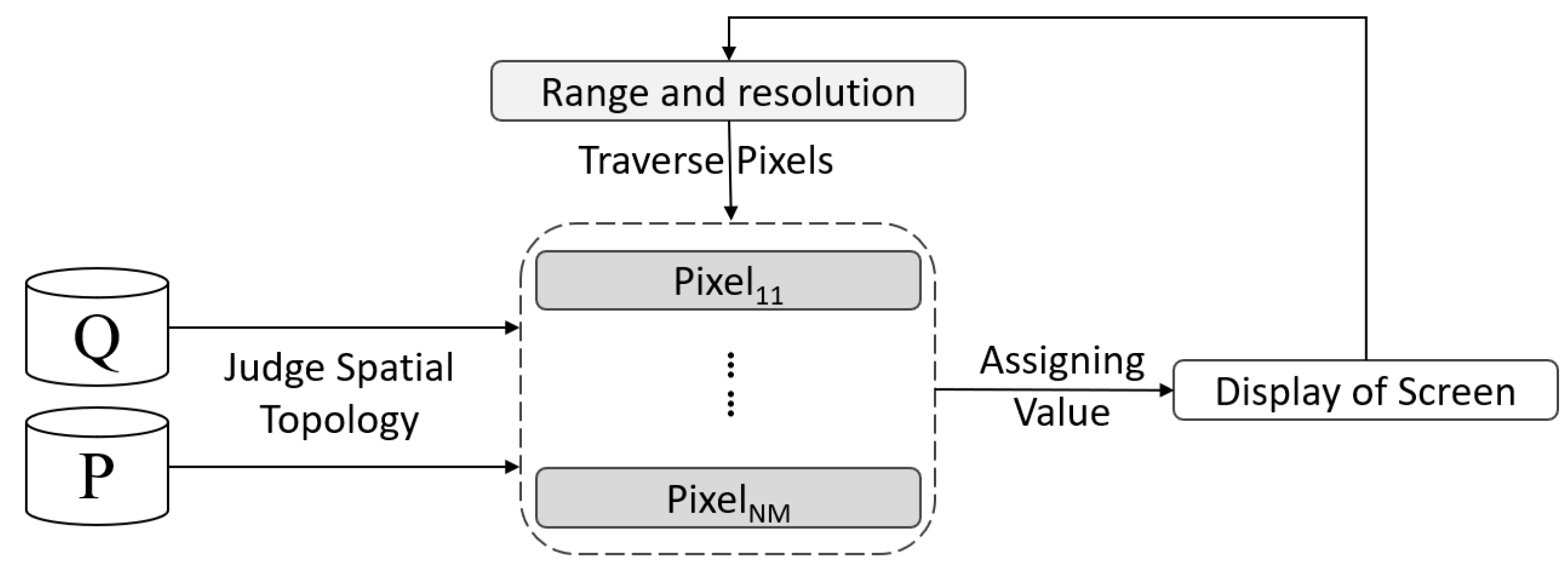
To address the aforementioned issues, we propose a display-driven vector data query visualization technique. Its processing flow is depicted in Figure 1. PixelQuery directly calculates the final pixel values for visualization. Its working principle can be concisely described as follows: The visualization is created by the pixel display values on the screen, where each pixel corresponds to a specific real-world geographic area. Determining pixel values only requires the presence of one object within the pixel that meets the query conditions, whereas data-driven methods require the judgment of all query objects within the pixel. By introducing an effective strategy based on spatial indexing, the calculation of pixel values based on spatial relationships becomes much faster. This approach significantly reduces redundant calculations between vectors during the query visualization process.

PixelQuery significantly enhances the efficiency of DRJQs through a pixel-level computation model, making it particularly suitable for the real-time visualization analysis of large-scale data across various scenarios.

The remainder of this paper is organized as follows: Section 3 describes the visualization-oriented distance range join query model (VODRJQ) and introduces the algorithm in detail. In Section 4, the advancement of the algorithm is verified through several groups of comparative experiments. Section 5 critically examines the algorithm’s limitations and proposes future directions for optimization. The conclusion is presented in Section 6.

2. Related Work

The topic of DJQs has attracted significant interest from the spatial database research community. Researchers have made contributions to their optimization that come from directions such as optimizing data partitioning strategies and query methods on Distributed Spatial Data Management Systems (DSDMSs), indexing input datasets, and improving and optimizing these indexes.

2.1. Spatial Data Distance Join Query

The kNNJQ MapReduce algorithm has been extensively studied in the academic literature. In [11], a kNNJQ MapReduce algorithm specifically designed for two-dimensional spatial data was introduced. This algorithm subdivides the data space into uniform cells and amalgamates adjacent cells if they contain fewer than k points, thereby guaranteeing the completeness of k-nearest neighbor (kNN) lists. An enhancement to this methodology replaces the merging process with a radius-based search around the query point, thus minimizing the number of distance calculations required. Voronoi diagram partitioning techniques [12,13] have been implemented to further improve kNNJQ algorithms, resulting in optimized data shuffling and reduced computational costs. One such technique [14] employs Voronoi diagrams to facilitate range and kNN search queries in two dimensions, effectively clustering data objects to enhance the efficiency of kNN candidate checking. However, this partitioning strategy may lead to data skew in large-scale datasets. In [15], an innovative exact and approximate MapReduce algorithm for parallel kNNJQs utilizing R-tree and Z-value-based partitioning methodologies was presented. The kCPQ and DJQ MapReduce algorithms incorporated within SpatialHadoop deploy plane-sweep techniques to efficiently determine the k-th closest pair. Furthermore, Mavrommatis et al. developed the SliceNBound algorithm in Apache Spark, which uses an efficient partitioning framework for closest pairs and distance join queries by systematically slicing the plane into strips. Nevertheless, the SliceNBound algorithm may lead to an unbalanced data distributions when dealing with large-scale data. The computing nodes responsible for processing a large amount of data can become a bottleneck, and their parallel processing capabilities cannot, therefore, be fully utilized. Recent advances [5] in the DRJQ algorithm have been made and successfully implemented within the SpatialHadoop and LocationSpark frameworks. These innovations involved the use of advanced repartitioning techniques, specifically the Grid and Quadtree methods, which have significantly improved execution times when processing large datasets using SpatialHadoop.

Numerous research efforts have focused on optimizing data structures, and specifically on enhancing spatial indexing mechanisms such as R-trees [16], quad-trees [17], and $xB{R}^{+}$-trees [18]. R-trees [19] are particularly essential for indexing datasets, especially when querying complex relationships known as distance join queries (DJQs). To improve the efficiency of these queries, several techniques have been proposed, including synchronized tree traversal, which can employ traversal orders like depth-first (DF) or best-first (BF) orders for the effective navigation of spatial indices [16]. A comprehensive experimental study [17] presents a comparative analysis of R*-trees versus quad-tree-like index structures within the context of DJQs, alongside their respective index construction methodologies. Their findings demonstrated that R*-trees perform exceptionally well when handling static datasets, underscoring their utility in scenarios involving relatively stable data.

Furthermore, research [18] has concentrated on developing specialized algorithms based on the $xB{R}^{+}$-tree architecture to tackle DJQs with greater efficiency. The $xB{R}^{+}$-tree is defined as a hierarchical pointer-based index structure optimized for disk storage, which is achieved through systematic spatial decomposition that facilitates the effective indexing of multidimensional points. In particular, experimental evaluations showed that the $xB{R}^{+}$-tree outperforms the R*-tree in handling DJQs, highlighting its advantages in managing complex spatial query effectively. In [10], a compact data structure, referred to as the k2-tree, which was designed for the efficient management of DJQs with a specific emphasis on the KCPQ and the εDJQ, was introduced. The algorithms proposed leverage the indexing capabilities inherent in the k2-tree and enhance tree traversals through the utilization of bitmaps and optimized operations on these bitmaps. Consequently, the performance of these algorithms surpasses that of conventional plane-sweep methods, demonstrating enhancements in both speed and memory utilization.

2.2. Display-Driven Visualization Computing

When dealing with large-scale geographic vector data, different computing frameworks each have their own unique advantages but inevitably also have some limitations.

SpatialHadoop [20] optimizes the processing of geographic vector data by providing spatial partitioning algorithms (such as space-filling curve partitioning and grid partitioning). However, the complexity of these algorithms is relatively high. In large-scale datasets especially, the computational overhead increases significantly with the growth in the volume of data used. The partition of the space-filling curve requires sorting and mapping all data, which consume a large amount of computational resources. In addition, when performing spatial queries, SpatialHadoop needs to scan and calculate a large amount of data, resulting in a prolonged response time to the query. Similar problems also occur in Apache Sedona [21]. When dealing with large-scale geographic vector data, it faces challenges in data partitioning and node load balancing and has high CPU and memory resource requirements. Its partitioning strategy may not be able to dynamically adapt to changes in data distribution, leading to a decrease in processing efficiency.

Display-driven computing (DisDC) is a computing model that is especially suitable for data-intensive problems in GISs. In DisDC, the computing units are pixels rather than spatial objects. This simplifies the problems of data partitioning and computational load, enabling high-performance parallel computing. The core aim in DisDC is to identify the spatial relationships between pixels and spatial objects, thus determining the value of the pixels in the display. DisDC has broad potential for applications and research into big data analysis. In our previous work [22,23,24,25], the primary idea behind DisDC was first proposed and then applied to solve some basic analysis problems in GISs. We have successively brought forward HiBuffer and HiBO to provide interactive buffers and overlay analyses of large-scale spatial data. In this paper, we apply DisDC to DRJQs and the visualization of large-scale spatial vector data, exploring its effectiveness.

3. Methodology

In this section, the key technologies involved in PixelQuery are introduced. For simplicity, we refer to the queried vector dataset as the target dataset ($T_d$) and its vector objects as target vectors ($t_{v}s$). Correspondingly, the vector dataset used as the query condition (in a DRJQ, this consists of the sum of circular regions with a radius equal to the distance threshold, centered on each of the features of the dataset) is referred to as the reference dataset ($R_d$), and its objects are called reference vectors ($r_{v}s$).

To introduce the semantic details of the DRJQ studied in this paper, we define the DRJQ while assuming that the Euclidean distance, dist, is the distance used throughout this article. The DRJQ, given two point datasets (${\mathbb{T}}_d$ and ${\mathbb{R}}_d$) and a distance threshold $R_B$, finds, for each point $r_{vi}\in {\mathbb{R}}_d$, all the points in ${\mathbb{T}}_d$ that fall within the circular shape centered on $r_{vi}$ with radius $R_B$. Its formal definition is as follows below.

Theorem 1.

Definition of the DRJQ.

Let ${\mathbb{R}}_d=\{r_{v0},r_{v1},\dots ,r_{vn-1}\}$ and ${\mathbb{T}}_d=\{t_{v0},t_{v1},\dots ,t_{vm-1}\}$ be two sets of points in $E^d$, and the distance threshold $R_B\in {\mathbb{R}}^{+}$. Then, the result of the DRJQ is a set DRJ$({\mathbb{R}}_d,{\mathbb{T}}_d,$ $R_B)\subseteq {\mathbb{R}}_d\times {\mathbb{T}}_d$, which contains for each point of ${\mathbb{R}}_d(r_{vi}\in {\mathbb{R}}_d)$ all points from ${\mathbb{T}}_d(t_{vi}\in {\mathbb{T}}_d)$ that fall in the circular shape centered on $r_{vi}$ with radius $R_B$:

$$\mathrm{DRJ}({\mathbb{R}}_d,{\mathbb{T}}_d,R_B)=\{(r_{vi},t_{vj}):r_{vi}\in {\mathbb{R}}_d,t_{vj}\in {\mathbb{T}}_d,dist(r_{vi},t_{vj})\le R_B\}$$

(1)

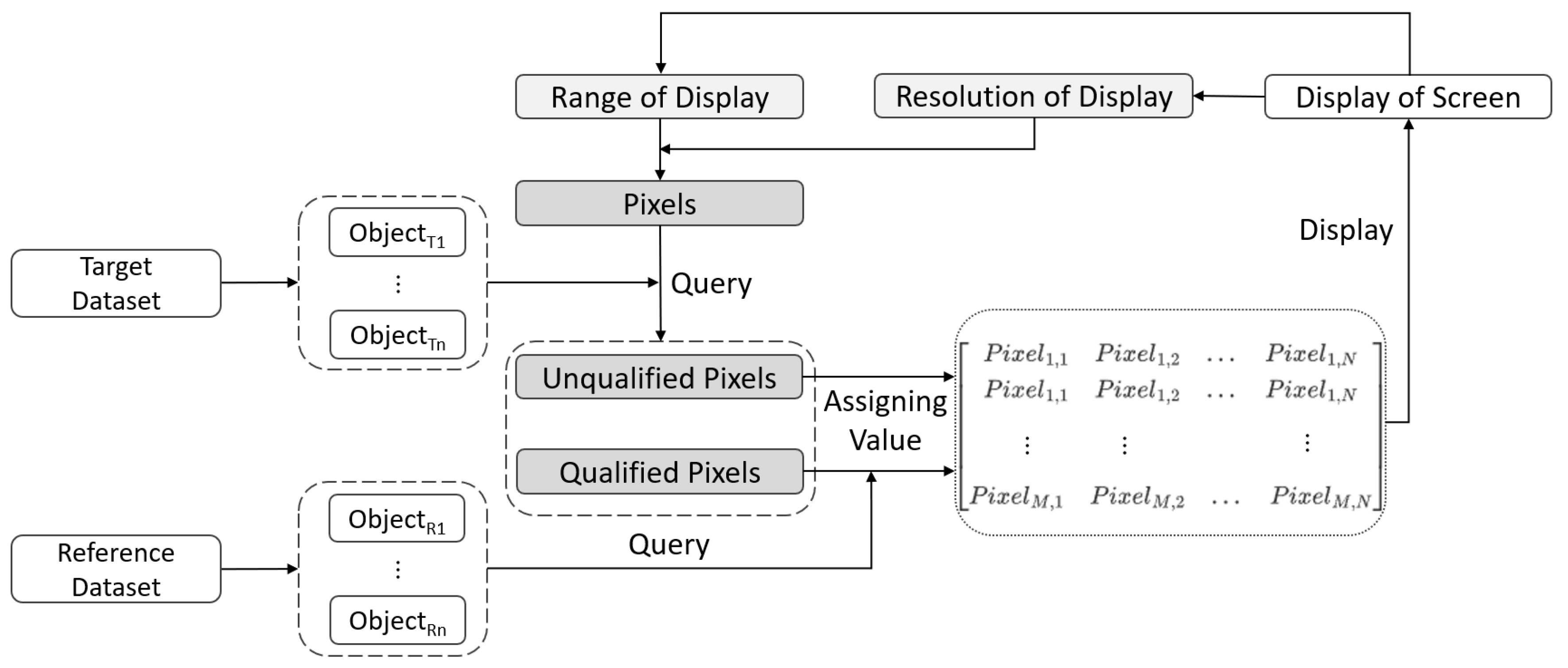
Specifically, we propose a model called the visualization-oriented DRJQ (VODRJQ), which is illustrated in Figure 2. This model takes screen pixels as its computation units. It traverses the pixels to check if there are vector objects within the current pixel range. Then, it determines whether these objects have spatial relationships with other vector objects. Based on these steps, the visualization result of the pixels is determined. According to the visualization-oriented spatial join query model and Equation (1), the spatial join query problem can be transformed into the evaluation of two spatial relationships between the position of pixels and vector objects:

• The spatial relationship between the geographic location of the pixel and the $t_{v}s$, i.e., whether the vector objects of the $T_d$ are within the spatial range represented by the pixel point.
• The spatial relationship between $r_{v}s$ and $t_{v}s$, i.e., whether the $t_{v}s$ within the pixel point meet the preset spatial query conditions when considering vector objects from another dataset.

3.1. Data Organization and Algorithm Overview

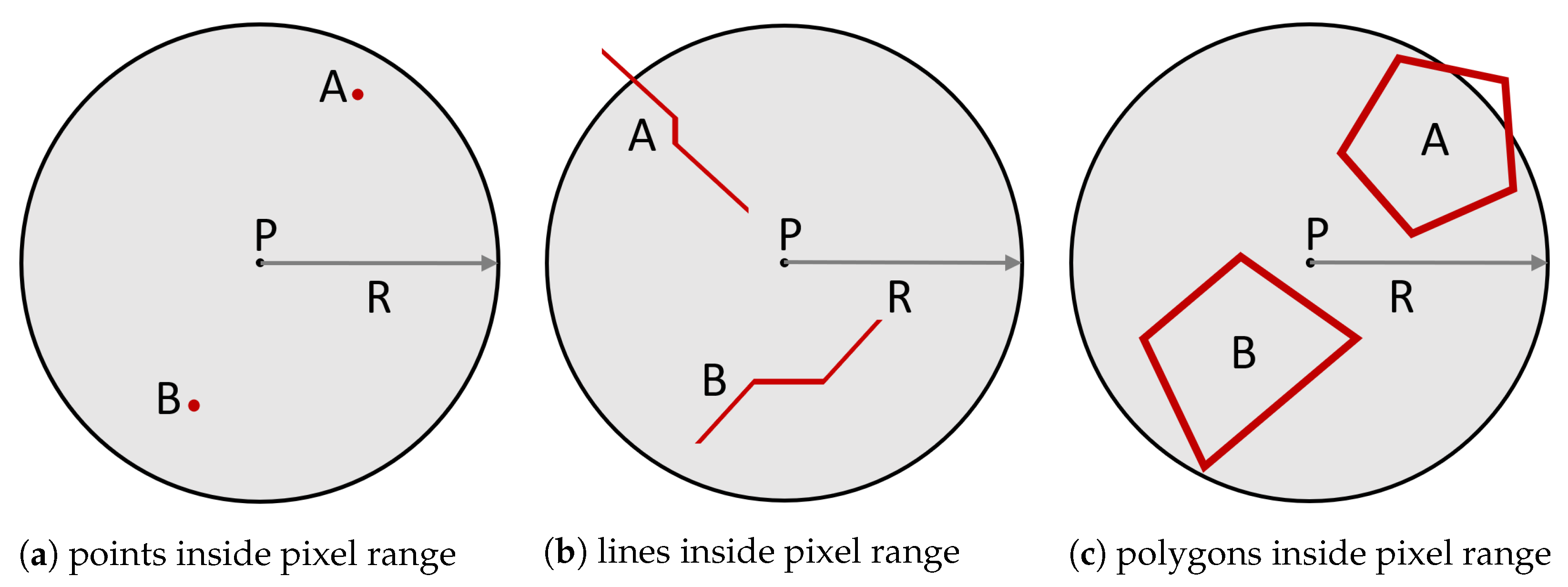
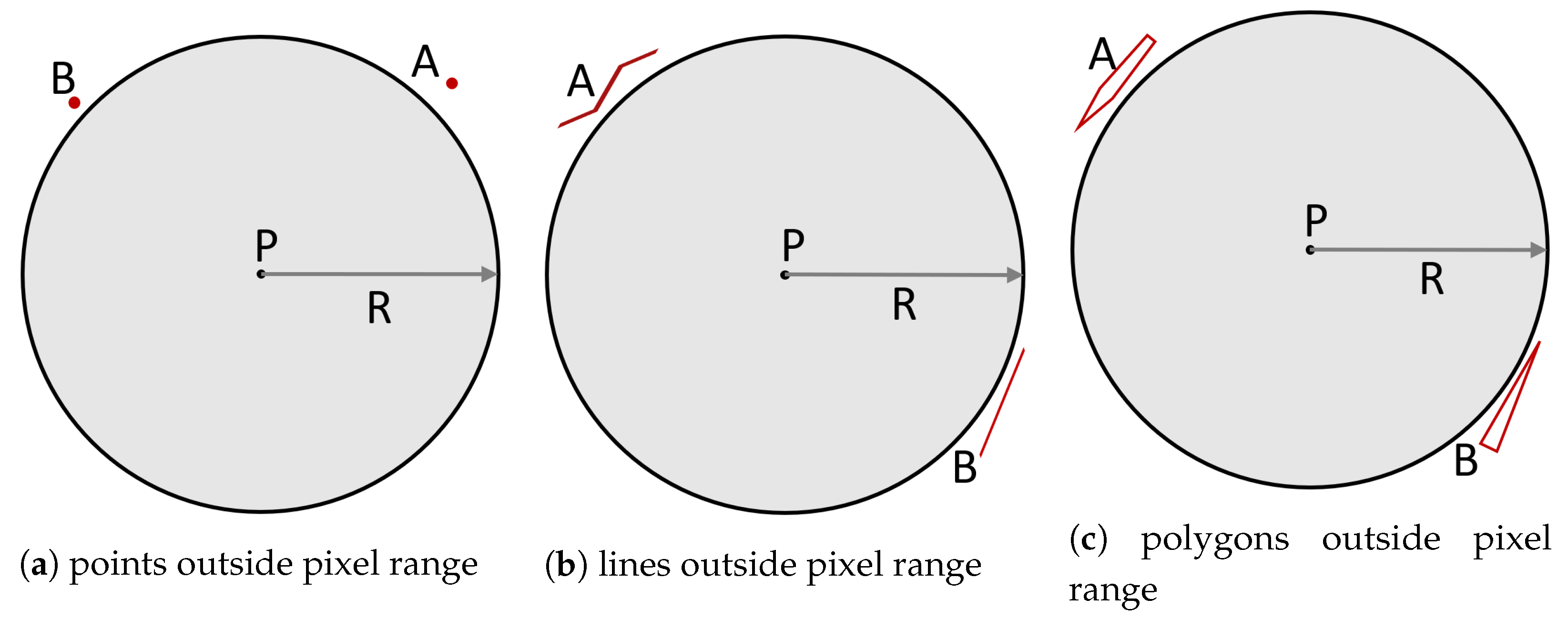
To address spatial relationship problem 1, we need to determine whether the $t_{v}s$ are within the radius R of pixel P. As shown in Figure 3 and  Figure 4, for point objects, the condition is that they are located within the pixel’s range; for line objects, the condition is that the line feature is entirely within the pixel’s range or partially within the pixel; similarly, for polygon objects, the condition is that the polygon is entirely within the pixel’s range or that the spatial extent of the polygon overlaps with the spatial extent of the pixel. This can be abstracted to checking whether a circle centered at P with radius R intersects with any elements of the $t_v$. An intuitive solution to this problem is as follows: use the INTERSECT operator provided by the R-tree within the range of a circle centered at pixel P with radius R to determine if the circle intersects with any $t_v$ objects.

Accordingly, to address spatial problem 2, we extend the definitions in Theorem 1. Figure 5 illustrates the DRJ query regions for different types of objects when the distance threshold is $R_B$. For line vectors, the distance threshold $R_B$ should be extended to the union of circular regions with radius $R_B$ centered at each point on the line vector, which is the spatial buffer zone of the line vector with radius $R_B$. For polygons, the distance threshold should be extended to the union of the spatial buffer zone of the boundary and include the space within the polygon.

However, in actual query operations, using Minimum Bounding Rectangles (MBRs) for queries is more efficient than using a circle, and the R-tree is especially suitable for bounding box queries. Therefore, we used the R-tree to organize the data at a fine-grained level. For point and line objects, we created an R-tree index with points and segments as node types; for polygon objects involving the filling step, we used a Multi-Level Index Architecture (MLIA) [24]. In  the MLIA, each edge of a polygon object is stored as a segment, and the MBRs of polygons are stored as boxes. Specifically, to support spatial judgment in the VOSJQ, two operations are performed: (1) the identification of node information (parallel to), including whether an edge is parallel to the x-axis; (2) a segmented cutting process for monotonically increasing or decreasing edges. The overall data structure is shown in

Table 1. Vector data organization in PixelQuery.

Data Type	Data Element	Data Management
Point	Discrete point	RtreeP{point(x,y),ID}
Linestring	Separate or connected segments	RtreeL{segment$(poin{t}_i,poin{t}_{i+1})$, ID}
Polygon	Multiple end-to-end segments	RtreeE{$segment(poin{t}_i,poin{t}_{i+1}),IP,ID$} RtreeMBR{$box(point(x_{min},y_{min}),point(x_{max},y_{max}))$}

.

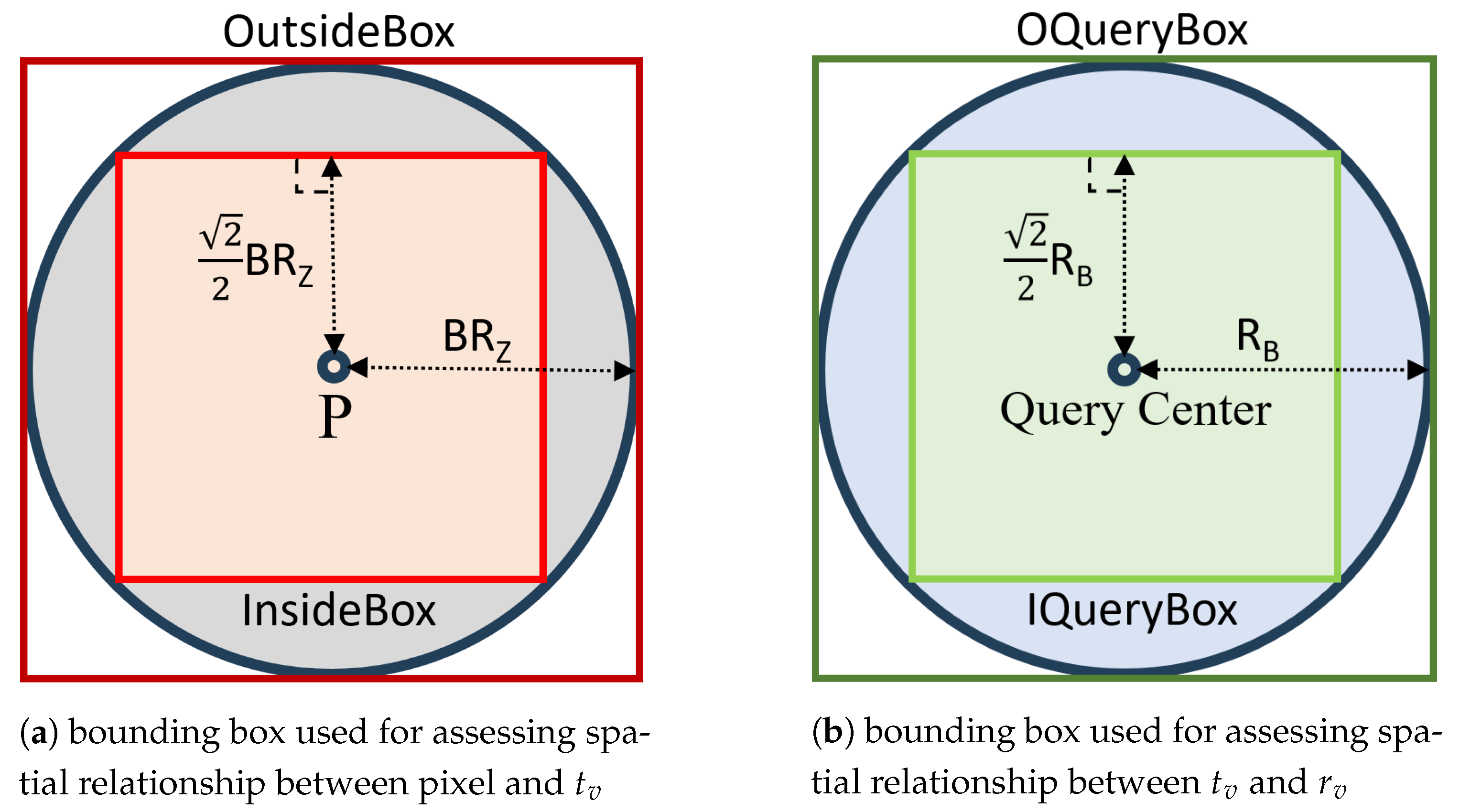
Meanwhile, we constructed multiple auxiliary query boxes to accelerate the query process, as shown in Figure 6. The InsideBox and OutsideBox are used to determine whether there are $t_v$s within the pixel, simplifying the circle query into a joint query of two bounding boxes. Similarly, the OQueryBox and IQueryBox are used to judge the distance relationships between $t_v$s and $r_v$s.

B is the pixel radius of the final visualization object, and $R_z$ is its resolution at the Z-th level. InsideBox has a side length of $2R_1$ and OutsideBox has a side length of $2R_2$. IQueryBox has a side length of $2R_{B1}$ and OQueryBox has a side length of $2R_{B2}$.

3.2. Distance Range Join Query Algorithm

Based on our analysis, we have proposed two corresponding algorithms to handle the DRJQ of different spatial objects: the linestring-point objects distance range join query (LPDRJQ) algorithm (Algorithm 1) and polygon-objects-involving distance join range query (PIDRJQ) algorithm. The LPDRJQ algorithm is designed to handle spatial connectivity query issues between point and line objects, while the PIDRJQ algorithm is intended for spatial connectivity queries when at least one of the $t_{v}s$ or $r_{v}s$ is of a polygon data type, as it requires consideration of the polygon’s boundaries and extent.

Figure 7 illustrates the processing flow of the visualization-oriented algorithm. First, determine whether the categories of the query object and the queried object contain polygons, and then use the MLIA to construct an R-tree spatial index. At the same time, check the display range of the screen, determine the size of the display domain and the zoom level to obtain the range of the mapping and the central position coordinates of each pixel in the actual geographical space. If there are polygon features in the query, use PIDRJQ; if not, use LPDRJQ. Traverse each pixel in the display domain and determine whether the spatial distance relationships between $t_v$s and pixels, and between $t_v$s and $r_v$s, meet the query conditions. Then, assign values to the display values of the pixels and update the visualization results on the screen. If the range or resolution of the display domain changes, update the corresponding attributes of the pixels and perform the query again.

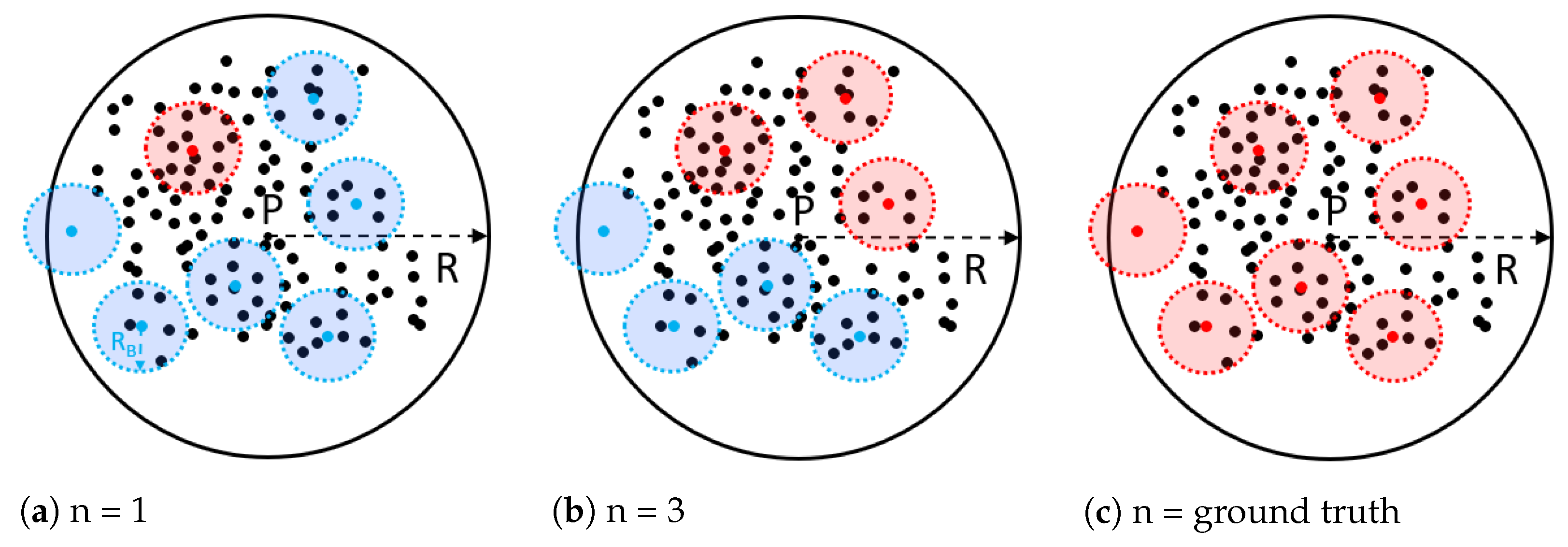
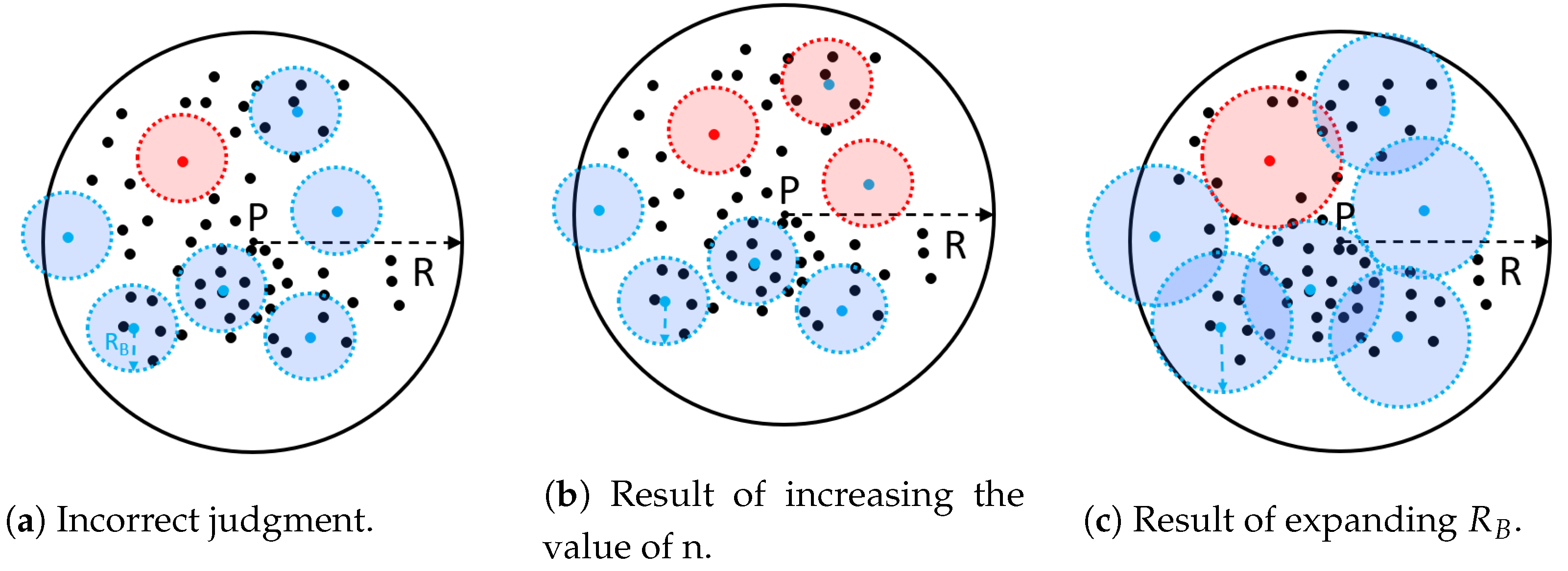
We have introduced an adjustable parameter n into the algorithm, which represents the sampling of n $t_v$s within a pixel as query objects. Its value affects the accuracy and speed of the query. In Section 4.1, we discuss the impact of n on the algorithm’s performance under different circumstances. Figure 8 illustrates the spatial relationships within a pixel using two point datasets, thus demonstrating the situations where n is set to 1, 3, and the ground truth. In this figure, the blue points represent $t_v$s that have not been queried, the black points represent $r_v$s, and the red points represent the $t_v$s serving as query centers in the LPDRJQ algorithm. In data-dense querying scenarios, querying just a small number of $t_v$s can yield the displayed results for the pixel. The spatial Euclidean distance is defined as dist.

Algorithm 1 LPDRJQ

Require:  Pixel P, pixel radius B, resolution $R_z$, distance threshold $R_B$, $R_d$ spatial index $\mathbf{R}tre{e}_{\mathbf{ref}}(\mathbf{R}tree\mathbf{P},\mathbf{R}tree\mathbf{L})$, $T_d$ spatial index $\mathbf{R}tre{e}_{\mathbf{tar}}(\mathbf{R}tree\mathbf{P},\mathbf{R}tree\mathbf{L})$, query factor n Ensure:  True, False (False: P without $t_{v}s$ satisfying DRJQ with distance threshold $R_B$; True: P within $t_{v}s$ satisfying DRJQ with distance threshold $R_B$) 1: $R_1\leftarrow {\displaystyle \frac{\sqrt{2}}{2}}B\times R_z$; $R_2\leftarrow B\times R_z$; $R_{B1}\leftarrow {\displaystyle \frac{\sqrt{2}}{2}}\times R_B$; $R_{B2}\leftarrow R_B$ 2: $\mathit{InsideBox}\leftarrow BOX({\mathbf{P}}_{.y-R_1},{\mathbf{P}}_{.x-R_1},{\mathbf{P}}_{.y+R_1},{\mathbf{P}}_{.x+R_1})$ 3: $\mathit{OutsideBox}\leftarrow BOX({\mathbf{P}}_{.y-R_2},{\mathbf{P}}_{.x-R_2},{\mathbf{P}}_{.y+R_2},{\mathbf{P}}_{.x+R_2})$ 4: Tmp1$\leftarrow \mathbf{R}tre{e}_{\mathbf{tar}}.\mathrm{INTERSECT}\left(InsideBox\right).\mathrm{LIMIT}\left(n\right)$ 5: Tmp2$\leftarrow \mathbf{R}tre{e}_{\mathbf{tar}}.\mathrm{INTERSECT}\left(OutsideBox\right).\mathrm{LIMIT}\left(n\right)$ 6: if $Tm{p}_1\ne null$ or ($Tm{p}_2\ne null$ and Dist($Tm{p}_2$, P) $\le B{R}_z$) then 7:     for $i=0$ to $n-1$ do 8:         $\mathit{IQueryBox}\leftarrow BOX({\mathit{Tmp}}_{.y}-R_{B1},{\mathit{Tmp}}_{.x}-R_{B1},{\mathit{Tmp}}_{.y}+R_{B1},{\mathit{Tmp}}_{.x}+R_{B1})$ 9:         $\mathit{OQueryBox}\leftarrow BOX({\mathit{Tmp}}_{.y}-R_{B2},{\mathit{Tmp}}_{.x}-R_{B2},{\mathit{Tmp}}_{.y}+R_{B2},{\mathit{Tmp}}_{.x}+R_{B2})$ 10:         Q1$\leftarrow \mathbf{R}tre{e}_{\mathbf{ref}}.\mathrm{INTERSECT}\left(IQueryBox\right).\mathrm{LIMIT}\left(1\right)$ 11:         Q2$\leftarrow \mathbf{R}tre{e}_{\mathbf{ref}}.\mathrm{INTERSECT}\left(OQueryBox\right).\mathrm{LIMIT}\left(1\right)$ 12:         if $Q_1\ne null$ or ($Q_2\ne null$ and Dist($Q_2$, $Tmp$) $\le R_B$) then 13:            return True 14:            break 15:         end if 16:     end for 17: end if 18: return False

The algorithm consists of two steps:

• Step 1: Determine whether $r_v$ exists within the pixel. First, use InsideBox for querying, which is entirely within the pixel’s spatial range. If it is found during the query, then it can be said that the vector feature is within a distance of less than $R_1$ from the pixel center. If the $t_v$s are widely distributed and InsideBox yields no results, perform a secondary query using OutsideBox. Additionally, use the distance Dist between the query result and the pixel center to make a judgment. If Dist is less than $B{R}_z$, we consider at least one $t_v$ to be within the pixel’s range. Pixels for which the query results are positive are considered qualified pixels and used in step 2 (details are given in line 2–6).
• Step 2: Evaluate each qualified pixel to determine if it contains any $r_v$s that meet the distance threshold $R_B$ of $t_v$. Use n $t_v$ as the center of the bounding box for querying. First, use IQueryBox to query for $r_v$s near the center. If no results are found, use OQueryBox to query for RVs farther from the center and assess the distance Dist between the query results and the pixel center. If Dist is less than $R_B$, return a positive result. Perform n iterations until the traversal ends or a qualifying $r_v$ is found. If the query result is positive, the display value of the qualified pixel should match the style that corresponds to the predefined DRJQ results (details are given in line 7–18).

When the DRJQ involves polygons, we need to consider two issues: whether the pixel is inside the polygon and whether the polygon object is classified as $R_v$, $T_v$, or both.To address this, we propose another algorithm, PIDRJQ, to solve these two problems.

To determine whether the pixel P is inside a polygon object, we use RtreeMBR to locate candidate polygons and then examine the spatial relationship between the pixel and each candidate polygon one by one until we find the polygon that contains the pixel. We use the ray-casting algorithm (Algorithm 2) to determine whether a pixel is inside a polygon. Specifically, given a pixel and a polygon, we draw a line segment (QuerySegment) parallel to the x axis from the MBR boundary of the polygon to the pixel and then use RtreeE to count the number of intersections this line segment has with the polygon’s boundary. If the number of intersections is odd, the pixel is inside the polygon; if even, the pixel is outside the polygon. This result applies to polygons with internal rings as well. Moreover, the length of the QuerySegment affects the query’s efficiency, and minimizing the length of the QuerySegment helps create faster queries. To do so we recommend the following: (1) use polygons with a smaller x-span for spatial checking; (2) use vertical line segments from the pixel to the closest edge of the polygon’s MBR as the QuerySegment.

Algorithm 2 Ray-casting

Require:  Pixel P, pixel radius B, resolution $R_z$, distance threshold $R_B$, $R_d$ spatial index $\mathbf{R}tre{e}_{\mathbf{ref}}(\mathbf{R}tree\mathbf{P},\mathbf{R}tree\mathbf{L},\mathbf{R}tree\mathbf{E},\mathbf{R}tree\mathbf{MBR})$, $T_d$ spatial index $\mathbf{R}tre{e}_{\mathbf{tar}}(\mathbf{R}tree\mathbf{P},\mathbf{R}tree\mathbf{L},\mathbf{R}tree\mathbf{E},\mathbf{R}tree\mathbf{MBR})$, data type $Rtre{e}_{type}$ Ensure:  True, False (False: P without $t_{v}s$ satisfying DRJQ with distance threshold $R_B$; True: P within $t_{v}s$ satisfying DRJQ with distance threshold $R_B$.) 1: function RayCasting($P,RtreeE,RtreeMBR$) 2:     $TmpMBR\leftarrow \mathrm{INTERSECT}(RtreeMBR,P)$ 3:     SORT($TmpMBR$) 4:     $result\leftarrow \mathrm{false}$ 5:     for $mbr\in TmpMBR$ do 6:         $EdgeCount\leftarrow 0$; $mb{r}_{Minx}\leftarrow mbr.$Minx; $mb{r}_{Maxx}\leftarrow mbr.$Maxx 7:         if $P.x-mb{r}_{Minx}<mb{r}_{Maxx}-P.x$ then 8:            $QuerySegment\leftarrow \mathrm{SEGMENT}(mb{r}_{Minx},P.y,P.x,P.y)$ 9:         else 10:            $QuerySegment\leftarrow \mathrm{SEGMENT}(P.x,P.y,mb{r}_{Maxx},P.y)$ 11:         end if 12:         $TmpSeg\leftarrow \mathrm{INTERSECT}(RtreeE,QuerySegment)$ 13:         for $s\in TmpSeg$ do 14:            if $(\neg s.IP) \& s.ID==mbr.ID$ then 15:                $EdgeCount\leftarrow EdgeCount+1$ 16:            end if 17:         end for 18:         if $EdgeCount\%2==1$ then 19:            $result\leftarrow \mathrm{True}$ 20:         end if 21:     end for 22:     return $result$ 23: end function

With the completion of the ray-casting algorithm, we are then able to address DRJQ problems involving polygons using the specific method described in Algorithm 3. To present the algorithm as concisely and clearly as possible, we introduced a simplified version of Algorithm 1 as a function for use in Algorithm 3. When addressing a DRJQ problem involving polygons, we first need to determine the types of the two datasets used. In Algorithm 3, we assume that $R_d$ is of a point or line type and $T_d$ is of polygon type. We first need to assess the spatial relationship between pixel p and any $t_v$s. If the distance between the boundary feature of any $t_v$s and the pixel center is less than the pixel radius (line 4) or if the pixel is inside any $t_v$s (line 5), we can determine that at least one $t_v$ is within the pixel’s range and proceed to the next step, which involves checking whether the pixel intersects with any $r_v$s within the distance threshold (line 6). When $R_d$ is of a polygon type and $T_d$ is of a non-polygon type, the processing steps are similar. When both $T_d$ and $R_d$ are polygons, there may need to be two checks to determine whether the pixel center is inside a polygon. If the query results meet both of the following conditions simultaneously—(1) the pixel center is inside any $t_v$ or the boundary of any $t_v$ is within the pixel’s range; (2) the pixel center is inside any $r_v$ or intersects with any $r_v$ under the distance threshold—then the final visualization of the pixel should reflect a style that satisfies the DRJQ.

Algorithm 3 PIDRJQ

Require:  Pixel P, pixel radius B, resolution $R_z$, distance threshold $R_B$, $R_d$ spatial index $\mathbf{R}tre{e}_{\mathbf{ref}}(\mathbf{R}tree\mathbf{P},\mathbf{R}tree\mathbf{L},\mathbf{R}tree\mathbf{E},\mathbf{R}tree\mathbf{MBR})$, $T_d$ spatial index $\mathbf{R}tre{e}_{\mathbf{tar}}(\mathbf{R}tree\mathbf{P},\mathbf{R}tree\mathbf{L},\mathbf{R}tree\mathbf{E},\mathbf{R}tree\mathbf{MBR})$, data type $Rtre{e}_{type}$, query factor n Ensure:  True, False (False: P without $t_{v}s$ satisfying DRJQ with distance threshold $R_B$; True: P within $t_{v}s$ satisfying DRJQ with distance threshold $R_B$) 1: function PIDRJQ($P,Rtre{e}_{ref},Rtre{e}_{tar},B,R_z,R_B$) 2:     $result\leftarrow \mathrm{false}$ 3:     if $Rtre{e}_{ref}.type\ne \mathtt{polygon} \& Rtre{e}_{tar}.type=\mathtt{polygon}$ then 4:         $QResul{t}_p\leftarrow \mathrm{LPDRJQ}(P,B{R}_z,Rtree{\mathbf{E}}_{tar})$ 5:         $RayResult$←RayCasting$(P,RtreeE,Rtree{\mathbf{MBR}}_{tar})$ 6:         $QResul{t}_d\leftarrow \mathrm{LPDRJQ}(Rtree{\mathbf{E}}_{tar},R_B,Rtre{e}_{ref})$ 7:         if $\left(QResul{t}_p\mathbf{or}RayResult\right) \& QResul{t}_d$ then 8:            $result\leftarrow \mathrm{True}$ 9:         end if 10:     end if 11:     if $Rtre{e}_{ref}.type=\mathtt{polygon} \& Rtre{e}_{tar}.type=\mathtt{polygon}$ then 12:         $QResul{t}_p\leftarrow \mathrm{LPDRJQ}(P,B{R}_z,Rtree{E}_{tar})$ 13:         $RayResul{t}_p$←RayCasting$(P,Rtre{e}_{tar},RtreeMB{R}_{tar})$ 14:         $QResul{t}_d\leftarrow \mathrm{LPDRJQ}(P,R_B,Rtre{e}_{ref})$ 15:         $RayResul{t}_p$←RayCasting$(P,Rtree{E}_{ref},RtreeMB{R}_{ref})$ 16:         if $\left(QResul{t}_p\mathbf{or}RayResul{t}_p\right) \& \left(QResul{t}_d\mathbf{or}RayResul{t}_p\right)$ then 17:            $result\leftarrow \mathrm{True}$ 18:         end if 19:     end if 20:     return $result$ 21: end function

4. Experiment and Results

In this chapter, we will conduct several experiments to evaluate the efficiency of PixelQuery in a standalone computing environment, as described in

Table 2. The standalone computing environment.

Item	Description
CPU	12th Gen Intel (R) Core (TM) i9-12900H@2.50 GHz
Memory	16 GB
Operating system	Ubuntu 22.04

. Experiment 1 will discuss the impact of the adjustable parameter n on the algorithm’s performance in different scenarios. Experiment 2 will test the performance of PixelQuery against current leading spatio-temporal databases and GIS software (including QGIS 3.30.3, ArcGIS 10.2, PostgreSQL 12.2, and Apache Sedona 1.6.1) in a DRJQ task.

Table 3. The datasets used in the experiments.

Dataset	Type	Records	Range
$D_1$	Point	16,500	(122°00′ E, 10°24′ N:134°36′ E, 28°08′ N)
$D_2$	Point	46,650	(118°13′ E, 21°54′ N:122°00′ E, 26°38′ N)
$D_3$	Point	223,184	(73°45′ E, 15°13′ N:134°76′ E, 53°34′ N)
$D_4$	Point	455,274	(73°48′ E, 16°45′ N:134°77′ E, 53°30′ N)
$D_5$	Point	3,757,107	(67°17′ W, 24°53′ N:125°02′ W, 48°48′ N)
$D_6$	Point	12,281,303	(170°00′ E, 85°00′ S:170°00′ W, 85°00′ N)
$L_1$	Linestring	40,699	(117°49′ E, 21°55′ N:121°98′ E, 26°09′ N)
$L_2$	Linestring	348,869	(118°15′ E, 21°54′ N:122°08′ E, 26°23′ N)
$L_3$	Linestring	645,194	(75°58′ E, 18°14′ N:134°30′ E, 53°01′ N)
$L_4$	Linestring	6,486,563	(73°45′ E, 15°47′ N:134°58′ E, 53°36′ N)
$L_5$	Linestring	2,380,000	(73°28′ E, 19°31′ N:126°52′ E, 52°37′ N)
$L_6$	Linestring	10,494,510	(26°04′ E, 10°36′ S:170°00′ E, 80°59′ N)
$P_1$	Polygon	83,230	(74°21′ E, 16°26′ N:134°46′ E, 53°30′ N)
$P_2$	Polygon	396,651	(73°15′ E, 15°46′ N:135°05′ E, 53°34′ N)
$P_3$	Polygon	1,087,260	(73°32′ E, 15°47′ N:135°06′ E, 53°54′ N)
$P_4$	Polygon	3,118,524	(73°31′ E, 15°43′ N:134°47′ E, 53°37′ N)

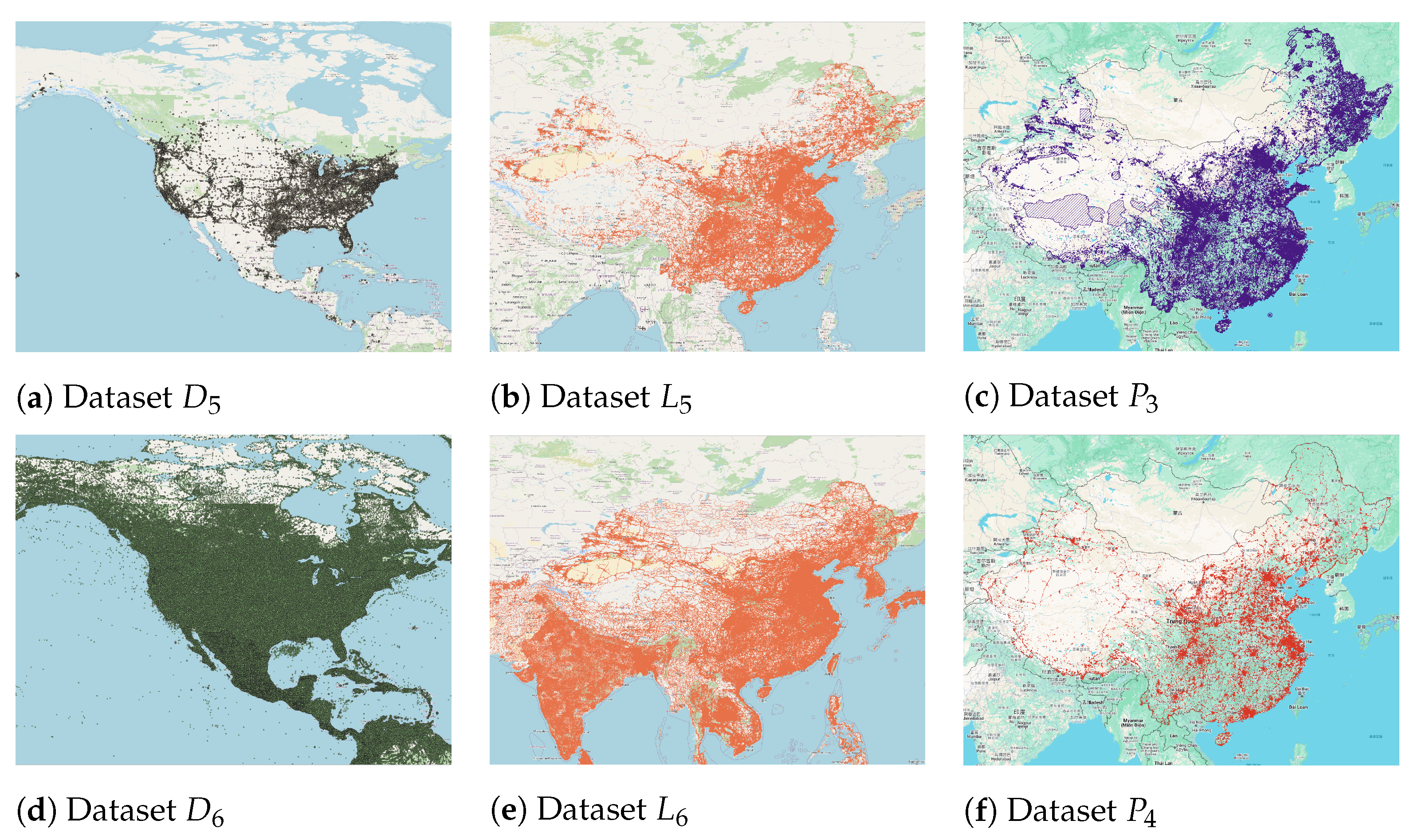
lists the geographic vector points and linestring and polygon feature datasets used in the experiments. The sources of the experimental data include the open-source web map service platform OpenStreetMap and the open-source geographic vector dataset UCR-Star [26]. The sizes of the selected experimental datasets range from thousands to tens of millions points, and all the data are real and randomly distributed. Before the experiments, we preprocessed the data, filtered out invalid data, and unified the reference coordinate system to WGS84 (EPSG:4326). The range of the data is represented by the minimum longitude, minimum latitude, maximum longitude, and maximum latitude of the data points in the sequence. 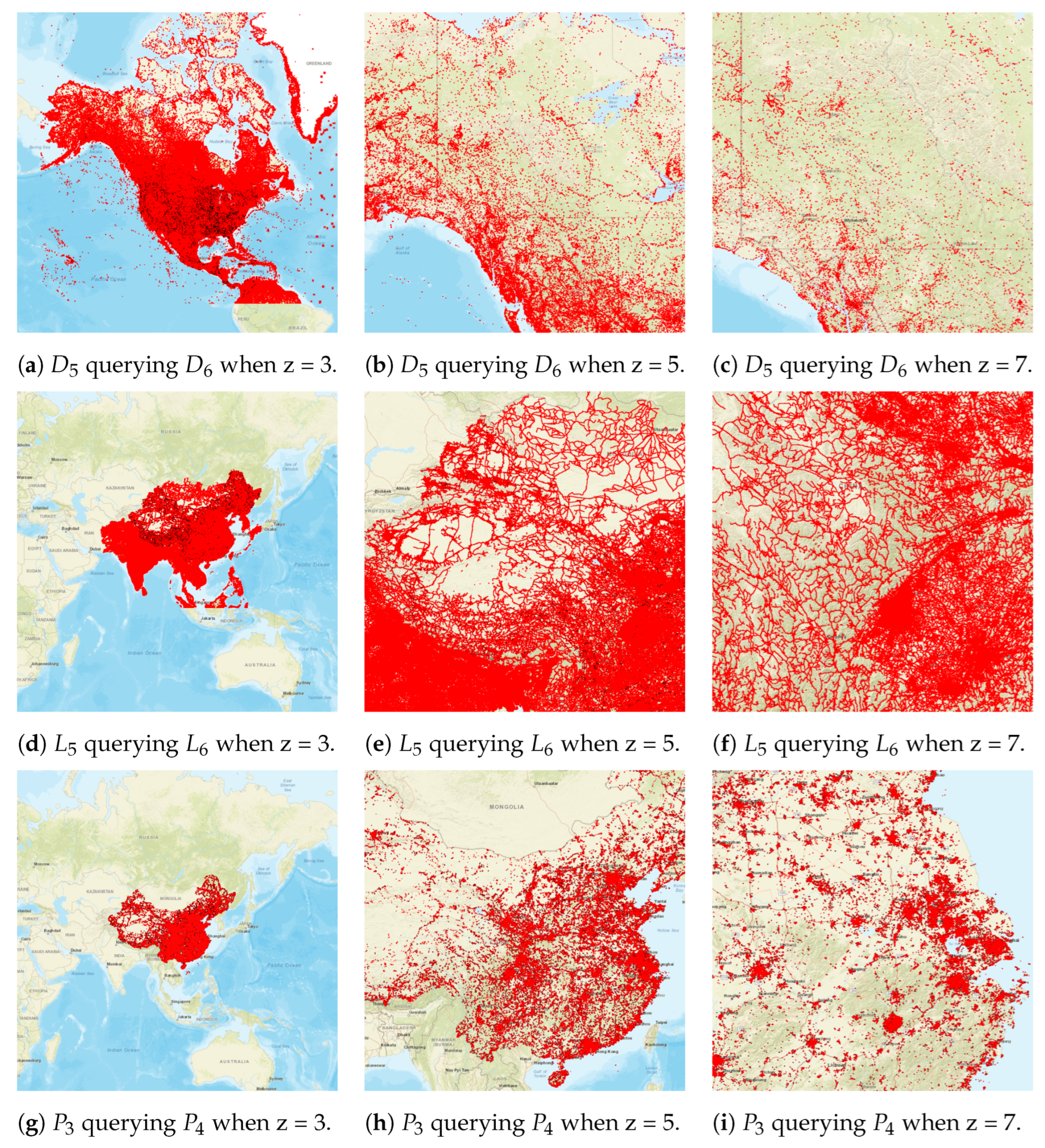As shown in Figure 9, we visualized some of the datasets to intuitively understand the data’s distribution and range.

In both the aforementioned experiments with PixelQuery, the tasks are carried out for each pixel independently, utilizing a multi-process message passing framework (MPI) along with OpenMP for parallel processing to enhance the effectiveness of queries and final visualizations. In the two experiments described below, 32 MPI processes were performed at once, with each MPI process comprising four OpenMP threads.

4.1. Experiment 1: The Effect of Adjustable Parameter n

Given that the sampling number n is an adjustable parameter in this algorithm, to evaluate its impact on the algorithm’s accuracy and speed, we set the sampling numbers to 3, 10, and 20, respectively. To ensure the stability and reliability of the algorithm, we conducted 100 algorithm experiments for each different n and then obtained the average values of the algorithm’s execution time and accuracy rate. The accuracy rate of PixelQuery can be obtained by comparing whether the visualization results of PixelQuery and the data-driven method are the same at the pixel level. We define this accuracy rate as consistency, and the calculation method we used for consistency is as follows:

$$Consistency={\displaystyle \frac{pixe{l}_{consistent}}{pixe{l}_{invovled}}}$$

(2)

$pixe{l}_{consistent}$ refers to the number of pixels in which the visual results of PixelQuery and the data-driven method are identical, while $pixe{l}_{involved}$ denotes the number of pixels involved in the query in which $t_v$s are being detected. Pixels not containing $t_v$s are filtered out to avoid an artificially inflated accuracy rate. The accuracy of each pixel is calculated separately.

We selected point datasets $D_5$ and $D_6$, linestring datasets $L_5$ and $L_6$, and polygon datasets $P_3$ and $P_4$. The zoom range was set from 3 to 7, and $R_B$ was set to 500, 1000, and 5000 m. The selected datasets cover three types of vector objects. They contain a large volume of data, which are unevenly distributed and span a wide range. The experimental results obtained from multiple resolutions and query radii are representative.

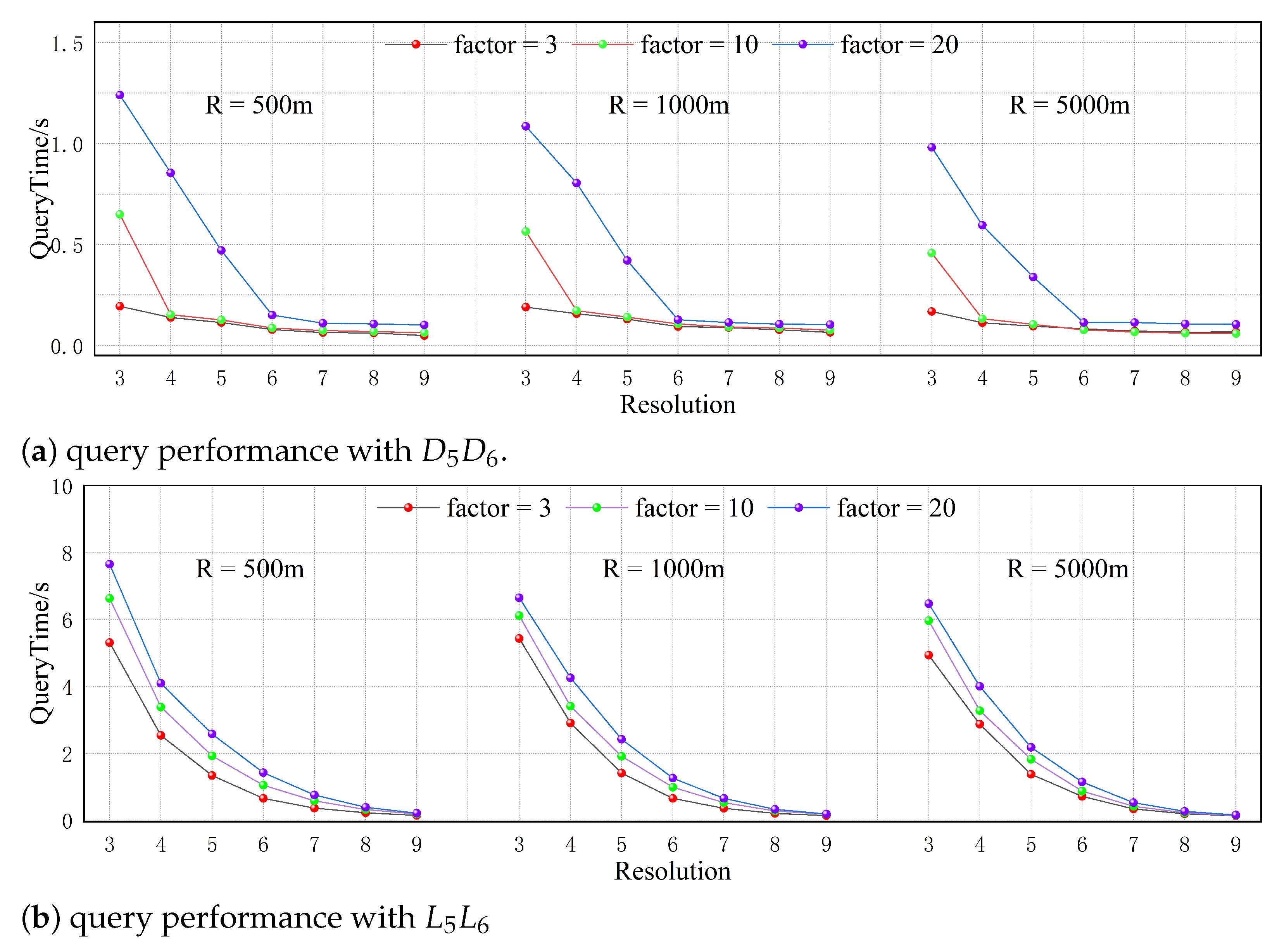
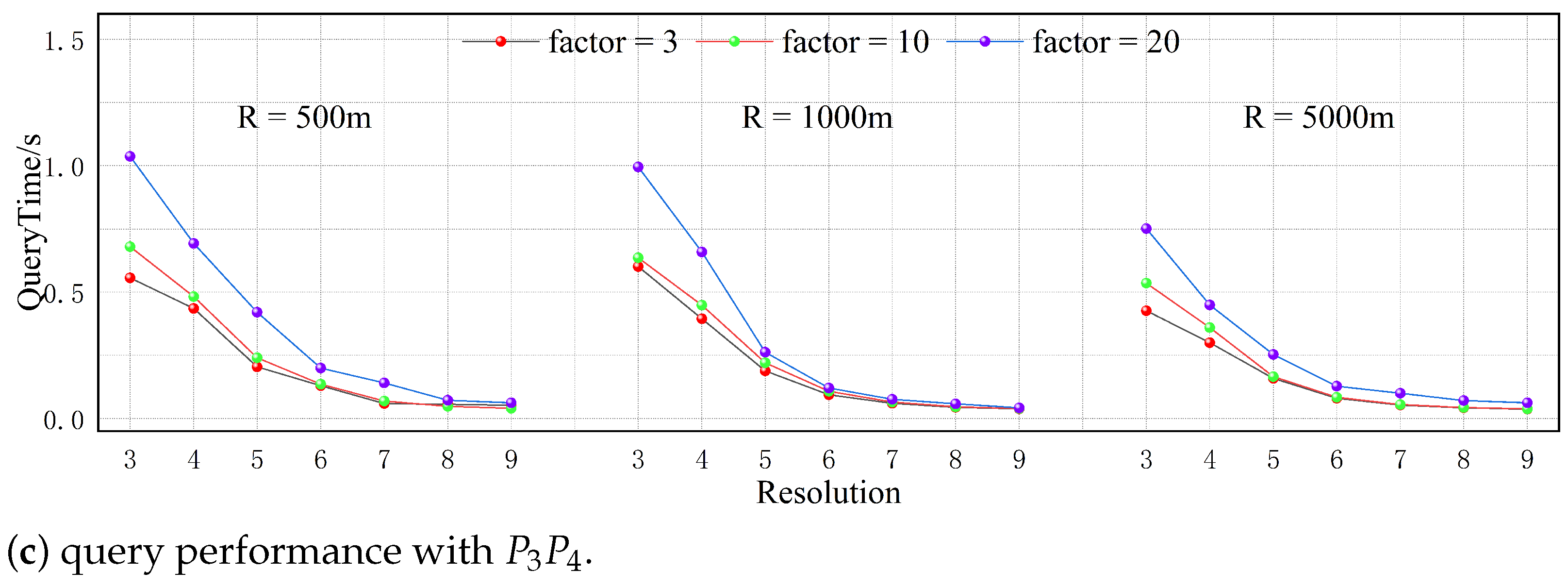
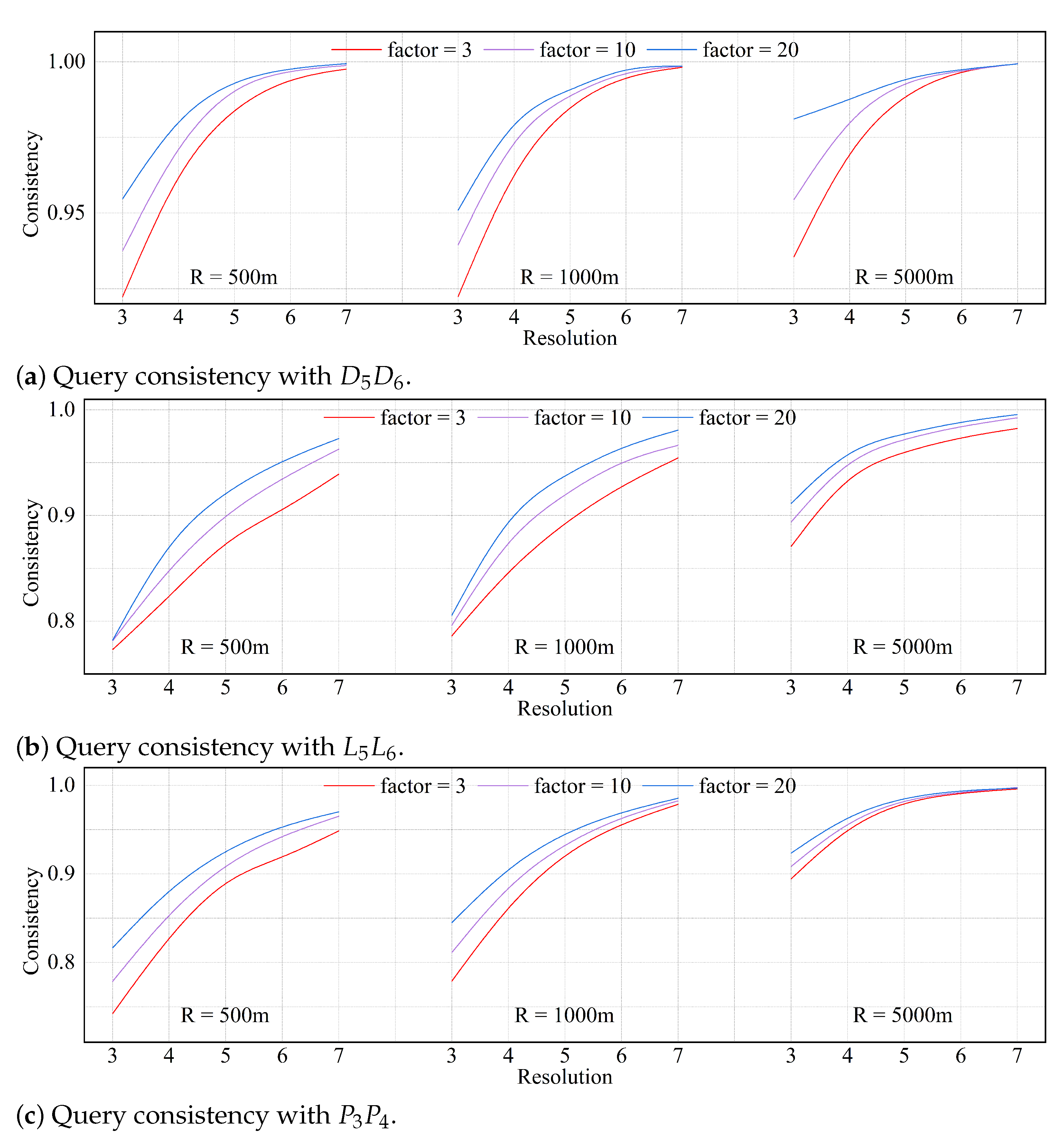
In Figure 10 and Figure 11, the horizontal axis represents the resolution size. Curves of different colors represent different values of n, and the vertical axes represent the average consistency of different pixels at each resolution and the average running time of the algorithm, respectively. By analyzing Figure 10 and Figure 11, it can be observed that as n increases, the consistency of the algorithm under different conditions shows an upward trend. It can be said that the number of sampling times n determines the accuracy of the query visualization results of PixelQuery. However, significant diminishing returns are observed when the number of sampling points exceeds a certain threshold. When n increases from 3 to 10, the recall rates at zoom level 3 improve by approximately 1.6%, 0.7%, and 2.3%, respectively. When n continues to increase from 10 to 20, the recall rates are further improved by 2.2%, 1%, and 2.9%. However, the average query times increase by 99.4%, 10.8%, and 52.5%, respectively.

When comparing n = 20 with n = 10 in all situations, the average consistency increases by only 0.44%, 0.92%, and 0.97% across different datasets. Concurrently, the average query time increases by 11.3%, 18.8%, and 55.1%. When n is set to the total number of $t_v$s that actually meet the conditions within a pixel, the algorithm’s consistency will reach 100%, but this will also significantly increase its processing time. Therefore, reasonably controlling the value of n is crucial to take advantage of the utility of PixelQuery.

Based on the analysis above, it can be concluded that when the number of n is reasonable, the accuracy of PixelQuery can be kept within an acceptable range. To ensure the controllability of the experiment, this study set the number of n to 20 for subsequent experiments. This value was chosen because it maintains an average consistency of 94.7% (and a minimum 80%) while still providing satisfactory query responsiveness. From the above experiments, it can also be concluded that PixelQuery has excellent processing efficiency with different types of large-scale datasets.

4.2. Experiment 2: Outperforming Data-Driven Methods

This experiment compares four leading spatial databases and commercial softwares: QGIS, ArcGIS, PostgreSQL, and Sedona. In this experiment, the resolution of the visualization window for PixelQuery was set to 1920 × 1080, with a visualization level of 3. The $R_{d}s$ used in the experiment, $D_1$, $D_3$, $D_5$, $L_1$, and $L_3$, and the $T_{d}s$$D_2$, $D_4$, $D_6$, $L_2$, and $L_4$ demonstrate the increased query performance advantage of the PixelQuery algorithm as the size of the dataset and its spatial range expand. The experiment conducts DRJQ tasks on datasets of the same type but of varying sizes and with different spatial join query radii. In the experiment, spatial indexes were configured for each method. ArcGIS used a grid index, while QGIS, PostgreSQL, and Sedona were all configured using R-tree indexes.

On the same data scale, Sedona outperforms QGIS, PostgreSQL, and ArcGIS. However, when dealing with large-scale geographic vector data queries, the time consumption of all four data-driven methods increases significantly. This is because when a data-driven method addresses the DRJQ problem, it needs to perform query judgments on each feature, and low-performance hardware cannot complete these query operations quickly. Among the four methods, QGIS is less sensitive to the increase in query radius and is more significantly affected by data size; PostgreSQL performs better with smaller data sizes, but its speed is significantly affected by both the data size and query radius. At a data scale of tens of millions of point, the computation times of QGIS and PostgreSQL are much higher than those of ArcGIS and Sedona. This is due to their query method, which relies on spatial indices to perform nearest-neighbor queries between source vector features and neighboring vector features, as the number of queries rapidly increases as the size of the data grows significantly.

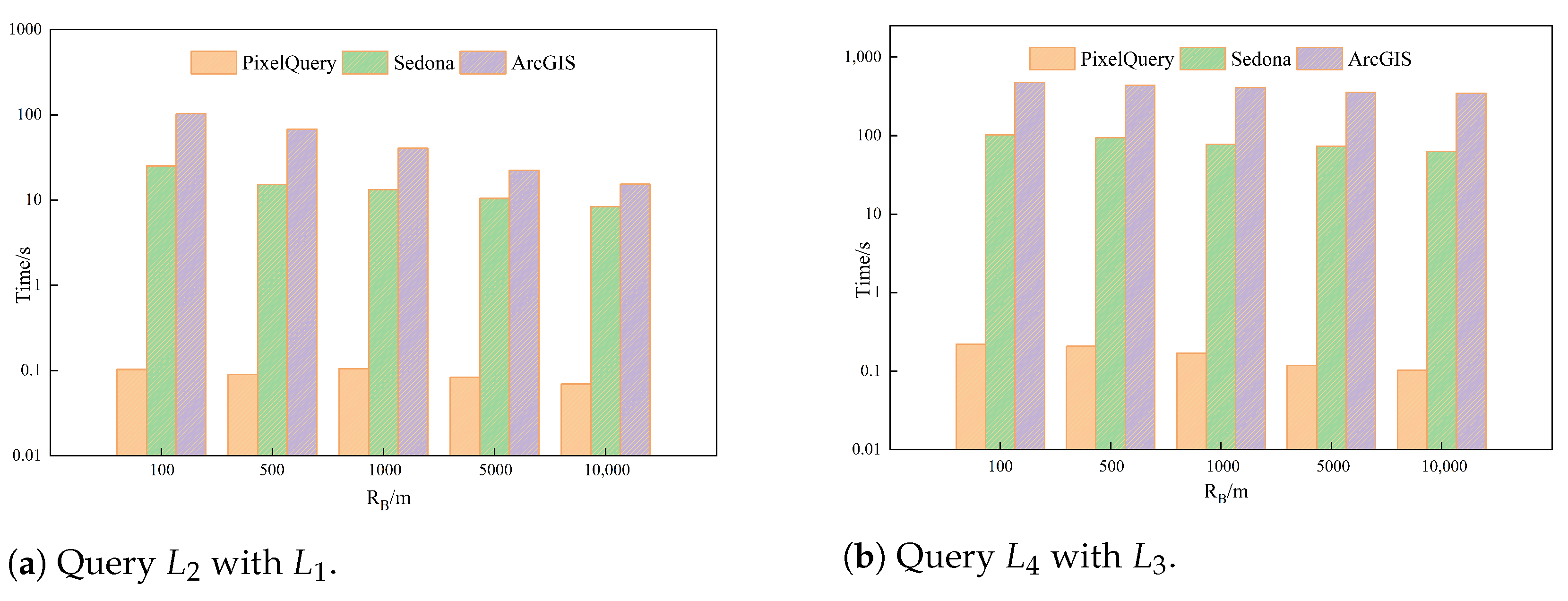
As shown in Figure 12, PixelQuery’s query speed consistently outperformed the four data-driven methods in the experiments with point datasets. Compared to Sedona, which exhibited the best responsiveness among the data-driven methods at different data scales, PixelQuery was 2.69 times, 24 times, and 76.04 times faster than Sedona. As the scale of the data increased, the advantage of PixelQuery became increasingly evident. When performing spatial join queries between line and polygon features, QGIS and PostgreSQL failed to perform queries normally under single-machine conditions. The query times of PixelQuery, ArcGIS, and Sedona are shown in Figure 13a. The query tasks in the figures are as follows: $L_1$ querying $L_2$; $L_3$ querying $L_4$. PixelQuery also demonstrated a superior speed in query experiments between line features. 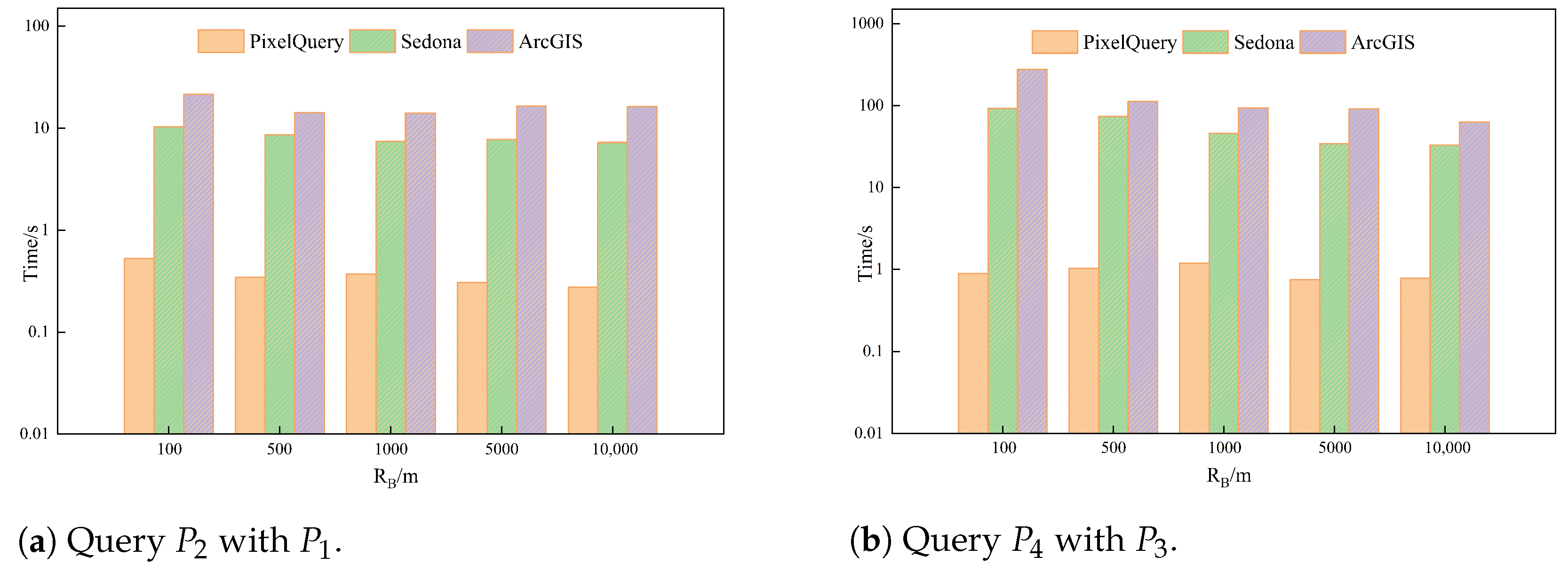In the task of $L_1$ querying $L_2$, PixelQuery’s running time was 2.6% that of Sedona’s. For larger-scale and more widely distributed datasets, such as L3 and L4, this gap widened to 0.328%. In the experimental query of polygon data types, PixelQuery also demonstrated an excellent query speed. As shown in Figure 13b, we conducted queries with different Rb values in two groups of datasets: $P_1$ with $P_2$ and $P_3$ with $P_4$. The results showed that the query time of PixelQuery was only 4.41% and 5.66% that of Sedona.

As shown in Figure 14, the slowest computation time of PixelQuery across the various experiments is 1.29 s, with its query performance showing minimal fluctuations under varying query conditions. The experimental results show that PixelQuery performs well on all data types and under all query conditions, especially on high-density datasets.

5. Discussion

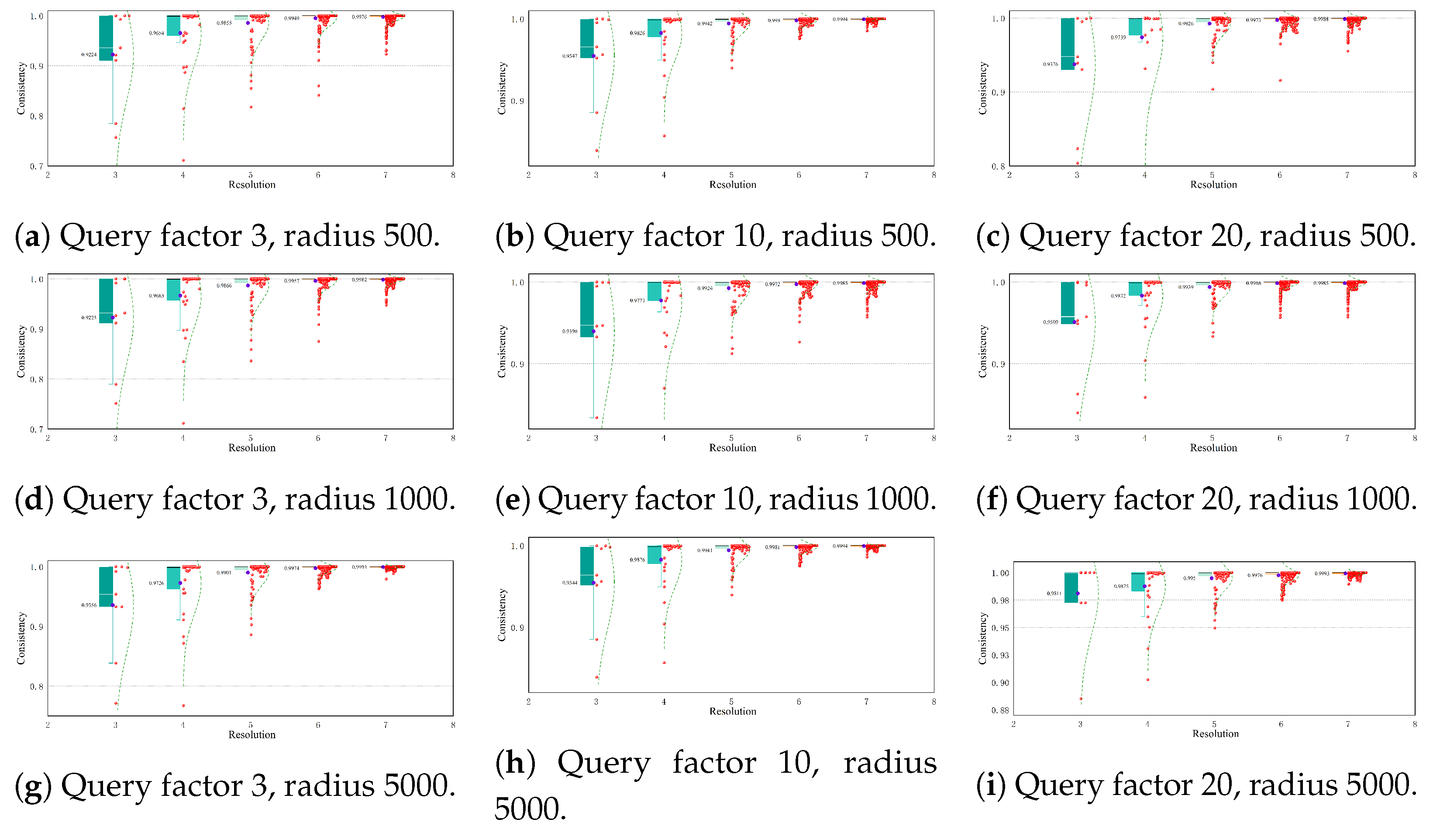
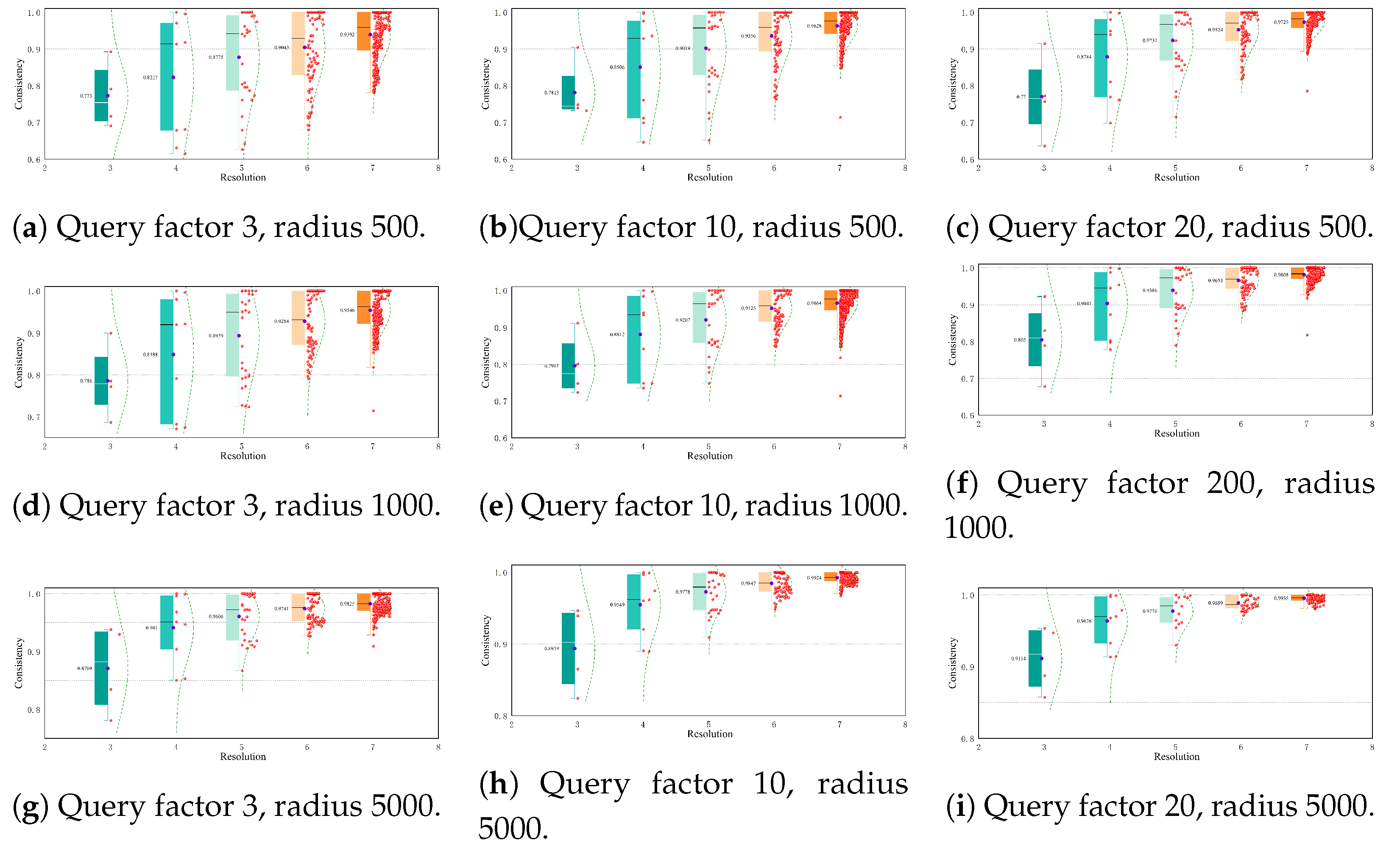
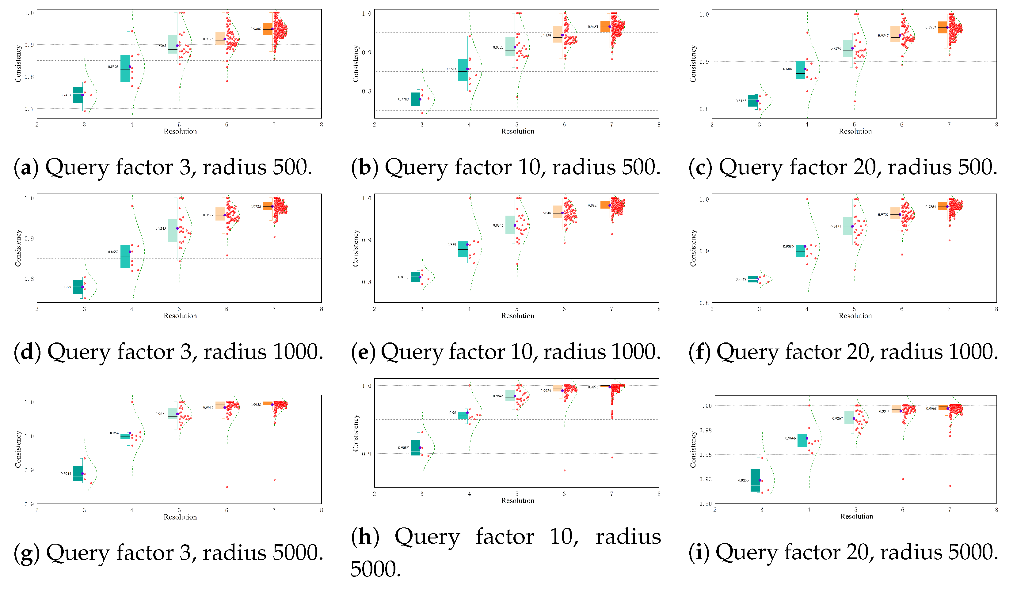
In this chapter, we conduct a detailed analysis of the data from Experiment 1. We recorded the consistency of each pixel under different resolutions and analyzed the performance of PixelQuery in conjunction with the visualization results. Figure 15 presents the visualization results of this experiment, where red pixels indicate identical query results and black pixels represent opposing query results. The visualization reveals that regions with a higher density of black pixels correspond to areas with a sparse distribution of vector features. As the resolution increases, the probability of correct queries being within the query factor threshold also increases, thus enhancing consistency.

Figure 16, Figure 17 and Figure 18 show the influence of the parameter n on the consistency index when different datasets and query conditions are used. Here, the horizontal axis represents the resolution and the vertical axis represents the consistency. The red scatter points are used to represent the accuracy of each pixel at the same resolution. It should be noted that there is an exponential growth relationship between the number of pixels and the resolution. The box of the half-boxplot is defined by the lower quartile and the upper quartile. This interval covers 50% of the middle samples in the dataset and can effectively reflect the central tendency and distribution range of the data. In addition, the curve drawn on the right side of the box is a normal distribution curve which is fitted based on the pixel accuracy data. This curve helps us to intuitively judge the distribution of and changing trends in the pixel accuracy data.

At lower zoom levels, the consistency of pixels within a sparse data distribution is relatively poor, and there is a large gap in the accuracy rate among pixels. However, as the zoom level increases, the boxes gradually become narrower and approach 1, which means that the consistency of each pixel gradually improves and the distribution becomes more concentrated. When the resolution is 7, the accuracy rate of most pixels reaches 1. Similarly, at the same resolution, increasing the values of n and $R_B$ can also improve the consistency to a certain extent and accelerate the speed at which the consistency reaches 1.

This phenomenon occurs because at lower resolutions the spatial extent of each pixel is larger and the number of spatial vectors contained within each pixel increases significantly. However, when the data distribution is sparse, the number of $t_v$s that meet the query conditions is lower. In such cases, when the value of n is small, the probability of randomly sampling and finding a $t_v$ that may satisfy the query conditions decreases. This may lead to situations where the pixel visualization results are correct, but the algorithm judges them incorrectly. To reduce the probability of such misjudgments, it is necessary to appropriately increase the value of n or expand the query radius, as shown in Figure 19.

Based on the above analysis and discussion, it can be concluded that the algorithm proposed in this paper overcomes the shortcoming of traditional data-driven methods in their slow processing of DRJQ tasks in large-scale vector datasets. It greatly improves query efficiency and maintains high accuracy. It achieves rapid responses with different types and scales of data. However, this research still has some limitations:

1. In the scenario of low-resolution sparse data, our algorithm’s query accuracy rate is relatively low. 2. The setting of the influence factor n is based on experimental experience and cannot be adaptively adjusted according to the input data.

The following are some research directions for its optimization in future work: 1. Adopt a sampling method that takes into account contextual influence. Consider the impact of the order of sampling points within the same pixel. Reduce the probability of sampling the next point for sampling points that do not meet the conditions and increase the probability of sampling of other candidate points far from this point. This could help the algorithm effectively traverse the entire spatial range of the pixel quickly.

2. Create an adaptive adjustment strategy for the influence factor n. Combine methods such as resolution, query radius, and data distribution for sampling estimation and regional division to adaptively adjust the value of n and achieve a faster and more accurate query performance.

6. Conclusions

This paper presents PixelQuery, an efficient pixel-level computation method used for DRJQs in large-scale geographic vector data. It achieves efficient interactive visualization using a visualization-oriented strategy. Beyond its technical contributions to the field, PixelQuery demonstrates transformative potential in practical domains. For instance, in urban disaster response, its rapid query capabilities enable the dynamic mapping of risk areas in emergencies. In real-time traffic monitoring, it can quickly visualize congestion patterns without the need to resolve high-performance hardware bottlenecks. The robustness of PixelQuery is verified through experiments on heterogeneous datasets. It achieves a consistent performance (1.29–7.64 s) on a standard laptop without the need for partitioning specific datasets. Notably, in test scenarios, its pixel-based approach reduces its computational overhead by 62.8–99.6% compared to traditional geometric methods, making it particularly suitable for large-scale data query tasks under resource-constrained conditions.

In summary, the proposed algorithm bridges the gap between large-scale geospatial analysis and hardware performance, enabling the efficient completion of DRJQ tasks across various scenarios. This advancement contributes to the development of GISs, urban planning, and environmental monitoring by providing a scalable and computationally efficient solution for efficient spatial data processing.

References

- OpenStreetMap. OpenStreetMap. Available online: https://www.openstreetmap.org/ (accessed on 14 April 2025).
- Mella, E.; Rodríguez, M.A.; Bravo, L.; Gatica, D. Query Rewriting for Semantic Query Optimization in Spatial Databases. Geoinformatica 2019, 23, 79–104. [Google Scholar] [CrossRef]
- Wang, H.; Liu, L.; Wang, J.; Gao, Y. Data Optimization for Spatial Data Mining and Classification in Marine Geochemical Exploration. In Proceedings of the 11th International Conference on Modelling, Identification and Control (ICMIC2019), Tianjin, China, 13–15 July 2019; Wang, R., Chen, Z., Zhang, W., Zhu, Q., Eds.; Springer Singapore: Singapore, 2020; Volume 582, pp. 1261–1270. [Google Scholar] [CrossRef]
- Zhu, L.; Yu, W.; Zhang, C.; Zhang, Z.; Huang, F.; Yu, H. SVS-JOIN: Efficient Spatial Visual Similarity Join for Geo-Multimedia. IEEE Access 2019, 7, 158389–158408. [Google Scholar] [CrossRef]
- García-García, F.; Corral, A.; Iribarne, L.; Vassilakopoulos, M.; Manolopoulos, Y. Efficient Distance Join Query Processing in Distributed Spatial Data Management Systems. Inf. Sci. 2020, 512, 985–1008. [Google Scholar] [CrossRef]
- Eldawy, A.; Mokbel, M.F. SpatialHadoop: A MapReduce Framework for Spatial Data. In Proceedings of the 2015 IEEE 31st International Conference on Data Engineering, Seoul, Republic of Korea, 13–17 April 2015; pp. 1352–1363. [Google Scholar] [CrossRef]
- Zaharia, M.; Chowdhury, M.; Das, T.; Dave, A.; Ma, J.; McCauly, M.; Franklin, M.J.; Shenker, S.; Stoica, I. Resilient Distributed Datasets: A {fault-Tolerant} Abstraction for {in-Memory} Cluster Computing. In Proceedings of the 9th USENIX Symposium on Networked Systems Design and Implementation (NSDI 12), San Jose, CA, USA, 25–27 April 2012; pp. 15–28. [Google Scholar]
- Tang, M.; Yu, Y.; Mahmood, A.R.; Malluhi, Q.M.; Ouzzani, M.; Aref, W.G. LocationSpark: In-memory Distributed Spatial Query Processing and Optimization. Front. Big Data 2020, 3, 30. [Google Scholar] [CrossRef] [PubMed]
- Vu, T.; Belussi, A.; Migliorini, S.; Eldawy, A. A Learning-Based Framework for Spatial Join Processing: Estimation, Optimization and Tuning. VLDB J. 2024, 33, 1155–1177. [Google Scholar] [CrossRef]
- De Bernardo, G.; Penabad, M.R.; Corral, A.; Brisaboa, N.R. Classic Distance Join Queries Using Compact Data Structures. Inf. Sci. 2024, 674, 120732. [Google Scholar] [CrossRef]
- Moutafis, P.; Mavrommatis, G.; Vassilakopoulos, M.; Sioutas, S. Efficient Processing of All-k-Nearest-Neighbor Queries in the MapReduce Programming Framework. Data Knowl. Eng. 2019, 121, 42–70. [Google Scholar] [CrossRef]
- Kim, W.; Kim, Y.; Shim, K. Parallel Computation of K-Nearest Neighbor Joins Using MapReduce. In Proceedings of the 2016 IEEE International Conference on Big Data (Big Data), Washington, DC, USA, 5–8 December 2016; pp. 696–705. [Google Scholar] [CrossRef]
- Lu, W.; Shen, Y.; Chen, S.; Ooi, B.C. Efficient Processing of k Nearest Neighbor Joins Using MapReduce. arXiv 2012. arXiv:cs/1207.0141. [Google Scholar] [CrossRef]
- Akdogan, A.; Demiryurek, U.; Banaei-Kashani, F.; Shahabi, C. Voronoi-Based Geospatial Query Processing with MapReduce. In Proceedings of the 2010 IEEE Second International Conference on Cloud Computing Technology and Science, Indianapolis, IN, USA, 30 November–3 December 2010; pp. 9–16. [Google Scholar] [CrossRef]
- Zhang, C.; Li, F.; Jestes, J. Efficient Parallel kNN Joins for Large Data in MapReduce. In Proceedings of the 15th International Conference on Extending Database Technology, Berlin, Germany, 27–30 March 2012; pp. 38–49. [Google Scholar] [CrossRef]
- Corral, A.; Manolopoulos, Y.; Theodoridis, Y.; Vassilakopoulos, M. Algorithms for Processing K-Closest Queries spatial Databases. Data Knowl. Eng. 2004, 49, 67–104. [Google Scholar] [CrossRef]
- Kim, Y.J.; Patel, J. Performance Comparison of the \rm R⌃\ast-Tree and the Quadtree for kNN and Distance Join Queries. IEEE Trans. Knowl. Data Eng. 2010, 22, 1014–1027. [Google Scholar] [CrossRef]
- Roumelis, G.; Vassilakopoulos, M.; Corral, A.; Manolopoulos, Y. Efficient Query Processing on Large Spatial Databases: A Performance Study. J. Syst. Softw. 2017, 132, 165–185. [Google Scholar] [CrossRef]
- Guttman, A. R-Trees: A Dynamic Index Structure for Spatial Searching. In Proceedings of the 1984 ACM SIGMOD International Conference on Management of Data—SIGMOD ’84, Boston, MA, USA, 18–21 June 1984; p. 47. [Google Scholar] [CrossRef]
- Belussi, A.; Migliorini, S.; Eldawy, A. Cost Estimation of Spatial Join in Spatialhadoop. Geoinformatica 2020, 24, 1021–1059. [Google Scholar] [CrossRef]
- García-García, F.; Corral, A.; Iribarne, L.; Vassilakopoulos, M. Efficient Distributed Algorithms for Distance Join Queries in Spark-Based Spatial Analytics Systems. Int. J. Gen. Syst. 2023, 52, 206–250. [Google Scholar] [CrossRef]
- Ma, M.; Yang, A.; Wu, Y.; Chen, L.; Li, J.; Jing, N. DiSA: A Display-Driven Spatial Analysis Framework for Large-Scale Vector Data. In Proceedings of the 28th International Conference on Advances in Geographic Information Systems, Seattle, WA, USA, 3–6 November 2020; pp. 147–150. [Google Scholar] [CrossRef]
- Liu, Z.; Chen, L.; Yang, A.; Ma, M.; Cao, J. HiIndex: An Efficient Spatial Index for Rapid Visualization of Large-Scale Geographic Vector Data. ISPRS Int. J. Geo-Inf. 2021, 10, 647. [Google Scholar] [CrossRef]
- Ma, M.; Wu, Y.; Ouyang, X.; Chen, L.; Li, J.; Jing, N. HiVision: Rapid Visualization of Large-Scale Spatial Vector Data. Comput. Geosci. 2021, 147, 104665. [Google Scholar] [CrossRef]
- Chen, L.; Liu, Z.; Ma, M. Interactive Visualization of Geographic Vector Big Data Based on Viewport Generalization Model. Appl. Sci. 2022, 12, 7710. [Google Scholar] [CrossRef]
- Ghosh, S.; Vu, T.; Eskandari, M.A.; Eldawy, A. UCR-STAR: The UCR Spatio-Temporal Active Repository. SIGSPATIAL Spec. 2019, 11, 34–40. [Google Scholar] [CrossRef]
Figure 1.
The query visualization processing flow used in PixelQuery.
Figure 2.
Model of visualization-oriented DRJQ.
Figure 3.
Illustrations of different intersecting pixel P with radius R.
Figure 4.
Illustrations of different not intersecting pixel P with radius R.
Figure 5.
The query regions of different objects with distance threshold .
Figure 6.
The bounding boxes used to solve the DRJQ.
Figure 7.
The processing flow of the visualization-oriented DRJQ algorithm.
Figure 8.
The impact of the query factor on the query results.
Figure 9.
Visualization of partial datasets.
Figure 10.
Query speed results.
Figure 11.
The query consistency results.
Figure 12.
The query performance comparison of our algorithm with data-driven methods.
Figure 13.
The query performance comparison of our algorithm with ArcGIS and Sedona on linestring datasets.
Figure 14.
The query performance comparison of our algorithm with ArcGIS and Sedona on polygon datasets.
Figure 15.
The visualization of the consistency experiment with a query factor = 20 and = 5000 m.
Figure 16.
The consistency experiment of querying .
Figure 17.
Figure 18.
Figure 19.
The impact of the value of n on the query results.