

RouteLAND: An Integrated Method and a Geoprocessing Tool for Characterizing the Dynamic Visual Landscape Along Highways


Abstract
1. Introduction
2. Background and Related Work
2.1. Describing the Perceived Size of Landscape Elements from the Egocentric (Human) Perspective: Concepts and Issues
2.2. Describing the Dynamic Landscape Along Higways: Concepts and Issues
3. Materials and Methods
3.1. Overall Rationale
3.2. Input Data (Case Study)
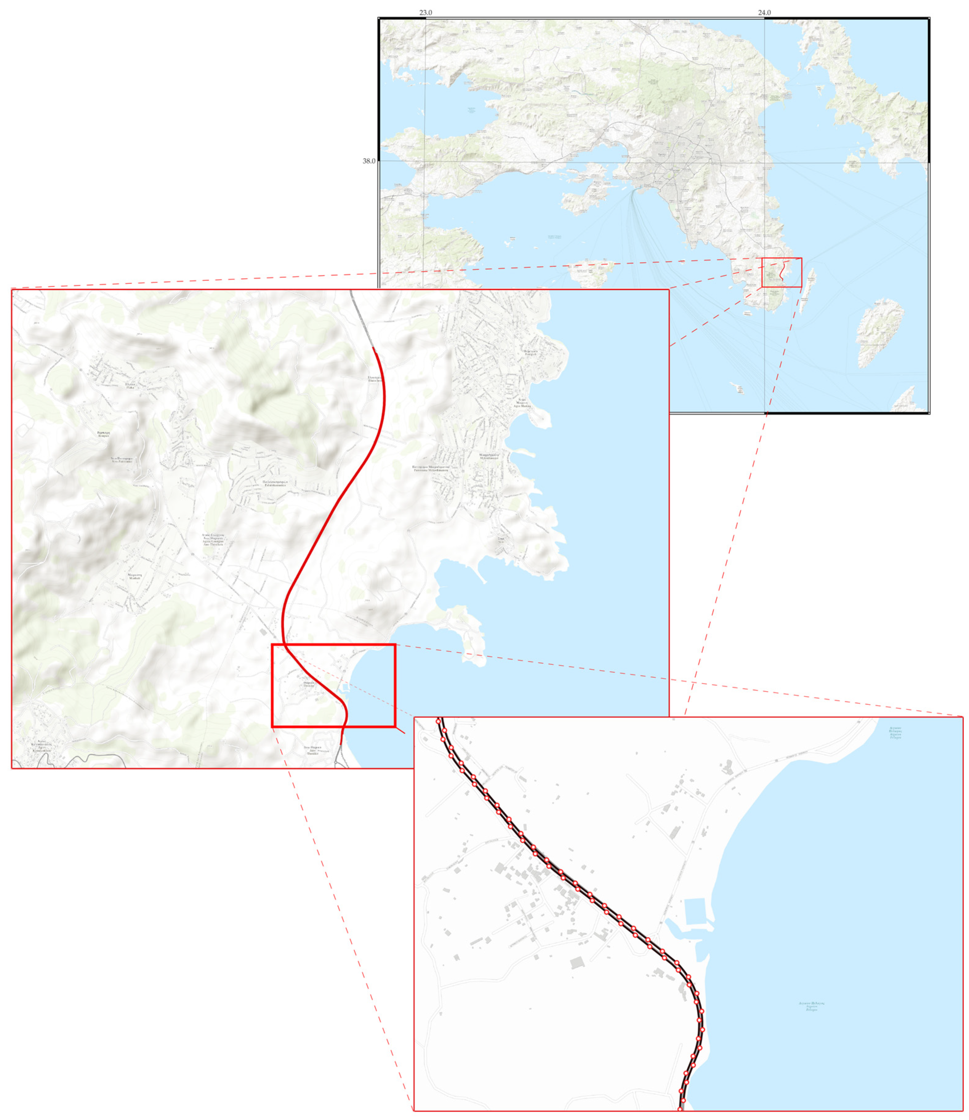
3.3. Study Area
3.4. Methodology
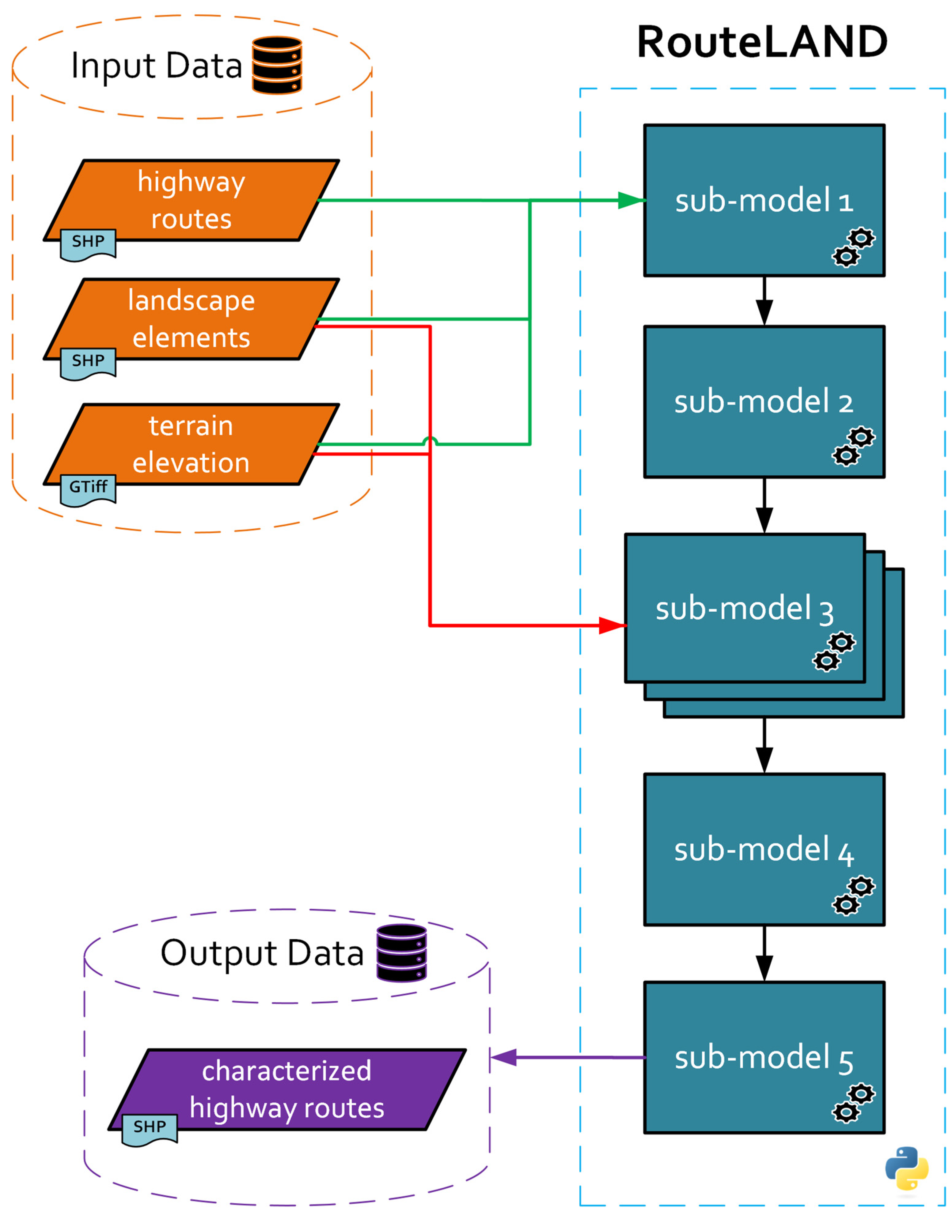
3.4.1. Overview
- Sub-model 1: Generation of viewpoints along highway routes and computation of route segments’ viewing directions;
- Sub-model 2: Computation of (start and end) horizontal viewing directions based on the route segments’ mean viewing directions and speed limits (max speed) for further viewshed analyses computation;
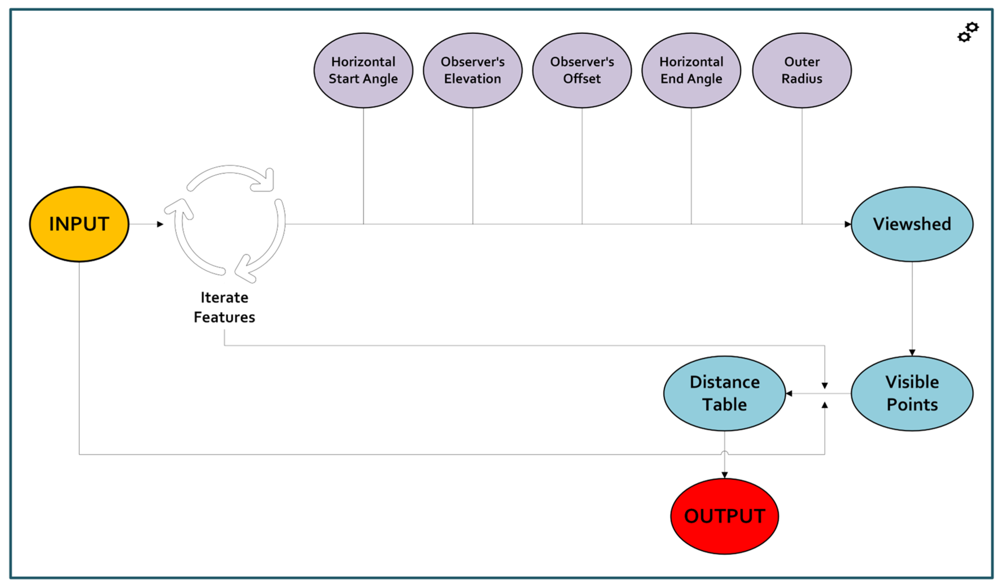
- Sub-model 3: Iterative computation of viewsheds and other relationships or attributes (distance, elevation, slope, aspect, LU/LC) of the visible/viewshed cells (or points) associated with each respective viewpoint;
- Sub-model 4: Computation of viewing significance and actual landscape composition, at the level of the highway route’s viewpoints dFoV, based on the spatial/thematic relationships and analyses among the viewshed points’ attributes and the associated viewpoints’ positions;
- Sub-model 5: Qualitative and quantitative characterization of the highway routes regarding the dominant landscape element ‘occupying’ the dFoV per route segment (Figure 2).
3.4.2. Method Development: Rationale and Computations (Geoprocesses and Calculations)
- if st_angle < 0°: °;
- else if 0° <= st_angle <= 360°: °;
- else (if st_angle > 360°): °;if end_angle < 0°: °;
- else if 0° <= end_angle <= 360°: °;
- else (if end_angle > 360°): °;

| Speed Limit (km/h) | Horizontal Angle (°) | Horizontal Half-Angle (°) |
|---|---|---|
| 0 | 120 | 60 |
| 0 < sl <= 30 | 110 | 55 |
| 30 < sl <= 65 | 100 | 50 |
| 65 < sl <= 80 | 60 | 30 |
| 80 < sl <= 100 | 40 | 20 |
| >100 | 20 | 10 |
- For the calculation of PAVA, several individual physical quantities were calculated:
- The vertical (positive/negative) viewing angle (VerAng) at which each viewpoint of the route is connected to each viewshed point of the cloud (sharing a common FID) was calculated as a function of the viewpoint elevation (VPElev), viewshed elevation (ELEV), and horizontal distance among viewpoint and viewshed points (NEAR_DIST), which is defined as follows:
- The actual (i.e., not just horizontal) distance (ActDist) from each viewpoint of the route to each viewshed point of the cloud (sharing a common FID) was also calculated as a function of the viewpoint elevation (VPElev), viewshed elevation (ELEV), and horizontal distance among viewpoint and viewshed points (NEAR_DIST), which is defined in the following:
- The relative vertical viewing angle (RelVAng) that occurs between (i) the vertical angle at which each viewpoint of the route is connected to each viewshed point of the cloud (VerAng) and (ii) the slope of the surface of the viewshed cells (SLOPE), which is calculated as follows:
- The actual height (ActHei)—due to the relative viewing vertical angle—of each viewshed cell of the cloud relative to each viewpoint of the route (sharing a common FID), which is herein computed as follows:
- The perceived adjusted vertical viewing angle (PAVA) as a function of ActHei (Equation (6)) and ActDist (Equation (4)), which is based on the following formula:
- On the other hand, for the calculation of PAHA, the following calculations took place:
- The relative horizontal viewing angle (RelHorAng) that occurs between the following: (i) the horizontal angle (azimuth) at which each viewpoint of the route is connected to each viewshed point of the cloud (NEAR_ANGLE) and (ii) the aspect of the surface of the viewshed cells calculated under certain conditions in two stages (a, b):
- (a)
- In order to delimit the relative horizontal viewing angles within the [0–180] range, the following condition was enforced, obtaining the following two arguments (NEAR ANGLE and ASPECT): if ASPECT = = −1 (flat surface): °,else if 0 <= ASPECT <= 180°: ,else (if ASPECT > 180°): ;and then an intermediate variable, RelHorA, was calculated as a function of the two arguments:
- (b)
- In order to delimit the relative horizontal viewing angles within the [0–90] range, the following condition was enforced:if RelHorA <= 90°: RelHorA remains unchanged;else (if RelHorA > 90°): °;and, so:
- The actual width (ActWid)—due to the relative viewing horizontal angle—of each viewshed cell of the cloud relative to each viewpoint of the route (sharing a common FID) was computed using the following equation:
- The perceived adjusted horizontal viewing angle (PAHA) as a function of ActWid (Equation (10)) and ActDist (Equation (4)) was calculated based on the following formula:
PAVA and PAHA indices measure the perceived angular sizes of visible/viewshed cells in the two (vertical and horizontal) dimensions, i.e., perceived angular height and width, while their angle values range in the interval [0, 180)°. The Perceived Visual Significance Index (PerVSI) is a compound index that measures the two-dimensional (solid) angle (measured in square degrees) and occurs as the product of PAVA and PAHA, namely,
3.4.3. Tool Implementation: Employing ArcPy Toolboxes, Toolsets, and Tools
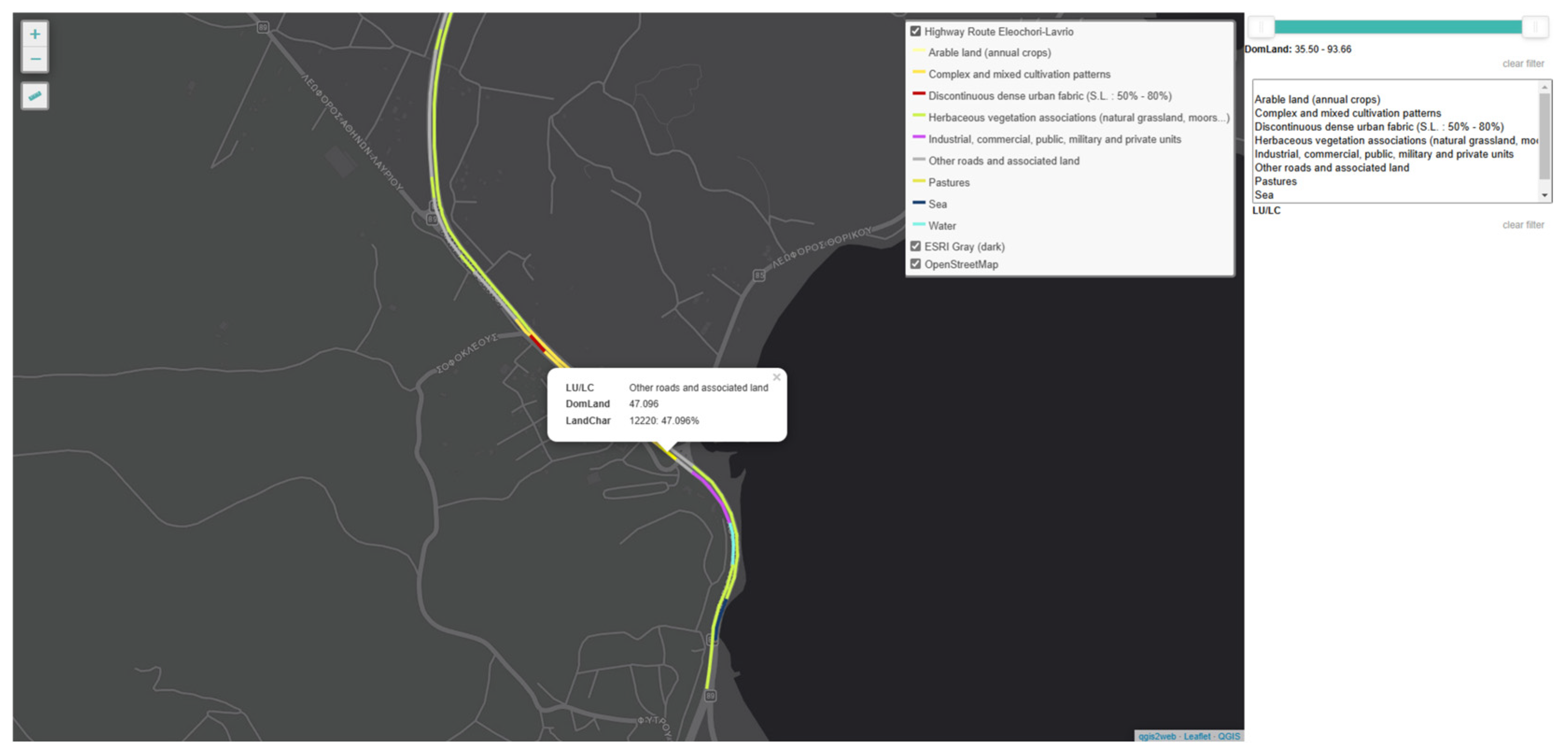
3.4.4. Web Map Design
4. Results
4.1. Presentation
4.2. Evaluation
5. Discussion and Conclusions
5.1. Synopsis
5.2. Assumptions and Limitations
5.3. Future Research and Outlook
Supplementary Materials
Author Contributions
Funding
Data Availability Statement
Conflicts of Interest
References
- Bergen, S.D.; Ulbricht, C.A.; Fridley, J.L.; Ganter, M.A. The Validity of Computer-Generated Graphic Images of Forest Landscape. J. Environ. Psychol. 1995, 15, 135–146. [Google Scholar] [CrossRef]
- Arriaza, M.; Cañas-Ortega, J.F.; Cañas-Madueño, J.A.; Ruiz-Aviles, P. Assessing the Visual Quality of Rural Landscapes. Landsc. Urban Plan. 2004, 69, 115–125. [Google Scholar] [CrossRef]
- Bulut, Z.; Yilmaz, H. Determination of Landscape Beauties through Visual Quality Assessment Method: A Case Study for Kemaliye (Erzincan/Turkey). Environ. Monit. Assess. 2008, 141, 121–129. [Google Scholar] [CrossRef]
- Howley, P.; Donoghue, C.O.; Hynes, S. Landscape and Urban Planning Exploring Public Preferences for Traditional Farming Landscapes. Landsc. Urban Plan. 2012, 104, 66–74. [Google Scholar] [CrossRef]
- López-martínez, F. Visual Landscape Preferences in Mediterranean Areas and Their Socio-Demographic Influences. Ecol. Eng. 2017, 104, 205–215. [Google Scholar] [CrossRef]
- Ulrich, R.S. Human Responses to Vegetation and Landscapes. Landsc. Urban Plan. 1986, 13, 29–44. [Google Scholar] [CrossRef]
- Misgav, A. Visual Preference of the Public for Vegetation Groups in Israel. Landsc. Urban Plan. 2000, 48, 143–159. [Google Scholar]
- Han, K.-T. Responses to Six Major Terrestrial Biomes in Terms of Scenic Beauty, Preference, and Restorativeness. Environ. Behav. 2007, 39, 529–556. [Google Scholar] [CrossRef]
- Hammitv, W.E.; Pattersonb, M.E.; Noe, F.P. Identifying and Predicting Visual Preference of Southern Appalachian Forest Recreation Vistas. Landsc. Urban Plan. 1994, 29, 171–183. [Google Scholar] [CrossRef]
- Purcell, A.T.; Lamb, R.J.; Mainardi Peron, E.; Falchero, S. Preference or Preferences for Landscape? J. Environ. Psychol. 1994, 14, 195–209. [Google Scholar] [CrossRef]
- Strumse, E. Perceptual Dimensions in the Visual Preferences for Agrarian Landscapes in Western Norway. J. Environ. Psychol. 1994, 14, 281–292. [Google Scholar]
- Gao, H.; Abu Bakar, S.; Maulan, S.; Yusof, M.J.M.; Mundher, R.; Chen, B. How Highway Landscape Visual Qualities Are Being Studied: A Systematic Literature Review. Land 2024, 13, 431. [Google Scholar] [CrossRef]
- Tempesta, T. The Perception of Agrarian Historical Landscapes: A Study of the Veneto Plain in Italy. Landsc. Urban Plan. 2010, 97, 258–272. [Google Scholar] [CrossRef]
- Forman, R.T.T. Town Ecology: For the Land of Towns and Villages. Landsc. Ecol. 2019, 34, 2209–2211. [Google Scholar] [CrossRef]
- Ulrich, R.S. Visual Landscapes and Psychological Well-Being. Landsc. Res. 1979, 4, 17–23. [Google Scholar]
- Mcmahan, E.A.; Estes, D. The Effect of Contact with Natural Environments on Positive and Negative Affect: A Meta-Analysis. J. Posit. Psychol. 2015, 9760, 1–13. [Google Scholar] [CrossRef]
- Kaplan, S. The Restorative Benefits of Nature: Toward an Integrative Framework. J. Environ. Psychol. 1995, 15, 169–182. [Google Scholar] [CrossRef]
- Gullone, E. The Biophilia Hypothesis and Life in the 21st Century: Increasing Mental Health or Increasing Pathology? J. Happiness Stud. 2000, 1, 293–322. [Google Scholar] [CrossRef]
- Ulrich, R.S.; Simons, R.F.; Losito, B.D.; Fiorito, E.; Miles, M.A.; Zelson, M. Stress Recovery during Exposure to Natural and Urban Environments. J. Environ. Psychol. 1991, 11, 201–230. [Google Scholar] [CrossRef]
- Grinde, B.; Patil, G.G. Biophilia: Does Visual Contact with Nature Impact on Health and Well-Being? Int. J. Environ. Res. Public Health 2009, 6, 2332–2343. [Google Scholar] [CrossRef] [PubMed]
- Ulrich, R.S. Aesthetic and Affective Response to Natural Environment. In Behavior and the Natural Environment; Altman, I., Wohlwill, J.F., Eds.; Springer: Boston, MA, USA, 1983; pp. 85–125. ISBN 978-1-4613-3539-9. [Google Scholar]
- UN Department of Economic and Social Affairs. World Urbanization Prospects; United Nations: New York, NY, USA, 2019; Volume 12, ISBN 9789211483192.
- Franěk, M. Landscape Preference: The Role of Attractiveness and Spatial Openness of the Environment. Behav. Sci. 2023, 13, 666. [Google Scholar] [CrossRef]
- Misthos, L.-M.; Krassanakis, V.; Merlemis, N.; Kesidis, A.L. Modeling the Visual Landscape: A Review on Approaches, Methods and Techniques. Sensors 2023, 23, 8135. [Google Scholar] [CrossRef]
- Aznar-Casanova, J.; Matsushima, E. Interaction between Egocentric and Exocentric Frames of Reference Assessed by Perceptual Constancy Parameters. Cogn. Stud. 2008, 15, 22–37. [Google Scholar]
- Harrower, M.; Sheesley, B. Moving beyond Novelty: Creating Effective 3D Fly-over Maps. In Proceedings of the Anais: 22th International Cartographic Conference Mapping Approaches into a Changing World, A Coruña, Spain, 9–16 July 2005; pp. 9–16. [Google Scholar]
- Misthos, L.-M. Mountainous Landscape Exploration Visualizing Viewshed Changes in Animated Maps; National Technical University of Athens: Zografou, Greece, 2014. [Google Scholar]
- Misthos, L.-M.; Menegaki, M. Identifying Vistas of Increased Visual Impact in Mining Landscapes. In Proceedings of the 6th International Conference on Computer Applications in the Minerals Industries (CAMI 2016), Istanbul, Turkey, 5–7 October 2016. [Google Scholar]
- Misthos, L.M. Development of a Geospatial, Multiparametric Model for Assessing Landscape Impacts from Mining; National Technical University of Athens: Zografou, Greece, 2022. [Google Scholar]
- Kent, R.L. Determining Scenic Quality along Highways: A Cognitive Approach. Landsc. Urban Plan. 1993, 27, 29–45. [Google Scholar] [CrossRef]
- Schirpke, U.; Tasser, E.; Tappeiner, U. Landscape and Urban Planning Predicting Scenic Beauty of Mountain Regions. Landsc. Urban Plan. 2013, 111, 1–12. [Google Scholar] [CrossRef]
- Brabyn, L. Modelling Landscape Experience Using “Experions”. Appl. Geogr. 2015, 62, 210–216. [Google Scholar] [CrossRef]
- Council of Europe. The European Landscape Convention—Firenze, 20X. 2000 (ETS No. 176); Official Text in English; Council of Europe: Strasbourg, France, 2000. [Google Scholar]
- Minelli, A.; Marchesini, I.; Taylor, F.E.; De Rosa, P.; Casagrande, L.; Cenci, M. An Open Source GIS Tool to Quantify the Visual Impact of Wind Turbines and Photovoltaic Panels. Environ. Impact Assess. Rev. 2014, 49, 70–78. [Google Scholar] [CrossRef]
- Nutsford, D.; Reitsma, F.; Pearson, A.L.; Kingham, S. Personalising the Viewshed: Visibility Analysis from the Human Perspective. Appl. Geogr. 2015, 62, 1–7. [Google Scholar] [CrossRef]
- Gibson, J.J. The Ecological Approach to Visual Perception; Classic Edition; Psychology Press: London, UK, 2014. [Google Scholar]
- Jin, X. A Review of Cityscape Research Based on Dynamic Visual Perception. Land 2023, 12, 1229. [Google Scholar] [CrossRef]
- Misthos, L.M.; Nakos, B.; Mitropoulos, V.; Krassanakis, V.; Menegaki, M.; Batzakis, D.V. The Effectiveness of Propagating Viewsheds’ Geovisualization from Topographically Prominent Viewroutes. In Proceedings of the 10th International Congress of the Hellenic Geographical Society, Thessaloniki, Greece, 22–24 October 2014; pp. 22–24. [Google Scholar]
- Misthos, L.-M.; Nakos, B.; Krassanakis, V.; Menegaki, M. The Effect of Topography and Elevation on Viewsheds in Mountain Landscapes Using Geovisualization. Int. J. Cartogr. 2019, 5, 44–66. [Google Scholar] [CrossRef]
- Jaal, Z.; Abdullah, J. User’s Preferences of Highway Landscapes in Malaysia: A Review and Analysis of the Literature. Procedia—Soc. Behav. Sci. 2012, 36, 265–272. [Google Scholar] [CrossRef]
- Jin, X.; Wang, J. ScienceDirect Assessing Linear Urban Landscape from Dynamic Visual Perception Based on Urban Morphology. Front. Archit. Res. 2021, 10, 202–219. [Google Scholar] [CrossRef]
- Dupont, L.; Ooms, K.; Duchowski, A.T.; Antrop, M.; Van Eetvelde, V. Investigating the Visual Exploration of the Rural-Urban Gradient Using Eye-Tracking. Spat. Cogn. Comput. 2017, 17, 65–88. [Google Scholar] [CrossRef]
- Barbu, D.M. Visual Field Evaluation Method Of The Automobile Drivers In Traffic. Ann. Fac. Eng. Hunedoara 2016, 14, 163. [Google Scholar]
- Dharmasena, S.; Edirisooriya, S. Impact of Roadside Landscape to Driving Behaviour; Lessons from Southern Highway, Sri Lanka. Cities People Places Int. J. Urban Environ. 2018, 3, 66. [Google Scholar] [CrossRef]
- Rodrigues, M.; Montañés, C.; Fueyo, N. A Method for the Assessment of the Visual Impact Caused by the Large-Scale Deployment of Renewable-Energy Facilities. Environ. Impact Assess. Rev. 2010, 30, 240–246. [Google Scholar] [CrossRef]
- Menegaki, M.E.; Kaliampakos, D.C. Evaluating Mining Landscape: A Step Forward. Ecol. Eng. 2012, 43, 26–33. [Google Scholar] [CrossRef]
- U.S. Government Printing Office. USDA Forest Service National Forest Landscape Management, Vol. 1: Agriculture Handbook No 434; U.S. Government Printing Office: Washington, DC, USA, 1973.
- Swanwick, C. Landscape Character Assessment: Guidance for England and Scotland; The Countryside Agency and Scottish Natural Heritag: London, UK, 2002. [Google Scholar]
- Tveit, M.; Ode, Å.; Fry, G. Key Concepts in a Framework for Analysing Visual Landscape Character. Landsc. Res. 2006, 31, 229–255. [Google Scholar] [CrossRef]
- Dramstad, W.E.; Tveit, M.S.; Fjellstad, W.J.; Fry, G.L.A. Relationships between Visual Landscape Preferences and Map-Based Indicators of Landscape Structure. Landsc. Urban Plan. 2006, 78, 465–474. [Google Scholar] [CrossRef]
- Palmer, J.F. The Contribution of a GIS-Based Landscape Assessment Model to a Scientifically Rigorous Approach to Visual Impact Assessment. Landsc. Urban Plan. 2019, 189, 80–90. [Google Scholar] [CrossRef]
- Schirpke, U.; Tasser, E.; Lavdas, A.A. Potential of Eye-Tracking Simulation Software for Analyzing Landscape Preferences. PLoS ONE 2022, 17, e0273519. [Google Scholar] [CrossRef] [PubMed]
| Input Dataset (Layer) | Format—Geometry | Open Geospatial Dataset |
|---|---|---|
| highway routes | feature class/shapefile—polyline vector | OSM roads |
| terrain elevation | GeoTIFF—raster | EU-DEM |
| landscape elements | feature class/shapefile—polygon vector | Urban Atlas LU/LC |
| terrain slope * | GeoTIFF—raster | EU-DEM |
| terrain aspect * | GeoTIFF—raster | EU-DEM |
| Max Speed (km/h) | Mean Direction (°) | Half-Angle (°) | Start Angle (°) | End Angle (°) |
|---|---|---|---|---|
| 20 | 355 | 55 | 300 | 50 |
| 20 | 5 | 55 | 310 | 60 |
| 50 | 265 | 50 | 215 | 315 |
| 50 | 95 | 50 | 45 | 145 |
| 70 | 175 | 30 | 145 | 205 |
| 70 | 185 | 30 | 155 | 215 |
| 90 | 85 | 20 | 65 | 105 |
| 90 | 275 | 20 | 255 | 295 |
| 110 | 10 | 10 | 0/360 | 20 |
| 110 | 350 | 10 | 340 | 0/360 |
| Input Layer | Toolbox/Data Access Module—ArcPy Function | Toolset | Tool/Class-Function |
|---|---|---|---|
| 1. Initial highway route (OSM roads); 2. Landscape elements (UrbanAtlas LU/LC); 3. Intermediate highway route | Analysis | Extract | Clip; Select |
| Overlay | Identity; SpatialJoin | ||
| Proximity | GenerateNearTable; Buffer | ||
| Statistics | Statistics (Summary Statistics) | ||
| 1. Initial highway route (OSM roads); 2. Landscape elements (UrbanAtlas LU/LC); 3. Terrain elevation; 4. Terrain slope; 5. Terrain aspect (EU-DEM); 6. Intermediate highway route | Management | Fields | AddField; CalculateField; DeleteField |
| General | Merge | ||
| Generalization | Dissolve | ||
| Features | CopyFeatures; FeatureVerticesToPoints | ||
| Joins | JoinField | ||
| Layers and Table Views | MakeFeatureLayer; SelectLayerByAttribute | ||
| Raster Processing | Clip | ||
| Sampling | GeneratePointsAlongLines | ||
| 1. Initial highway route (OSM roads); 2. Terrain elevation; 3. Terrain slope; 4. Terrain aspect (EU-DEM) | Spatial Analyst | Surface | Aspect; Slope; Viewshed2 |
| Extraction | ExtractMultiValuesToPoints | ||
| 1. Initial highway route (OSM roads); 2. Terrain elevation; 3. Terrain slope; 4. Terrain aspect (EU-DEM) | Conversion | From Raster | RasterToPoint |
| 1. Initial highway route | Spatial Statistics | Measuring Geographic Distributions | DirectionalMean |
| 1. Initial highway route | Classes/Cursors | - | SearchCursor |
| UrbanAtlas LU/LC Type | Area of LU/LC Within the Route’s 6 km Zone (%) | Number of Segments with Dominant LU/LC in Route’s dFoV (%) | Mean/Max DomLand for Each Segment (%) |
|---|---|---|---|
| Arable land (annual crops) | 2.10 | 1.03 | 46.37/46.37 |
| Complex and mixed cultivation patterns | 6.61 | 9.23 | 61.75/88.39 |
| Construction sites | 0.01 | - | - |
| Continuous urban fabric (S.L.: >80%) | 0.29 | - | - |
| Discontinuous dense urban fabric (S.L.: 50–80%) | 2.02 | 0.51 | 62.08/62.08 |
| Discontinuous low-density urban fabric (S.L.: 10–30%) | 0.88 | - | - |
| Discontinuous medium density urban fabric (S.L.: 30–50%) | 2.35 | - | - |
| Discontinuous very-low-density urban fabric (S.L.: <10%) | 0.04 | - | - |
| Forests | 1.45 | - | - |
| Green urban areas | 0.02 | - | - |
| Herbaceous vegetation associations (natural grassland, moors...) | 34.92 | 47.18 | 55.13/86.21 |
| Industrial, commercial, public, military, and private units | 1.47 | 1.54 | 78.67/80.09 |
| Isolated structures | 1.23 | - | - |
| Land without current use | 0.11 | - | - |
| Mineral extraction and dump sites | 0.09 | - | - |
| Open spaces with little or no vegetation (beaches, dunes, bare rocks, glaciers) | 0.01 | - | - |
| Other roads and associated land | 2.74 | 34.36 | 66.12/93.66 |
| Pastures | 3.22 | 4.10 | 41.90/49.15 |
| Permanent crops (vineyards, fruit trees, olive groves) | 1.35 | - | - |
| Port areas | 0.67 | - | - |
| Sea | 35.84 | 1.03 | 41.45/41.45 |
| Port areas | 0.67 | - | - |
| Water | 2.38 | 1.03 | 34.24/37.30 |
| Total | 100 | 100 | - |
Disclaimer/Publisher’s Note: The statements, opinions and data contained in all publications are solely those of the individual author(s) and contributor(s) and not of MDPI and/or the editor(s). MDPI and/or the editor(s) disclaim responsibility for any injury to people or property resulting from any ideas, methods, instructions or products referred to in the content. |
© 2025 by the authors. Published by MDPI on behalf of the International Society for Photogrammetry and Remote Sensing. Licensee MDPI, Basel, Switzerland. This article is an open access article distributed under the terms and conditions of the Creative Commons Attribution (CC BY) license (https://creativecommons.org/licenses/by/4.0/).
Share and Cite
Misthos, L.-M.; Krassanakis, V. RouteLAND: An Integrated Method and a Geoprocessing Tool for Characterizing the Dynamic Visual Landscape Along Highways. ISPRS Int. J. Geo-Inf. 2025, 14, 187. https://doi.org/10.3390/ijgi14050187
Misthos L-M, Krassanakis V. RouteLAND: An Integrated Method and a Geoprocessing Tool for Characterizing the Dynamic Visual Landscape Along Highways. ISPRS International Journal of Geo-Information. 2025; 14(5):187. https://doi.org/10.3390/ijgi14050187
Chicago/Turabian StyleMisthos, Loukas-Moysis, and Vassilios Krassanakis. 2025. "RouteLAND: An Integrated Method and a Geoprocessing Tool for Characterizing the Dynamic Visual Landscape Along Highways" ISPRS International Journal of Geo-Information 14, no. 5: 187. https://doi.org/10.3390/ijgi14050187
APA StyleMisthos, L.-M., & Krassanakis, V. (2025). RouteLAND: An Integrated Method and a Geoprocessing Tool for Characterizing the Dynamic Visual Landscape Along Highways. ISPRS International Journal of Geo-Information, 14(5), 187. https://doi.org/10.3390/ijgi14050187