Static–Dynamic Analytical Framework for Urban Health Resilience Evaluation and Influencing Factor Exploration from the Perspective of Public Health Emergencies—Case Study of 61 Cities in Mainland China

Abstract

With the acceleration of urbanization, citizens are facing more pandemic challenges. A deeper understanding of constructing more resilient cities can help citizens be better prepared for potential future pandemics or disasters. In this study, a static–dynamic analytical framework for urban health resilience evaluation and influencing factor exploration was proposed, which helped not only to analyze the basic static urban health resilience (SUHRI) under normal conditions but also to evaluate the dynamic urban health resilience (DURHI) under an external epidemic shock. The epidemic dynamic model could reasonably simulate the epidemic change trend and quantitatively evaluate resistance and recovery capacity, and the proposed influencing factor exploration model improved the model fitness by filtering out the influence of population flow autocorrelation existing in the residuals. SUHRI and DUHRI, and their corresponding key influencing factors, were compared and discussed. The results of the static–dynamic integration and difference score showed that 60.6% cities within the study area had a similar performance on SUHRI and DUHRI, but there was also a typical difference: some regional hubs exhibited high SUHRI but had only mid-level DUHRI, which was attributed to stronger external disturbances such as higher population mobility. The key influencing factors for static and dynamic urban health resilience also vary. Hospital capacity and income had the strongest influence on static urban health resilience but a relatively weaker or even non-significant correlation with dynamic urban health resilience sub-indices. The extracted population flow eigenvector collection had the strongest influence on dynamic urban health resilience, as it represents the population flow connection among cities, which could reflect the information of policy response, such as policy stringency and support intensity. We hope that our study will shed some light on constructing more resilient urban systems and being prepared for future public health emergencies.

1. Introduction

In recent years, the successive occurrence of public health emergencies, such as SARS, Ebola, and COVID-19, has had a severe impact on people’s lives and welfare. With the acceleration of urbanization, citizens are facing even more pandemic challenges owing to higher levels of connectedness and human mobility and more social and economic activities [1,2,3]. A deeper understanding of constructing more resilient cities can help with timely epidemic warnings, a comprehensive emergency response mechanism, and proper materials support [4,5,6], thus allowing citizens to be better prepared for potential future pandemics or disasters.

Resilience originating from physics and mechanical engineering and C.S. Holling’s applied resilience in ecology study in the 1970s describes the ability of ecosystems to return to a stable state after being disturbed by external forces [7,8]. Then, the concept of urban resilience was developed, which mainly emphasizes the ability of cities to adapt in the face of disturbances [9,10]. Under different circumstances, researchers focus on different aspects, including social and environmental ones [11,12,13]. Martina and Sunley conceptualized urban economic resilience as the ability of the regional economy to withstand or recover from economic shocks (such as market disruptions or competitive pressures) [14]. Ardebili pour et al., assessed urban flood resilience and highlighted the importance of stormwater management and infrastructure improvements in enhancing the city’s ability to withstand and recover from flood events [15].

Urban health resilience mainly refers to the capacity of resisting and recovering from external health shocks, such as infectious diseases, chronic challenges, or other unexpected disasters [16]. A growing number of researchers have studied urban health resilience since the outbreak of COVID-19. Some focused on theoretical preparedness in normal, stable environments, including the evaluation of infrastructural preparation, economic support, and ecological preparation [17,18,19,20], which were from a relatively static perspective. These studies are crucial for assessing the equity of resource allocation and identifying potential vulnerabilities before a health shock occurs. Others discussed a city’s instant response capacity to external shocks retrospectively, such as the intensity of protection measures, the severity of infection, and the time taken to contain an epidemic spread [21,22,23,24,25,26], which was a relatively dynamic perspective, as these could change through time, affected by policies and varying among different types of viruses. However, studies that analyzed both theoretical preparedness under static conditions and actual emergency response capacity under dynamic conditions remain few.

After the evaluation of urban health resilience, the spatiotemporal characteristics and influencing factor exploration are essential and could help to detect areas with poor resilience, understand the underlying causes, and provide evidence-based recommendations for resilience improvement [27,28,29]. Commonly used methods can be divided into qualitative and quantitative approaches. Qualitative methods, such as visualization, descriptive analysis, and exploratory spatial data analysis (ESDA), provide intuitive insights into the spatial distribution patterns of urban health resilience [30]. Quantitative methods focus on statistically modeling the relationship between urban health resilience and its influencing factors. Some use an analytic hierarchy process (AHP) or the entropy method to set specialized weights; the larger the factor weight, the more the corresponding factor contributes [31]. Traditional statistical techniques, such as multiple linear regression, have also been widely used [26]. Some applied extended spatial methods, such as geographically weighted regression (GWR) [32], to take spatial autocorrelation and heterogeneity into consideration, yielding better quantitative and explainable results than those of traditional non-spatial statistical techniques [33]. However, in the context of epidemics, spatial adjacency relationships, such as neighboring cities or provinces, may not fully capture the complex associations between regions, as epidemics often involve dynamic and non-contiguous spatial interactions driven by population mobility [34]. Chen et al., proposed a population flow-based Eigenvector Spatial Temporal Filtering (FLOW-ESTF) model to incorporate human mobility autocorrelation in exploring the influencing factors of weekly increased COVID-19 confirmed cases [35]. It deposits a population flow contiguity matrix into eigenvectors and adds them into modeling, which filters out the influence of population flow spillover effects in residuals and improves model accuracy, allowing for the evaluation of both the contributions of influencing factors and the population flow spillover effects, respectively. But this method has not been applied in the study of urban health resilience.

Generally, the main research gap can be summarized as follows: (1) there is still a lack of studies that evaluated urban health resilience from both the perspective of theoretical preparedness under static conditions and the perspective of actual emergency response capacity under dynamic conditions, with few exploring whether they are identical or exhibit typical differences; (2) the key influencing factors for urban health resilience against public health emergencies in static and dynamic conditions may differ, but this has rarely been discussed. To fill the research gap mentioned above, the main objectives of this study were to construct a static–dynamic analytical framework for evaluating urban health resilience in the context of public health emergencies and to assess urban health resilience from both static theoretical preparedness and actual dynamic emergency response perspectives, and, furthermore, to analyze static–dynamic integration performance and static–dynamic differences, as well as to explore how selected indicators influence urban health resilience. These findings should help to provide recommendations from both static and dynamic perspectives to enhance integrated urban health resilience.

In this study, COVID-19 was taken as an example of a public health emergency. First, relatively static indicators (including social–economical, demographical, environmental and infrastructural aspects) were selected, which reflects the theoretical resource preparedness. The basic static urban health resilience was calculated after the evaluation of factor weights: the larger the factor weight, the more the corresponding factor contributes to static urban health resilience. Second, an epidemic dynamic model was applied to quantitatively evaluate dynamic urban health resilience, including actual resistance and recovery capacity under a pandemic shock. Third, a scatter plot was applied to conduct a generative comparison between the static and dynamic urban health resilience index, while the static–dynamic integration score and static–dynamic difference score were calculated to analyze the integration and differences between SUHRI and DUHRI. A FLOW-ESTF model was established to further detect how potential indicators and population flow spillover effects impacted dynamic urban health resilience. Finally, the results of static and dynamic urban health resilience and their corresponding key influencing factors were compared and discussed. We hope that our study will shed some light on helping urban designers and policy-makers identify areas with low resilience, explore key influencing factors, construct more resilient urban systems, and be prepared for potential future pandemics or disasters.

2. Materials and Methods

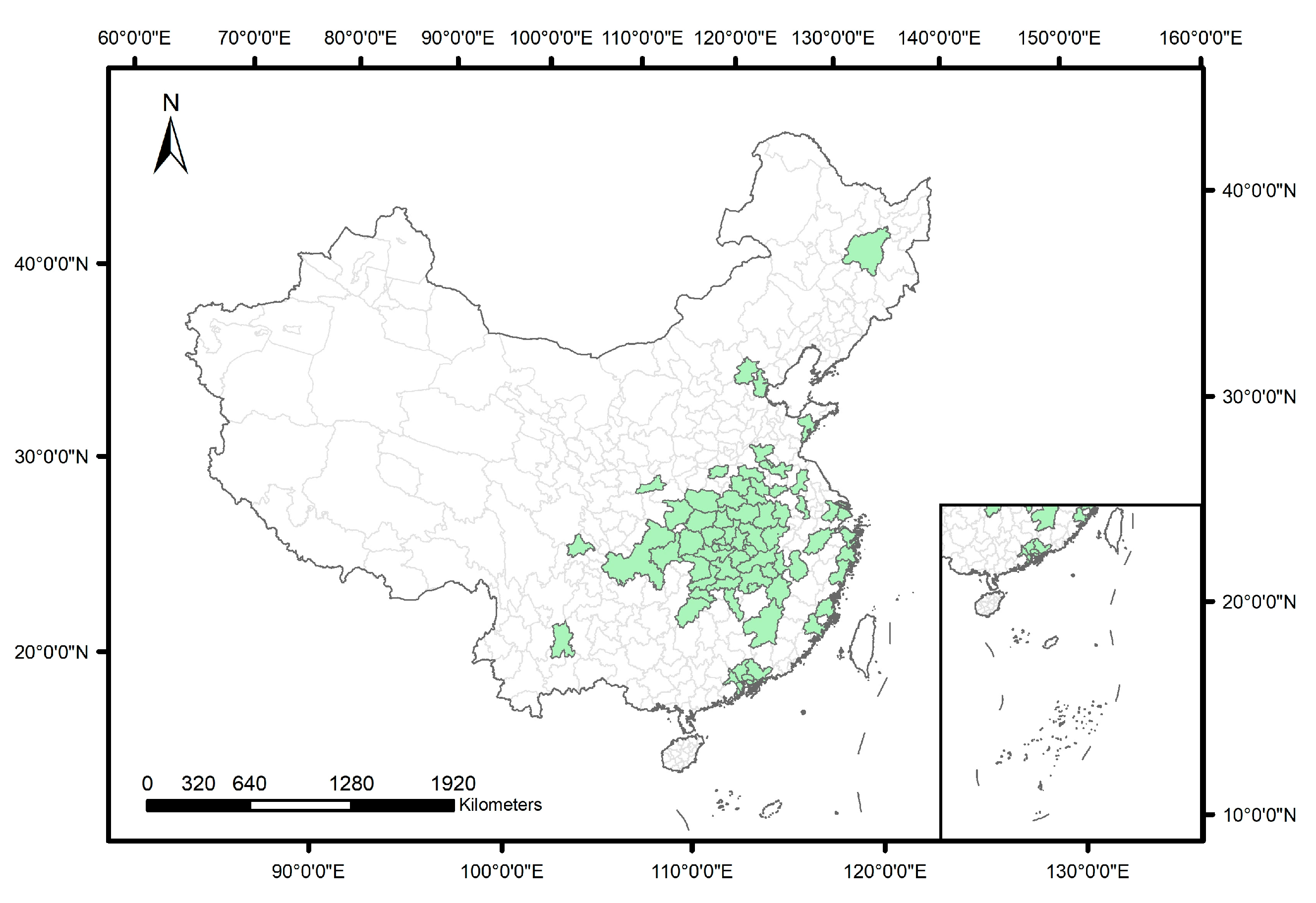
2.1. Study Area

In this research, 61 typical cities in Mainland China with a total number of confirmed cases larger than 60 until 12 March 2020 (the day when the first wave of COVID-19 pandemic in Chinese mainland was under control) were selected as the study area, as they experienced relatively more severe pandemic shock. The research focused on a six-week study period from 30 January 2020 (the week following the announcement of Wuhan lockdown) to 12 March 2020. The study area is shown in Figure 1.

2.2. Methodology

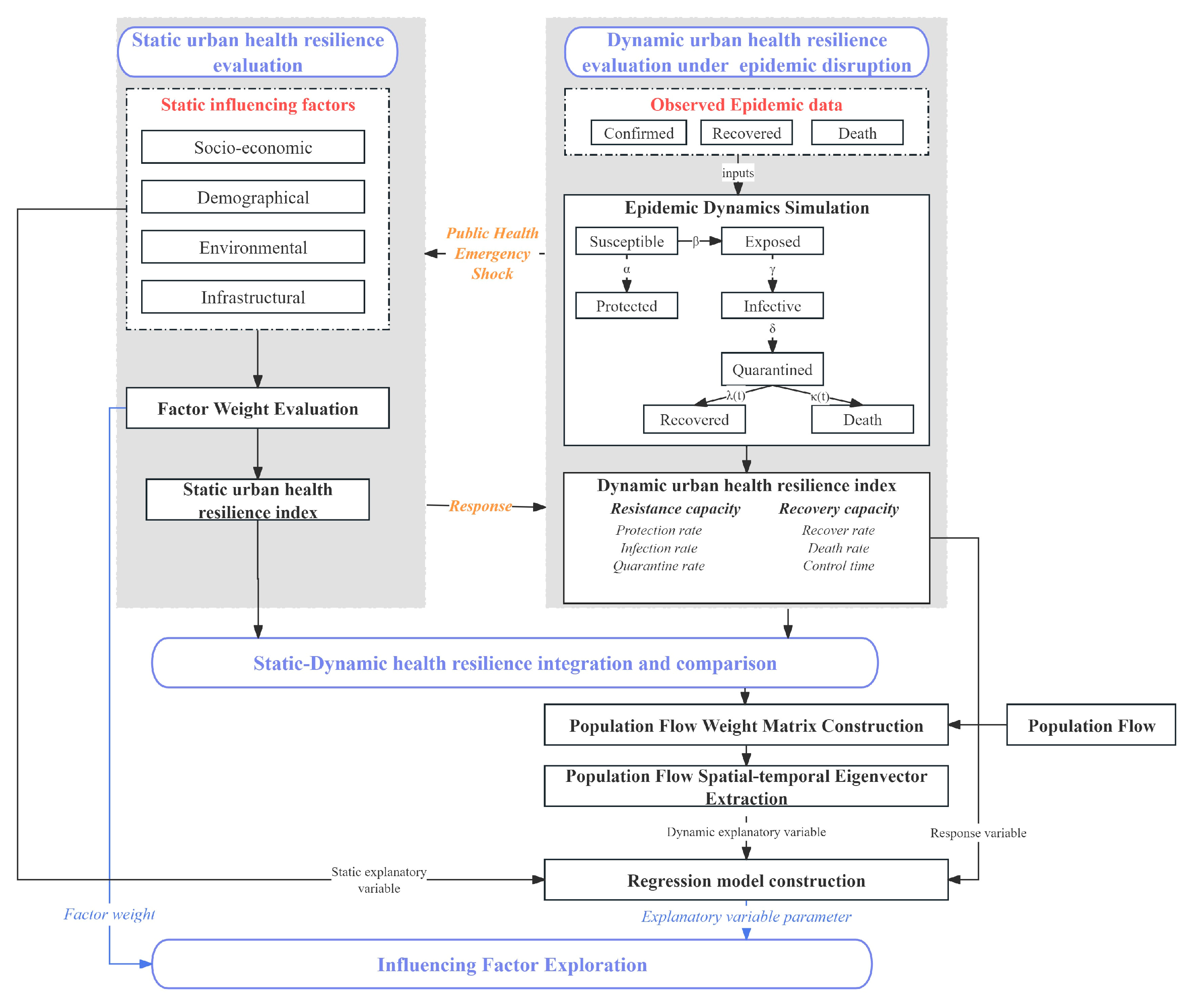
2.2.1. Analytical Framework Construction

In this study, a static–dynamic analytical framework for urban health resilience evaluation and influencing factor exploration was proposed (Figure 2).

Firstly, based on existing resilience theory frameworks [33,36,37,38], relatively static factors were selected from four fundamental but critical aspects (social–economical, demographical, environmental and infrastructural ones [39,40,41,42]) to evaluate the static urban health resilience index (SUHRI) in normal conditions, as shown in

Table 1. Influencing factors and data resources.

	Type	Criterion	Indicator	Abbreviation	Data Sources
Influencing factors	Static	Infrastructure	POI density	POI	Baidu map service platform (https://lbsyun.baidu.com/), accessed on 20 June 2023.
			Hospital capacity (sick bed and doctor number)	HOS	The Statistical year book of 2019 (https://navi.cnki.net/knavi/), accessed on 9 April 2025.
			Mobile phone rate	PHONE
			Internet Rate	INTER
		Socioeconomic	Income level	INCOME
			Medical insurance	MISU
			Elderly care insurance	EISU
			Education level	ILLE
		Demographic	Population density	POP
			Aging ratio	A65
			Young age ratio	U15
		Environmental	Green ratio	GR
			Annual average Air quality	PM25
	Dynamic	Human Mobility	Initial inflow from Wuhan before lockdown	Wh_qx	Baidu Qianxi Platform (https://qianxi.baidu.com/), accessed on 27 July 2021.
			Population migration flow among cities	/

. The social–economical dimension reflects resource allocation capabilities, demographic characteristics reflects population vulnerability [4,5,6], environmental factors might be related to mediate exposure risks [43], while infrastructural construction may influence material and information supply, as well as the intensity of potential human activity and interaction within a city [44,45,46,47,48]. The SUHRI was calculated after evaluating the weights of the selected factors. The SUHRI could reflect the theoretical resource preparedness. Urban systems with higher SUHRI are expected to have better resist and recovery capacity against public health emergencies.

Secondly, according to the epidemic response metrics validated by the WHO [49] and existing studies on resilience to pandemics [33,50], sub-indices from both resistance and recovery capacity aspects were selected to represent the dynamic urban health resilience index (DUHRI). Sub-indices from the resistance aspect include protection rate, infection rate, and quarantine rate, which reflect the strength to mitigate pandemic transmission [51,52,53], while sub-indices from the recovery aspect include recovery rate, death rate, and epidemic control time, which reflect the ability to recover from a crisis and achieve stabilization [54,55,56]. The DUHRI sub-indices were estimated using an epidemic dynamic simulation method. Observed time-series empirical epidemic data (including daily confirmed (C), recovered (R) and death cases (D) reported by The National Health Commission) were collected and served as foundational inputs and reference points for epidemic dynamic simulation. Through model parameter estimation, sub-indices in the DUHRI (protection rate, infection rate, recovery rate, etc.) were derived, reflecting the actual response under the COVID-19 shock. Cities with better resistance capacity had a higher protection rate, higher quarantine rate, and lower infection rate, while cities with better recovery capacity had a higher recovery rate, lower death rate, and shorter control time.

SUHRI reflects the theoretical preparedness level against pandemics, while DUHRI reflects actual dynamic performance during pandemic crises. The health emergency exerts pressure on the basic urban system, and the factors in SUHRI help to respond to the pandemic, feeding back into the presence of DUHRI. For example, a better economic status in SUHRI might lead to more comprehensive protective measures, which theoretically feed back into a higher protection rate in DURHI. However, DURHI might not only be influenced by factors in SUHRI but also be influenced by other instant dynamical factors, such as population flow, policy response, etc.

Therefore, the third step was to further explore the relationship between SUHRI and DUHRI. The following measures were taken: (a) a scatter plot between SUHRI and DUHRI was applied to conduct a generative comparison; (b) the static–dynamic integration score and static–dynamic difference score were calculated to analyze the integration and differences between SUHRI and DUHRI. SUHRI was ranked into five classes (with score from 1 to 5) using a quantile method to yield SUHRI rank score. The sub-indices of DUHRI were also ranked into five classes, and the average rank scores of the sub-indices were calculated to yield the final DUHRI rank score. The static–dynamic integration score was calculated by averaging the SUHRI rank score and DUHRI rank score, while the static–dynamic difference score was calculated by subtracting the SUHRI rank score from the DUHRI rank score. The larger the static–dynamic integration score, the better a city performs in both static resilience and in dynamic resilience, while the larger the static–dynamic difference score, the stronger a city’s dynamic resilience level outperforms its static resilience level in the context of pandemic.

Fourthly, as the DUHRI that reflects the actual response in the context of pandemics could not only be influenced by relatively static factors but also by other dynamic factors such as population flow, a FLOW-ESTF regression method was adopted. It evaluates the mobility connection among cities, depositing the matrix into spatial–temporal eigenvectors that represent the characteristics of population flow autocorrelation. After adding selected population flow eigenvectors into the modeling, the final FLOW-ESTF model could improve model accuracy and be better prepared for DUHRI influencing factor exploration.

The final step was to explore how the selected factors influenced SUHRI and DUHRI based on the above modeling results. The AHP–entropy weight evaluation results reflect the static factors’ contribution to SUHRI; the larger the weights, the greater the contribution of the corresponding factor to SUHRI. The FLOW-ESTF regression model coefficients reflect both how static factors and population flow spillover effects impact DUHRI.

The results of SUHRI and DUHRI, along with their corresponding key influencing factors, were compared and discussed. The data sources for the selected influencing factors are shown in Table 1. The static–dynamic analytical framework above could help not only to analyze basic urban health resilience under normal conditions but also to evaluate urban health resilience under external epidemic shocks.

2.2.2. Static Urban Health Resilience Index Calculation

One important issue in calculating SUHRI is determining indicator weights [31]. The widely used AHP method is based on expert experience but tends to be subjective, while entropy weight method based on observed data is objective but relies on sample size and data quality. Therefore, in this study, the AHP–entropy method, which considers both subjective and objective perspectives [57], was taken to evaluate SUHRI factor weights.

Static indicators were firstly divided into positive and negative influence indicators. The higher a positive indicator value, the higher the health resilience indices in the context of pandemic, and vice versa. Positive indicators include HOS, PHONE, INTER, INCOME, MISU, EISU and GR, while negative indicators include POI, ILLE, POP, A65, U15 and PM25. Positive and negative indicators were standardized, as shown in Equations (1) and (2), respectively.

$${\mathrm{x}}_{\mathrm{i}}={\displaystyle \frac{{\mathrm{x}}_{\mathrm{i}}-{\mathrm{x}}_{\mathrm{m}\mathrm{i}\mathrm{n}}}{{{\mathrm{x}}_{\mathrm{m}\mathrm{a}\mathrm{x}}-\mathrm{x}}_{\mathrm{m}\mathrm{i}\mathrm{n}}}}$$

(1)

$${\mathrm{x}}_{\mathrm{i}}={\displaystyle \frac{{\mathrm{x}}_{\mathrm{m}\mathrm{a}\mathrm{x}}{-\mathrm{x}}_{\mathrm{i}}}{{{\mathrm{x}}_{\mathrm{m}\mathrm{a}\mathrm{x}}-\mathrm{x}}_{\mathrm{m}\mathrm{i}\mathrm{n}}}}$$

(2)

Then, pairwise comparison matrices were made to represent relative importance between indicators, as shown in Equation (3):

$$A=\left(\begin{array}{cccc}1& a_{12}& \cdots & a_{1k}\\ a_{21}& 1& ⋮& a_{2k}\\ ⋮& ⋮& \ddots & ⋮\\ a_{k1}& a_{k2}& \cdots & a_{kk}\end{array}\right),$$

(3)

where $A$ is the symmetric pairwise comparison matrix; $a_{ij}$ represents the importance level when comparing indicator i to indicator j, ${\mathrm{a}}_{\mathrm{j}\mathrm{i}}$ = 1/${\mathrm{a}}_{\mathrm{i}\mathrm{j}}$; the larger ${\mathrm{a}}_{\mathrm{i}\mathrm{j}},$ the more important indicator i is compared to indicator j in the context of urban health resilience; $k$ is the number of indicators. A total of 10 experts were invited to give the importance comparison score. Then, “ahpsurvey” package in R-Studio (version R 4.3.2) was used to test consistency of the comparison matrix and finally yield the AHP weight vector ${\mathrm{W}}_{\mathrm{A}\mathrm{H}\mathrm{P}}=({\mathrm{w}}_{\mathrm{a}1},{\mathrm{w}}_{\mathrm{a}2},\dots ,{\mathrm{w}}_{\mathrm{a}\mathrm{k}})$.

Then, use the entropy method to obtain objective indicator weights. The calculations are as follows:

Step 1: For each indicator i, calculate the entropy ${\mathrm{e}}_{\mathrm{i}}$:

$${\mathrm{e}}_{\mathrm{i}}={\displaystyle \frac{-\sum _{\mathrm{j}=1}^{\mathrm{n}}{\mathrm{p}}_{\mathrm{i}\mathrm{j}}\mathrm{l}\mathrm{n}{\mathrm{p}}_{\mathrm{i}\mathrm{j}}}{\mathrm{l}\mathrm{n}\mathrm{n}}}(\mathrm{i}=1,2,\dots ,\mathrm{k};\mathrm{j}=1,2,\dots ,\mathrm{n})$$

(4)

$${\mathrm{p}}_{\mathrm{i}\mathrm{j}}={\displaystyle \frac{{\mathrm{x}}_{\mathrm{i}\mathrm{j}}}{\sum _{\mathrm{j}=1}^{\mathrm{n}}{\mathrm{x}}_{\mathrm{i}\mathrm{j}}}}(\mathrm{i}=1,2,\dots ,\mathrm{k};\mathrm{j}=1,2,\dots ,\mathrm{n})$$

(5)

where $\mathrm{k}$ is the number of indicators, n is the number of study units, ${\mathrm{x}}_{\mathrm{i}\mathrm{j}}$ is the standardized i th indicator value for unit j.

Step 2: Calculate the entropy weight ${\mathrm{w}}_{\mathrm{e}\mathrm{i}}$ for i th indicator, as shown in Equation (6):

$${\mathrm{w}}_{\mathrm{e}\mathrm{i}}={\displaystyle \frac{1-{\mathrm{e}}_{\mathrm{i}}}{\sum _{\mathrm{i}=1}^{\mathrm{k}}(1-{\mathrm{e}}_{\mathrm{i}})}}(\mathrm{i}=1,2,\dots ,\mathrm{k})$$

(6)

The final AHP–entropy weight ${\mathrm{w}}_{\mathrm{i}}$ was calculated by the average AHP weight and the entropy weight:

$${\mathrm{w}}_{\mathrm{i}}=0.5\times ({\mathrm{w}}_{\mathrm{a}\mathrm{i}}+{\mathrm{w}}_{\mathrm{e}\mathrm{i}})$$

(7)

With the final AHP–entropy weight, the SUHRI was calculated using Equation (8):

$$\mathrm{S}\mathrm{U}\mathrm{H}\mathrm{R}\mathrm{I}={\sum }_{\mathrm{i}=1}^{\mathrm{k}}{\mathrm{w}}_{\mathrm{i}}\times {\mathrm{x}}_{\mathrm{i}}$$

(8)

2.2.3. Dynamic Urban Health Resilience Index Calculation

The dynamic urban health resilience index (DUHRI) consists of sub-indices, including resistance capacity (protection rate, infection rate and quarantine rate) and recovery capacity (recovery rate, death rate and epidemic control time). The descriptions of corresponding sub-indices are shown in

Table 2. Description for dynamic urban health resilience indices.

DUHRI	Sub-Index	Description
Resistance capacity	$\mathrm{Protection} \mathrm{rate} \left(\mathsf{\alpha }\right)$	Population that protected from infected cases, either by vaccination or by strictly quarantined from infected cases.
	$\mathrm{Infection} \mathrm{rate} \left(\mathsf{\beta }\right)$	The possibility of susceptible individuals being infected after being exposed to infected individuals.
	$\mathrm{Quarantine} \mathrm{rate} \left(\mathsf{\delta }\right)$	The speed of infected cases entered quarantine.
Recovery capacity	$\mathrm{Recovery} \mathrm{rate} \mathsf{\lambda }\left(\mathrm{t}\right)$	The ratio of daily recovered cases versus existing active (quarantined) cases.
	$\mathrm{Death} \mathrm{rate}\mathsf{\kappa }\left(\mathrm{t}\right)$	The ratio of daily death cases versus existing active (quarantined) cases.
	Control time (T2)	The number of day that the existing active cases decline from peak to minimum and kept not rising for more than 7 days at the first wave of pandemic.

. It should be noted that, typically, the protection rate represents the proportion of the population protected from infection, either through vaccination or strict quarantine measures. However, since the vaccine had not been developed during the early stages of the COVID-19 pandemic, the protection rate reflects the effectiveness of protection measures such as quarantine from infected cases.

The Generalized Susceptible–Exposed–Infectious–Recovered model (SEIQRDP), an extension of the SEIR model incorporating considerations of control measures, which could effectively simulate the epidemic dynamics [58,59,60], was applied to quantitatively evaluate sub-indices in DUHRI against public health emergency.

The total population within a study unit was divided into seven categories: susceptible, exposed, infected, quarantined, recovered, dead and protected. The transitions between these categories are shown in Figure 2. The corresponding differential equation is shown in Equation (9):

$$\left\{\begin{array}{c}{\displaystyle \frac{\mathrm{d}{\mathrm{S}}_{\mathrm{i}}(\mathrm{t})}{\mathrm{d}\mathrm{t}}}=-{\mathsf{\beta }}_{\mathrm{i}}{\displaystyle \frac{{\mathrm{S}}_{\mathrm{i}}(\mathrm{t}){\mathrm{I}}_{\mathrm{i}}(\mathrm{t})}{{\mathrm{N}}_{\mathrm{i}}}}-{\mathsf{\alpha }}_{\mathrm{i}}{\mathrm{S}}_{\mathrm{i}}(t)\\ {\displaystyle \frac{\mathrm{d}{\mathrm{E}}_{\mathrm{i}}(\mathrm{t})}{\mathrm{d}\mathrm{t}}}={\mathsf{\beta }}_{\mathrm{i}}{\displaystyle \frac{{\mathrm{S}}_{\mathrm{i}}(\mathrm{t}){\mathrm{I}}_{\mathrm{i}}(\mathrm{t})}{{\mathrm{N}}_{\mathrm{i}}}}-{{\mathsf{\gamma }}_{\mathrm{i}}\mathrm{E}}_{\mathrm{i}}(t) \\ {\displaystyle \frac{\mathrm{d}{\mathrm{I}}_{\mathrm{i}}(\mathrm{t})}{\mathrm{d}\mathrm{t}}}={\mathsf{\gamma }}_{\mathrm{i}}{\mathrm{E}}_{\mathrm{i}}(t)-{\mathsf{\delta }}_{\mathrm{i}}{\mathrm{I}}_{\mathrm{i}}(t) \\ {\displaystyle \frac{\mathrm{d}{\mathrm{Q}}_{\mathrm{i}}(\mathrm{t})}{\mathrm{d}\mathrm{t}}}={\mathsf{\delta }}_{\mathrm{i}}{\mathrm{I}}_{\mathrm{i}}(t)-{\mathsf{\lambda }}_{\mathrm{i}}(t){\mathrm{Q}}_{\mathrm{i}}(t)-{\mathsf{\kappa }}_{\mathrm{i}}(t){\mathrm{Q}}_{\mathrm{i}}(t)\\ {\displaystyle \frac{\mathrm{d}{\mathrm{R}}_{\mathrm{i}}(\mathrm{t})}{\mathrm{d}\mathrm{t}}}={\mathsf{\lambda }}_{\mathrm{i}}(t){\mathrm{I}}_{\mathrm{i}}(t)\\ {\displaystyle \frac{\mathrm{d}{\mathrm{D}}_{\mathrm{i}}(\mathrm{t})}{\mathrm{d}\mathrm{t}}}={\mathsf{\kappa }}_{\mathrm{i}}(t){\mathrm{I}}_{\mathrm{i}}(t)\\ {\displaystyle \frac{\mathrm{d}{\mathrm{P}}_{\mathrm{i}}(\mathrm{t})}{\mathrm{d}\mathrm{t}}}={\mathsf{\alpha }}_{\mathrm{i}}{\mathrm{S}}_{\mathrm{i}}(t) \end{array}\right.$$

(9)

where ${\mathrm{S}}_{\mathrm{i}}\left(\mathrm{t}\right)$, ${\mathrm{E}}_{\mathrm{i}}\left(\mathrm{t}\right)$, ${\mathrm{I}}_{\mathrm{i}}\left(\mathrm{t}\right)$, ${\mathrm{Q}}_{\mathrm{i}}\left(\mathrm{t}\right)$, ${\mathrm{R}}_{\mathrm{i}}\left(\mathrm{t}\right)$, ${\mathrm{D}}_{\mathrm{i}}\left(\mathrm{t}\right)$, ${\mathrm{P}}_{\mathrm{i}}\left(\mathrm{t}\right)$ are the number of susceptible, exposed (infected but in the incubation period), infective (but not yet quarantined), recovered, dead and quarantined cases in unit i at time t, respectively. Note that ${\mathrm{S}}_{\mathrm{i}}\left(\mathrm{t}\right)$ + ${\mathrm{P}}_{\mathrm{i}}\left(\mathrm{t}\right)$ + ${\mathrm{E}}_{\mathrm{i}}\left(\mathrm{t}\right)$ + ${\mathrm{I}}_{\mathrm{i}}\left(\mathrm{t}\right)$ + ${\mathrm{Q}}_{\mathrm{i}}\left(\mathrm{t}\right)$ + ${\mathrm{R}}_{\mathrm{i}}\left(\mathrm{t}\right)$ + ${\mathrm{P}}_{\mathrm{i}}\left(\mathrm{t}\right)$ = ${\mathrm{N}}_{\mathrm{i}}$, ${\mathrm{N}}_{\mathrm{i}}$ is the total population in study unit i; ${\mathsf{\alpha }}_{\mathrm{i}}$, ${\mathsf{\beta }}_{\mathrm{i}}$, ${\mathsf{\gamma }}_{\mathrm{i}}$, ${\mathsf{\delta }}_{\mathrm{i}}$ are the protection rate, infection rate, inverse average latent time, inverse rate of infected people entering quarantine in study unit i; ${\mathsf{\lambda }}_{\mathrm{i}}\left(\mathrm{t}\right)$ and ${\mathsf{\kappa }}_{\mathrm{i}}\left(\mathrm{t}\right)$ are the time-dependent recovery rate and mortality rate, respectively.

For each study unit, the time series of observed COVID-19 pandemic data was collected. The epidemic data from the initial day of the study period served as foundational inputs for the SEIQRDP model, and initial parameter guesses were drawn from the empirical epidemiology studies. The ordinary differential equations in Equation (9) were solved using the Euler method. The “lsqcurvefit” function in MATLAB (version 9.14) was applied for nonlinear parameter optimization, with the initial parameter guesses being iteratively refined to minimize the error between the simulation outputs and observed epidemic values [61]. By effectively capturing the epidemic dynamics, the optimized parameters could be taken as public health emergency resistance and recovery capacity sub-indices [60]. The higher the protection rate and the quarantine rate, or the lower the infection rate, the better the resistance capacity, while the higher the recovery rate, or the lower the death rate and control time, the better the recovery capacity.

2.2.4. Population Flow-Based Spatial–Temporal Eigenvector Filtering Model Construction

The population flow-based spatial–temporal eigenvector filtering method (FLOW-ESTF) [35] was adopted to extract the influence of population flow autocorrelation in modeling. The indices in DUHRI were taken as dependent variables, while static influencing factors and population flow-related variables were taken as independent variables. As time-varying indices in DUHRI fluctuate across days, to better evaluate the overall trend, the dynamic time-varying indices were averaged over weeks.

The construction of the FLOW-ESTF model includes the following steps:

Step 1: Build dynamic population flow weight matrix ${\mathrm{F}}_{\mathrm{t}}$ to capture the population flow autocorrelation among cities at week t, as shown in Equation (10).

$$F_t=\left(\begin{array}{cccc}0& f_{\mathrm{1,2},t}& \cdots & f_{1,n,t}\\ f_{\mathrm{2,1},t}& 0& ⋮& f_{2,n,t}\\ ⋮& ⋮& 0& ⋮\\ f_{n,1,t}& f_{n,2,t}& \cdots & 0\end{array}\right),$$

(10)

where $f_{i,j,t}$ is the weekly population inflow intensity data from city i to city j at week t. The larger $f_{i,j,t}$, the stronger population flow autocorrelation between city i and city j at week t.

Step 2: Establish temporal weight matrix T to represent temporal autocorrelation. The calculation of elements ${\mathrm{T}}_{\mathrm{i}\mathrm{j}}$ in matrix T is shown in Equation (11),

$$\begin{array}{c}\left\{\begin{array}{c}{\mathrm{T}}_{\mathrm{i}\mathrm{j}}={\displaystyle \frac{1}{\left|\mathrm{j}-\mathrm{i}\right|}} \left(\mathrm{i}\ne \mathrm{j} \mathrm{and} \left|\mathrm{j}-\mathrm{i}\right|<threshold\right)\\ {\mathrm{T}}_{\mathrm{i}\mathrm{j}}=0 \left(\mathrm{i}=\mathrm{j} \mathrm{or} \left|\mathrm{j}-\mathrm{i}\right|\ge threshold\right)\end{array}\right.\end{array}$$

(11)

where i and j are the time indices (week IDs) throughout the study period; threshold is the temporal autocorrelation threshold. Considering the average incubation period of 1 week, the previous and next weeks were determined as correlated, while others were not, that is, threshold = 2.

Step 3: Then, calculate the final spatial–temporal weight matrix $F_{t}T$ to capture the spatial–temporal autocorrelation according to the spatial–temporal dependence expansion method [35,62], as shown in Equation (12):

$$F_{t}T=I_T\otimes F_t+T\otimes I_S$$

(12)

where $I_T$ is the time dimension identity matrix, $I_S$ is the spatial dimention identity matrix, and $\otimes$ is the Kronecker product.

Step 4: The $F_{t}T$ matrix is centralized into $F_{t}CT$ and decomposed into eigenvectors, as shown in Equation (13):

$$F_{t}CT=\left(I-{\displaystyle \frac{{11}^T}{nt}}\right)F_{t}T\left(I-{\displaystyle \frac{{11}^T}{nt}}\right)={{EV}_{FCT}\wedge {EV}_{FCT}}^T$$

(13)

where n is the number of cities, t is the time dimension, and I is the identity matrix. ${EV}_{FCT}$ = $({\mathrm{E}\mathrm{V}}_{\mathrm{F}1},{\mathrm{E}\mathrm{V}}_{\mathrm{F}2},\dots ,{\mathrm{E}\mathrm{V}}_{\mathrm{F}\mathrm{n}\mathrm{t}})$ represents the collection of population flow spatial–temporal autocorrelation eigenvectors sorted by corresponding eigenvalues from the largest to the smallest, and $\wedge$ is a diagonal matrix of the eigenvector-related eigenvalues (${\mathsf{\lambda }}_{\mathrm{F}1}$, ${\mathsf{\lambda }}_{\mathrm{F}2}$, ${\mathsf{\lambda }}_{\mathrm{F}3}$,…, ${\mathsf{\lambda }}_{\mathrm{F}\mathrm{n}\mathrm{t}}$).

Step 5: Stepwise method was used for eigenvector selection and to address multicollinearity issues in variables [63], ensuring that the variance inflation factor value (VIF) between selected influencing factors was less than 10. Then, the final selected eigenvectors, representing external disturbance caused by population flow interaction, were added into DUHRI influencing factor modeling. The construction of DUHRI influencing factor model is shown in Equation (14):

$$\mathrm{R}(\mathrm{t})={\displaystyle \frac{1}{\mathrm{I}\mathrm{’}\left(\mathrm{t}\right)}}={\mathsf{\beta }}_0+\sum _{\mathrm{p}=1}^{\mathrm{p}=\mathrm{p}1}{\mathsf{\beta }}_{\mathrm{p}}{\mathrm{X}}_{\mathrm{p},\mathrm{t}}+\sum _{\mathrm{m}=1}^{\mathrm{m}=\mathrm{p}2}{\mathsf{\beta }}_{\mathrm{m}}{\mathrm{E}\mathrm{V}}_{\mathrm{F}\mathrm{n},\mathrm{t}}+\mathsf{\epsilon }$$

(14)

where $\mathrm{R}\left(\mathrm{t}\right)$ is the sub-index of DUHRI shown in Table 2. For time-varying sub-indices $\mathsf{\lambda }\left(\mathrm{t}\right)$ and $\mathsf{\kappa }\left(\mathrm{t}\right)$, t denotes the week index throughout study period; for time-constant sub-indices $\mathsf{\alpha },\mathsf{\beta },\mathsf{\delta },\mathrm{T}2$, the time index t and the time weight matrix T are downscaled to 1; $\mathrm{p}1$ is the number of potential influencing factors; ${\mathrm{X}}_{\mathrm{p},\mathrm{t}}$ is a $\mathrm{n}\times 1$ vector of the p-th influencing factor at time t; $\mathrm{p}2$ is the number of selected population flow eigenvectors, which varies by DUHRI; ${\mathrm{E}\mathrm{V}}_{\mathrm{F}\mathrm{n},\mathrm{t}}$ is the n-th population flow spatial–temporal eigenvector specimen at time t; ${\mathsf{\beta }}_0,{\mathsf{\beta }}_{\mathrm{k}},{\mathsf{\beta }}_{\mathrm{m}}$ are the simultaneously estimated regression coefficients; $\mathsf{\epsilon }$ is random error.

The performance of FLOW-ESTF method is compared with that of existing basic multiple linear regression (MLR), geographical weighted regression [64] (GWR) and Eigenvector Spatial Temporal Filtering (ESTF) [62] models. By filtering out the influence of population flow patterns, the final FLOW-ESTF model could improve model accuracy and be better prepared to explore how each potential influencing factor and population flow spillover effects impact dynamic urban health resilience, respectively.

2.2.5. Influencing Factor Exploration

The final influencing factor exploration is based on the above modeling results. The factor weight result ${\mathrm{w}}_{\mathrm{i}}$ evaluated using the AHP–entropy method in Section 2.2.2 was chosen to reflect the static factor contribution to SUHRI. The larger ${\mathrm{w}}_{\mathrm{i}}$, the greater the corresponding factor i contributes to SUHRI. The FLOW-ESTF regression model coefficients were chosen to reflect how both static factors and population flow impacted DUHRI. The larger the absolute value of regression coefficients, the greater the corresponding factor contribution to DUHRI.

3. Results

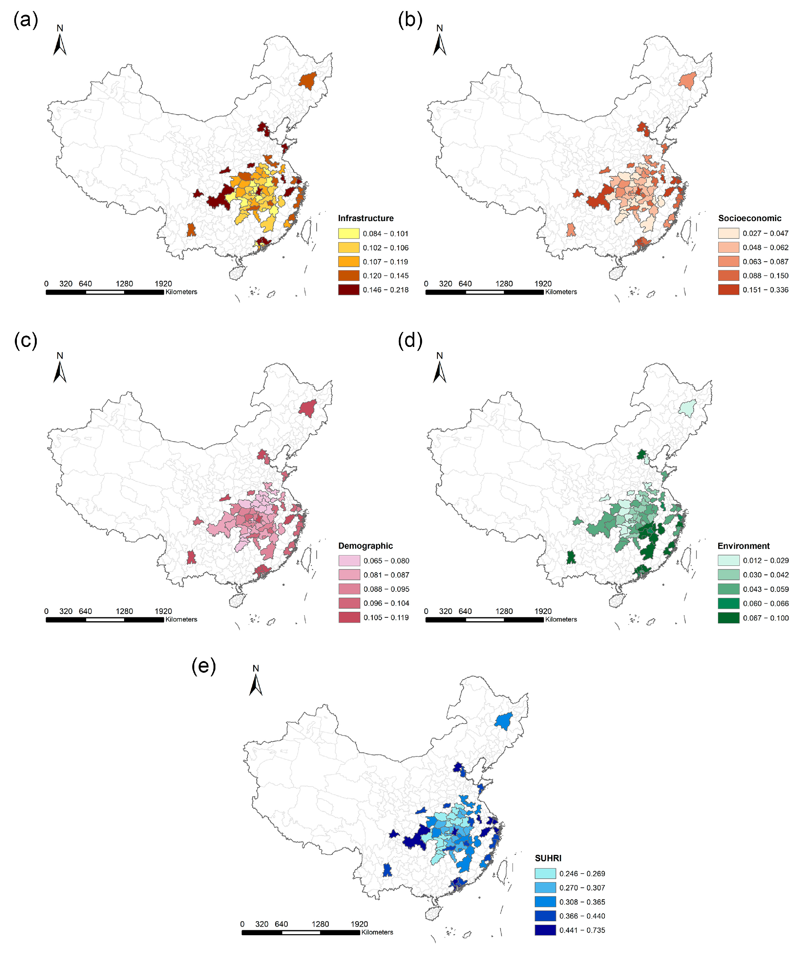
3.1. Static Urban Health Resilience Index Calculation Result

The static urban health resilience index (SUHRI) calculation result is shown in Figure 3. At the criterion level, in terms of infrastructure subsystems (Figure 3a), cities with higher scores are mainly distributed in municipalities, such as Chongqing, Beijing, Shanghai, and Tianjin, along with southern cities like Guangzhou, Shenzhen, and Hangzhou. Notably, Harbin, the northernmost city within this study’s scope, also exhibits a relatively high score. The spatial pattern of socioeconomical subsystem scores (Figure 3b) is generally consistent with those of infrastructure subsystems. However, central cities tend to have higher demographical subsystem scores (Figure 3c), while southwestern cities tend to have higher environmental subsystem scores (Figure 3d). The final comprehensive SUHRI result in Figure 3e shows that, generally, municipalities and provincial capitals tend to have better static urban health resilience, whereas central and other non-capital cities generally have lower static urban health resilience.

3.2. Dynamic Urban Health Resilience Index Calculation Result

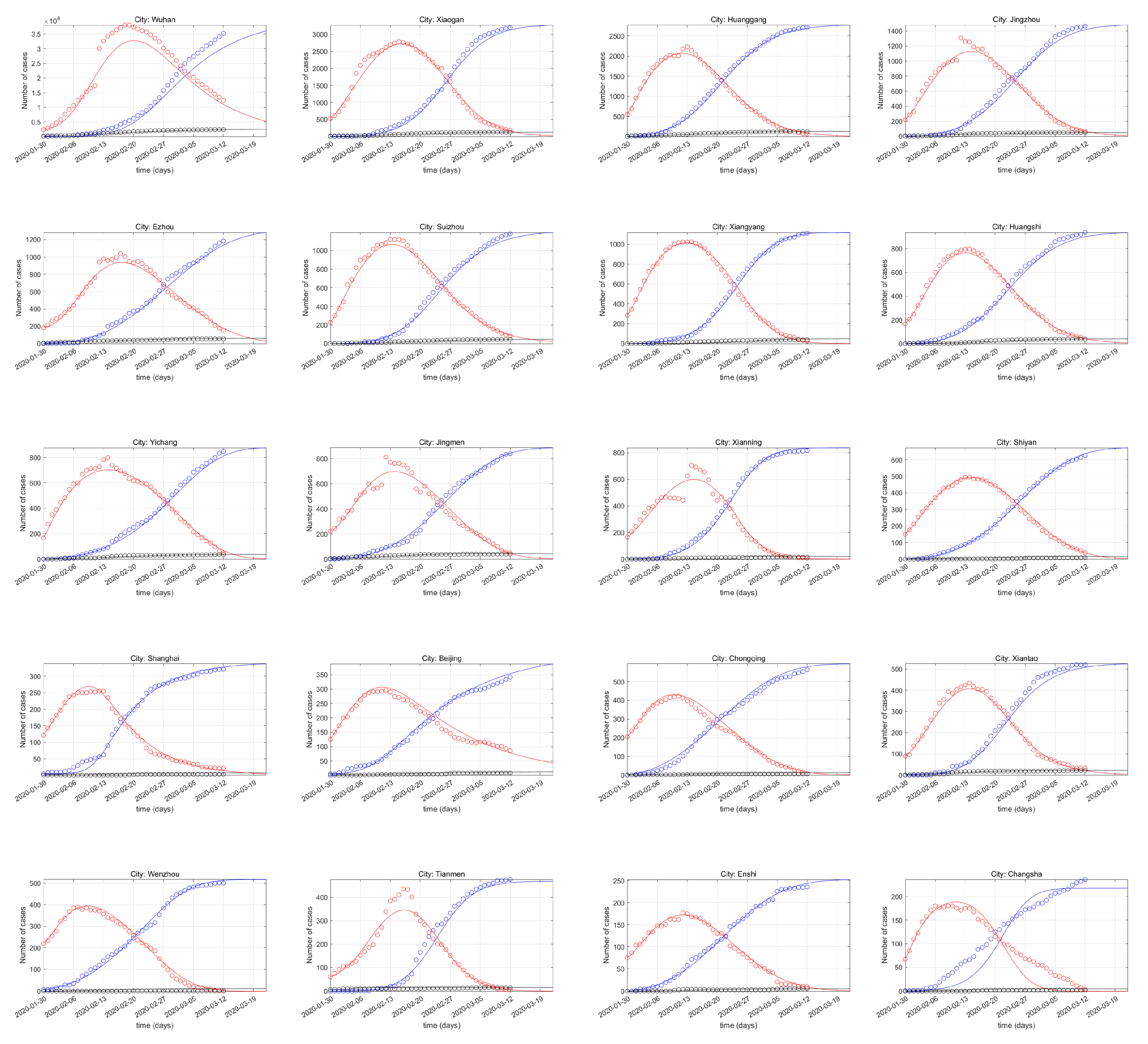
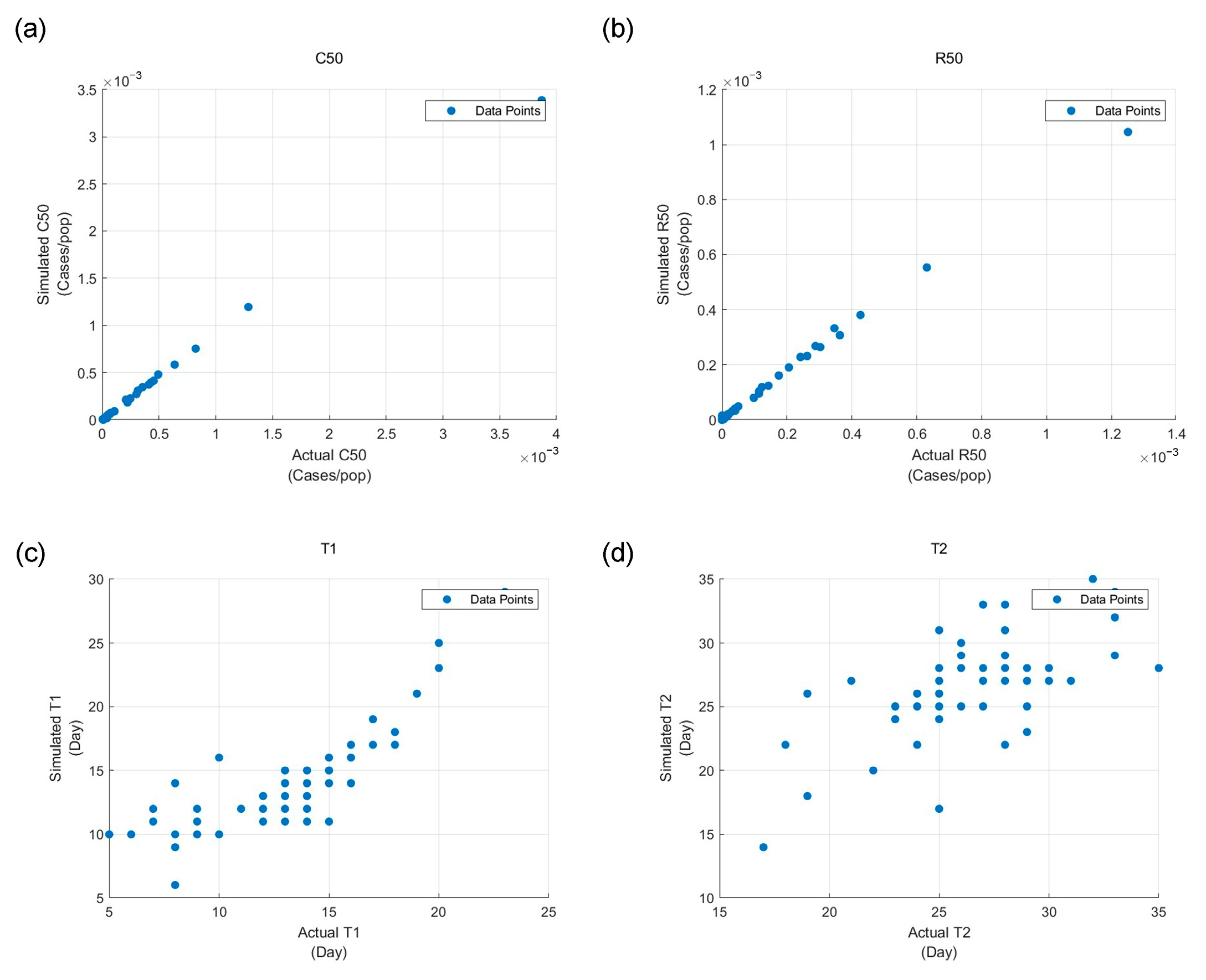
3.2.1. SEIQRDP Model Performance

Figure 4 shows the predicted Q, R, and D cases yielded by the SEIQRDP model (red, blue and black curve lines) and the corresponding reported quarantined, recovered and death cases (red, blue and black circles) in the top-20 cumulative confirmed cities in Mainland China. The results showed that curves between predicted cases and observed cases matched well. Furthermore, four epidemic key nodes, including the cumulative confirmed ratio 50 days after the announcement of the Wuhan City lockdown (C50), the cumulative recovered ratio 50 days after the announcement of the Wuhan City lockdown (R50), the time from beginning to reach the peak of active cases (T1), and the time to decline from the peak to the lowest point of the first wave (T2), were selected to reflect the epidemic dynamics. Figure 5a–d present scatter plots of the selected epidemic key nodes between observed and simulated ones, all of which showed high correlations, indicating that the SEIQRDP model could effectively capture the pandemic dynamics.

To evaluate the influence of parameter uncertainties on model robustness, sensitivity analysis was conducted using the Sobol method [65,66]. It quantifies the relative contribution of individual parameters to output variance through variance decomposition, achieved by systematically perturbing parameters within a variation range from estimated baseline parameter values (usually ±20%). First-order (S1) indices were calculated to identify dominant parameters and low-sensitivity variables. The larger the S1, and the more the corresponding parameter contributed to model outputs, the higher its sensitivity.

Considering the computational complexity and time-varying variance in time-varying parameters, the sensitivity analysis was conducted only on constant parameters $\mathsf{\alpha },\mathsf{\beta },\mathsf{\gamma },\mathsf{\delta }$. The boxplot for the S1 result is shown in Figure 6. The median values of S1 for $\mathsf{\alpha },\mathsf{\beta },\mathsf{\gamma },\mathsf{\delta }$ were 0.218, 0.312, 0.056 and 0.311, respectively. With higher S1 values, the infection rate and quarantine rate showed stronger sensitivity and were the dominant drivers of cumulative case predictions, reflecting their critical roles in governing transmission dynamics. The protection rate exhibited moderate sensitivity and was also an important driver for prediction. The interquartile range for both $\mathsf{\alpha }$ and $\mathsf{\delta }$ was large, which might be due to regional differences.

While $\mathsf{\gamma }$ had the lowest sensitivity and shortest range, it showed a weak impact in modeling. The inverse of the $\mathsf{\gamma }$ value represents the incubation period, which was mainly determined by the virus type. Previous studies have explained that the mean incubation period of COVID-19 at the early stage was about 5.1 days [67,68,69]. However, its narrow variability in return reflects model robustness. Therefore, $\mathsf{\gamma }$ was not taken as a sub-index of DUHRI.

The consistent sensitivity patterns without outliers demonstrated model simulation reliability, even under parameter variations. Therefore, the protection rate, infection rate and quarantine rate that strongly influence outcomes could be taken as sub-indices of DUHRI.

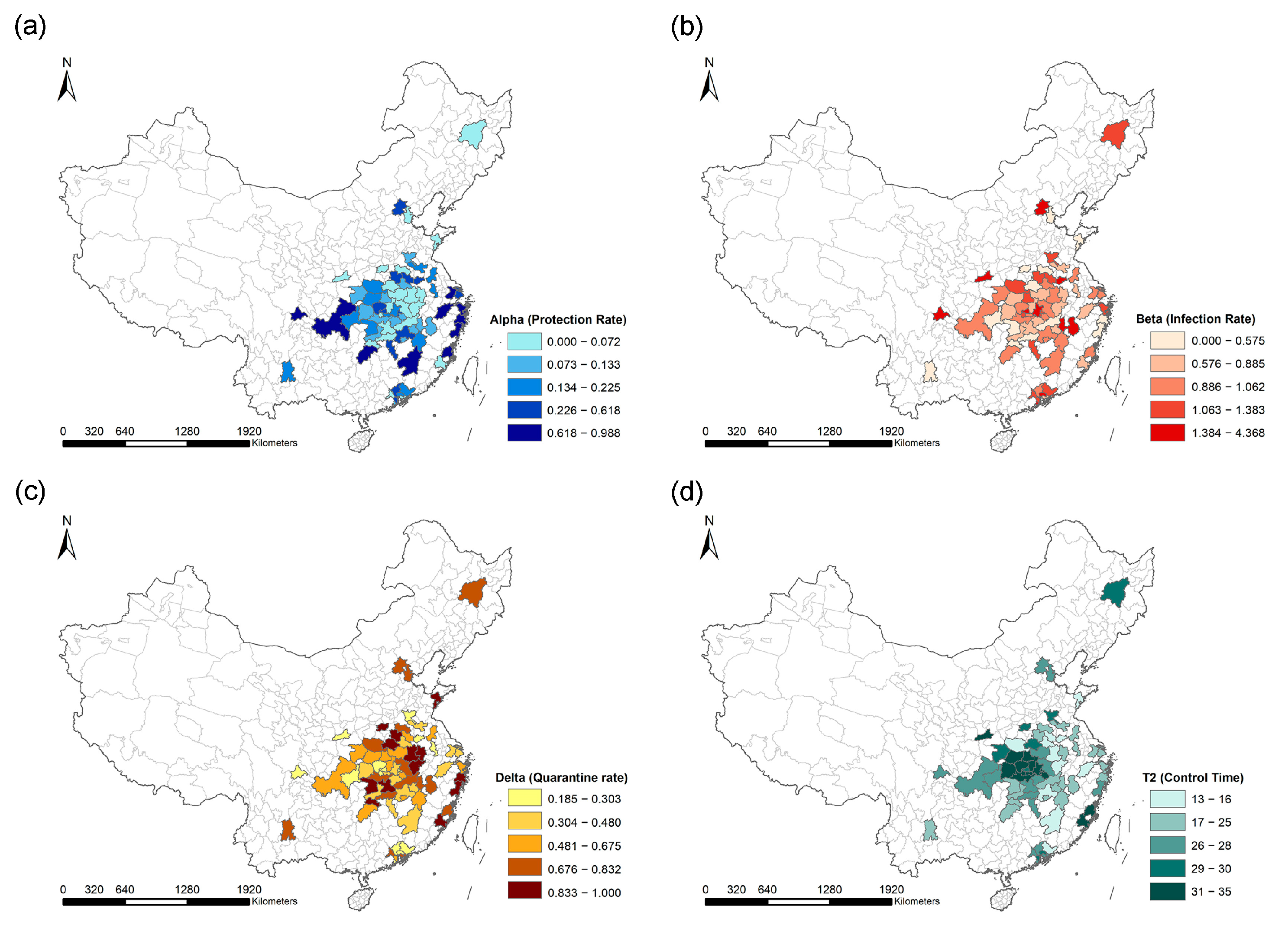
3.2.2. Public Health Emergency Resistance and Recovery Index Visualization

The protection rate $\mathsf{\alpha }$ is an important index for epidemic resistance in DUHRI, showing the intensity and effectiveness of protection measures. The higher the $\mathsf{\alpha }$ value, the better the preventive measures taken. As shown in Figure 7a, higher $\mathsf{\alpha }$ values were mostly distributed in southeastern coastal cities. A few central cities, including Zhengzhou, Nanyang, Changde, and Loudi, also exhibited relatively high values. Lower $\mathsf{\alpha }$ values were mainly distributed in cities around Wuhan. Particularly, $\mathsf{\alpha }$ values in Hefei, Lu’an, Xinyang, and Zhumadian were at the lowest level, even lower than those in most cities in Hubei provinces (including Wuhan).

The infection rate $\mathsf{\beta }$ is another index for epidemic health resistance in DUHRI, showing the proportion of susceptible individuals being infected through contact with infected individuals. The higher the $\mathsf{\beta }$ value, the easier individuals within a group tend to become infected. As shown in Figure 7b, higher $\mathsf{\beta }$ values were mostly distributed in central and northern provincial capitals, while lower $\mathsf{\beta }$ values were mostly distributed in southern coastal cities.

The quarantine rate $\mathsf{\delta }$ reflects the speed of infected individuals entering quarantine. The higher the quarantine rate, the better the epidemic health resistance capacity. As shown in Figure 7c, cities with larger $\mathsf{\delta }$ values and shorter average quarantine periods are primarily located in southern cities, such as Wenzhou, Taizhou and Quanzhou, and some central cities in Anhui, Henan and Hunan provinces. The $\mathsf{\delta }$ values in municipalities such as Beijing, Shanghai and Chongqing were not among the highest. The control time T2 reflects the recovery capacity of systemic response efficiency to control a pandemic from outbreak to sustained low risk. The shorter the T2, the better the recovery capacity. As shown in Figure 7d, cities with shorter T2 were mainly distributed in southeastern cities and a few central cities, while a longer T2 was mainly distributed in Hubei province around Wuhan.

Except for the above four constant parameters, the SEIQRDP model also yields two parameters that changed over time, λ(t) and $\mathsf{\kappa }(\mathrm{t}$), representing the recovery rate and death rate, respectively. As shown in Figure 8a,b, the recovery rates in all cities gradually increase over time. In terms of the death rate, except for Wuhan, the mortality rates in other cities all remain at a low level (<0.005). Wuhan’s death rate also rapidly declines, dropping below 0.005 by February 9th, and then remaining at the same level as that in other cities. The improvement in recovery rates and the reduction in mortality rates indicate an enhancement in the medical system’s recovery capacity.

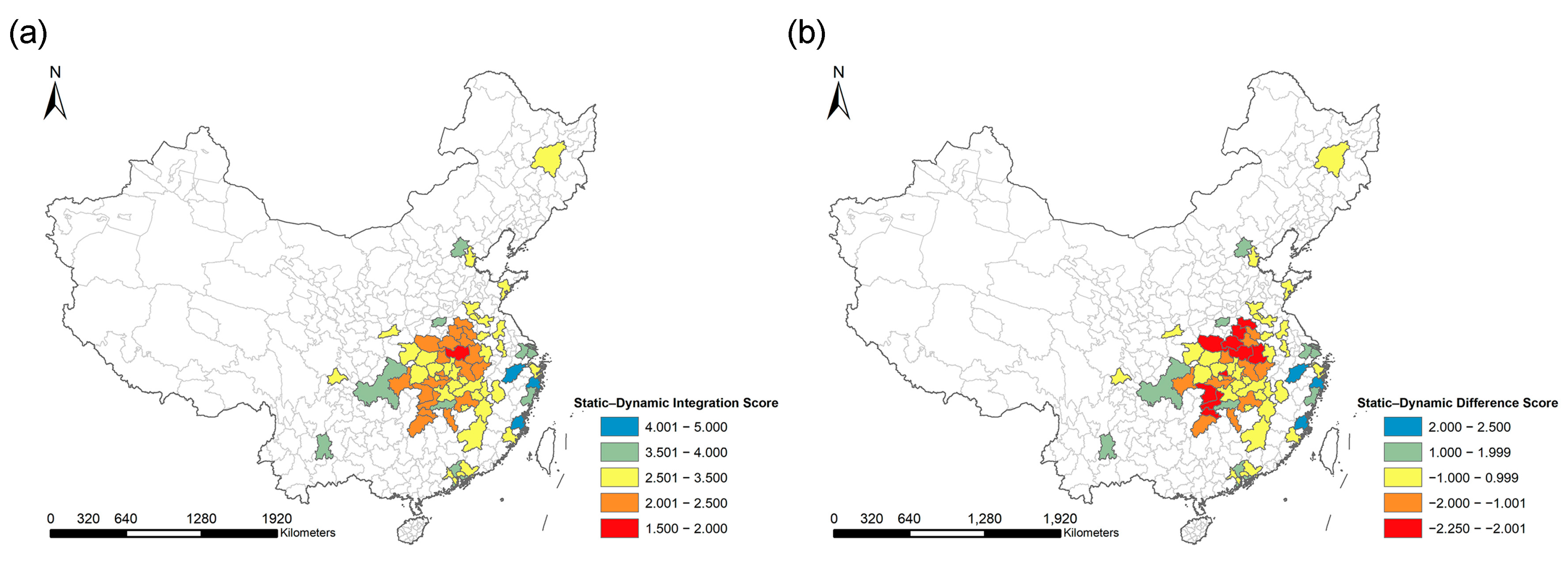
3.3. Static and Dynamic Urban Health Resilience Comparison and Integration

To further explore the relationship between SUHRI and DUHRI, a scatter plot is shown in Figure 9a–d, in which the X-axis represents the SUHRI score and the Y-axis represents sub-indices ($\mathsf{\alpha },\mathsf{\beta },\mathsf{\delta },\mathrm{T}2$) in DUHRI. In terms of resistance capacity, SUHRI showed a significant positive correlation with the protection rate $\mathsf{\alpha }$ (Figure 9a) and negative correlation with the infection rate $\mathsf{\beta }$ (Figure 9b), with coefficients of 0.51 and −0.34, respectively. The correlation between SUHRI and the quarantine rate $\mathsf{\delta }$ was also positive (Figure 9c) but relatively weaker (with a coefficient of 0.09). SUHRI showed a weakly negative correlation with epidemic control time T2 in Figure 9d, with a coefficient of −0.07. This might be due to a larger total number of infections in high SUHRI cities, making epidemic control also challenging. That is, generally, the higher the SUHRI, the higher the resistance capacity. However, the higher SUHRI was not significantly correlated with higher recovery capacity in DUHRI.

Then, to analyze SUHRI and DUHRI integration results and differences, the static–dynamic integration score and static–dynamic difference score were calculated.

The results of static–dynamic integration scores are shown in Figure 10a. The larger the static–dynamic integration score, the better a city performs both in static resilience and in dynamic resilience. Some southeastern cities including Hangzhou, Wenzhou and Taizhou had the highest rank of static–dynamic integration scores (above 4). Some regional hubs, such as Beijing, Shanghai, Shenzhen, and Guangzhou, ranked second in the static–dynamic integration scores. Some central cities in Hubei Province (including Wuhan) were at the mid rank of static–dynamic integration scores, while the lowest rank of static–dynamic integration scores was mostly distributed in central cities near Hubei province (such as Lu’an and Zhumadian).

Accordingly, the results of static–dynamic difference scores are shown in Figure 10b. The larger the difference scores, the stronger their dynamic resilience level outperforms the static resilience level in the context of a pandemic. The mid rank of static–dynamic difference scores (with absolute value less than 1) means that the performance of SUHRI and DUHRI is at the same level. Thus, 60.6% cities within the study area were at the mid rank of static–dynamic difference scores but also showed some typical differences. Some central cities in the southwest of Wuhan showed a higher rank of static–dynamic difference scores, despite their lower rank of static–dynamic integration scores. This indicates their limited performance on SUHRI but mid and even high-level performance on DURHI. Meanwhile, Beijing, Shanghai, Shenzhen, and Guangzhou showed a lower rank of static–dynamic difference scores (below −2), thus meaning their static–dynamic integration scores were only at the second rank despite their high SUHRI.

These patterns may be attributed to stronger external disturbances to regional hubs caused by population mobility. Consequently, further analysis extracted the effects of population mobility to explore how each potential influencing factor and population flow spillover effect impacts the dynamic urban health resilience in the context of a public health emergency.

3.4. FLOW-ESTF Regression Model Performance

The model performance was evaluated using the Adjusted R-squared (${\mathrm{a}\mathrm{d}\mathrm{j}.\mathrm{R}}^2$) and Root Mean Squared Error (RMSE). The higher the ${\mathrm{a}\mathrm{d}\mathrm{j}.\mathrm{R}}^2$ and the lower the RMSE, the better the model could reflect the relationship between influencing factors and DUHRI. The FLOW-ESTF regression model was compared with the MLR, GWR and the ESTF model.

The sub-indices ($\mathsf{\alpha },\mathsf{\beta },\mathsf{\delta },\mathrm{T}2,\mathsf{\lambda }\left(\mathrm{t}\right),\mathsf{\kappa }\left(\mathrm{t}\right)$) in DUHRI were taken as dependent variables, and the static influencing factors in Table 1 were selected as independent variables. The modeling results for sub-indices across different models are shown in

Table 3. Model fit for constant sub-indices ($\mathsf{\alpha }, \mathsf{\beta }, \mathsf{\delta }, \mathrm{T}2, \mathsf{\lambda }\left(\mathrm{t}\right) \mathrm{and} \mathsf{\kappa }\left(\mathrm{t}\right)$) in DUHRI.

Type	DURHI Index	Period	MLR		GWR		ESTF		FLOW-ESTF
			${\mathbf{a}\mathbf{d}\mathbf{j}.\mathbf{R}}^2$	RMSE	${\mathbf{a}\mathbf{d}\mathbf{j}.\mathbf{R}}^2$	RMSE	${\mathbf{a}\mathbf{d}\mathbf{j}.\mathbf{R}}^2$	RMSE	${\mathbf{a}\mathbf{d}\mathbf{j}.\mathbf{R}}^2$	RMSE
Constant Sub-indices	$\mathsf{\alpha }$	Total	0.209	0.247	0.236	0.237	0.632	0.165	0.724	0.138
	$\mathsf{\beta }$	Total	0.165	0.652	0.261	0.640	0.341	0.568	0.567	0.441
	$\mathsf{\delta }$	Total	0.158	0.235	0.240	0.219	0.288	0.212	0.446	0.181
	T2	Total	0.415	8.090	0.507	7.272	0.705	5.508	0.773	4.720
Time varying sub-indices	$\mathsf{\lambda }\left(\mathrm{t}\right)$	Week 1	0.075	4.642	0.091	4.663	0.367	3.767	0.536	2.535
		Week 2	0.084	4.367	0.098	4.398	0.326	3.728	0.750	1.633
		Week 3	0.158	4.123	0.177	4.148	0.404	3.463	0.724	1.726
		Week 4	0.143	4.347	0.161	4.377	0.398	3.636	0.754	1.665
		Week 5	0.150	5.097	0.165	5.131	0.305	4.339	0.730	1.925
		Week 6	0.184	6.885	0.292	6.159	0.283	6.319	0.551	4.075
	$\mathsf{\kappa }(\mathrm{t}$)	Week 1	0.053	0.371	0.104	0.318	0.185	0.272	0.197	0.271
		Week 2	0.011	0.476	0.016	0.572	0.105	0.582	0.163	0.582
		Week 3	0.022	0.410	0.095	0.609	0.103	0.552	0.104	0.459
		Week 4	0.018	0.400	0.086	0.707	0.108	0.600	0.166	0.529
		Week 5	0.031	0.348	0.122	0.548	0.139	0.524	0.187	0.528
		Week 6	0.005	0.377	0.027	0.335	0.066	0.283	0.107	0.272

.

Overall, for all DUHRI sub-indices, the proposed FLOW-ESTF model has the highest ${\mathrm{a}\mathrm{d}\mathrm{j}.\mathrm{R}}^2$ and lowest RMSE compared with that of the MLR, GWR and ESTF models, indicating that, by filtering out the influence of population flow autocorrelation, the FLOW-ESTF method better supports the subsequent exploration of influencing factors.

At each sub-index level, the model performance for each sub-index varied. For constant sub-indices, the control time $\mathrm{T}2$ received the highest model fit, with the ${\mathrm{a}\mathrm{d}\mathrm{j}.\mathrm{R}}^2$ ranging from 0.415 to 0.773 among the MLR, GWR, ESF and FLOW-ESTF models. This meant that the selected influencing factors could explain the epidemic control time the best, followed by the protection rate $\mathsf{\alpha }$, with the ${\mathrm{a}\mathrm{d}\mathrm{j}.\mathrm{R}}^2$ ranging from 0.209 to 0.724 among the four regression models, indicating that, though the static influencing factors explain only 20.9% of the variance in the protection rate in the MLR model, the extraction of population flow spatial autocorrelation eigenvectors in FLOW-ESTF compensated for this shortage. The overall model fit for the quarantine rate $\mathsf{\delta }$ was the lowest, with the ${\mathrm{a}\mathrm{d}\mathrm{j}.\mathrm{R}}^2$ ranging from 0.158 to 0.446 among the four regression models, indicating that the explanatory capacity of static influencing factors and population flow eigenvectors for $\mathsf{\delta }$ was relatively limited.

For the time-varying sub-index recovery rate $\mathsf{\lambda }\left(\mathrm{t}\right)$, the ${\mathrm{a}\mathrm{d}\mathrm{j}.\mathrm{R}}^2$ was the lowest in the first week, with the ${\mathrm{a}\mathrm{d}\mathrm{j}.\mathrm{R}}^2$ ranging from 0.075 to 0.536 among the MLR, GWR, ESF and FLOW-ESTF models. The model fit increased from week 2 to week 5, with the FLOW-ESTF model’s ${\mathrm{a}\mathrm{d}\mathrm{j}.\mathrm{R}}^2$ above 0.7, and then decreased to 0.551 at week 6, indicating that the influencing factors better explained the recovery rate at the mid-stage of the pandemic than at the beginning and end stages.

For the time-varying sub-index death rate $\mathsf{\kappa }\left(\mathrm{t}\right)$, the ${\mathrm{a}\mathrm{d}\mathrm{j}.\mathrm{R}}^2$ values for the four models during the whole study period remained at a low level (below 0.2). This might be due to the fact that, except for Wuhan, $\mathsf{\kappa }\left(\mathrm{t}\right)$ in other cities all remained at a low level. Wuhan’s death rate also rapidly declined, then remained at the same level as that in other cities by week 2. As the dependent variable had little variation among study units, no selected influencing factors but only the intercept passed the significance test in modeling, leading to a poor model fit.

3.5. Influencing Factor Exploration Result

3.5.1. Influencing Factor Contribution for SUHRI

The influencing factor contribution for SUHRI was reflected by factor weights. The influencing factor weights estimated by the AHP–entropy method are shown in

Table 4. Factor weights estimated by AHP–entropy method for SUHRI.

	Criterion	Factor Name	Factor Weight
SUHRI	Infrastructure	POI	0.067
		HOS	0.160
		PHONE	0.057
		INTER	0.039
	Socioeconomic	INCOME	0.159
		MISU	0.123
		EISU	0.063
		ILLE	0.068
	Demographic	POP	0.051
		A65	0.058
		U15	0.045
	Environmental	GR	0.061
		PM25	0.050

. The larger the weight, the more the corresponding factor contributes to SUHRI. HOS and INCOME had the strongest contribution on SUHRI (with weights of 0.160 and 0.159, respectively), followed by MISU (with weight of 0.123), which was significantly higher than that of other factors. The contribution of ILLE, POI, EISU, GR, A65, PHONE, POP and PM25 was at the same level (with weights ranging from 0.050 to 0.068). The influence of U15 and INTER was relatively weaker, with weights of 0.045 and 0.039, respectively.

3.5.2. Influencing Factor Contribution for DUHRI

The factors had different influences on DUHRI compared with SUHRI.

Table 5. Influencing factor regression coefficients for constant DUHRI sub-indices estimated by FLOW-ESTF.

Coef	Alpha	Beta	Delta	T2
HOS	0.844 ***	−1.457 ***	/	/
POI	−0.865 ***	1.697 ***	/	/
PHONE	0.606 ***	−0.269 *	1.088 ***	/
INTER	0.525 ***	−0.213 *	/	/
INCOME	0.103 *	−2.000 ***	/	/
MISU	0.108 *	−0.446 **	/	/
EISU	/	/	/	/
POP	−0.513 ***	0.993 **	−0.595 **	2.632 **
A65	0.438 **	0.721 **	/	7.260 ***
U15	/	/	/	/
ILLE	−0.403 **	1.129 ***	/	/
GR	1.090 ***	−0.113 *	/	−2.841 **
PM25	/	/	/	/
Wh_qx	−0.033	/	/	3.550 **
Flow_ev	−2.436 ***	5.234 ***	−1.238 ***	15.489 ***

* Significant at 0.1 level; ** significant at 0.05 level; *** significant at 0.01 level.

and

Table 6. Influencing factor regression coefficients for time-varying DUHRI sub-index (recovery rate) estimated by FLOW-ESTF.

Coef	Week 1	Week 2	Week 3	Week 4	Week 5	Week 6
HOS	8.798 ***	3.114 ***	/	/	/	/
POI	/	/	/	/	/	/
PHONE	3.545 ***	/	/	/	/	/
INTER	/	/	/	/	/	/
INCOME	1.833 **	/	/	/	/	/
MISU	3.510 ***	0.820 *	1.570 ***	3.305 ***	2.121 **	20.999 ***
EISU	/	/	/	/	/	/
POP	/	/	/	/	/	/
A65	−2.383 **	−2.699 ***	−4.100 ***	−3.682 ***	−2.882 **	−1.769 *
U15	/	/	/	/	/	/
ILLE	/	/	/	/	/	/
GR	0.966 *	1.114 **	2.741 ***	4.482 ***	4.716 ***	5.350 ***
PM25	/	/	/	/	/	/
Wh_qx	/	/	/	/	/	/
Flow_ev	−11.435 ***	−6.280 ***	−7.242 ***	−8.009 ***	−13.034 ***	−12.652 ***

* Significant at 0.1 level; ** significant at 0.05 level; *** significant at 0.01 level.

present the regression coefficient for influencing factors and population flow eigenvectors estimated by the FLOW-ESTF method when taking DUHRI sub-indices as dependent variables. As all influencing factors were standardized, the absolute values of the corresponding coefficients indicated to what extent the influencing factors influenced DUHRI in the context of a public health emergency.

Table 5 shows the regression coefficient results for constant DUHRI sub-indices. Population flow eigenvector collection Flow_ev has the strongest influence on all four constant DUHRI sub-indices, with the largest absolute coefficient values compared to those of other influencing factors. Apart from Flow_ev, the selected 14 influencing factors contribute differently.

Except for Flow_ev, from the perspective of the protection rate $\mathsf{\alpha }$, POI had the strongest negative impact, with a coefficient of −0.865, followed by POP, A65 and ILLE. Wh_qx only showed a weak and non-significant correlation with the protection rate, with a coefficient of −0.033. GR had the strongest positive influence on the protection rate, with a coefficient of 1.090, followed by HOS, PHONE and INTER. MISU and INCOME also had positive impacts on the protection rate, but their significance level was only at the 0.1 level. Other influencing factors did not pass the Pearson correlation significance test and were not added into modeling. From the perspective of the infection rate $\mathsf{\beta }$, POI had the strongest positive impact, with a coefficient of 1.697, followed by ILLE, POP and A65. INCOME had the strongest negative impact, with a coefficient of −2.000, followed by HOS, MISU, PHONE, INTER and GR. Other factors did not show significant correlation. From the perspective of the quarantine rate $\mathsf{\delta }$, only PHONE and POP had a significant influence, with coefficients of 1.088 and −0.595, respectively. From the perspective of control time T2, A65 had the strongest positive impact, with a coefficient of 7.260, followed by Wh_qx and POP. GR was negatively correlated with control time, with a coefficient of −2.841.

Table 6 shows the regression coefficient results for the time-varying DUHRI sub-index $\mathsf{\lambda }\left(\mathrm{t}\right)$. Throughout the study period, only four factors (Flow_ev, A65, MISU and GR) consistently had a significant impact. Flow_ev had the strongest negative influence, followed by A65, while MISU and GR showed significantly positive correlations. HOS only had a strong positive impact on $\mathsf{\lambda }\left(\mathrm{t}\right)$ in the first two weeks. In the first week, HOS had a positive impact with a coefficient of 8.798, followed by PHONE, MISU, INCOME and GR. From the second week on, PHONE and INCOME did not show significant correlation with $\mathsf{\lambda }\left(\mathrm{t}\right)$. From the third to fifth weeks, GR had a relatively stronger impact compared to other factors, except Flow_ev.

4. Discussion

4.1. Model Performance

In this study, a static–dynamic analytical framework for urban health resilience evaluation and influencing factor exploration was proposed. The SEIQRDP epidemic dynamic model was employed to simulate external public health emergency disturbances as well as to quantitatively evaluate the resistance and recovery capacity based on empirical pandemic data. The time-series fitting curves shown in Figure 4 and the scatter plot of observed and simulated key epidemic nodes shown in Figure 5 indicate that the SEIQRDP model performed well and could effectively capture the pandemic dynamics. Thus, the optimized SEIQRDP parameters could serve as the dynamic urban health resilience indices.

In terms of regression model fitting performance, the proposed FLOW-ESTF model measured the spatiotemporal association effect of population mobility by establishing a spatiotemporal population flow weight matrix. It decomposed the population flow spatial temporal autocorrelation among cities into eigenvectors and added the selected ones as independent variables into the regression model, which helped to filter out the influence of spatial–temporal autocorrelation existing in the residuals, and, in return, improved the model performance. The ${\mathrm{a}\mathrm{d}\mathrm{j}.\mathrm{R}}^2$ of the FLOW-ESTF model for the DUHRI sub-index T2 reached 0.773, which was 86.2%, 52.5%, and 9.6% higher than that of the MLR, GWR, and ESTF models, respectively. For other sub-indices, the FLOW-ESTF model also showed the best model performance, with an ${\mathrm{a}\mathrm{d}\mathrm{j}.\mathrm{R}}^2$ higher than that of the other three models and lower RMSE compared to the MLR, GWR, and ESTF models. This could be explained because the selected eigenvectors contain hidden information such as population flow connection and policy responses, helping to yield higher model fits. Therefore, the extraction of population flow patterns, combined with improved model performance, could help to explore to what extent each potential influencing factor and population flow spillover effects impacted the dynamic urban health resilience, respectively.

4.2. Static and Dynamic Urban Health Resilience Comparison

For the static urban health resilience index (SUHRI), generally, municipalities and provincial capitals tend to have higher SUHRI, whereas central and other non-capital cities generally have lower SUHRI. This is consistent with the common intuition that cities with better infrastructural equipment, a higher education level and better economic status had higher urban health resilience, and, in return, are better equipped to resist and recover from public health emergencies. For the dynamic urban health resilience index (DUHRI) evaluated by the empirical COVID-19 pandemic data, from the perspective of resistance capacity in DUHRI, some southern cities and a few central cities showed a higher resistance capacity. A lower resistance capacity was mainly distributed in central cities. From the perspective of recovery capacity in DUHRI, higher recovery capacity was mainly distributed in southern cities. Some regional hubs, such as Beijing, Shanghai, Shenzhen, and Guangzhou, showed only mid-level DUHRI.

For static–dynamic integration scores, southeastern cities, including Hangzhou, Wenzhou and Taizhou, had the highest rank of static–dynamic integration scores. Regional hubs, such as Beijing, Shanghai, Shenzhen, and Guangzhou, were at the second rank of static–dynamic integration scores. The lowest rank of static–dynamic integration scores was mostly distributed in central cities near Hubei province.

For static–dynamic difference scores, 60.6% of cities within the study area were at the mid-rank (with absolute value less than 1), showing the performance of SUHRI and DUHRI was at the same level. That is, generally, the higher the SUHRI, the higher the DUHRI, which was also shown in the SUHRI and DUHRI correlation analysis.

There also existed some typical differences. For example, Beijing, Shanghai, Shenzhen, and Guangzhou were at the lowest rank of static–dynamic difference scores, thus leading to only mid-level static–dynamic integration scores despite their high SUHRI. This might be attributed to their status as regional hubs, which drives intense population mobility and exceptional residential density, creating exponential pandemic transmission pathways that offset their static health resource advantages. In addition, as important global connectivity nodes, the necessity of balancing emergency response with maintaining urban functionality during epidemic crises limits mobility control stringency, which unavoidably lowers their DUHRI.

In contrast, southeastern cities including Hangzhou, Wenzhou and Taizhou had static–dynamic absolute difference scores less than 1, showing their good performance both in static resilience and in the dynamic pandemic response. Some central cities in the southwest of Wuhan (such as Enshi, Nanyang and Changde) showed a higher rank in static–dynamic difference scores but lower rank in static–dynamic integration scores, indicating their limited performance in SUHRI but mid- and even high-level performance in DURHI. This might be related to the local government’s rapid response and effective management of the epidemic, including timely case detection and quarantine. A few central cities such as Lu’an and Zhumadian were mid-rank in static–dynamic difference scores (with absolute value less than 1), and their static–dynamic integration scores were at the lowest rank, indicating that these cities had relatively limited static health resource preparation and weak dynamic resistance and recovery capacity.

Therefore, further analysis should extract the effects of population mobility to explore how each potential influencing factor and population flow spillover effects impacted the dynamic urban health resilience in the context of a public health emergency.

4.3. Influencing Factor Contribution

In terms of SUHRI, the higher the calculated weight, the stronger influence the corresponding indicator had on SUHRI. HOS and INCOME had the strongest contribution, followed by MISU, which was significantly higher than that of other factors. The contribution of ILLE, POI, EISU, GR, A65, PHONE, POP and PM25 was at a mid-level, while the influence of U15 and INTER was relatively weaker.

However, regarding DUHRI in the context of a pandemic, it was not only connected with basic static urban health resilience indicators but also strongly correlated with dynamic factors such as an external disturbance caused by population inflow. Therefore, a FLOW-ESTF model was proposed to filter out the influence of population inflow autocorrelation among cities, thus enabling a more precise quantitative analysis of how basic static urban health resilience indicators and population inflow impacted DUHRI, respectively.

From the perspective of pandemic resistance capacity in DUHRI, the extracted population flow eigenvector collection Flow_ev had the strongest negative contribution, followed by POI, POP, A65 and ILLE. Flow_ev represents the population flow connection among cities after the Wuhan lockdown policy. It not only contains the information of population flow autocorrelation but also reflects policy responses such as policy stringency and support intensity [35]. POI and POP indicate the internal gathering level within a city during the early stage of a pandemic. Specifically, Wh_qx showed only a weak but statistically insignificant correlation with the protection rate. This might be because, during the initial stage of the COVID-19 pandemic, cities were more alert to the population inflow from Wuhan, the primary center of the outbreak, and, therefore, implemented stricter detection and protection measures, such as mask wearing and self-quarantine. However, less timely attention was paid to the population inflows from secondary pandemic transmission centers during the incubation period, leading to lower resistance capacity. As for A65 and ILLE, elderly people tend to have weaker immune systems, making them more susceptible to pandemics. In addition, these groups often face greater challenges in accessing reliable and up-to-date epidemic information, which may reduce their ability to respond promptly and follow protective guidelines [70].

Interestingly, in contrast to SUHRI, HOS and INCOME were not the strongest positive influencing factors in DUHRI. This might be attributed to the fact that, although cities with a higher economic level and hospital capacity may have more comprehensive protective measures (such as higher face mask-wearing rate and PCR testing capacity [71,72,73]), the policy-driven resource redistribution such as the construction of mobile cabin hospitals, the cross-regional medical and other critical supplies helped to mitigate the pre-existing origin static HOS and INCOME disparities among cities. PHONE and INTER, two factors reflecting the information service construction, also showed a significant positive contribution to resistance capacity in DURHI. High-quality information services could help individuals learn and adapt their behaviors through interaction and observation, thereby enhancing self-protection [74]. Furthermore, mobile tracking technology helping to monitor COVID-19 victim exposure and movement can improve the detection speed and quarantine rate, thus enhancing a city’s resistance capacity [75,76].

From the perspective of the pandemic recovery capacity in DUHRI, in terms of the recovery rate, only four factors (Flow_ev, A65, MISU and GR) maintained a significant contribution. Flow_ev and Wh_qx represent the inflow risk level. The higher the inflow risk and confirmed cases within a short period, the heavier pressure a city’s health system withstands, resulting in a shortage of medical resources and lower level of recovery capacity. As for A65, elderly residents tend to exhibit weaker immune function and a higher prevalence of chronic commodities, leading to a longer recovery period. MISU was not significantly correlated with control time and only showed a weak influence on the recovery rate. This might be attributed to the effective medical resources and economic support policies that provided extra assistance to severely affected areas, thereby mitigating the disparities among cities and reducing significant differences. GR showed significant correlation with a decrease in control time and an increase in the recovery rate throughout the study period, indicating that a higher percentage of urban green spaces could help enhance recover capacity during the pandemic [41]. As for HOS, it only showed a strong positive influence on the recovery rate in the first two weeks and was not significantly correlated with control time. This might be explained by the reason that original hospital resources primarily influence early-stage clinical management of confirmed cases, while, over time, effective medical resources and economic support policies provided extra assistance to severely affected areas, thereby mitigating the disparities among cities and the significant contribution within.

4.4. Limitations

Although the static–dynamic method provided an intuitive way to analyze the urban health resilience and influencing factors under both normal conditions and an external epidemic shock, this study still has several limitations. First, only the first wave of COVID-19 was taken as an example of a public health emergency, and urban systems and residents could respond differently to other pandemics (such as mpox, influenza A) throughout different periods (such as before and after the development of vaccination). Second, this study only considered the influence of total population flow among cities at a macro level, but finer characteristics of population flow (such as medical teams, temporary hospital construction teams, potential patients, or other special groups) were not discussed. In addition, a finer scale of mobility connection within cities, population visit time and visitor density within different areas should also be further studied. Third, the influence of factors may vary across space and have different impacts on cities of different sizes in different regions; therefore, a spatial-varying coefficient population flow network model should be developed, and a case study in different regions should be conducted and compared. Finally, the indices selected only considered basic aspects, and the full integration of comprehensive indicators such as the WHO Healthy Cities Index and Tsinghua Urban Health Index should be further considered. Further studies will be conducted in the future.

5. Conclusions

In this study, a static–dynamic analytical framework for urban health resilience evaluation and influencing factor exploration was proposed. Relatively static indicators were selected, and the AHP–entropy method was taken to evaluate the basic static urban health resilience (SUHRI) under normal conditions. The SEIQRDP model was applied to simulate external disturbances, providing a quantitative way to evaluate the dynamic urban health resilience index (DUHRI) in the context of a public health emergency. The FLOW-ESTF method was developed to take the influence of the population flow spatial–temporal pattern into consideration, providing higher ${\mathrm{a}\mathrm{d}\mathrm{j}.\mathrm{R}}^2$ and lower RMSE compared with those of the MLR, GWR and ESTF models, allowing for a more precise quantitative analysis of the contribution of influencing factors. By filtering out the influence of population flow patterns, the final FLOW-ESTF model coefficients could help explore to what extent each potential influencing factor and population flow spillover effect impacted the dynamic urban health resilience.

The spatial pattern of SUHRI and DUHRI was analyzed and further compared using static–dynamic integration scores and static–dynamic difference scores. Generally, municipalities and provincial capitals tend to have higher SUHRI, whereas central and other non-capital cities generally have lower SUHRI. This is consistent with common intuition. Further, 60.6% of cities within the study area had absolute values of static–dynamic difference scores less than 1, showing that their performance of SUHRI and DUHRI was at the same level. There were also some typical differences. Regional hubs such as Beijing and Shanghai exhibited high SUHRI but only had mid-level DUHRI, leading to their mid-level of static–dynamic integration scores. This was attributed to stronger external disturbances caused by higher population mobility and residential density.

The influencing factor contribution analysis result showed that HOS and INCOME had the strongest contribution to SUHRI. The influencing factors for DUHRI were different. Flow_ev contributed the most to all sub-indices in DUHRI, while HOS demonstrated only a moderate contribution to resistance capacity, and its positive association with recovery rates was temporally constrained to the initial two weeks of the study period. This might be attributed to the medical resource support policy, whose information was partly contained in Flow_ev, providing extra assistance to resource-short areas and mitigating original disparities among cities. The contribution of other factors to DUHRI sub-indices varies. The infrastructural factors GR, PHONE and INTER had a significant positive impact on the protection rate of DUHRI, while A65 showed a negative contribution. GR maintained a significant positive correlation with the resistance and recovery capacity throughout the study period.

The results above shed some light, providing suggestions from different aspects to improve integrated urban health resilience in response to potential future outbreaks. For cities with SUHRI resource shortages, prioritizing adaptive resource allocation by cross-regional medical and daily necessities support could mitigate original resource disparities, thereby improving the static–dynamic integrated health resilience, which was a typical example in Mainland China. For cities serving as global hubs and connectivity key nodes, higher population mobility and population density might offset their static health resource advantages; thus, they might need to take stronger protective measures, such as enhanced mask wearing and staged telecommuting frameworks, to reduce workplace exposures to improve the protection rate, thereby improving static–dynamic integrated urban health resilience. From an infrastructure development perspective, the provision of high-quality information services was also essential in helping individuals learn and update their behavior, especially for elderly people, thereby facilitating self-protective behavior and monitoring the spread of risk, which, in return, improves the resist and recovery capacity against the pandemic. In addition, improving the percentage of urban green spaces is also important in the construction of a more health-resilient urban system.

We hope that our study sheds some light on constructing more resilient urban systems and as preparation for potential future pandemics or disasters.

References

1. Xie, Z.; Qin, Y.; Li, Y.; Shen, W.; Zheng, Z.; Liu, S. Spatial and temporal differentiation of COVID-19 epidemic spread in mainland China and its influencing factors. Sci. Total Environ. 2020, 744, 140929. [Google Scholar] [CrossRef] [PubMed]
2. Kostandova, N.; Schluth, C.; Arambepola, R.; Atuhaire, F.; Bérubé, S.; Chin, T.; Cleary, E.; Cortes-Azuero, O.; García-Carreras, B.; Grantz, K.; et al. A systematic review of using population-level human mobility data to understand SARS-CoV-2 transmission. Nat. Commun. 2024, 15, 10504. [Google Scholar] [CrossRef] [PubMed]
3. Perofsky, A.C.; Hansen, C.L.; Burstein, R.; Boyle, S.; Prentice, R.; Marshall, C.; Reinhart, D.; Capodanno, B.; Truong, M.; Schwabe-Fry, K.; et al. Impacts of human mobility on the citywide transmission dynamics of 18 respiratory viruses in pre- and post-COVID-19 pandemic years. Nat. Commun. 2024, 15, 4164. [Google Scholar] [CrossRef] [PubMed]
4. Benita, F. Human mobility behavior in COVID-19: A systematic literature review and bibliometric analysis. Sustain. Cities Soc. 2021, 70, 102916. [Google Scholar] [CrossRef]
5. Guo, C.; Bo, Y.; Lin, C.; Li, H.B.; Zeng, Y.; Zhang, Y.; Hossain, M.S.; Chan, J.W.M.; Yeung, D.W.; Kwok, K.O.; et al. Meteorological factors and COVID-19 incidence in 190 countries: An observational study. Sci. Total Environ. 2021, 757, 143783. [Google Scholar] [CrossRef]
6. Mansour, S.; Al Kindi, A.; Al-Said, A.; Al-Said, A.; Atkinson, P. Sociodemographic determinants of COVID-19 incidence rates in Oman: Geospatial modelling using multiscale geographically weighted regression (MGWR). Sustain. Cities Soc. 2021, 65, 102627. [Google Scholar] [CrossRef]
7. Holling, C.S. Resilience and Stability of Ecological Systems. Annu. Rev. Ecol. Syst. 1973, 4, 460–482. [Google Scholar] [CrossRef]
8. Ahern, J. From fail-safe to safe-to-fail: Sustainability and resilience in the new urban world. Landsc. Urban Plan. 2011, 100, 341–343. [Google Scholar] [CrossRef]
9. Meerow, S.; Newell, J.P.; Stults, M. Defining urban resilience: A review. Landsc. Urban Plan. 2016, 147, 38–49. [Google Scholar] [CrossRef]
10. Sharifi, A. Resilient urban forms: A macro-scale analysis. Cities 2019, 85, 1–14. [Google Scholar] [CrossRef]
11. Adger, W.N. Social and ecological resilience: Are they related? Prog. Hum. Geogr. 2000, 24, 347–364. [Google Scholar] [CrossRef]
12. Walker, B.; Holling, C.S.; Carpenter, S.R.; Kinzig, A. Resilience, adaptability and transformability in social–ecological systems. Ecol. Soc. 2004, 9. [Google Scholar] [CrossRef]
13. Folke, C. Resilience: The emergence of a perspective for social–ecological systems analyses. Glob. Environ. Change 2006, 16, 253–267. [Google Scholar] [CrossRef]
14. Martin, R.; Sunley, P. On the notion of regional economic resilience: Conceptualization and explanation. J. Econ. Geogr. 2015, 15, 1. [Google Scholar] [CrossRef]
15. Ardebili pour, M.; Zare, N.; Maknoon, R. Urban flood resilience assessment & stormwater management (case study: District 6 of Tehran). Int. J. Disaster Risk Reduct. 2024, 102, 104280. [Google Scholar] [CrossRef]
16. Ignatowicz, A.; Tarrant, C.; Mannion, R.; El-Sawy, D.; Conroy, S.; Lasserson, D. Organizational resilience in healthcare: A review and descriptive narrative synthesis of approaches to resilience measurement and assessment in empirical studies. BMC Health Serv. Res. 2023, 23, 376. [Google Scholar] [CrossRef]
17. Zawadzki, M.; Montibeller, G. A framework for supporting health capability-based planning: Identifying and structuring health capabilities. Risk Anal. 2023, 43, 78–96. [Google Scholar] [CrossRef]
18. Alizadeh, H.; Sharifi, A. Analysis of the state of social resilience among different socio-demographic groups during the COVID- 19 pandemic. Int. J. Disaster Risk Reduct. IJDRR 2021, 64, 102514. [Google Scholar] [CrossRef]
19. Zhang, Y.; Liu, Q.; Li, X.; Zhang, X.; Qiu, Z. Spatial-temporal evolution characteristics and critical factors identification of urban resilience under public health emergencies. Sustain. Cities Soc. 2024, 102, 105221. [Google Scholar] [CrossRef]
20. Galbusera, L.; Cardarilli, M.; Giannopoulos, G. The ERNCIP survey on COVID-19: Emergency & Business Continuity for fostering resilience in critical infrastructures. Saf. Sci. 2021, 139, 105161. [Google Scholar]
21. Sun, J.-Y.; Zhou, L.-Y.; Deng, J.-Y.; Zhang, C.-Y.; Xing, H.-G. Spatio-Temporal Analysis of Urban Emergency Response Resilience During Public Health Crises: A Case Study of Wuhan. Sustainability 2024, 16, 9091. [Google Scholar] [CrossRef]
22. Díaz-Castro, L.; Díaz de León-Castañeda, C.; Pérez-Hernández, G.; Suárez-Herrera, J.C. COVID-19 policy response: Perspectives of key stakeholders in Mexico’s health system and implications for resilience. Arch. Med. Res. 2025, 56, 103097. [Google Scholar] [CrossRef] [PubMed]
23. Santiago-Iglesias, E.; Romanillos, G.; Sun, W.; Schmöcker, J.-D.; Moya-Gómez, B.; García-Palomares, J.C. Light in the darkness: Urban nightlife, analyzing the impact and recovery of COVID-19 using mobile phone data. Cities 2024, 153, 105276. [Google Scholar] [CrossRef]
24. Chen, M.; Liu, Y.; Ye, Z.; Wang, S.; Zhang, W. Vivid London: Assessing the resilience of urban vibrancy during the COVID-19 pandemic using social media data. Sustain. Cities Soc. 2024, 115, 105823. [Google Scholar] [CrossRef]
25. Liu, R.; Li, X.; Zhang, Z. Urban Resilience of Large Public Health Events Based on NPP-VIIRS Nighttime Light Images: A Case Study of 35 Large Cities in China. Sustainability 2024, 16, 7483. [Google Scholar] [CrossRef]
26. Chen, J.; Guo, X.; Pan, H.; Zhong, S. What determines city’s resilience against epidemic outbreak: Evidence from China’s COVID-19 experience. Sustain. Cities Soc. 2021, 70, 102892. [Google Scholar] [CrossRef]
27. Shi, C.; Zhu, X.; Wu, H.; Li, Z. Assessment of Urban Ecological Resilience and Its Influencing Factors: A Case Study of the Beijing-Tianjin-Hebei Urban Agglomeration of China. Land 2022, 11, 921. [Google Scholar] [CrossRef]
28. Yang, Z.; Cui, X.; Dong, Y.; Guan, J.; Wang, J.; Xi, Z.; Li, C. Spatio-temporal heterogeneity and influencing factors in the synergistic enhancement of urban ecological resilience: Evidence from the Yellow River Basin of China. Appl. Geogr. 2024, 173, 103459. [Google Scholar] [CrossRef]
29. Mızrak, S.; Çam, H. Determining the factors affecting the disaster resilience of countries by geographical weighted regression. Int. J. Disaster Risk Reduct. 2022, 81, 103311. [Google Scholar] [CrossRef]
30. Wang, H.; Liu, Z.; Zhou, Y. Assessing urban resilience in China from the perspective of socioeconomic and ecological sustainability. Environ. Impact Assess. Rev. 2023, 102, 107163. [Google Scholar] [CrossRef]
31. Tang, D.; Li, J.; Zhao, Z.; Boamah, V.; Lansana, D.D. The influence of industrial structure transformation on urban resilience based on 110 prefecture-level cities in the Yangtze River. Sustain. Cities Soc. 2023, 96, 104621. [Google Scholar] [CrossRef]
32. Fotheringham, S.; Brundson, C.; Charlton, M. Geographically Weighted Regression & Associated Techniques; Wiley: Hoboken, NJ, USA, 2002. [Google Scholar]
33. Fu, H.; Hong, N.; Liao, C. Spatio-temporal patterns of Chinese urban recovery and system resilience under the pandemic new normal. Cities 2023, 140, 104385. [Google Scholar] [CrossRef]
34. Fu, Q.; Zhou, M.; Li, Y.; Ye, X.; Yang, M.; Wang, Y. Flow Spatiotemporal Moran’s I: Measuring the Spatiotemporal Autocorrelation of Flow Data. Geogr. Anal. 2024, 56, 799–824. [Google Scholar] [CrossRef]
35. Chen, M.; Chen, Y.; Xu, Y.; An, Q.; Min, W. Population flow based spatial-temporal eigenvector filtering modeling for exploring effects of health risk factors on COVID-19. Sustain. Cities Soc. 2022, 87, 104256. [Google Scholar] [CrossRef]
36. Chen, X.; Quan, R. A spatiotemporal analysis of urban resilience to the COVID-19 pandemic in the Yangtze River Delta. Nat. Hazards 2021, 106, 829–854. [Google Scholar] [CrossRef]
37. Dong, L.; Longwu, L.; Zhenbo, W.; Liangkan, C.; Faming, Z. Exploration of coupling effects in the Economy–Society–Environment system in urban areas: Case study of the Yangtze River Delta Urban Agglomeration. Ecol. Indic. 2021, 128, 107858. [Google Scholar] [CrossRef]
38. World Health Organization; Habitat, U.N. Global Report on Urban Health: Equitable Healthier Cities for Sustainable Development; World Health Organization: Geneva, Switzerland, 2016. [Google Scholar]
39. Kruk, M.E.; Gage, A.D.; Arsenault, C.; Jordan, K.; Leslie, H.H.; Roder-DeWan, S.; Adeyi, O.; Barker, P.; Daelmans, B.; Doubova, S.V.; et al. High-quality health systems in the Sustainable Development Goals era: Time for a revolution. Lancet Glob. Health 2018, 6, e1196–e1252. [Google Scholar] [CrossRef]
40. Marmot, M. Social determinants of health inequalities. Lancet 2005, 365, 1099–1104. [Google Scholar] [CrossRef]
41. Schmiege, D.; Haselhoff, T.; Ahmed, S.; Anastasiou, O.E.; Moebus, S. Associations Between Built Environment Factors and SARS-CoV-2 Infections at the Neighbourhood Level in a Metropolitan Area in Germany. J. Urban. Health Bull. N. Y. Acad. Med. 2023, 100, 40–50. [Google Scholar] [CrossRef]
42. Xun, X.; Yuan, Y. Research on the urban resilience evaluation with hybrid multiple attribute TOPSIS method: An example in China. Nat. Hazards 2020, 103, 557–577. [Google Scholar] [CrossRef]
43. Zhu, Y.; Xie, J.; Huang, F.; Cao, L. Association between short-term exposure to air pollution and COVID-19 infection: Evidence from China. Sci. Total Environ. 2020, 727, 138704. [Google Scholar] [CrossRef] [PubMed]
44. Burgos, D.; Ivanov, D. Food retail supply chain resilience and the COVID-19 pandemic: A digital twin-based impact analysis and improvement directions. Transp. Res. Part E Logist. Transp. Rev. 2021, 152, 102412. [Google Scholar] [CrossRef] [PubMed]
45. Oshima, S.M.; Tait, S.D.; Thomas, S.M.; Fayanju, O.M.; Ingraham, K.; Barrett, N.J.; Hwang, E.S. Association of Smartphone Ownership and Internet Use With Markers of Health Literacy and Access: Cross-sectional Survey Study of Perspectives From Project PLACE (Population Level Approaches to Cancer Elimination). J. Med. Int. Res. 2021, 23, e24947. [Google Scholar] [CrossRef] [PubMed]
46. Vangeepuram, N.; Mayer, V.; Fei, K.; Hanlen-Rosado, E.; Andrade, C.; Wright, S.; Horowitz, C. Smartphone ownership and perspectives on health apps among a vulnerable population in East Harlem, New York. mHealth 2018, 4, 31. [Google Scholar] [CrossRef]
47. Chang, S.; Pierson, E.; Koh, P.W.; Gerardin, J.; Redbird, B.; Grusky, D.; Leskovec, J. Mobility network models of COVID-19 explain inequities and inform reopening. Nature 2021, 589, 82–87. [Google Scholar] [CrossRef]
48. Du, F.; Mao, L. Identifying points of interest (POIs) as sentinels for infectious disease surveillance: A COVID-19 study. Spat. Spatio-Temporal Epidemiol. 2024, 51, 100691. [Google Scholar] [CrossRef]
49. World Health Organization. Critical Preparedness, Readiness and Response Actions for COVID-19: Interim Guidance, 22 March 2020; World Health Organization: Geneva, Switzerland, 2020. [Google Scholar]
50. Hananel, R.; Fishman, R.; Malovicki-Yaffe, N. Urban diversity and epidemic resilience: The case of the COVID-19. Cities 2022, 122, 103526. [Google Scholar] [CrossRef]
51. Shankar, M.; Hartner, A.-M.; Arnold, C.R.K.; Gayawan, E.; Kang, H.; Kim, J.-H.; Gilani, G.N.; Cori, A.; Fu, H.; Jit, M.; et al. How mathematical modelling can inform outbreak response vaccination. BMC Infect. Dis. 2024, 24, 1371. [Google Scholar] [CrossRef]
52. Dan, Y.Y.; Tambyah, P.A.; Sim, J.; Lim, J.; Hsu, L.Y.; Chow, W.L.; Fisher, D.A.; Wong, Y.S.; Ho, K.Y. Cost-effectiveness analysis of hospital infection control response to an epidemic respiratory virus threat. Emerg. Infect. Dis. 2009, 15, 1909–1916. [Google Scholar] [CrossRef]
53. Anderson, R.M.; Heesterbeek, H.; Klinkenberg, D.; Hollingsworth, T.D. How will country-based mitigation measures influence the course of the COVID-19 epidemic? Lancet 2020, 395, 931–934. [Google Scholar] [CrossRef]
54. Mosadeghrad, A.M.; Afshari, M.; Isfahani, P.; Ezzati, F.; Abbasi, M.; Farahani, S.A.; Zahmatkesh, M.; Eslambolchi, L. Strategies to strengthen the resilience of primary health care in the COVID-19 pandemic: A scoping review. BMC Health Serv. Res. 2024, 24, 841. [Google Scholar] [CrossRef] [PubMed]
55. Hsiang, S.; Allen, D.; Annan-Phan, S.; Bell, K.; Bolliger, I.; Chong, T.; Druckenmiller, H.; Huang, L.Y.; Hultgren, A.; Krasovich, E.; et al. The effect of large-scale anti-contagion policies on the COVID-19 pandemic. Nature 2020, 584, 262–267. [Google Scholar] [CrossRef] [PubMed]
56. Verity, R.; Okell, L.C.; Dorigatti, I.; Winskill, P.; Whittaker, C.; Imai, N.; Cuomo-Dannenburg, G.; Thompson, H.; Walker, P.G.T.; Fu, H.; et al. Estimates of the severity of coronavirus disease 2019: A model-based analysis. Lancet Infect. Dis. 2020, 20, 669–677. [Google Scholar] [CrossRef]
57. Wu, J.; Chen, X.; Lu, J. Assessment of long and short-term flood risk using the multi-criteria analysis model with the AHP-Entropy method in Poyang Lake basin. Int. J. Disaster Risk Reduct. 2022, 75, 102968. [Google Scholar] [CrossRef]
58. Bahloul, M.A.; Chahid, A.; Laleg-Kirati, T.M. Fractional-Order SEIQRDP Model for Simulating the Dynamics of COVID-19 Epidemic. IEEE Open J. Eng. Med. Biol. 2020, 1, 249–256. [Google Scholar] [CrossRef]
59. Torky, M.; Torky, M.S.; Ahmed, A.; Hassanein, A.E.; Said, W. Investigating epidemic growth of COVID-19 in saudi arabia based on time series models. Int. J. Adv. Comput. Sci. Appl. 2020, 11. [Google Scholar] [CrossRef]
60. Wilta, F.; Chong, A.L.C.; Selvachandran, G.; Kotecha, K.; Ding, W. Generalized Susceptible–Exposed–Infectious–Recovered model and its contributing factors for analysing the death and recovery rates of the COVID-19 pandemic. Appl. Soft Comput. 2022, 123, 108973. [Google Scholar] [CrossRef]
61. Fanelli, D.; Piazza, F. Analysis and forecast of COVID-19 spreading in China, Italy and France. Chaos Solitons Fractals 2020, 134, 109761. [Google Scholar] [CrossRef]
62. Heuvelink, G.; Griffith, D. Space–Time Geostatistics for Geography: A Case Study of Radiation Monitoring Across Parts of Germany. Geogr. Anal. 2010, 42. [Google Scholar] [CrossRef]
63. Hocking, R.R. A Biometrics Invited Paper. The Analysis and Selection of Variables in Linear Regression. Biometrics 1976, 32, 1–49. [Google Scholar] [CrossRef]
64. Brunsdon, C.; Fotheringham, S.; Charlton, M. Geographically Weighted Regression. J. R. Stat. Soc. Ser. D (Stat.) 1998, 47, 431–443. [Google Scholar] [CrossRef]
65. Sobol, I.M. Global sensitivity indices for nonlinear mathematical models and their Monte Carlo estimates. Math. Comput. Simul. 2001, 55, 271–280. [Google Scholar] [CrossRef]
66. Marino, S.; Hogue, I.B.; Ray, C.J.; Kirschner, D.E. A methodology for performing global uncertainty and sensitivity analysis in systems biology. J. Theor. Biol. 2008, 254, 178–196. [Google Scholar] [CrossRef] [PubMed]
67. Lauer, S.A.; Grantz, K.H.; Bi, Q.; Jones, F.K.; Zheng, Q.; Meredith, H.R.; Azman, A.S.; Reich, N.G.; Lessler, J. The Incubation Period of Coronavirus Disease 2019 (COVID-19) From Publicly Reported Confirmed Cases: Estimation and Application. Ann. Intern. Med. 2020, 172, 577–582. [Google Scholar] [CrossRef]
68. Quesada, J.A.; López-Pineda, A.; Gil-Guillén, V.F.; Arriero-Marín, J.M.; Gutiérrez, F.; Carratala-Munuera, C. Incubation period of COVID-19: A systematic review and meta-analysis. Rev. Clin. Esp. 2021, 221, 109–117. [Google Scholar] [CrossRef]
69. Zaki, N.; Mohamed, E.A. The estimations of the COVID-19 incubation period: A scoping reviews of the literature. J. Infect. Public Health 2021, 14, 638–646. [Google Scholar] [CrossRef]
70. Folayan, M.O.; Abeldaño Zuñiga, R.A.; Virtanen, J.I.; Ezechi, O.C.; Yousaf, M.A.; Jafer, M.; Al-Tammemi, A.a.B.; Ellakany, P.; Ara, E.; Ayanore, M.A.; et al. A multi-country survey of the socio-demographic factors associated with adherence to COVID-19 preventive measures during the first wave of the COVID-19 pandemic. BMC Public Health 2023, 23, 1413. [Google Scholar] [CrossRef]
71. Jay, J.; Bor, J.; Nsoesie, E.O.; Lipson, S.K.; Jones, D.K.; Galea, S.; Raifman, J. Neighbourhood income and physical distancing during the COVID-19 pandemic in the United States. Nat. Hum. Behav. 2020, 4, 1294–1302. [Google Scholar] [CrossRef]
72. Badillo-Goicoechea, E.; Chang, T.-H.; Kim, E.; LaRocca, S.; Morris, K.; Deng, X.; Chiu, S.; Bradford, A.; Garcia, A.; Kern, C.; et al. Global trends and predictors of face mask usage during the COVID-19 pandemic. BMC Public Health 2021, 21, 2099. [Google Scholar] [CrossRef]
73. Kale, D.; Herbec, A.; Beard, E.; Gold, N.; Shahab, L. Patterns and predictors of adherence to health-protective measures during COVID-19 pandemic in the UK: Cross-sectional and longitudinal findings from the HEBECO study. BMC Public Health 2022, 22, 2347. [Google Scholar] [CrossRef]
74. Zhang, Q.; Phang, C.W.; Zhang, C. Does the internet help governments contain the COVID-19 pandemic? Multi-country evidence from online human behaviour. Gov. Inf. Q. 2022, 39, 101749. [Google Scholar] [CrossRef] [PubMed]
75. Urbaczewski, A.; Lee, Y.J. Information Technology and the pandemic: A preliminary multinational analysis of the impact of mobile tracking technology on the COVID-19 contagion control. Eur. J. Inf. Syst. 2020, 29, 405–414. [Google Scholar] [CrossRef]
76. Pribadi, D.O.; Saifullah, K.; Putra, A.S.; Nurdin, M.; Iman, L.O.S.; Rustiadi, E. Spatial analysis of COVID-19 outbreak to assess the effectiveness of social restriction policy in dealing with the pandemic in Jakarta. Spat. Spatio-Temporal Epidemiol. 2021, 39, 100454. [Google Scholar] [CrossRef] [PubMed]
Figure 1. Study area.
Ijgi 14 00176 g001
Figure 2. Static–dynamic analytical framework for urban health resilience evaluation and influencing factor exploration.
Ijgi 14 00176 g002
Figure 3. Static urban health resilience index calculation result: (a) infrastructure, (b) socioeconomic, (c) demographic, (d) environmental and (e) comprehensive SUHRI.
Ijgi 14 00176 g003
Figure 4. SEIQRDP simulation results. Reported quarantined (Q), recovered (R), and deceased (D) cases are shown as red, blue, and black circles, respectively. Predicted values generated by the SEIQRDP model are shown as red, blue, and black curves.
Ijgi 14 00176 g004
Figure 5. Scatter plots between observed and simulated epidemic key nodes: (a) C50, (b) R50, (c) T1 and (d) T2.
Ijgi 14 00176 g005
Figure 6. Parameter sensitivity analysis results.
Ijgi 14 00176 g006
Figure 7. Visualization for DUHRI sub-index: (a) α , (b) β , (c) δ , and (d) T 2 .
Ijgi 14 00176 g007
Figure 8. Changing trend for (a) λ(t) and (b) κ ( t ).
Ijgi 14 00176 g008
Figure 9. Scatter plot between sub-indices in DUHRI and SUHRI: (a) α , (b) β , (c) δ , and (d) T 2 .
Ijgi 14 00176 g009
Figure 10. Static–dynamic integration score and difference score: (a) static–dynamic integration score and (b) static–dynamic difference score.
Ijgi 14 00176 g010