MVCF-TMI: A Travel Mode Identification Framework via Contrastive Fusion of Multi-View Trajectory Representations

Abstract

Travel mode identification (TMI) plays a crucial role in intelligent transportation systems by accurately identifying travel modes from Global Positioning System (GPS) trajectory data. Given that trajectory data inherently exhibit spatial and kinematic patterns that complement each other, recent TMI methods generally combine these characteristics through image-based projections or direct concatenation. However, such approaches achieve only shallow fusion of these two types of features and cannot effectively align them into a shared latent space. To overcome this limitation, we introduce multi-view contrastive fusion (MVCF)-TMI, a novel TMI framework that enhances identification accuracy and model generalizability by aligning spatial and kinematic views through multi-view contrastive learning. Our framework employs multi-view learning to separately extract spatial and kinematic features, followed by an inter-view contrastive loss to optimize feature alignment in a shared subspace. This approach enables cross-view semantic understanding and better captures complementary information across different trajectory representations. Extensive experiments show that MVCF-TMI outperforms baseline methods, achieving 86.45% accuracy on the GeoLife dataset. The model also demonstrates strong generalization by transferring knowledge from pretraining on the large-scale GeoLife dataset to the smaller SHL dataset.

1. Introduction

The proliferation of smart devices has led to a substantial accumulation of travel trajectory data [1,2,3], positioning travel mode identification (TMI) as a critical focus in intelligent transportation research. By analyzing raw trajectories to classify modes of travel, such as walking, cycling, or driving, TMI offers detailed insights into mobility patterns and supports the development of efficient, sustainable transportation systems [4]. Accurate travel mode identification supports smart city applications such as transit planning and emissions monitoring. In large-scale urban systems processing millions of daily trips, small improvements in accuracy can significantly enhance decision-making by reducing errors. Despite its potential, TMI is still faced with challenges in capturing diverse features of GPS trajectories and integrating them effectively.

TMI methods extract various features from raw GPS data, primarily from two perspectives: spatial distribution (including the geographical pattern and trajectory shape) and kinematic attributes (motion-related features such as speed and acceleration), as shown in Figure 1. The spatial view analyzes geospatial patterns by mapping GPS points onto two-dimensional (2D) grid matrices, revealing spatial complexity and density [5,6,7,8]. In contrast, the kinematic view represents dynamic movement characteristics, such as speed, acceleration, and heading change rate, derived from GPS data to aid in distinguishing travel modes [9,10,11].

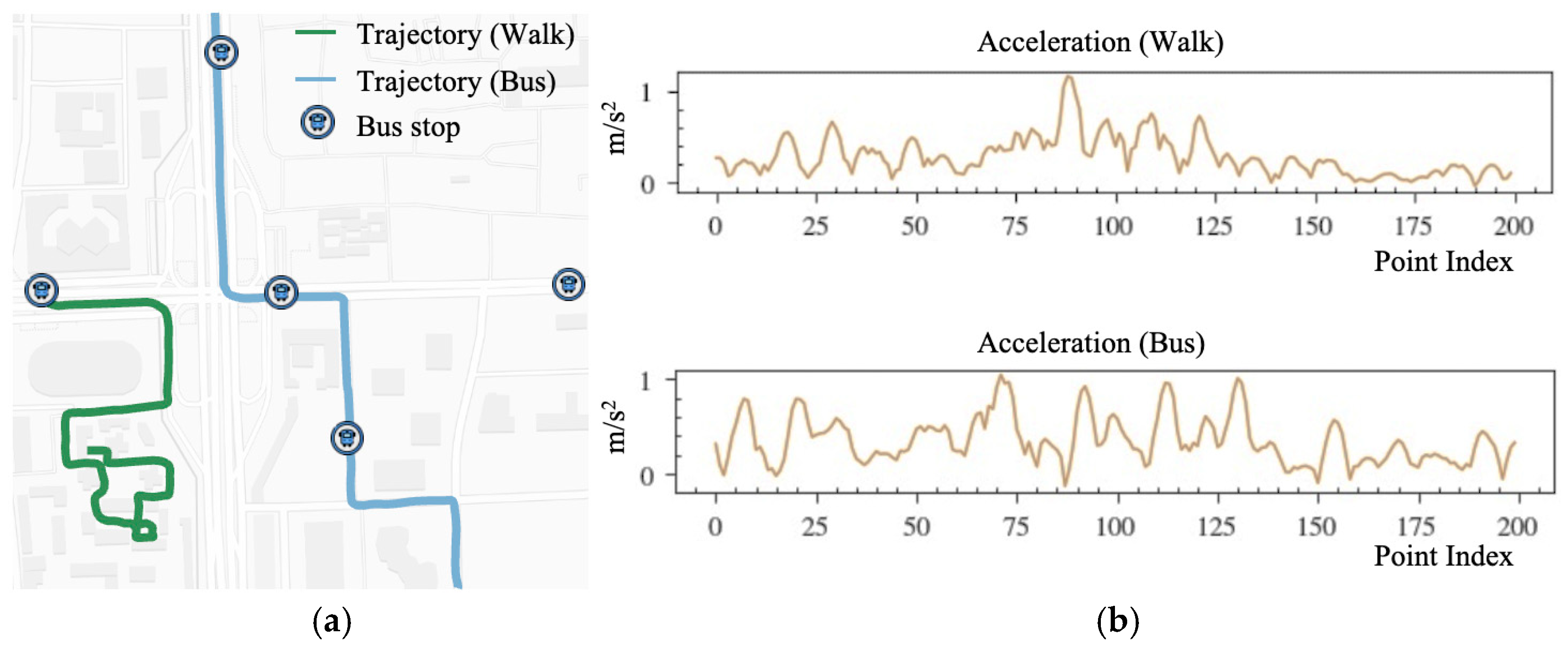
Spatial and kinematic views of trajectory data are inherently complementary in real-world scenarios. For example, while cars and buses may exhibit similar spatial distributions along urban roads, buses tend to have slower average speeds due to frequent stops. Similarly, during peak hours, vehicles and pedestrians may share comparable velocities, but vehicle trajectories are linear, whereas pedestrian paths are denser and more complex. Therefore, integrating these multi-view characteristics is crucial for accurate TMI.

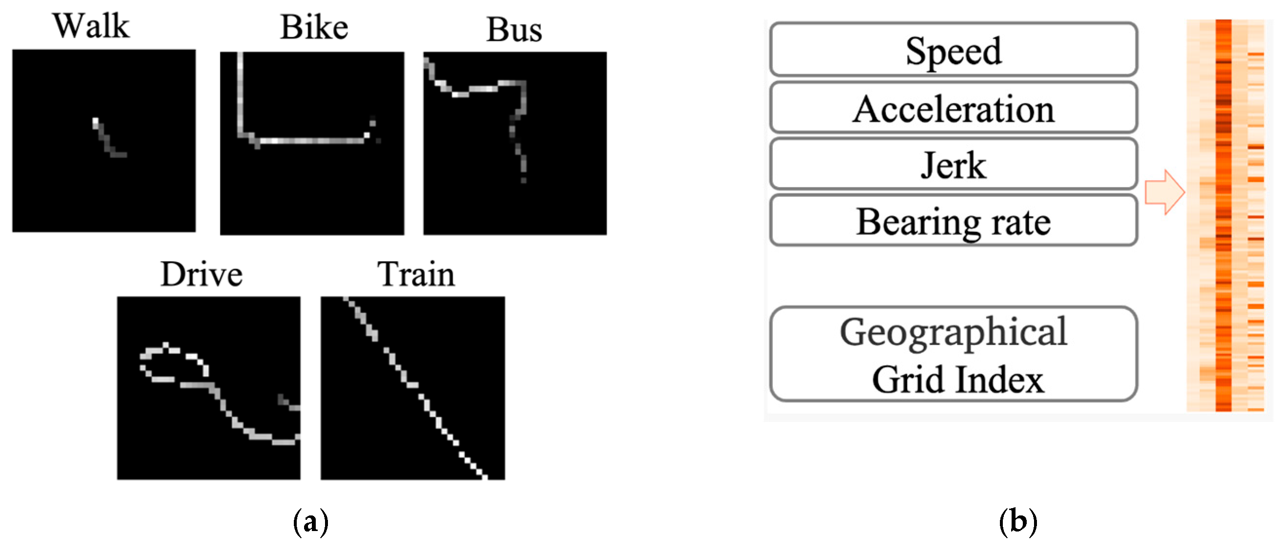
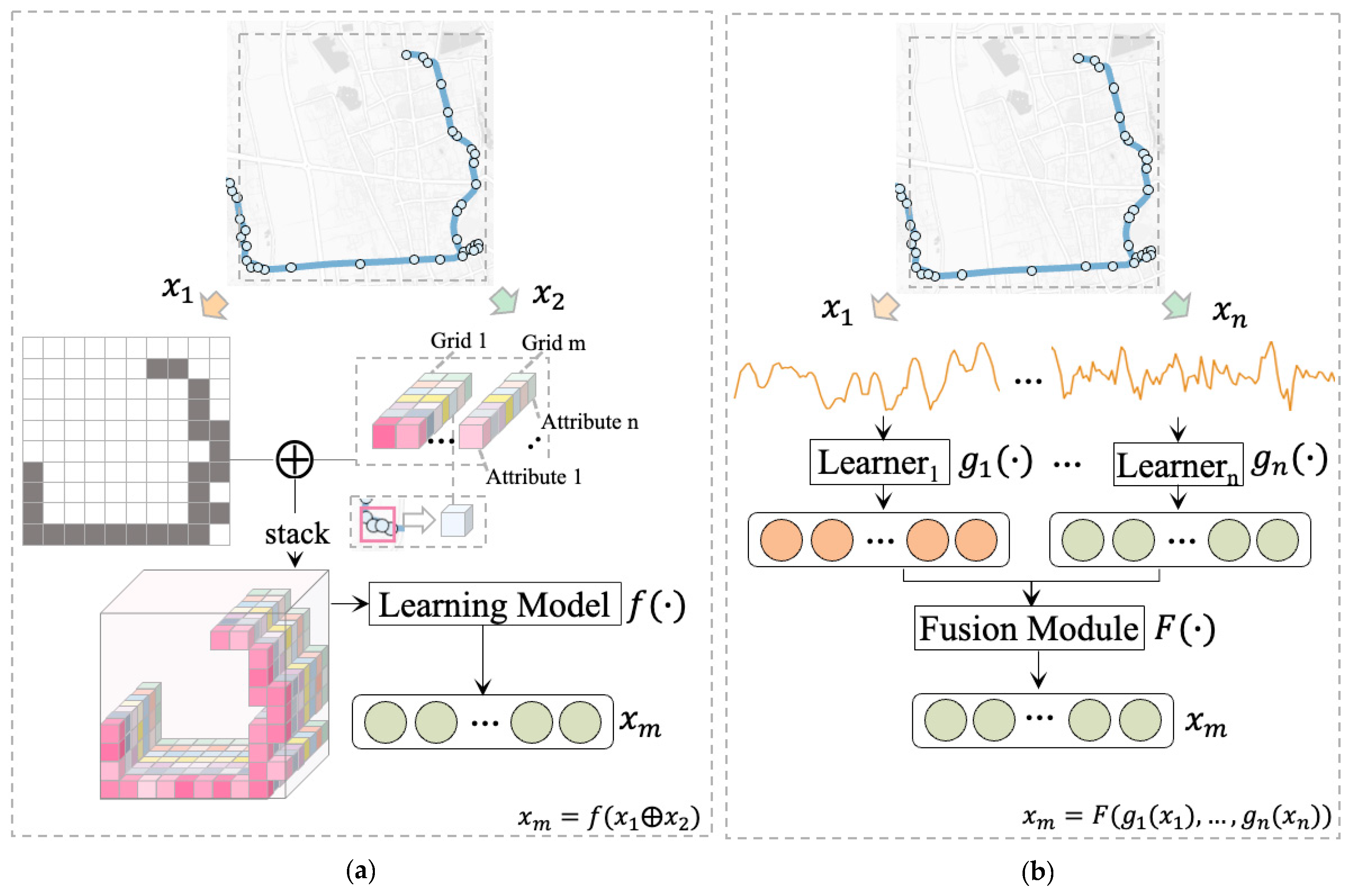
Current TMI studies primarily employ input-level fusion to integrate trajectory characteristics, combining spatial and kinematic attributes into a unified structure, often an image, before feeding them into the model for high-level feature extraction. For example, Endo et al. introduced an image-based representation where pixel values indicate the count of GPS points in each grid cell (Figure 2a) [5]. Zhang et al. utilized grids at varying temporal and spatial granularities, assigning grid values based on the time objects spent within each grid [7,8]. Ma et al. enhanced this approach by stacking nine kinematic attributes with projected pixels to create a higher-dimensional representation of spatial and kinematic features [6]. Nawaz et al. concatenated geographical region indices with kinematic attributes to form composite input records (Figure 2b) [2]. However, these input-level fusion methods constrain the model’s ability to fully exploit complementary information across views due to the rigid input structure and uniform feature extraction process for both views. In contrast, available feature-level fusion methods exhibit great potential in effective feature alignment and can be used to facilitate TMI with complementary view features, but they remain largely unexplored in current TMI research.

Based on the identified limitations, we propose multi-view contrastive fusion (MVCF)-TMI, a novel TMI framework that employs multi-view contrastive learning. The key contributions of this work are as follows:

(1) We introduce a comprehensive framework that integrates fine-grained spatial patterns and detailed kinematic attributes from GPS trajectories, enabling efficient and accurate TMI tasks.

(2) We introduce a novel feature-level fusion mechanism that aligns spatial and kinematic views within a shared subspace to produce a more discriminative trajectory representation and uncover deeper spatiotemporal semantic correlations between the views.

Furthermore, extensive evaluations on a large-scale public GPS trajectory dataset demonstrate the proposed method’s effectiveness and robustness. Additional experiments highlight MVCF-TMI’s ability to utilize both labeled and unlabeled data, supporting its application in self-supervised and supervised pretraining paradigms.

2. Related Work

While recent studies have explored incorporating smartphone sensor data (e.g., accelerometers and gyroscopes) to enhance TMI accuracy [12,13,14,15,16,17,18,19], our work focuses specifically on GPS trajectory data due to its universal availability and ability to provide sufficient spatial–kinematic information without additional sensor dependencies [1,20,21]. Consequently, in our literature review, we prioritize works that adopt the same data kind and examine three key aspects: (1) feature engineering from raw GPS data; (2) fusion of spatial and kinematic attributes in TMI; and (3) multi-view learning methods for fusing different data views.

2.1. Feature Engineering of GPS Trajectories

Feature engineering involves extracting meaningful characteristics from raw GPS points to improve model performance. In TMI, this process typically emphasizes two key dimensions: deriving kinematic attributes and identifying spatial patterns within GPS trajectories.

(1) Calculation of kinematic attributes: Kinematic attributes derived from GPS data characterize kinematic states, such as distance, velocity, acceleration, jerk, and bearing rate [3,22,23,24,25]. Two primary approaches are used to calculate these attributes:

(i) Point-level kinematic attributes are calculated from consecutive GPS points, including attributes such as point-wise distance, duration, velocity, acceleration, jerk, bearing, and bearing rate [2,3,10,22,26,27,28,29,30,31,32,33,34,35];

(ii) Segment-level attributes are computed from entire trajectories or trajectory segments, providing aggregate statistics such as total distance, average acceleration, and maximum speed [36]. These attributes also include statistical measures (e.g., the mean, variance, percentile, interquartile range, skewness, and kurtosis [37]) of point-level features, along with higher-order kinematic characteristics like rate of heading change, speed change, and stops [38,39,40,41,42,43,44,45].

(2) Capture of spatial patterns: Approaches for capturing spatial patterns in GPS trajectories are categorized into three main types: location, graph, and image-based methods (Table 1):

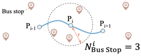
(i) Location-based methods use geographical information to represent travel patterns, such as the distance between GPS points, the nearest subway station, or the number of bus stops within a defined radius [3,28,32,40,46,47,48]. While effective, these methods require additional datasets, such as road networks and points of interest (POI), increasing the complexity of data preprocessing;

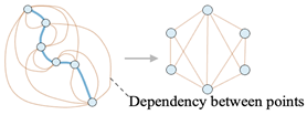
(ii) Graph-based approaches model spatial correlations between GPS points as edges in a structured graph [49,50]. This method excels at capturing long-range trajectory dependencies but is computationally intensive and demands significant memory resources, especially for large-scale trajectory datasets.

Table 1. Summary of spatial feature construction in previous research.

Categories	Related Studies	Example Illustration
Location-based	[3,28,32,40,46,47,48]
Graph-based	[49]
Image-based	[5,6,7,8,51,52]

Table 1. Summary of spatial feature construction in previous research.

Categories	Related Studies	Example Illustration
Location-based	[3,28,32,40,46,47,48]
Graph-based	[49]
Image-based	[5,6,7,8,51,52]

(iii) Image-based methods: Recent developments in trajectory analysis have focused on transforming GPS data into image representation at various scales and sizes to directly capture spatial distribution patterns. Endo et al. introduced an approach that clipped trajectories within a fixed spatial range and projected them onto uniformly sized images [5]. Building on this, Zhang et al. mapped trajectories into images with varying spatial and temporal granularities [7,8], improving the TMI of GPS tracks. Ma et al. further advanced this concept by projecting trajectories onto different image sizes across multiple spatial scales [6], capturing complex spatial distributions more effectively.

Both types of features offer distinct advantages for TMI. Kinematic attributes excel at capturing kinematic states, while spatial features provide insights into geographical context. However, most existing methods emphasize only one feature type, which may limit their ability to fully analyze trajectory characteristics.

2.2. Feature Fusion Methods

Feature fusion refers to the process of combining different feature representations extracted from data sources to create more informative and discriminative representations. In the context of deep learning, it involves strategically integrating features from multiple sources or layers to enhance the model’s ability to capture complex patterns and relationships [53]. It can occur at various levels, e.g., input-level or feature-level, with input-level fusion being the most commonly explored in current TMI studies.

(1) Input-level Fusion: This method combines spatial patterns and kinematic attributes into a simple structure before high-level feature learning. For example, Nawaz et al. concatenated geographic region indices with kinematic attributes [2], while Ma et al. introduced a multi-attribute image structure (Figure 3a) that maps detailed kinematic attributes onto spatial cells [6]. While input-level fusion effectively integrates trajectory characteristics, it often fails to capture intricate inter-view relationships, limiting its ability to fully leverage complementary spatiotemporal information in GPS data.

(2) Feature-level fusion: Unlike input-level fusion, feature-level fusion processes data through independent sub-learners to generate view-specific representations, which are then combined using a fusion module to create a compact and informative joint latent representation (Figure 3b). This approach enables deeper interaction between modalities, capturing complementary information while minimizing redundancy and noise. It has demonstrated effectiveness across domains. For example, in human action recognition, depth, skeleton, and accelerometer features are fused to represent spatiotemporal dynamics, improving recognition accuracy [54,55,56,57]. In multimodal language models, such as BLIP-2 [58] and LLaMA-Adapter [59], visual features are integrated with text embeddings through methods, such as Q-Former or MLP-based connectors, enhancing vision–language understanding [60]. Similarly, remote sensing leverages feature-level fusion of spatial and spectral data, followed by a prediction head, to improve land-use and land-cover classification [61]. Despite its success in various fields, feature-level fusion remains underutilized in TMI research, representing a promising area for further exploration.

Both input- and feature-level fusion strategies seek to integrate multiple features, yet they differ in how and when this integration occurs. The following section explores how contrastive learning can further enhance feature-level fusion by explicitly aligning complementary views in a shared feature space.

2.3. Multi-View Contrastive Learning

Multi-view learning integrates diverse data perspectives into a shared feature space, typically with feature-level fusion capturing complementary information, enabling more discriminative representations than single-view methods [62,63,64,65]. The single-view methods use a single data type or concatenate multiple features into a unified input, following a learning setup similar to input-level fusion (as described in Section 2.2) [61,66,67].

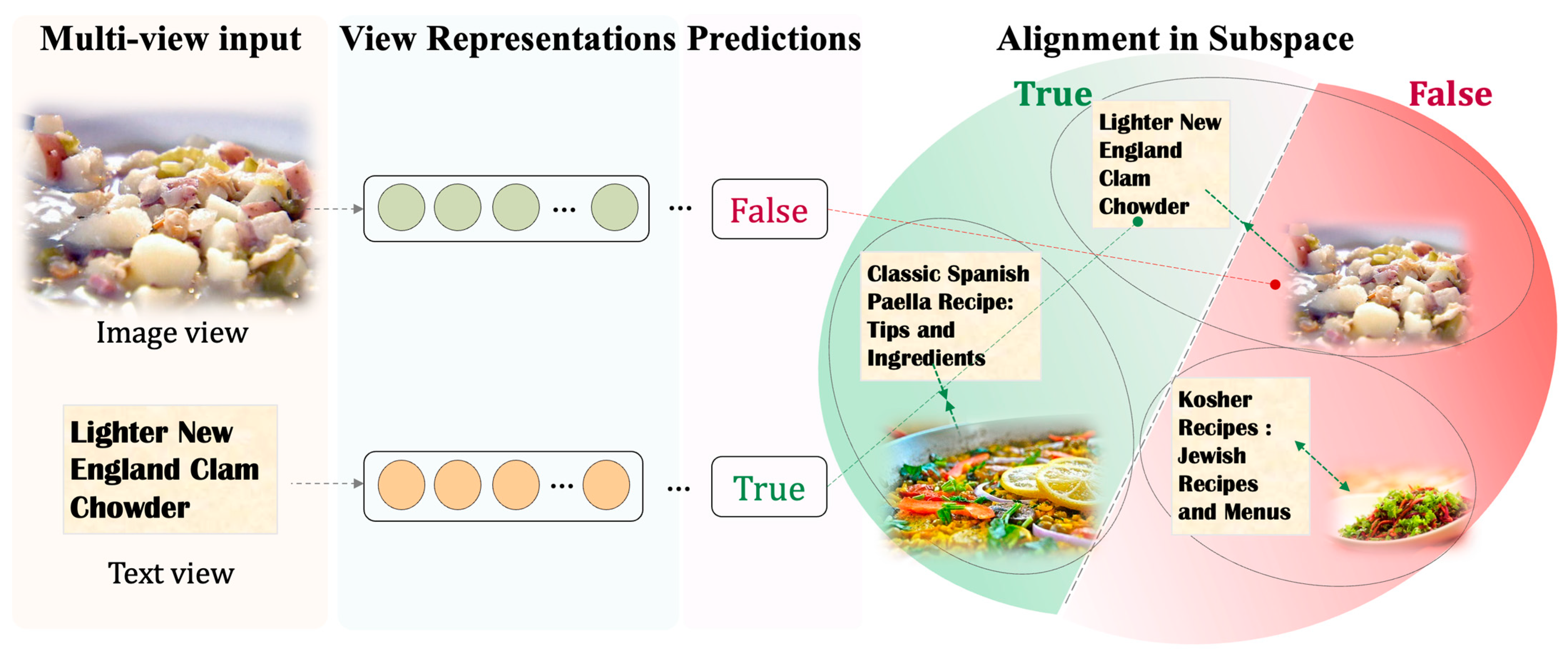
The “multi-view” concept encompasses diverse inputs, such as multimodal (Figure 4), multisource, multi-sensor data [61], and multi-view features [68], which describe distinct characteristics derived from the same dataset [66,67,69,70]. Examples include shape and edge features extracted from handwritten numerals [71,72], or temporal, spatial, and semantic attributes of taxi request data [73].

Common methodologies in multi-view learning include Canonical Correlation Analysis (CCA)-based methods, deep subspace clustering, and contrastive learning [74]. These techniques have shown efficacy in domains such as image classification, natural language processing, and human activity recognition (HAR) [71,72,75,76].

Contrastive learning refines multi-view learning by aligning and fusing features through the differentiation of similar and dissimilar samples [77,78]. By modeling complex inter-view relationships and ensuring consistency in representations, it outperforms traditional methods, such as CCA [62,64] in capturing high-level associations. Multi-view applications utilize views of the same data to form positive and negative pairs, enabling robust and transferable representation learning [79,80].

This adaptable technique has been effectively utilized in diverse fields, including clustering [81], point-cloud analysis [82], and image classification [83], leveraging complementary information across multiple views. For example, Zou et al. aligned multimodal representations on a sample basis to improve inter-modal correspondence for accurate predictions [83] while distinguishing incorrect ones (Figure 4). Similarly, Si et al. augmented trajectories and applied contrastive loss to capture more detailed mobility patterns [84]. Li et al. introduced TrajRCL [85], employing trajectory augmentation to produce low-distortion, high-fidelity views and enhance consistency in trajectory representations through self-supervised contrastive learning objectives.

Despite the above progress, multi-view contrastive learning frameworks in TMI applications remain unexplored, particularly those that incorporate both trajectory kinematic attributes and spatial patterns as complementary views in deep learning models.

3. Preliminaries

This section presents the notation used in this study (

Table 2. Definitions of the notations.

Notation	Definition
$P_i$	The $i^{th}$ GPS point, defined by attributes: latitude ($la{t}_i$), longitude ($ln{g}_i$), and timestamp ($t_i$). Optionally, it includes a mode label: $P_i=(la{t}_i, ln{g}_i, { t}_i, mod{e}_i)$.
$T_r$	A GPS trajectory consisting of a sequence of time-stamped, consecutive GPS points: $T_r=(P_1, P_2, \dots , P_i, \dots , P_N)$. $N$ is the number of GPS points.
${Seg}_i$	The $i^{th}$ GPS segment, partitioned from trajectories and corresponding to a unique travel mode: ${Seg}_i=(P_1, P_2,\dots , P_i,\dots P_N,mod{e}_i)$.
$F_{im}$	The $m^{th}$ feature type extracted from ${Seg}_i.$
$mod{e}_i$	The $i^{th}$ travel mode.
$L$	The length of each fixed-length trajectory segment.
$X_{\mathrm{Kinematics}}$	The input instances for the kinematic view.
$X_{\mathrm{Image}}$	The total input instances for the spatial view.
$x_{{\mathrm{i}\mathrm{m}\mathrm{a}\mathrm{g}\mathrm{e}}_{\mathrm{k},\mathrm{j}}}$	The tensor corresponding to the $j^{th}$ scale and $k^{th}$ object instance of the spatial view.
${\mathcal{F}}_{{\theta }_a^i}(·)$	A subnetwork designed to extract features from $x_{{\mathrm{i}\mathrm{m}\mathrm{a}\mathrm{g}\mathrm{e}}_{k,i}}$, where ${\theta }_a^i$ represents its learnable weights.
${\mathcal{G}}_{{\theta }_b}(·)$	A subnetwork designed to extract features from $X_{\mathrm{Kinematics}}$, where ${\theta }_b$ represents its learnable weights.
$c_{\varphi }$	The classification module responsible for the view-specific classification and the final classification for the travel mode, where$\varphi$ denotes its learnable weights.
$h_{a_{kj}}$	The feature vector extracted from the input tensor $x_{{\mathrm{i}\mathrm{m}\mathrm{a}\mathrm{g}\mathrm{e}}_{\mathrm{k},\mathrm{j}}}$ by the subnetwork ${\mathcal{F}}_{{\theta }_a^j}(·)$.
${\mathrm{H}}_{a_{\mathrm{j}}}$	The concatenated feature vector of {$h_{a_{1j}},h_{a_{2j}},\dots ,h_{a_{Kj}}$}.
${\mathrm{H}}_b$	The feature vector extracted from the input tensor $X_{\mathrm{Kinematics}}$ by the subnetwork ${\mathcal{G}}_{{\theta }_b}(·)$.
${\mathrm{H}}_{\mathfrak{m}}$	The fused multi-view feature vector.

) and outlines the research problem.

Problem Statement. The objective of TMI is to determine the modes of transport within a given trajectory $T_r$. Each trajectory represents the movement of a single traveler and may encompass multiple transitions between transportation modes. Building on previous TMI research [6,10], we focused on identifying five modes of transport: walking, bus, cycling, driving, and train. To achieve this purpose, the trajectory was divided into discrete segments. Each segment is represented by ${Seg}_i$, and $m$ types of attributes extracted from the raw trajectory for ${Seg}_i$ are denoted as {$F_{i1}, F_{i2}, \dots , F_{im}\}$. The problem was then formulated as follows: given a segment ${Seg}_i$, we first extract its attribute sets and train a framework $F(·)$ to classify the segment by transportation mode, as expressed in Equation (1).

$${\mathrm{S}\mathrm{e}\mathrm{g}}_{\mathrm{i}}=\left\{F_{i1},F_{i2},\dots ,F_{im}\right\}\stackrel{F\left(·\right)}{\to }mod{e}_i$$

(1)

4. Method

4.1. Overview

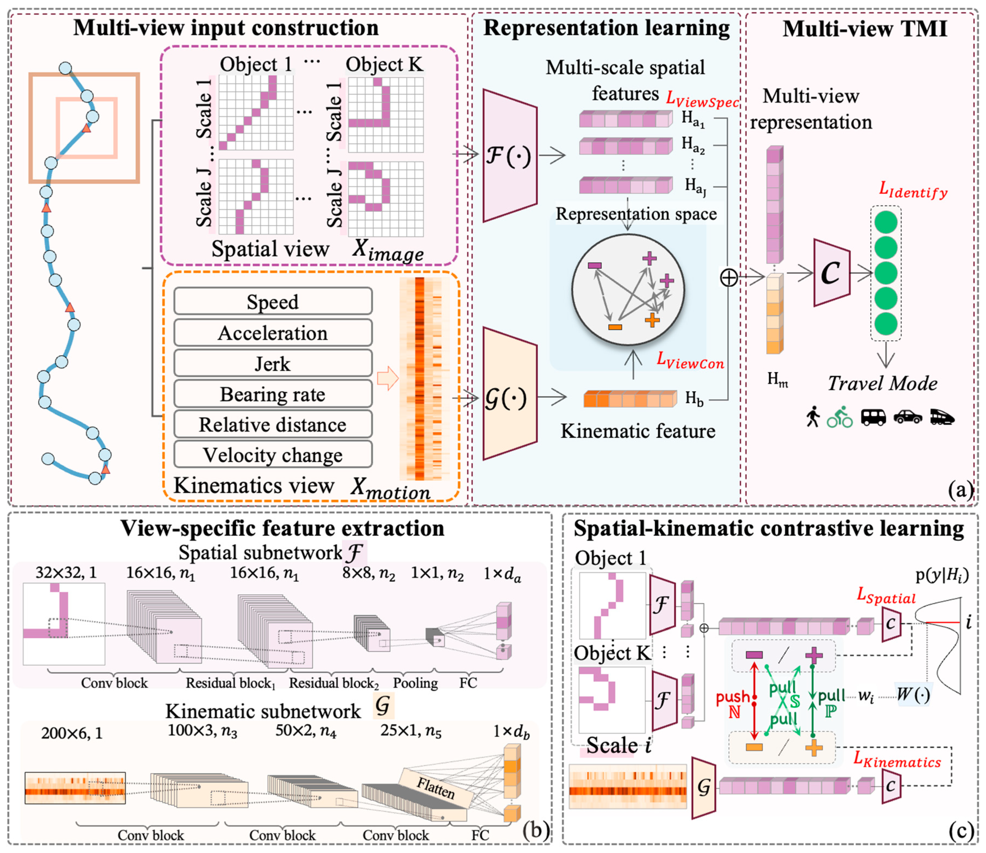
The MVCF-TMI framework consists of four primary steps:

(1) Multi-view input construction: Raw trajectory data are processed into structured spatial and kinematic inputs through point-to-image projection and pointwise attribute calculation, depicted in the left panel of Figure 5a.

(2) View-specific feature extraction: Two specialized Convolutional Neural Network (CNN) subnetworks are employed to extract high-dimensional features independently from each view (Figure 5b).

(3) Spatial–kinematic contrastive learning: A contrastive learning module aligns the features from both views, leveraging view-specific classification results for guidance (Figure 5c).

(4) Fusion and joint learning: The fused multi-view representations are utilized for the final TMI task (Figure 5a). The model training minimizes a joint loss function that combines contrastive loss, final TMI loss, and view-specific losses.

4.2. Multi-View Input Construction

4.2.1. Kinematic View Construction

After preprocessing the data (Section 5.1.3), the raw trajectory data were divided into a collection of fixed-length L segments, $Se{g}_i=\{P_1,\dots ,P_L\} \left(i=1,\dots ,n\right)$, where $n$ represents the total number of segments. For each segment, six kinematic attributes were calculated for every two consecutive points along the temporal dimension (Figure 5a), producing input instances $X_{\mathrm{Kinematics}}\in {\mathbb{R}}^{N\times 1\times L\times 6}$, with $N$ indicating the batch size.

To construct the kinematic view, we utilized standard point-level kinematic attributes of GPS data from TMI. Equations (2)–(6) define the calculations for relative distance, speed, velocity change, acceleration, and jerk at each point $P_i$.

$$d_i=Vincenty(P_i,P_{i+1})$$

(2)

$$v_{p_i}={\displaystyle \frac{d_i}{t_{i+1}-t_i}}$$

(3)

$$\Delta v_i=\left|{\nu }_{i+1}-{\nu }_i\right|$$

(4)

$$a_{p_i}={\displaystyle \frac{\Delta v_i}{t_{i+1}-t_i}}$$

(5)

$$j_{p_1}={\displaystyle \frac{a_{p_{i+1}}-a_{p_i}}{t_{i+1}-t_i}}$$

(6)

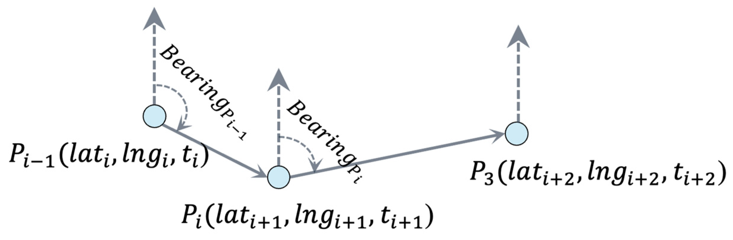
To identify transportation modes, we analyzed directional change patterns by calculating the bearing (directional angle of movement) between consecutive GPS points and their rate of change. This metric distinguishes movement types: trains exhibit minimal directional variation due to fixed tracks, buses and cars demonstrate moderate changes along roadways, and pedestrians frequently and abruptly alter direction. Given two GPS coordinates $(la{t}_i, ln{g}_i)$ and $({lat}_{i+1}, {lng}_{i+1})$, the bearing was computed using Equations (7)–(9) (Figure 6), while the bearing rate was derived using Equation (10).

$$y=\sin \left({lng}_{i+1}-{lng}_i\right)\times \cos \left(la{t}_{i+1}\right)$$

(7)

$$x=cos\left(la{t}_i\right)\times sin\left(la{t}_{i+1}\right)-sin\left(la{t}_i\right)\times cos\left(la{t}_{i+1}\right)\times cos(ln{g}_{i+1}-ln{g}_i)$$

(8)

$$Bearin{g}_{Pi}=\mathrm{a}\mathrm{r}\mathrm{c}\mathrm{t}\mathrm{a}\mathrm{n}\left(y,x\right)$$

(9)

$$Bearing Rat{e}_{Pi}=\left|Bearin{g}_{P_{i+1}}-Bearin{g}_{P_i}\right|$$

(10)

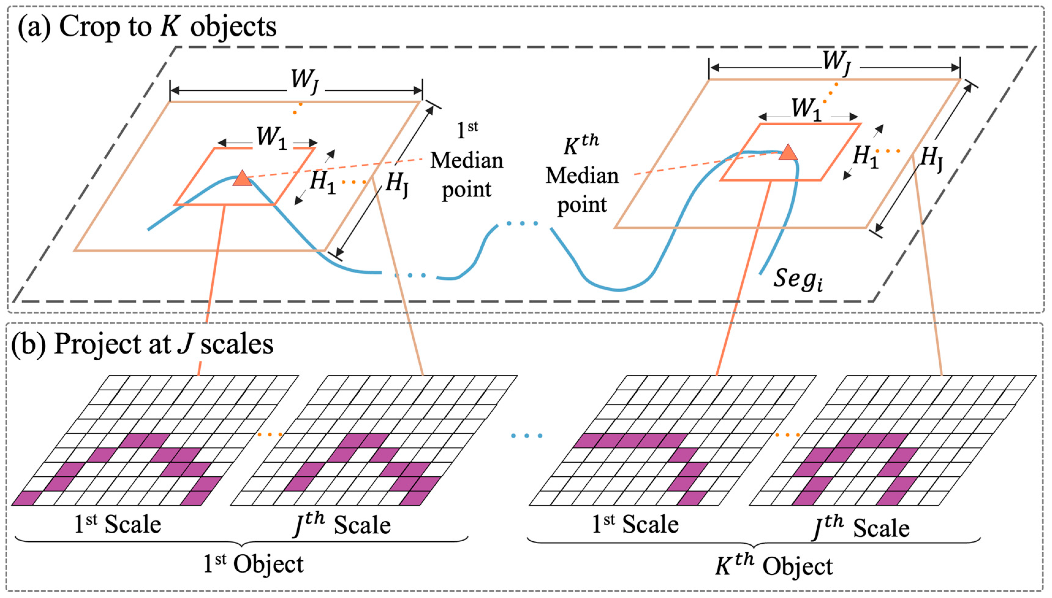
4.2.2. Spatial View Construction

To generate multiscale trajectory images from a trajectory segment ${\mathrm{S}\mathrm{e}\mathrm{g}}_i$, we applied the method proposed by [6], which projects ${\mathrm{S}\mathrm{e}\mathrm{g}}_{\mathrm{i}}$ onto images at multiple geographical scales to capture the spatial distribution features of trajectories. Each segment ${\mathrm{S}\mathrm{e}\mathrm{g}}_{\mathrm{i}}$ was first divided into $K$ subsegments, termed “objects” (Figure 7a). Next, each object was projected onto a series of images at $J$ geographical scales, using the median point of the subsegment as the image center (Figure 7b). The projection utilized a geographical window defined by width $W$ and height $H$ in degrees.

Our current implementation assigned feature values only to grid cells containing GPS points, ensuring a direct representation of the observed trajectory without interpolation. Note that smaller geographical windows may naturally result in sparser representations, reflecting the inherent spacing of trajectory points.

The process was formalized in the equations below.

$$\begin{gathered} \mathrm{S}\mathrm{e}{\mathrm{g}}_i \stackrel{\mathrm{divide}}{\underset{K}{\to }} \{\mathrm{O}\mathrm{b}\mathrm{j}\mathrm{e}\mathrm{c}{\mathrm{t}}_1, \dots ,\mathrm{O}\mathrm{b}\mathrm{j}\mathrm{e}\mathrm{c}{\mathrm{t}}_K\} \\ \mathrm{O}\mathrm{b}\mathrm{j}\mathrm{e}\mathrm{c}{\mathrm{t}}_i\stackrel{\mathrm{project}}{\underset{\begin{array}{c}{s}_1: \left[W_1\times H_1\right]\\ s_2: \left[W_2\times H_2\right]\\ \dots \\ s_J: [W_J\times H_J]\end{array}}{\to }}\{\mathrm{i}\mathrm{m}\mathrm{a}\mathrm{g}{\mathrm{e}}_1,\dots ,\mathrm{i}\mathrm{m}\mathrm{a}\mathrm{g}{\mathrm{e}}_J\} \end{gathered}$$

We also directly used the optimal parameter settings from [6]: ($K=4$, $J=3$, and an image size $of 32\times 32$). For the geographic scale size, we optimized accuracy through grid search, selecting [0.0007$°$ × 0.0007$°$], [0.003$°$ × 0.003$°$], and [0.07$°$ × 0.07$°$] as the optimal values. Each grid’s pixel value was assigned as the average speed of the GPS points within that grid. The resulting input instance for the spatial view was represented as $X_{\mathrm{Image}}\in {\mathbb{R}}^{N\times J\times K\times 1\times 32\times 32}$, where $N$ denotes the batch size.

4.3. View-Specific Feature Extraction

Feature extraction was conducted using a dual-stream network architecture comprising a spatial subnetwork $\mathcal{F}(·)$ and a kinematics subnetwork $\mathcal{G}(·)$. These networks transformed the spatial distribution and kinematic attributes of the trajectories into high-dimensional embeddings (Figure 5b).

Table 3. Structure of the two subnetworks.

Modules	Blocks	Layers
Kinematics subnetwork	Convolutional block × 3	([1 × 3] conv → ReLU → [1 × 3] conv → ReLU → [1 × 2] MaxPool2d) × 3
	Fully connected block	Flatten → Fully connected → ReLU
Spatial subnetwork	Shallow convolutional block	[3 × 3] conv → BatchNorm2d → ReLU → [3 × 3] MaxPool2d
	Residual block	[3 × 3] conv → BatchNorm2d → ReLU → [1 × 1] conv → BatchNorm2d (Skip connection) → ReLU
	Pool block	[2 × 2] AvgPool2d
	Residual block	[3 × 3] conv → BatchNorm2d → ReLU → [1 × 1] conv → BatchNorm2d (Skip connection) → ReLU
	Fully connected block	Flatten → Fully connected → ReLU

details the structure of the two subnetworks. The $\mathcal{F}(·)$ processed a single image $x_{{\mathrm{i}\mathrm{m}\mathrm{a}\mathrm{g}\mathrm{e}}_{\mathrm{k},\mathrm{j}}}\in {\mathbb{R}}^{1\times 32\times 32}$, corresponding to the $k^{th}$ object at scale $j$. The image passed through a convolutional layer, two residual blocks, and was mapped to a feature vector $h_{a_{kj}}\in {\mathbb{R}}^{1\times d_a}$ via pooling and a fully connected layer, as defined in Equation (13). The optimized $\mathcal{G}(·)$ based on the CNN configuration from [10], extracted kinematic features using three stacked convolutional blocks, each comprising two convolutional layers with ReLU activation. Pooling and fully connected layers then mapped the output to a high-dimensional feature vector $H_b\in {\mathbb{R}}^{1\times d_b}$, as described in Equation (12).

The concatenated feature vectors from all objects at scale $j$ are defined in Equation (11) and serve as the output of the image feature extraction process. These concatenated features were subsequently utilized in contrastive learning (Figure 5c).

$${\mathrm{H}}_{{\mathrm{a}}_{\mathrm{j}}}\in {\mathbb{R}}^{1\times \left(d_a\ast K\right)}=h_{{\mathrm{a}}_1}\oplus h_{{\mathrm{a}}_2}\oplus \dots \oplus h_{{\mathrm{a}}_{\mathrm{K}}}(j=1,\dots J;d_a\ast K\stackrel{\scriptscriptstyle\mathrm{def}}{=}{d}_b)$$

(11)

$${\mathrm{H}}_b={\mathcal{G}}_{{\theta }_b}\left(X_{\mathrm{Kinematics}}\right)\in {\mathbb{R}}^{1\times d_b}$$

(12)

$$h_{a_{kj}}={\mathcal{F}}_{{\theta }_a^i}\left(x_{\mathrm{I}\mathrm{m}\mathrm{a}\mathrm{g}{\mathrm{e}}_{kj}}\right)\in {\mathbb{R}}^{1\times d_a},j=1,\dots ,J;k=1,\dots K$$

(13)

where ${\theta }_a^i$ and ${\theta }_b$represent the weights of the view-specific subnetwork ${\mathcal{F}}_{{\theta }_a^i}(·)$ and kinematics view-specific subnetwork ${\mathcal{G}}_{{\theta }_b}(·)$, respectively. It is important to note that the encoders for the spatial view at different image scales were trained independently. Their weights and biases were optimized for the specific scale of image samples, allowing the encoder to adapt effectively to feature extraction across varying spatial ranges.

4.4. Spatial–Kinematic Contrastive Learning

Spatial–kinematic contrastive learning integrates kinematic and multiscale spatial trajectory features into a unified subspace, generating a semantically rich, shared representation that captures complementary spatial and kinematic characteristics. First, the effectiveness of view-specific features was assessed using supervised multilayer perceptron (MLP) classifiers, with a total view-specific loss defined via cross-entropy. Subsequently, guided by this loss, three types of sample pairs were used to define a weighted contrastive loss function. This function aligned view-specific representations, enabling the model to learn comprehensive and effective feature representations.

4.4.1. View-Specific Classification

View-specific classification using MLP classifiers evaluates the effectiveness of the extracted spatial and kinematic features by assessing their ability to distinguish between different traffic modes. A view-specific classification task was designed to optimize these features. Based on the classification results, pairs were categorized as inter-view positive, semi-positive, or negative, guiding subsequent contrastive learning processes.

As described in Section 4.3, the inputs for the view-specific prediction task were: ${\mathrm{H}}_{{\mathrm{a}}_{\mathrm{j}}}\in {\mathbb{R}}^{1\times \left(d_a\ast K\right)} (j=1,\dots ,J)$ and ${\mathrm{H}}_b\in {\mathbb{R}}^{1\times d_b}$. Each MLP classifier served as a probabilistic model $c_{\varphi }:\mathcal{H}\to \mathcal{P}$, mapping the view-specific hidden representation to a predictive distribution $p\left(y\right|H)$. The aim of the view-specific classification task was to minimize the prediction loss for each view, calculated using cross-entropy loss. The total loss ${\mathcal{L}}_{\mathrm{ViewSpec}}$ was computed as the weighted sum of spatial and kinematic view losses, balanced by the hyperparameter $\lambda$, as expressed in Equations (14)–(16):

$${\mathcal{L}}_{\mathrm{Spatial}}={\displaystyle \frac{1}{J}}{\sum }_{i=1}^J(-{\sum }_{r=1}^R{y}^r\log p_a^{i,r}),$$

(14)

$${\mathcal{L}}_{\mathrm{Kinematics}}=-{\sum }_{r=1}^R{y}^r\mathrm{l}\mathrm{o}\mathrm{g}{p}_b^r,$$

(15)

$${\mathcal{L}}_{\mathrm{ViewSpec}}={\mathcal{L}}_{\mathrm{Spatial}}+\mathsf{\lambda }{\mathcal{L}}_{\mathrm{Kinematics}},$$

(16)

where $\mathsf{\lambda }$ balances the contributions from both views in the total loss computation. The loss for the spatial view was derived using J independent classifiers $c_{{\varphi }_a^i} (i=1,\dots ,J)$. $y^r$ indicates the $r^{th}$ ground truth travel mode label, encoded as a one-hot vector indicating the correct class. The softmax output for the spatial view at scale $i$ is denoted as $[p_a^{i,1};p_a^{i,2};...;p_a^{i,R}]={\mathrm{p}}_a\left(y|H_a^i\right)$, while the softmax output for the kinematic view feature is represented as $p_b^r{=\mathrm{p}}_b\left(y|H_b\right)$.

4.4.2. Inter-View Contrastive Learning

Using the view-specific classification results, we extended pair definition in [83] to kinematic and spatial trajectory views, categorizing pairs as positive, semi-positive, or negative (denoted as $\mathbb{P},\mathbb{N},\mathbb{S}$). These definitions are detailed in Equations (17)–(19) and illustrated in (Figure 5c).

$$\mathbb{P}={\left\{n\mid {\widehat{y}}_{a,n}^j\equiv y_n \mathrm{a}\mathrm{n}\mathrm{d} {\widehat{y}}_{b,n}\equiv y_n\right\}}_{n=1}^N,$$

(17)

$$\mathbb{N}={\left\{n\mid {\widehat{y}}_{a,n}^s\ne y_n \mathrm{a}\mathrm{n}\mathrm{d} {\widehat{y}}_{b,n}\ne y_n\right\}}_{n=1}^N,$$

(18)

$$\mathbb{S}=\{n\mid {\widehat{y}}_{a,n}^s\equiv y_n \mathrm{and} {\widehat{y}}_{b,n}\ne y_n{\}}_{n=1}^N\cup \{n\mid {\widehat{y}}_{a,n}^s\ne y_n \mathrm{and} {\widehat{y}}_{b,n}\equiv y_n\},$$

(19)

where $N$ represents the batch size. The predicted result for the spatial view’s $n^{th}$ sample at $j^{th}$ scale, ${\widehat{y}}_{a,n}^j$, was obtained as ${\mathrm{H}}_{a,n}^j\to {\widehat{y}}_{a,n}^j$. Similarly, ${\widehat{y}}_{b,n}$ denotes the kinematic view’s $n^{th}$ sample, derived as ${\mathrm{H}}_{b,n}\to {\widehat{y}}_{b,n}$.

Inter-view contrastive learning aligns view-specific representations with their most task-relevant counterparts using three key operations:

• Maximizing similarity between positive pairs by jointly updating representations from both views;
• Minimizing similarity between negative pairs to promote complementary spatial–kinematic representations;
• Aligning incorrect representations with correct ones by detaching the correct representation from the computation graph and maximizing similarity, ensuring updates are applied only to the incorrect representation.

For each in-batch sample, spatial view features at each scale were contrasted with kinematic view features. Negative sample pairs $\mathbb{N}$ that confused both spatial and kinematic classifiers were treated as challenging cases. To address these samples, a weight factor $w_j$ (defined in Equation (20)) was introduced, increasing with the decline in the spatial feature’s efficacy. This weight emphasized negative pairs at the $j^{th}$ scale, encouraging the model to learn more complementary inter-view features. The overall inter-view contrastive loss (IVCL) was formalized in Equation (21):

$$w_j=e^{-{\sum }_{r=1}^R{y}^r\log p_a^{j,r}}$$

(20)

$${\mathcal{L}}_{\mathrm{ViewCon}}=-{\displaystyle \frac{1}{J}}{\sum }_{j=1}^J \mathrm{l}\mathrm{o}\mathrm{g} {\displaystyle \frac{\sum _{{\mathrm{z}}^{+}\in \mathbb{P}\cup \mathbb{S}} e^{\mathrm{s}\mathrm{i}\mathrm{m}\left(H_{a,{\mathrm{z}}^{+}}^j,H_{b,{\mathrm{z}}^{+}}\right)/\tau }}{\sum _{{\mathrm{z}}^{+}\in \mathbb{P}\cup \mathbb{S}} e^{\mathrm{s}\mathrm{i}\mathrm{m}\left(H_{a,{\mathrm{z}}^{+}}^{\mathrm{j}},H_{b,{\mathrm{z}}^{+}}\right)/\tau }+w_j\sum _{{\mathrm{z}}^{-}\in \mathbb{N}} e^{\mathrm{s}\mathrm{i}\mathrm{m}\left(H_{a,z^{-}}^j,H_{b,z^{-}}\right)/\tau }}}$$

(21)

where $\mathrm{s}\mathrm{i}\mathrm{m}\left(H_{a,z},H_{b,z}\right)={\displaystyle \frac{H_{a,z}·H_{b,z}}{‖H_{a,z}‖\ast ‖H_{b,z}‖}}$ is the cosine similarity between paired spatial–kinematic representations $H_{a,z}$ and $H_{b,z}$ for sample $z$, and $\tau$ is the temperature coefficient.

4.5. Fusion and Joint Learning

Following contrastive learning, we constructed a fused multi-view representation by concatenating the aligned spatial and kinematic representations. This resulted in a unified, differentiable representation, $H_m$, designed for trajectory classification. Leveraging the discriminative features obtained during the preceding process $\{H_a^1,H_a^2,\dots ,H_a^j,H_b\}$, the multi-view representation was formally defined in Equation (22):

$$H_{\mathfrak{m}}=(H_a^1\oplus \dots \oplus H_a^{\mathrm{J}})\oplus H_b$$

(22)

A classifier was subsequently applied to the fused multi-view representation to perform TMI. The associated loss is defined in Equation (23), where $p_m$ represents the probability distribution output by the multi-view classifier: $[p_m^1;p_m^2;...;p_m^R]={\mathrm{p}}_m\left(\mathrm{y}\right|H_m)$.

$${\mathcal{L}}_{Identify}=-\sum _{r=1}^R{y}^r\mathrm{l}\mathrm{o}\mathrm{g}{p}_{\mathfrak{m}}^r$$

(23)

The final joint learning objective integrated the view-specific and multi-view classification losses, and the multi-view contrastive loss, balanced using the factor $p$, as outlined in Equation (24).

$${\mathcal{L}}_{\mathrm{O}\mathrm{v}\mathrm{e}\mathrm{r}\mathrm{a}\mathrm{l}\mathrm{l}}={\mathcal{L}}_{\mathrm{ViewSpec}}+{\mathcal{L}}_{Identify}+p{\mathcal{L}}_{\mathrm{ViewCon}}$$

(24)

5. Experiments and Analyses

5.1. Experiment Datasets

To evaluate the model’s performance and generalizability, we utilized two public datasets: GeoLife and Sussex–Huawei Locomotion (SHL).

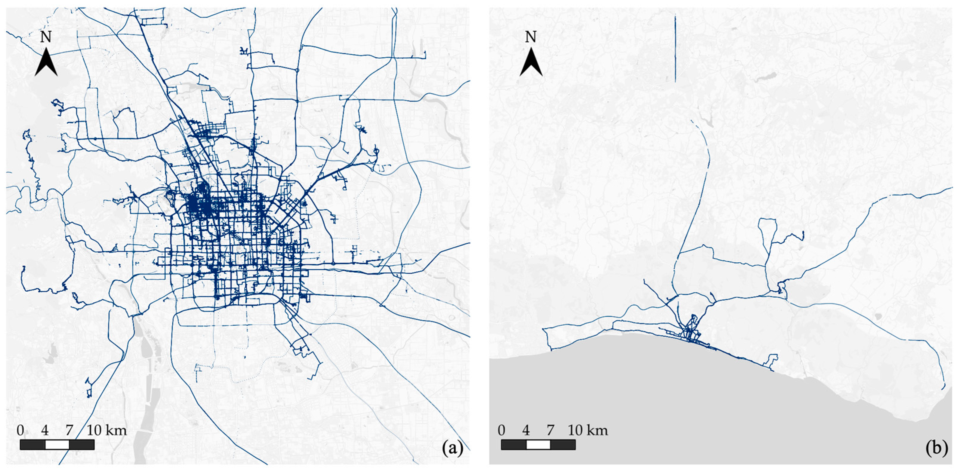
5.1.1. GeoLife Dataset

The GeoLife dataset [38,39] comprises real-world GPS trajectories collected between April 2007 and August 2012, with sampling intervals ranging from 1 to 5 s. Primarily captured in Beijing, China, it provides high-resolution data (Figure 8a). It contains 17,621 trajectories spanning a total distance of 1,292,951 km over 2090 days, engaging 182 users, of which 69 provided labeled trajectory segments specifying transportation modes. The labeled trajectories serve as the ground truth for supervised learning. Ground-level travel modes included: walking, cycling, bus, driving, and transit, consistent with prior work [10].

5.1.2. SHL Dataset

The SHL dataset [86] is a public dataset designed for HAR, particularly for TMI. It was collected over seven months in the United Kingdom by volunteers across eight transportation modes, including still, walk, run, bike, car, bus, train, and subway. We used the GPS signal from the ‘Torso’ sensor to align with the framework’s focus on GPS data. The SHL dataset contains 2812h of labeled data across these eight activities. However, for consistency with the GeoLife dataset, we selected five common transportation modes: walking, cycling, bus, driving, and train. As shown in Figure 8, the SHL dataset is significantly smaller and sparser than GeoLife, with only 344 segments remaining after preprocessing compared to 16,917 in GeoLife. The size and sample count for the five selected modes in the preprocessed SHL and GeoLife datasets are shown in

Table 4. The size and number of segments of the preprocessed GeoLife and SHL dataset.

Transportation Mode	Number of Segments (GeoLife)	Number of Segments (SHL)
Walk	5836	103
Bike	2696	45
Bus	3818	55
Driving	2515	87
Train	2042	54

. Figure 9 illustrates the distribution of travel modes across both processed datasets, highlighting these differences in data density and representation.

5.1.3. Data Preprocessing

Following the approach in [10], we preprocessed raw GPS data by dividing trajectories into trips with no point interval exceeding 20 min and splitting multi-mode segments at transition points. The resulting labeled trips, consisting of 5,494,723 GPS points, were then segmented into fixed-length (200-point) single-mode travel segments. Unrealistic GPS points and segments with fewer than 20 consecutive GPS points were discarded. Features were constructed as outlined in Section 4.2, followed by data augmentation using random horizontal and vertical image flipping and z-score normalization. This process resulted in 16,907 single-mode GPS trajectory segments, distributed among transportation modes, as shown in Table 4. The dataset was randomly split into training and test sets at a 4:1 ratio.

5.2. Experimental Settings

5.2.1. Metrics

Here, TMI was treated as a classification task, and performance was evaluated using classification accuracy. Additionally, a confusion matrix, recall, and precision were employed for a detailed analysis of model performance.

5.2.2. Implementation Settings

All experiments were conducted on a workstation equipped with an Intel Core i7-10700 CPU @ 2.90GHz, 32 GB of memory, and an NVIDIA GeForce RTX 3090 GPU, running Ubuntu 22.04. All deep learning models were implemented in Python using the PyTorch framework (version 2.0.1).

5.2.3. Baseline Methods

To evaluate the effectiveness of the proposed multi-view feature-level contrastive fusion scheme, the following baseline models were compared:

(1) Four classical machine learning models: k-nearest neighbor (KNN), support vector machine (SVM), decision tree (DT), and random forest (RF);

(2) Two deep learning models: CNN [10] and MASO-MSF [6].

To ensure consistency, the input data for both classical and deep learning baselines was derived from MASO-MSF, incorporating spatial features and seven types of local point-level kinematic attributes. For classical machine learning methods, image data were flattened into a 1D array before being processed. Moreover, hyperparameters for all baseline models were fine-tuned using grid search and five-fold cross-validation.

5.2.4. Implementation Details

Our hyperparameter selection combined established practices with a comprehensive grid search optimization strategy. For data preprocessing, we followed common practices in TMI [10]: a 20 min maximum interval between points, minimum 20 points per segment, fixed segment length of 200 points. For spatial view construction, we used 32 × 32-pixel images and a 4-part trajectory division [6]. The majority of training hyperparameters were determined through a systematic grid search over reasonable value ranges. This approach identified optimal geographic scales (0.0007°, 0.003°, 0.07°) to effectively capture multi-scale spatial patterns, as well as key training hyperparameters, including learning rates, weight decay values, dropout rates, loss weights, and the contrastive temperature parameter. The specific values and selection rationale for these parameters are detailed in

Table 5. Hyperparameter settings of the MVCF-TMI framework.

Phase	Parameter	Value	Rationale
Data Processing (Segmentation)	Max point interval in a trip	20 min	Consistent with Dabiri and Heaslip’s preprocessing method [10]
	Segment min points	20
	$\mathrm{Segment} \mathrm{fixed} \mathrm{length} L$	200
View Construction	Geographic scales	[0.0007°, 0.003°, 0.07°]	Optimized using grid search
	Image size	32 × 32 pixels	Consistent with MASO-MSF [6]
	$\mathrm{Image} \mathrm{parts} K$	4
Training	$\mathrm{Batch} \mathrm{size} N$	128	Optimized using grid search
	Learning rates	Kinematic subnetwork: 5 × 10−5
		Spatial subnetwork: 5 × 10−4
		Classifiers: 5 × 10−5
	LR scheduler	factor: 0.2, patience: 2
	Weight decay	Both subnetworks: 1 × 10−5; Others: 3 × 10−5
	$\mathrm{Contrastive} \mathrm{temp} (\tau$)	0.03
Loss Weights	Contrastive loss scaling factor $p$	0.07	Optimized using grid search
	$\mathrm{View} \mathrm{balance} \mathrm{weight} \mathsf{\lambda }$	1.9
Regularization	Kinematic dropout	0.5	Optimized using grid search
	Spatial dropout	0.4
	Classifier dropout	0.5

.

5.3. Overall Performance and Comparison

5.3.1. TMI Overall Performance and Analyses

A detailed analysis of the confusion matrix revealed the effectiveness of our multi-view contrastive fusion approach in distinguishing between transportation modes. As shown in

Table 6. Detailed confusion matrix for MVCF-TMI.

Proposed Method		Predicted Class
		Walk	Bike	Bus	Driving	Train	Sum	Recall%
Actual class	Walk	1096	23	22	0	6	1147	95.55
	Bike	65	446	15	4	0	530	84.15
	Bus	52	9	606	69	18	754	80.37
	Driving	27	8	64	380	14	493	77.08
	Train	35	2	4	14	349	404	86.39
	Sum	1275	488	711	467	387	3328	-
	Precision%	85.96	91.39	85.23	81.37	90.18	-	-

, the model achieved high class-specific precision and recall metrics across all transportation modes, with particularly strong performance in differentiating walking (95.55% recall) and cycling (91.39% precision). The multi-view fusion effectively captured complementary patterns: spatial views help distinguish modes that followed different road networks (e.g., trains vs. road vehicles), while kinematic views differentiated modes with similar spatial patterns but distinct velocity profiles (e.g., cycling vs. walking). This complementary effect was particularly evident in the model’s ability to distinguish between bus and train modes (only four train instances were misclassified as bus), which demonstrates how our approach effectively leverages both their distinct spatial patterns (rail vs. road networks) and their different velocity characteristics to minimize confusion between these modes.

Similarly, the fusion of kinematic information helped separate walking from driving (zero walk instances misclassified as driving), as their velocity profiles differed dramatically even when their routes overlapped. These results demonstrated that integrating both perspectives through feature-level fusion captures more comprehensive characteristics of travel modes than either view alone, enabling more robust classification, especially in challenging cases where single-view approaches might fail. Despite these advantages, some challenges remain, particularly in distinguishing between bus and driving modes due to their shared road networks, and occasional misclassification of other modes as walking when vehicles move slowly in congested areas.

We also evaluated baseline models using single-view inputs while maintaining identical encoder and classifier structures. The results in

Table 7. Baseline models using various feature views as input.

Model	Accuracy%	Precision%
Spatial only	83.71	83.87
Kinematics only	79.36	78.94
Spatial–kinematics (proposed)	86.45	86.49

indicated that models relying solely on kinematic attributes achieved the lowest performance, with 79.36% accuracy and 78.94% precision. These results underscored the inadequacy of kinematic-related attributes, such as speed or direction change rate, which lack the spatial context needed for accurate TMI. In contrast, using only spatial data as input improved accuracy to 83.71% and precision to 83.87%, highlighting the significance of spatial patterns in GPS data. However, the proposed method, which integrates both spatial and kinematic inputs, surpassed single-view approaches. This ability demonstrates the critical role of multi-view input in achieving optimal classification performance by capturing multiscale spatial context alongside temporal kinematic details. The enriched feature space enables a more comprehensive understanding of travel modes, leading to superior classification results.

Table 8. Comparison of results with baseline models.

Method	Fusion		Accuracy%	F1-Score%
	Stage	Align
KNN	Input level	⤬	45.86	41.13
SVM	Input level	⤬	73.38	68.32
DT	Input level	⤬	70.02	66.20
RF	Input level	⤬	80.04	77.41
CNN	Input level	⤬	76.15	73.46
MASO-MSF	Input level	⤬	83.32	82.31
MVCF-TMI	Feature level	🗸	86.45	86.33

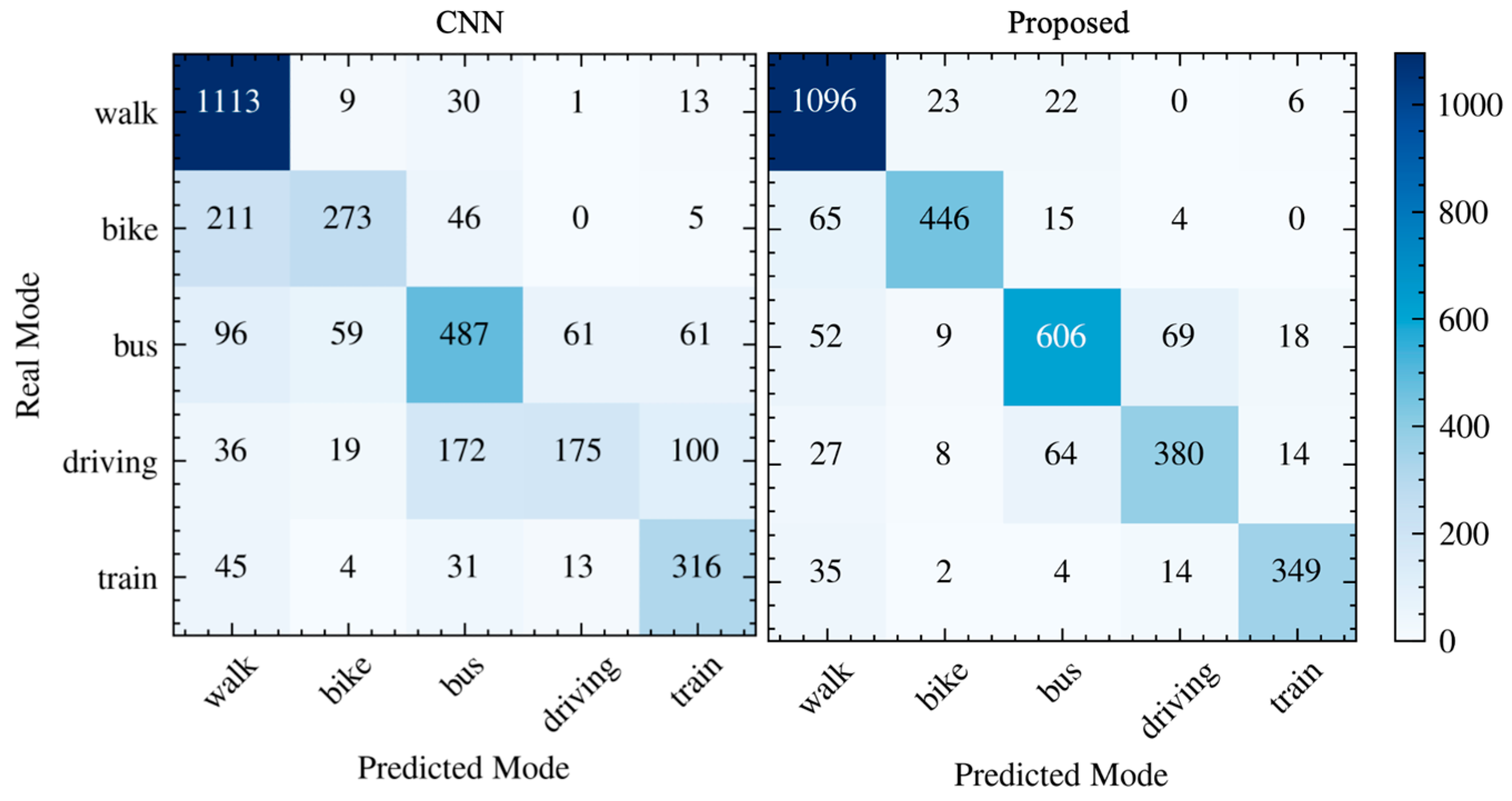
and Figure 10 demonstrate that MVCF-TMI, which utilizes multi-view contrastive (MVC) fusion, outperformed baseline approaches in accurately classifying transportation modes and minimizing confusion between different modes. The comparison in Table 8 is specifically designed to validate the effectiveness of feature-level fusion with MVC. To achieve this, we contrasted input- and feature-level fusion methods. The results showed that the proposed method, incorporating feature-level fusion with multi-view contrastive learning, more effectively captured kinematic and spatial features, capturing their complementary properties. This enhanced trajectory representation improved TMI accuracy, highlighting the advantages of MVC fusion.

The proposed method achieved an overall accuracy of 86.45%, nearly 3% higher than the best baseline. It also outperformed the baseline in classifying most modes while significantly reducing misclassifications between similar modes. For example, it provided a clearer separation between train and other modes and better distinguished between driving and bus modes than the baseline CNN model (Figure 10). This performance demonstrated that the multi-view contrastive representation learning captures more comprehensive and discriminative features.

We compared the representation distributions of our proposed method with the CNN-based input-level fusion approach using 2D-tSNE visualization. The CNN method tends to confuse representations from similar categories, such as walk vs. bike, bus vs. driving, and driving vs. train, leading to less distinct inter-class boundaries (Figure 11). In contrast, our method effectively differentiated these ambiguous categories. This result demonstrated that by preserving complementary multi-perspective information, our approach better distinguished similar trajectories with close semantics, aligning with the confusion matrix in Figure 10.

5.3.2. Travel Mode Classification Performance Comparison

Table 9. Comparison of SOTA TMI methods.

Method	Number of Samples	Accuracy
Graph-based [49]	Unknown	79.8%
One-stage PointNet [11]	Unknown	84.9%
TaaS [48]	139,480 (frames)	85.23%
MASO-MSF [6]	9488	92.25%
MVCF-TMI	16,907	86.45%

compares our method’s performance on the GeoLife dataset with recent studies from the past two years, showcasing its competitive results. Yu and Wang proposed a graph-based method to capture spatial correlations between trajectories [49], achieving 79.8% accuracy with only 20 points per trajectory. Li improved the PointNet for pointwise TMI [11], achieving 84.9% accuracy.

The TaaS approach [48] utilized a sequence-based model (RCRF) to capture temporal dependencies between motion features extracted using CNN from trajectories, achieving 85.23% accuracy on a similar subset of the downsampled GeoLife dataset. While sequence models excel at outputting reasonable travel mode label sequences, our method advanced the TMI field by presenting a novel approach that integrates spatial and kinematic views through contrastive learning.

Ma et al. introduced “MASO-MSF”, which combined multiscale spatial patterns and kinematic attributes, enhancing feature space for recognition models [6]. The accuracy difference between our method and MASO-MSF can be attributed to preprocessing variations, with our study using 16,907 samples, compared to 9488 in MASO-MSF [6]. Additionally, our multi-view architecture offers computational advantages over input-level fusion methods like MASO-MSF. Under identical GPU memory conditions (24GB), our approach accommodated larger batch sizes (up to 256) compared to input-level fusion methods (around 64), making it more practical for real-world deployment.

Although our method did not achieve the highest accuracy, it achieved comparable results while introducing an innovative trajectory feature fusion technique, contributing to the integration of multi-view trajectory features, which represents a significant advancement in TMI.

5.4. Ablation Study

We conducted an ablation study to evaluate the effectiveness of each component of the proposed framework. As outlined in Section 4.4, the framework included a contrastive learning component comprising IVCL, the view-specific classification guided (VCG) mechanism, and the weight factor $w$ to emphasize challenging samples. We performed three experiments, each omitting one component from the joint training objective, and reported the TMI results in

Table 10. Ablation study results on model objectives.

Index	Multi-View Interaction	Accuracy%	Precision%
(1)	w./o. IVCL	85.49	85.58
(2)	w./o. VCG	84.68	84.72
(3)	w./o. $w$	85.91	86.16
-	Proposed	86.45	86.49

.

In experiment 1, we removed the IVCL ${\mathcal{L}}_{\mathrm{ViewCon}}$ which aligns representations from different views, resulting in directly connected encoder outputs without view interaction. This approach led to a drop in accuracy to 85.49% and precision to 85.58%, highlighting the importance of this alignment for effectively utilizing multi-view data.

In experiment 2, we employed the fully supervised multi-view contrastive scheme from [87] to align the representations of different views before creating joint embeddings, but without the view-specific classification guidance. This phenomenon caused accuracy to decrease to 84.68%, demonstrating the value of view-specific supervision in enhancing the model’s ability to learn complementary information from various views.

In experiment 3, we did not assign any weight to in-batch samples, which resulted in a reduction in accuracy to 85.91% and precision to 86.16%. This result emphasized the role of the weight factor $w$ in improving model performance by ensuring complex samples are given proper attention, thereby enhancing the model’s ability to distinguish between similar travel modes.

5.5. Parameter Sensitivity: Influence of Parameters $\lambda and p$ on Accuracy

We investigated the impact of two key parameters on TMI accuracy: the spatial–kinematics view trade-off parameter $\lambda$ (Equation (16) and the scaling factor of multi-view contrastive loss $p$ (Equation (24). A grid search was conducted within the ranges [0, 0.3] for $p$ and [0, 3] for $\lambda$ using the GeoLife dataset. The results, shown in Figure 12, revealed that the model’s accuracy in TMI remained stable despite variations in $\lambda$ and $p$, with minor fluctuation near optimal values, when $\lambda$ was around 2 and $p$ was approximately 0.05.

5.6. Generalizability with SHL Datasets

To evaluate the model’s robustness across datasets with varying distributions and sizes, we conducted generalization experiments on both the GeoLife and SHL datasets under self-supervised and supervised paradigms. These datasets present significant differences in terms of geography (Beijing vs. southeastern UK), sampling rates (1–5 s in GeoLife vs. consistent 1 Hz in SHL), and sensor placement (varied in GeoLife vs. controlled positions at hand, torso, hips, and bag in SHL). The contrastive learning framework allowed pretraining on large, unlabeled datasets in a self-supervised manner, followed by fine-tuning on smaller labeled datasets, such as SHL. This approach outperformed direct training on small, labeled datasets. For self-supervised pretraining, an unsupervised contrastive loss was used, while supervised fine-tuning involved the proposed framework with contrastive fusion and the overall objective ${\mathcal{L}}_{Overall}$ for joint learning.

In the “No Pretrain SHL” setting (

Table 11. Generalization results on the SHL dataset.

Models	Supervision	Acc%	Acc↑%
No pretrain	Supervised	75.62 ± 1.25	-
Pretrained on GeoLife	Supervised	79.69 ± 0.0	4.07 ± 1.25
	Self-supervised	79.37 ± 1.17	3.75 ± 0.08

), the model was trained and tested directly on labeled SHL data with a 4:1 train/test split, achieving an accuracy of 75.62 ± 1.25%, which served as the baseline. The “Pretrained on GeoLife” setting included both supervised and self-supervised pretraining on the GeoLife dataset, followed by fine-tuning on SHL. In the self-supervised approach, the final training objective consisted solely of the contrastive loss, without any labeled data.

The results indicated that pretraining on the GeoLife dataset and fine-tuning on SHL led to a notable accuracy improvement of 4.07 ± 1.25%, demonstrating effective knowledge transfer between the datasets despite their geographical and data collection differences. Our image-based representation approach helps mitigate sensor position variations by focusing on trajectory patterns rather than absolute sensor readings, while the multi-view architecture effectively captures both kinematic and spatial features across different urban environments.

Additionally, the self-supervised approach using the multi-view contrastive learning framework achieved an accuracy of 79.37 ± 1.17%, reflecting a 3.75 ± 0.08% improvement. This result demonstrated the model’s strong generalization capabilities, even without labeled data during pretraining. Overall, both pretraining methods significantly enhanced classification performance on SHL, underscoring the model’s robust generalization and its potential to improve TMI using large, unlabeled trajectory datasets from diverse geographical contexts and data collection settings.

6. Conclusions and Future Work

This paper presented MVCF-TMI, a novel multi-view contrastive joint learning framework designed to address spatial–kinematic feature learning and fusion for GPS-based TMI. By integrating view-specific and multi-view contrastive learning into a unified optimization process, our method effectively learned complementary information from trajectories, enhancing TMI. The spatial–kinematic contrastive learning module improved the discriminative power of each view, yielding informative representations for final prediction. Extensive experiments demonstrated significant performance improvements over traditional machine learning methods and recent input-level fusion deep learning models. On the GeoLife dataset, the proposed method achieved 86.45% accuracy, outperforming the compared baseline methods.

Our approach offers several key advantages. First, our feature-level fusion paradigm preserves complementary information from spatial and kinematic features, improving the representation of both spatial patterns and kinematic characteristics. Second, the contrastive learning mechanism enhances the model’s ability to distinguish transportation modes with similar spatial patterns but different velocity profiles, and conversely. Additionally, our method showed strong generalizability, with accuracy improvements of up to 4.07% across various datasets, proving its robustness in different settings. The framework also flexibly supports both supervised and self-supervised pretraining, enabling effective training even with limited labeled data. Finally, our method significantly reduced computational requirements, using GPU memory more efficiently and accommodating larger batch sizes compared to input-level fusion methods. These benefits make MVCF-TMI well-suited for real-world TMI applications, where performance, adaptability, and efficiency are critical.

Several limitations still remain to be further explored. First, the contrastive loss relies on supervised signals for view-specific classification, requiring labeled trajectory data. Second, the current framework focused solely on TMI, whereas real-world trajectory analysis involves tasks, such as trajectory similarity and destination prediction, where the learned representations may not generalize as effectively. Third, interpolation techniques could be explored to reduce sparsity in image representations, especially for irregularly sampled trajectories. Additionally, validating the effectiveness of our method on newer datasets (e.g., the TMD dataset [88]) would provide a more comprehensive assessment of its generalizability across diverse scenarios.

Moreover, our current framework primarily relies on GPS trajectory data, while smartphones offer rich sensor data (e.g., accelerometers, gyroscopes, and magnetometers) that could further enhance classification accuracy. Future work could explore a fusion that integrates these additional data sources with our current approach. Furthermore, since GPS trajectories inherently exhibit temporal dependencies, incorporating sequence models (e.g., LSTMs or Transformers) could potentially reduce the need for extensive feature engineering while automatically capturing complex temporal patterns in movement data.

Another promising direction is to represent trajectory segments as video sequences, where consecutive subsegments act as frames. This would allow the use of video classification techniques to capture both spatial and temporal patterns. Each trajectory could be divided into overlapping time windows, with frames displaying spatial points and features like speed and acceleration. This approach could be effective for transportation modes with distinct temporal-spatial signatures, such as buses or trains, and handle varying trajectory durations without the need for fixed-length sequence models. Additionally, integrating GIS data, weather, and environmental context could help capture broader contextual factors influencing travel patterns, further enhancing model robustness.