Abstract
Topological relations form the backbone of qualitative spatial reasoning and, as such, play a paramount role in geographic information systems. Three decades of research have provided a proliferation of sets of qualitative topological relations in both continuous and discretized spaces, but only in continuous spaces has the concept of organizing these relations into a larger framework (called a conceptual neighborhood graph) been considered. Previous work leveraged matrix differences to derive the anisotropic scaling neighborhood for these relations. In this paper, a simulation protocol is used to derive conceptual neighborhood graphs of qualitative topological relations in for the operations of translation and isotropic scaling. It is further shown that, when aggregating raster relations into their continuous counterparts and collapsing neighborhood connections within these groups, the familiar conceptual neighborhood structures for continuous regions appear.
1. Introduction
Egenhofer and Mark [1] made a provocative statement in their seminal work of Naïve Geography: topology matters and metric refines. This statement comes directly from the notion that many human decisions about space are either fully or partially sufficient when considering the basic construct of a spatial preposition. While there are lots of spatial prepositions in a language context [2], not all spatial prepositions are grammatically prepositions. Terms like surrounds communicate spatial information about the topological relation between two objects, yet the word itself is not syntactically a preposition in established grammar [3,4]. At any rate, terms that function linguistically as prepositions do so because they greatly reflect our cognitive processing [5,6,7,8]. This concept is directly mirrored in conceptual neighborhood graphs [9] in which researchers have shown that spatial prepositions map convexly onto these structures [10]. An example of this phenomenon would be the term along, which describes instances from any number of primitive topological relations, but those topological relations themselves are in predictable and nearby positions within a conceptual neighborhood graph.
The world is currently in an information age, one that is exploding daily. Query languages leverage spatial concepts [11,12], but they do so atomically and in vector spaces, despite the occurrence of baseline raster data available in the world and the fundamental presence of uncertainty or vagueness in human reasoning. Conceptual neighborhood graphs have been well studied [13,14,15,16,17], but these approaches have not found their way into computational tools that are used in practical applications [18]. This oversight hinders crucial next steps in geospatial knowledge discovery. Since spatial concepts are critical to language [19] and our language controversially may influence our world view [20], generative artificial intelligence relies on being able to fully process spatial data to meaningful speech and/or text through geo-foundation models [21], just as an effective spatial query relies on translating human language to computational data structures [11]. It is, therefore, necessary to leverage conceptual neighborhood graphs to perform various tasks such as detecting events, contextualizing prepositional definitions based on the use case, and filling in gaps of incomplete data within spatial data streams.
While conceptual neighborhood graphs have been well studied, their study has been largely limited to continuous spaces, supporting vector-based tools and implementations. To date, discretized region–region neighborhoods have been exploited simply by using the matrix difference method [22,23,24]. This method only works for the transformation of anisotropic scaling. To fully realize the other spatial operations that generate neighborhoods in discretized spaces, work needs to be conducted. This paper fills that gap.
While vector data are widely used in GISs, raster-based representations are still critical for applications like remote sensing, environmental modeling, and spatial simulations. Many geographic datasets, particularly from satellite imagery and sensor networks, are inherently raster-based. By extending conceptual neighborhood graphs to discretized relation sets, this work provides a framework for analyzing topological transitions in pixel-based spatial processes, ensuring broader applicability beyond the traditional vector-based GIS. Furthermore, developing direct raster functionality reduces levels of data transformation, keeping us closer to the root source of the data itself, a core data quality issue.
In this paper, the region–region relations in [22] are exposed to a simulation protocol to establish conceptual neighborhood graphs for both translation and isotropic scaling. Leveraging duality [25], these neighborhoods are then transferred into their digital spherical space () counterparts [24]. The hyperraster representation of discretized regions [26] is then leveraged to provide a proof of concept to show that conceptual neighborhood graph edges in discretized spaces appropriately maintain their corresponding connections in well-studied continuous spaces [16].
The remainder of this paper is structured as follows. Section 2 details the set of qualitative topological relations considered in this work. Section 3 details conceptual neighborhood graphs. Section 4 defines the simulation protocol and methodology employed upon the output data. Section 5 presents the results of the data processing. Section 6 applies the hyperraster as a transformation to explore the structural integrity of the discretized neighborhood graphs with respect to their continuous counterparts. Section 7 considers a use case for the outcomes. Section 8 provides conclusions and calls for future study in this area.
2. Region–Region Relations in Continuous and Discretized Spaces
To conduct qualitative topological spatial reasoning, it is imperative to establish a vocabulary. Since this paper leverages both continuous (vector) and discretized (raster) relations, we introduce both in this section.
Linguistically, qualitative spatial relations of any form represent functional prepositions [2,27]. While these terms differ in their respective languages and might be represented in various parts of the overall grammatical syntax, they represent the expression of our cognitive processes. Our formal models of topological spatial relations, thus, represent attempts to encode these cognitive processes into machines through rigorous mathematical approaches, be they by topological means [10,11,28,29,30], mereotopological means [31,32], graph theoretical means [3,33], or by means of metric refinement [34,35,36]. In general, these processes anchor the Egenhofer–Cohn hypothesis of the salience of topological relativity, namely that topological properties fundamentally drive human decision making [37]. This becomes foundational for understanding human-sourced data that become part of generative AI scenarios and also for providing the tools for humans to meaningfully query spatial data on their own.
Spatial data for qualitative topological reasoning can be seen as originating in a combination of two forms: (a) vectorized or rasterized and, simultaneously, (b) localized or globalized. Each dataset represents a combination of both (a) and (b). The various combinations of these two properties lead to mathematical models formalized in one of four embedding spaces:
- Vectorized and localized:
- Vectorized and globalized:
- Rasterized and localized:
- Rasterized and globalized:
Conceptually, within spatial data, we can view relations from the localized spaces as a restricted set of relations from the corresponding globalized spaces. Similarly, we can view rasterized and vectorized views of the same scope of space as different levels of granularity in how we represent those data, each with fundamentally different mathematical properties to exploit.
While many formalisms exist for these spatial concepts, this paper focuses on the 9-intersection family of qualitative topological reasoning [28,29,30]. This family of models partitions an embedding space through the existence of two objects and uses topological definitions within the structure of those objects to categorize the partitions. The most basic form of this approach is the 9-intersection model [28]. This model classifies three jointly exhaustive and pairwise disjoint portions of the embedding space with respect to a set: the interior, boundary, and exterior. Depending on the type of object, this approach may leverage point-set topological concepts (such as in codimension 0 embeddings) [29] or algebraic topological concepts (such as in codimension > 0 embeddings) [38]. By applying this partitioning mechanism to multiple objects, we can then consider binary (or beyond) qualitative topological relations. Figure 1 shows the possible outcomes of the 9-intersection model on simple regions in , the most iconic set of relations derived via this methodology.
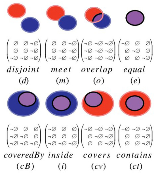
Figure 1.
Eight qualitative topological relations between simple regions in [28]. The red object represents the first object; the blue object represents the second object; the purple object represents mutual occurrence of the red and blue objects. The 9-intersection matrix associated with each relation is provided. For more details on the 9-intersection, please consult [28].
Simple regions, however, create a dilemma: for all three topological components of an object, that component will be connected. When applying these concepts to other types of objects, that might not be the case. Kurata [30] thus developed the 9+-intersection, an approach considering separated portions of topological components as having their own symbolic place in the formal representation. This approach increases the complexity of the representation but, thus, provides more expressive power, a boon for reasoning systems that need to exhibit more nuance in applications.
Borrowing loosely from Kurata’s approach, the expression of discretized topological relations in and can leverage the proximity of distinct partitions to boundary pixels to provide more refined semantics to certain 9-intersection relations. These relations are known as the dTouch relations—relations that help to refine otherwise indistinguishable topological relations in rasterized spaces that would have a corresponding difference in vector spaces [22,24]. The set of qualitative topological relations in is shown in Figure 2 and Figure 3.
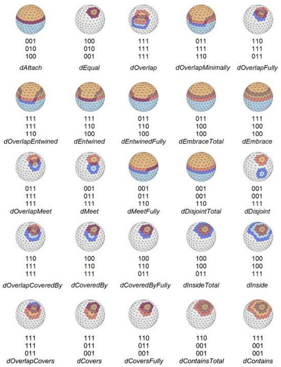
Figure 2.
9-intersection qualitative topological relations on the digital sphere [24].
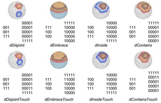
Figure 3.
The touch relations distinguished from their vanilla counterparts from Figure 2 [24].
In both cases, the sets of relations output by the 9-intersection family are jointly exhaustive and pairwise disjoint, meaning that, for any configuration, there exists a single 9-intersection family symbol specific to it. These relations in Figure 1, Figure 2 and Figure 3 form the foundation for the remainder of this paper.
3. Conceptual Neighborhood Graphs
Sets of topological relations represent the foundations for qualitative spatial reasoning tools within GIS, but they themselves do not form the totality of topological spatial knowledge. We live in a changing world, and that dynamism gives rise to an entirely different concept that is critical to knowledge within spatial reasoning: relational ordering and/or sequencing. While humans intuitively know that there is a fundamental ordering between terms that they use daily (such as prepositions), artificial intelligence (and other computational tools) has to either learn that or be given the concept explicitly. Conceptual neighborhood graphs represent that ordering/sequencing [9]. Conceptual neighborhood graphs partially order sets of relations based on allowable deformations. While Freksa’s work [9] focuses on temporal semi-intervals [39], Egenhofer and Al-Taha [13] conducted a similar study on simple regions. Their work derived three conceptual neighborhood graphs for homeomorphic deformations, representing anisotropic scaling (non-homogeneous growth/decline), translation (movement), and isotropic scaling (homogenous growth/decline). These conceptual neighborhood graphs (when applied to continuous spherical topological relations) are shown in Figure 4.
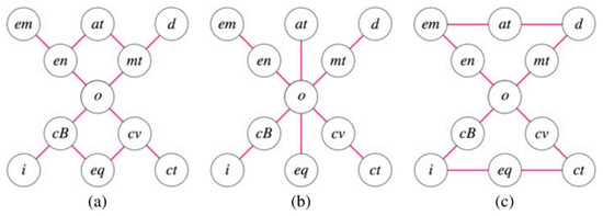
Figure 4.
Conceptual neighborhood graphs of (a) anisotropic scaling, (b) translation, and (c) isotropic scaling [15].
Conceptual neighborhood graphs have also been applied to a different class of transformations: non-homeomorphic deformations [40]. Non-homeomorphic deformations involve changing the number of distinct topological subcomponents of objects, such as holes or separations. These concepts were organized into a conceptual neighborhood graph [17], but that work is beyond the scope of this paper.
Common to all conceptual neighborhood graph studies in the literature is a process by which candidate relations are identified as conceptual neighbors. Many studies achieve this in a variety of ways:
- Freksa [9] approached the problem through considering the ordering of the boundary points of the semi-intervals within a space based on the corresponding mathematical changes exhibited by the objects.
- Egenhofer and Al-Taha [13] approached the problem through studying deformational paths based on the various strategies, starting at all possible configurations and creating a union of the various deformation paths.
- Researchers who defined relations alongside neighborhood graphs (e.g., [15,17,22,23,24,38]) approached the problem by consulting the smallest matrix differences, but this approach only yields the anisotropic scaling conceptual neighborhood graph.
While continuous spaces such as those explored by Freksa [9] and Egenhofer and Al-Taha [13] operate under an assumption of mathematical density, discretized spaces are not dense. As such, a different approach might be taken whereby a computer can assist in a simulation process, as opposed to the thought experiments of Egenhofer and Al-Taha [13]. The next section defines this process as employed in this study.
4. Simulation Methodology for Establishing Conceptual Neighborhood Graphs
While continuous spaces have infinitely many versions of a single transformation, discretized spaces have a much more finite range of possibilities. Translation for example is achieved by shifting an object one pixel at a time; isotropic scaling is performed by uniformly adding/subtracting one pixel at a time in all directions. Whereas Freksa [9] and Egenhofer and Al-Taha [13] had to conceptually conduct their experiments, discretized spaces afford the opportunity to simulate the results rigorously.
To study the relevant deformations, a simulation protocol was developed in Python 3.8. The smallest objects considered were 4 pixels by 4 pixels (consistent with the definition of objects from [22,24]), and the largest objects considered were 10 pixels by 10 pixels. The embedding space was encoded as a 30-pixel by 30-pixel grid to allow objects to have the relation dDisjoint or dDisjointTouch to each other in any direction so that all the relations possible could be represented. Each successive iteration kept one object’s top-left corner anchored at position (11,11) in the grid, while the other moved right-to-left across the grid. At each step, the topological relation was computed. When the grid was exhausted, the object was moved back to the right-hand side of the grid and moved one pixel vertically while the process continued. This process continued until the entire space of positions for the moving object had been exhausted. The size of the moving object was then modified by one pixel, and the process repeated. Once all combinations (4,10) × (4,10) were completed, the central object was modified similarly, and the process repeated. A pseudocode of this simulation is shown in Figure 5, and an example of the stored data is shown in Figure 6.
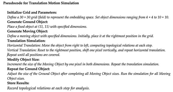
Figure 5.
Pseudocode for the simulation protocol [18].
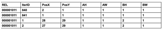
Figure 6.
Example rows of the collected data [18].
With the simulated data in tow, this paper will now proceed to describe the process by which the data can be connected using SQL to appropriately reflect the two missing neighborhood graph structures.
5. Processing the Simulations into Conceptual Neighborhood Graphs
To develop conceptual neighborhood graphs from the simulations, it was determined mathematically what a particular deformation should look like within the collected dataset. This determination motivates the eventual SQL query to extract the edges of the neighborhood graphs.
5.1. Translation Conceptual Neighborhood Graph
Translation (Figure 7) has a straightforward signature. Under translation, the objects themselves do not change in their size; they just move. As such, the sequence of changes need only consider that one of the coordinates in the grid is offset by precisely one pixel, while the others are the same. Furthermore, the sizes of the two objects must remain the same. An edge of the conceptual neighborhood graph is formed when the relations under such conditions differ. This information structures an SQL query that directly isolates the relevant records to be joined together, as shown in Figure 8. Figure 9 presents the connectivity information in graphical form.
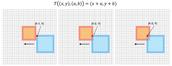
Figure 7.
Mathematical definition of translation for (a,b) = (−1,0), (−2,0), and (−3,0) [18].
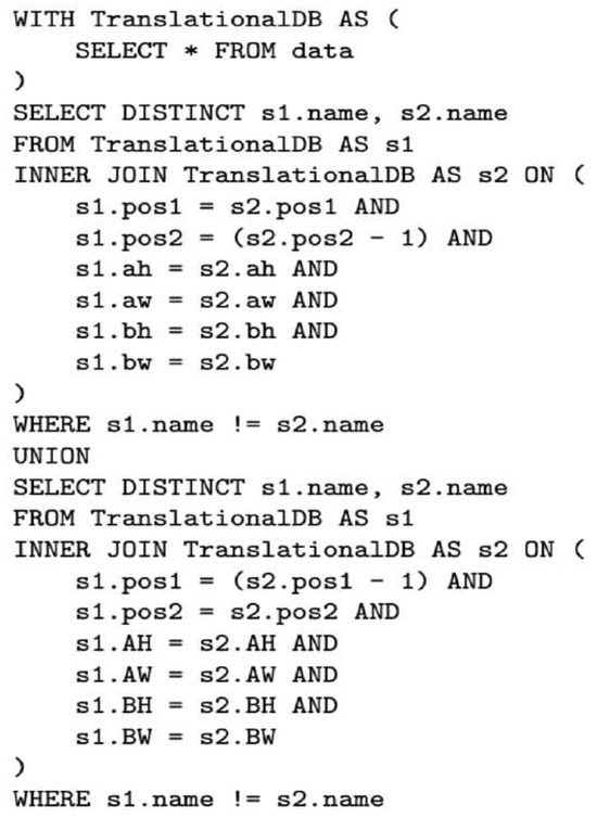
Figure 8.
SQL query exploiting the definition of translation within the dataset [18].
Figure 9.
Resulting graph of the connected relations in an unfiltered case (left) and pruned case (right). The pruned case removes instances that are only connected in specific instances but otherwise are not connected, consistent with prior methodologies of conceptual neighborhood graph research [18].
Figure 9 represents something very specific: the existence of objects that can make the change from one relation to another at least one time juxtaposed with those that can always occur when the relation is relevant to the pair of objects. Both Freksa [9] and Egenhofer and Al-Taha [13] correct against this occurrence, because, ultimately, it is important to recognize the overall patterns that consistently appear rather than those that can only appear under very specific restrictive conditions. This is critical for information systems—the last thing practically desirable in an information system is a spurious conclusion motivated by a special case. A similar occurrence of such a phenomenon is the direct linkage between overlap and equal (see Figure 1) that could be facilitated by specific configurations of objects [13].
To correct for this in the simulation approach, an association rules approach [41] was employed as demonstrated in Figure 10, Figure 11 and Figure 12. Figure 10 displays the relations dDisjoint/dDisjointTouch and dOverlapFully, both of which are never conceptual neighbors at any size. Figure 11 displays the relations dOverlapMinimally and dOverlapFully, relations that are conceptual neighbors under very strict size conditions but not otherwise. Figure 12 displays the relations dDisjoint/dDisjointTouch and dMeet, relations that are always conceptual neighbors when mutually available. Relation pairs with patterns like that in Figure 12 become the edges of interest for the salient conceptual neighborhood graph for translation. It is of course potentially relevant in context to care about relations that are neighbors in a pattern similar to that in Figure 11 and simultaneously to those with patterns similar to Figure 12.
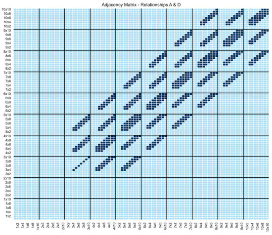
Figure 10.
Presence of mutually available relations (dark blue) and detected neighboring relations (yellow) for dDisjoint/dDisjointTouch and dOverlapFully [18]. No yellow cells are present, signifying that these relations are never conceptual neighbors.
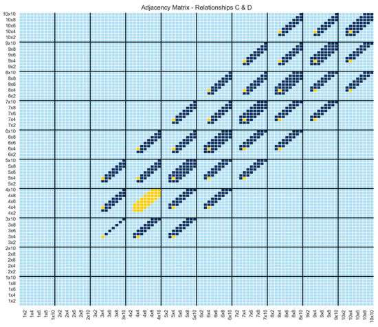
Figure 11.
Presence of mutually available relations (dark blue) and detected neighboring relations (yellow) for dOverlapMinimally and dOverlapFully [18].
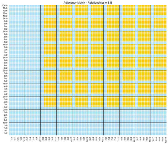
Figure 12.
Presence of mutually available relations (dark blue) and detected neighboring relations (yellow) for dDisjoint/dDisjointTouch and dMeet [18]. No dark blue cells are present, signifying that these relations are always conceptual neighbors when mutually available.
By considering all edges in Figure 9 that correspond to the pattern (all yellow) from Figure 12, the conceptual neighborhood graph can be successfully pruned to that shown in Figure 13 and Figure 14. Figure 13 consists of the relations available in the digital plane. Figure 14 is constructed by applying the dual transformations [25] to the spherical relations.
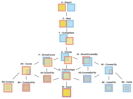
Figure 13.
Resulting translation conceptual neighborhood graph [18].
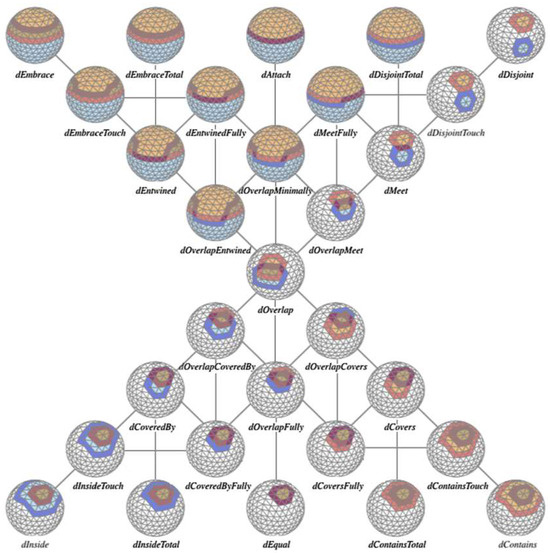
Figure 14.
Spherical conceptual neighborhood graph for translation [18].
The output of this process represents a striking structural similarity to what we see in Figure 4b. The relations show a vertical edge structure persisting throughout the conceptual neighborhood graph. This same sort of pattern adherence appears between the anisotropic scaling conceptual neighborhood graphs established in the literature with diagonal legs [13,15,22,23,24]. We will discuss this outcome more in the Conclusions and Future Work Section as a different feature than what we might hypothesize has arisen, maintaining some (but not all) diagonal connections.
5.2. Isotropic Scaling Conceptual Neighborhood Graph
Following a similar procedure to the translation conceptual neighborhood graph, the first step is to isolate exactly what isotropic scaling looks like in the dataset. In this case, the position of the top-left corner dictates the change. If the top-left corner has (x + 1,y + 1) and the size of the object is −2 in both dimensions, this is the appropriate symbol for the object isotropically shrinking; if it is (x − 1,y − 1) and the size of the object is +2 in both dimensions, this is the appropriate symbol for the object isotropically growing. Figure 15 shows the concept of growing by 1 unit in all directions.
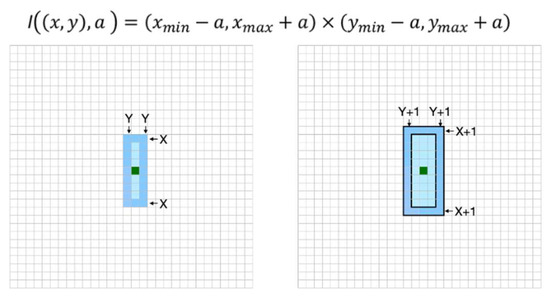
Figure 15.
Isotropic growth of an object by one pixel in all directions [18].
The change described in Figure 15 can be systematically isolated as an SQL query on the dataset as shown in Figure 16.
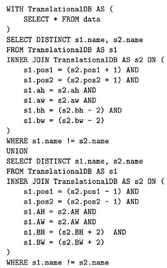
Figure 16.
SQL query implementing isotropic scaling upon the simulated data.
Unlike with the translational query, the isotropic query holds no spurious connections. As such, the conceptual neighborhood graphs for isotropic scaling are presented in Figure 17 and Figure 18. As in Figure 13 and Figure 14, Figure 17 is transformed into Figure 18 through the duality operation [26].
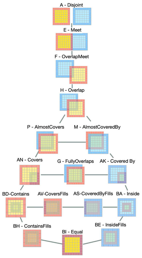
Figure 17.
Isotropic scaling conceptual neighborhood graph for planar discretized regions [18].
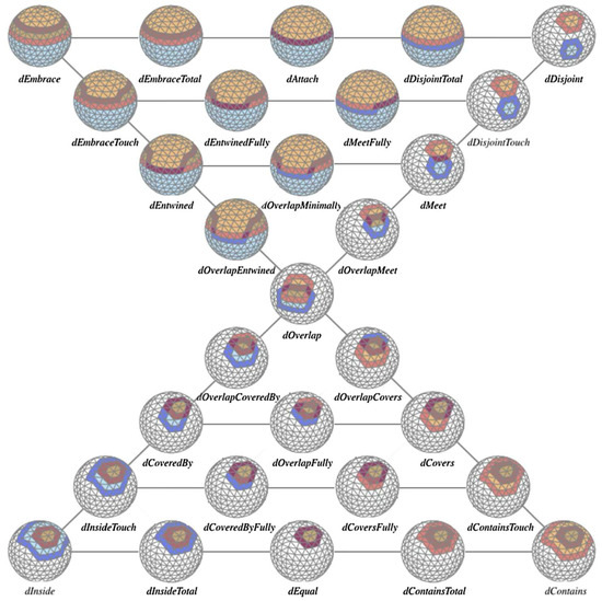
Figure 18.
Isotropic scaling conceptual neighborhood graph applied to the spherical relations [18].
6. Litmus Test for Conceptual Neighborhoods from Simulation: The Hyperraster
Winter [26] proposed a data structure for rasterized regions that effectively in sum made them consistent with vectorized regions from the perspective of the 9-intersection called the hyperraster. This data structure treats the boundary of an object as the gap between its outermost pixels and the pixels that do not belong to it, retaining the structure of the boundary of a polygonal object in . This structure effectively turns the 19/29 rasterized region relations [22,24] into the 8/11 vectorized region relations [15,29]. This approach is the conceptual backbone for modern techniques that resolve rasterized data sources to vector objects.
To evaluate the simulation approach in this work, the hyperraster definition is applied to the relations, and the corresponding conceptual neighborhood graphs are aggregated in Figure 19 and Figure 20.
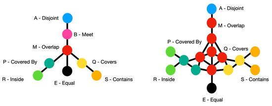
Figure 19.
Translation conceptual neighborhood graphs categorized by hyperraster relation [18].
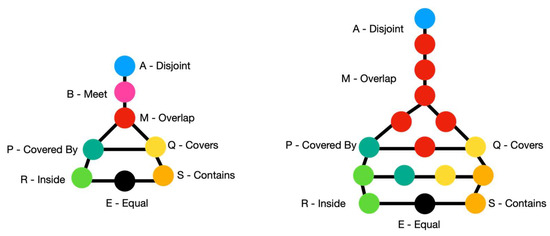
Figure 20.
Isotropic scaling conceptual neighborhood graphs categorized by hyperraster relation [18].
The differences in Figure 19 and Figure 20 are only in the classification of meet. Because dDisjointTouch was not separated from dDisjoint in the simulations, the meet relation does not appear. However, given the nature of both translation and isotropic scaling, the connectivity between dDisjoint and dMeet must be through dDisjointTouch as the growth of an object occupies the outer margin when at first it did not, thus implying dDisjoint—dDisjointTouch—dMeet, and, similarly, the movement of an object implies the same transference. As such, any of the dTouch relations fit firmly between their corresponding dual counterparts in the conceptual neighborhood graphs, as demonstrated in the expansions to the spherical relations in Figure 14 and Figure 18. This result serves as a critical litmus test—when converted to vectorized regions, the exact neighbors that exist in the conceptual neighborhood graphs are the only neighbors that appear in the conceptual neighborhoods of these discretized relations. Had the simulation approach failed, these conceptual structures would not have been able to be merged appropriately.
7. Utility of the Outcome: Processing Pixelated Maps in Various Circumstances
Conceptual neighborhood graphs have heretofore been underutilized concepts in the informatics realm. One particular reason for this corresponds to the architecture of spatial data as just that: spatial data. The temporal dimension of spatial data is often minimally analyzed within the context of geographic information systems. With changes in data architecture [42,43], a set of use cases emerges for conceptual neighborhood graphs.
While cadastral records are not traditionally found in raster formats, legacy records brought directly into an analysis in image format or vectorized cadastral records super-imposed on an orthophoto represent an opportunity to see the importance of the conceptual neighborhood graph architecture with respect to a spatial information system. It is important to consider that objects that may originate from rasterized sources have an additional layer of uncertainty as mentioned in the introduction, and the consequence of that uncertainty has a specific impact on the information system, specifically that a specified topological relation that would motivate a spatial query may not be all inclusive of the phenomenon in question from the viewpoint of the rasterized relation. There are two critical examples of this. The first is the search for trees that encroach upon property lines, whereas the second is the search for buildings or driveways that approach property lines. Humans are rightly prone to vocabulary suggestive of the physical world and its continuous topological relations [5,6,7,8,37]. As such, a human might choose to query such a database system using overlap in the first case and meet in the second case. If the stored data considering the cadastral records are discretized, these terms occupy specific relations in the conceptual neighborhood graph. Based on such concepts as resolution, position, or sheer lack of terminology, other conceptual neighbors from Figure 13, Figure 14, Figure 17 and Figure 18 are likely to satisfy the wishes of the user based on equivalencies from Figure 19 and Figure 20, and thus should be a logical included option in topological query systems. Similarly, a user should be able to fine-tune which conceptual neighbors are relevant to the appropriate application.
Conceptual neighborhood graphs allow for the realization of temporal events within spatial data. Rather than considering one layer of spatial data, we could consider multiple layers of spatial data and observe the changes between the topological relations of objects. This scenario creates two use cases as well. The first use case is the discovery of an event such as becoming adjacent, reflecting the change from dDisjoint to dDisjointTouch or dDisjointTouch to dMeet (as determined by the desires of the user). Becoming adjacent differs from adjacent insofar as there is a communicated desiderata that the event does not start in the final configuration but rather progresses to that configuration from the outside. This type of question is only answered through information in the various conceptual neighborhood graphs. The second use case accounted for, in this scenario, is the determination that a state change is missing within the data due to combinations of spatial and temporal resolution. If consecutive time stamps represent non-conceptual neighbors, a missing relevant state can be discovered, thus increasing the intrinsic data quality of our data by increasing its completeness. Such an application is critical to generative artificial intelligence that attempts to leverage image data to glean insights.
To be clear, these particular use cases are not unique to rasterized objects; conceptual neighborhood graphs are simply not leveraged in software applications where they otherwise should be. Rasterized objects only further demonstrate this problem because they possess a much richer vocabulary.
8. Conclusions and Future Work
In this paper, the conceptual neighborhood graphs of discretized topological relations have been determined using a simulation protocol and corresponding queries to tease out persistent conceptual neighbors from the data. This approach extends the conceptual neighborhood graphs available to discretized regions in both and to be consistent with those available for and [13,15].
The translation neighborhood graph (Figure 13 and Figure 14) shows a pattern that is slightly different than what we might have expected when considering the corresponding continuous neighborhood (Figure 4b). While this might at first suggest a problem with the simulation procedure, what is occurring is the fundamental lack of relation diversity in continuous spaces that is filled in within discretized spaces. The lower part of the continuous neighborhood does not have an appropriate number of relations within it to show the patterns depicted in Figure 13 and Figure 14. Under the aggregation test, we observed the continued orphaning of the inside/coveredBy and contains/covers relations with respect to equal, a critical evaluation criterion. In other words, equal is only accessible from an overlap condition, and a very specific one at that (namely dOverlapFully). We similarly observed a consistent conceptual neighborhood graph structure for isotropic scaling, in which the expectation from the continuous spaces was directly mirrored in discretized spaces without any surprises.
The world of big data necessitates that analysis procedures can be applied to both vector data and raster data, reflecting notions of interoperability stemming from the fundamental variety of data sources in our world. The work undergone here paves the way for software libraries that can process spatio-temporal queries that reflect the dynamically changing states of objects in various embeddings. To meet this demand, there is a critical need for the revisement of infrastructure in spatial databases to incorporate queries that target the change in object relations directly. Furthermore, modern spatial programming libraries need to implement raster protocols for working with the 9-intersection to make this aspiration a reality. To achieve these means, we need to embark on an architecture of space–time cubes for rasterized data [42] and temporal layering for continuous data [43].
There is more work to be undertaken in the pursuit of these conceptual neighborhood graphs. The base level relations considered in this paper have been further extended to line-up directly with the regions identified by the hyperraster approach [44].
These relations have a corresponding signature in the hyperraster, and, thus, the results in Figure 19 and Figure 20 provide implicit bounds for where these relations should sit schematically. More work needs to be undertaken to adequately place these relations within a larger framework. These relations themselves are special cases within the discretized relations because their boundaries and interiors violate basic properties of the digital Jordan curve [44,45]. This emphasizes the need for a deeper exploration of how these discretized relations interact with broader topological principles to refine their placement in a generalized model.
Future work may also extend conceptual neighborhood graphs to incorporate qualitative distance concepts like near and far. One approach is graph-based topological clustering, in which near corresponds to a single transition (e.g., disjoint → meet) and far to multiple transitions. These extensions would enhance qualitative spatial reasoning within conceptual neighborhood graph theory without relying on explicit metrics.
Author Contributions
Conceptualization, Matthew Paul Dube; methodology, Matthew Paul Dube; software, Brendan Patrick Hall; validation, Brendan Patrick Hall and Matthew Paul Dube; formal analysis, Brendan Patrick Hall and Matthew Paul Dube; investigation, Matthew Paul Dube; resources, Brendan Patrick Hall; data curation, Brendan Patrick Hall; writing—original draft preparation, Matthew Paul Dube; writing—review and editing, Brendan Patrick Hall and Matthew Paul Dube; visualization, Brendan Patrick Hall; supervision, Matthew Paul Dube; project administration, Matthew Paul Dube; funding acquisition, Matthew Paul Dube. All authors have read and agreed to the published version of the manuscript.
Funding
This research was funded by the National Science Foundation, grant number 2019470. The APC was waived by MDPI.
Data Availability Statement
All the data and code associated with this project can be found at https://github.com/brendanphall/BrendanHall_Research/tree/main/2024_CNG_R2 (accessed 28 March 2025).
Acknowledgments
The authors gratefully acknowledge feedback and guidance from Max Egenhofer, Kate Beard, and Nimesha Ranasinghe. The authors also gratefully acknowledge grant administration support/reporting from Brian McGill and Leo Edminston-Cyr.
Conflicts of Interest
Author Brendan P. Hall was employed by the James W. Sewall Company. The remaining authors declare that the research was conducted in the absence of any commercial or financial relationships that could be construed as a potential conflict of interest.
References
- Egenhofer, M.; Mark, D. Naïve geography. In Proceedings of the International Conference on Spatial Information Theory, Semmering, Austria, 21–23 September 1995; Frank, A., Kuhn, W., Eds.; Springer: Berlin, Germany, 1995; pp. 1–15. [Google Scholar]
- Landau, B.; Jackendoff, R. Whence and whither in spatial language and spatial cognition? Behav. Brain Sci. 1993, 16, 255–265. [Google Scholar] [CrossRef]
- Dube, M.; Egenhofer, M. Surrounds in partitions. In Proceedings of the 22nd ACM SIGSPATIAL International Conference on Advances in Geographic Information Systems, Dallas, TX, USA, 4–7 November 2014; Huang, Y., Schneider, M., Gertz, M., Krumm, J., Sankaranarayanan, J., Eds.; Association for Computing Machinery: Washington, DC, USA, 2014; pp. 233–242. [Google Scholar]
- Worboys, M.; Duckham, M. Qualitative-geometric surrounds relations between disjoint regions. Int. J. Geogr. Inf. Sci. 2021, 35, 1032–1063. [Google Scholar] [CrossRef]
- Tyler, A.; Evans, V. Applying cognitive linguistics to pedagogical grammar: The case of over. Cogn. Linguist. Second. Lang. Acquis. Foreign Lang. Teach. 2004, 1, 257–280. [Google Scholar]
- Aajami, R. A cognitive linguistic study of the English preposition ‘in’. J. Coll. Educ. Women 2019, 30, 37–49. [Google Scholar] [CrossRef]
- Aajami, R. A cognitive linguistic study of the English prepositions ‘above’, ‘on’, and ‘over’. J. Lang. Linguist. Stud. 2022, 18, 1. [Google Scholar]
- Yue, F.; Cao, S.; Huang, J. The semantic analysis of the preposition through from the perspective of cognitive linguistics. Theory Pract. Lang. Stud. 2022, 12, 400–406. [Google Scholar] [CrossRef]
- Freksa, C. Temporal reasoning based on semi-intervals. Artif. Intell. 1992, 54, 199–227. [Google Scholar] [CrossRef]
- Dube, M.; Egenhofer, M. An ordering of convex topological relations. In Proceedings of the Geographic Information Science: 7th International Conference, Columbus, OH, USA, 18–21 September 2012; Xiao, N., Kwan, M., Goodchild, M., Shekhar, S., Eds.; Springer: Berlin, Germany, 2012; pp. 72–86. [Google Scholar]
- Clementini, E.; Sharma, J.; Egenhofer, M. Modelling topological spatial relations: Strategies for query processing. Comput. Graph. 1994, 18, 815–822. [Google Scholar] [CrossRef]
- Egenhofer, M. SpatialSQL: A query and presentation language. IEEE Trans. Knowl. Data Eng. 1994, 6, 86–95. [Google Scholar] [CrossRef]
- Egenhofer, M.; Al-Taha, K. Reasoning about gradual changes of topological relationships. In Theories and Methods of Spatio-Temporal Reasoning in Geographic Space: International Conference GIS—From Space to Territory; Frank, A., Campari, I., Formentini, U., Eds.; Springer: Berlin, Germany, 1992; pp. 196–219. [Google Scholar]
- Cohn, A.; Bennett, B.; Gooday, J.; Gotts, N. Representing and reasoning with qualitative spatial relations about regions. In Spatial and Temporal Reasoning; Stock, O., Ed.; Springer: Berlin, Germany, 1997; pp. 97–134. [Google Scholar]
- Egenhofer, M. Spherical topological relations. J. Data Semant. III 2005, 1, 25–49. [Google Scholar]
- Egenhofer, M. The family of conceptual neighborhood graphs for region-region relations. In Proceedings of the Geographic Information Science: 6th International Conference, Zurich, Switzerland, 14–17 September 2010; Fabrikant, S., Reichenbacher, T., van Krevald, M., Schlieder, C., Eds.; Springer: Berling, Germany, 2010; pp. 42–55. [Google Scholar]
- Dube, M. Beyond homeomorphic deformations: Neighborhoods of topological changes. In Advancing Geographic Information Science: The Past and Next Twenty Years; Onsrud, H., Kuhn, W., Eds.; GSDI Press: Needham, MA, USA, 2016; pp. 137–151. [Google Scholar]
- Hall, B. Identification of Conceptual Neighborhoods and Topological Relations in . Master’s Thesis, University of Maine, Orono, ME, USA, 2024. [Google Scholar]
- Freundschuh, S.; Sharma, M. Spatial image schemata, locative terms, and geographic spaces in children’s narrative: Fostering spatial skills in children. Cartographica 1995, 32, 38–49. [Google Scholar] [CrossRef]
- Regier, T.; Xu, Y. The Sapir-Whorf hypothesis and inference under uncertainty. Wiley Interdiscip. Rev. Cogn. Sci. 2017, 8, 1440. [Google Scholar] [CrossRef] [PubMed]
- Xie, Y.; Wang, Z.; Mai, G.; Li, Y.; Jia, X.; Gao, S.; Wang, S. Geo-foundation models: Reality, gaps, and opportunities. In Proceedings of the 31st ACM International Conference on Advances in Geographic Information Systems, Hamburg, Germany, 13–16 November 2023; Damiani, M., Renz, M., Eldawy, A., Kroger, P., Nascimento, M., Eds.; ACM Press: Washington, DC, USA, 2023; pp. 1–4. [Google Scholar]
- Egenhofer, M.; Sharma, J. Topological relations between regions in and . In International Symposium on Spatial Databases; Abel, D., Ooi, B., Eds.; Springer: Berlin, Germany, 1993; pp. 316–336. [Google Scholar]
- Dube, M. An embedding Graph for 9-Intersection Topological Spatial Relations. Master’s Thesis, University of Maine, Orono, ME, USA, 2009. [Google Scholar]
- Dube, M.; Egenhofer, M. Binary relations on the digital sphere. Int. J. Approx. Reason. 2020, 116, 62–84. [Google Scholar]
- Dunstch, I. A tutorial on relation algebras and their application in spatial reasoning. In Proceedings of the International Conference on Spatial Information Theory, Stade, Germany, 25 August 1999. [Google Scholar]
- Winter, S. Topological relations between discrete regions. In International Symposium on Spatial Databases; Egenhofer, M., Herring, J., Eds.; Springer: Berlin, Germany, 1995; pp. 310–327. [Google Scholar]
- Kuipers, B. Modelling spatial knowledge. Cogn. Sci. 1978, 2, 129–153. [Google Scholar]
- Egenhofer, M.; Herring, J. Categorizing binary topological relations between regions, lines, and points in geographic databases. The 1990, 9, 76. [Google Scholar]
- Egenhofer, M.; Franzosa, R. Point-set topological spatial relations. Int. J. Geogr. Inf. Syst. 1991, 5, 161–174. [Google Scholar] [CrossRef]
- Kurata, Y. The 9+-intersection: A universal framework for modelling topological relations. In International Conference on Geographic Information Science; Cova, T., Miller, H., Beard, K., Frank, A., Goodchild, M., Eds.; Springer: Berlin, Germany, 2008; pp. 181–198. [Google Scholar]
- Clarke, B. A calculus of individuals based on connection. Notre Dame J. Form. Log. 1981, 22, 204–218. [Google Scholar]
- Randell, D.; Cui, Z.; Cohn, A. A spatial logic based on regions and connection. In Principles of Knowledge Representation and Reasoning; Nebel, B., Rich, C., Swartout, W., Eds.; Morgan Kaufmann Publishers: San Francisco, CA, USA, 1992; pp. 165–176. [Google Scholar]
- Sindoni, G.; Stell, J. The logic of discrete qualitative relations. In International Conference on Spatial Information Theory; Clementini, E., Donnelly, M., Yuan, M., Kray, C., Fogliaroni, P., Ballatore, A., Eds.; Schloss Dagstuhl-Leibniz-Zentrum fur Informatik: Waderm, Germany, 2017; pp. 1:1–1:15. [Google Scholar]
- Shariff, A.; Egenhofer, M.; Mark, D. Natural-language spatial relations between linear and areal objects: The topology and metric of English-language terms. Int. J. Geogr. Inf. Sci. 1998, 12, 215–245. [Google Scholar]
- Egenhofer, M.; Dube, M. Topological relations from metric refinements. In Proceedings of the 17th ACM SIGSPATIAL International Conference on Advances in Geographic Information Systems, Seattle, WA, USA, 4–6 November 2009; Wolfson, O., Agrawal, D., Liu, C., Eds.; ACM Press: Washington, DC, USA, 2009; pp. 158–167. [Google Scholar]
- Dube, M.; Barrett, J.; Egenhofer, M. From metric to topology: Determining relations in discrete space. In International Conference on Spatial Information Theory; Fabrikant, S., Raubal, M., Bertolotto, M., Davies, C., Freundschuh, S., Bell, S., Eds.; Springer: Berlin, Germany, 2015; pp. 151–171. [Google Scholar]
- Klippel, A.; Li, R.; Yang, J.; Hardisty, F.; Xu, S. The Egenhofer-Cohn hypothesis or topological relativity? In Cognitive and Linguistic Aspects of Geographic Space: New Perspectives on Geographic Information Research; Raubal, M., Mark, D., Frank, A., Eds.; Springer: Berlin, Germany, 2013; pp. 195–214. [Google Scholar]
- Egenhofer, M.; Mark, D. Modelling conceptual neighborhoods of topological line-region relations. Int. J. Geogr. Inf. Syst. 1995, 9, 555–565. [Google Scholar]
- Allen, J. Maintaining knowledge about temporal intervals. Commun. ACM 1983, 26, 832–843. [Google Scholar]
- Jiang, J.; Worboys, M.; Nittel, S. Qualitative change detection using sensor networks based on connectivity information. GeoInformatica 2011, 15, 305–328. [Google Scholar] [CrossRef]
- Agrawal, R.; Imielinski, T.; Swami, A. Mining association rules between sets of items in large databases. In Proceedings of the 1993 ACM SIGMOD International Conference on the Management of Data, Washington, DC, USA, 26–28 May 1993; Buneman, P., Jajodia, S., Eds.; ACM Press: Washington, DC, USA, 1993; pp. 207–216. [Google Scholar]
- Baumann, P.; Misev, D.; Merticariu, V.; Huu, B. Datacubes: Towards space/time analysis-ready data. In Service-Oriented Mapping: Changing Paradigm in Map Production and Geoinformation Management; Doellner, J., Jobst, M., Schmitz, P., Eds.; Springer: Berlin, Germany, 2018; pp. 269–299. [Google Scholar]
- Ferreira, K.; de Oliveira, A.; Monteiro, A.; de Almeida, D. Temporal GIS and Spatiotemporal Data Sources. Braz. J. Cartogr. 2016, 68, 1191–1202. [Google Scholar] [CrossRef]
- Dube, M.; Egenhofer, M.; Barrett, J.; Simpson, N. Beyond the digital Jordan curve: Unconstrained simple pixel-based raster relations. J. Comput. Lang. 2019, 54, 100906. [Google Scholar] [CrossRef]
- Vince, A.; Little, C. Discrete Jordan curve theorems. J. Comb. Theory Ser. B 1989, 47, 251–261. [Google Scholar] [CrossRef]


Disclaimer/Publisher’s Note: The statements, opinions and data contained in all publications are solely those of the individual author(s) and contributor(s) and not of MDPI and/or the editor(s). MDPI and/or the editor(s) disclaim responsibility for any injury to people or property resulting from any ideas, methods, instructions or products referred to in the content. |
© 2025 by the authors. Published by MDPI on behalf of the International Society for Photogrammetry and Remote Sensing. Licensee MDPI, Basel, Switzerland. This article is an open access article distributed under the terms and conditions of the Creative Commons Attribution (CC BY) license (https://creativecommons.org/licenses/by/4.0/).