Abstract
Hexahedral projections—mapping the Earth’s surface onto the faces of a circumscribed cube—have drawn scientific interest for over half a century. During this time, numerous projections with diverse characteristics have been developed. This paper provides the most comprehensive review of these projections to date, offering a detailed examination of the processes involved in projecting the Earth onto a cube, with a focus on distortion and accuracy. A numerical and graphical analysis of the characteristics of hexahedral projections is presented, serving as the foundation for a composite hierarchical metric based on ranking. This metric is used to rank hexahedral projections according to individual criteria, groups of criteria, and overall performance.
1. Introduction
Cartographic maps have played a crucial role in human civilization, facilitating navigation, planning, and understanding of the world. From early representations of landscapes, such as carvings on mammoth tusks over 25,000 years ago and Babylonian clay tablets, to the mathematical theories of Earth’s shape developed in ancient Greece, cartography has undergone significant evolution to reach its modern forms.
However, the most enduring challenge in cartography remains the mapping of a spheroidal surface onto a flat, two-dimensional plane. Since the sphere and the plane have different Gaussian curvature, no mapping can preserve both angles and areas perfectly. Projections that locally preserve angles are known as conformal or orthomorphic projections, whereas those that preserve areas are referred to as equal-area or equivalent projections. Preserving one property inevitably distorts another. To address this trade-off, compromise projections have been developed to balance distortions of both angles and areas.
Distortion can be reduced by increasing the number of planes onto which the spheroidal surface is mapped. One approach involves using the faces of regular polyhedra as projection planes. Commonly used Platonic solids include the tetrahedron [1,2,3], octahedron [1,4], and icosahedron [1,5,6], with 4, 8, and 20 triangular faces, respectively, as well as the cube [1,7,8,9,10,11,12,13,14,15,16,17,18,19,20,21,22,23], which has 6 square faces. The truncated icosahedron—a semi-regular Platonic solid with 32 faces, consisting of 20 hexagons and 12 pentagons—is also employed [1].
It is evident that distortion decreases as the number of faces increases, but this comes at the cost of increased projection complexity. The cube offers a favorable balance between complexity and distortion, making it a widely used choice. It has served as a foundation for map projections for over two centuries [7] and has been applied for more than half a century in areas such as finite-difference approximations of atmospheric motion equations [8] and the development of global geographic information systems [9].
The cube offers several advantages over other regular polyhedra:
- It has a relatively small number of faces.
- Its orthogonal faces simplify transformations and allow for straightforward reduction to a single face.
- The square shape of its faces makes it ideal for forming a regular grid, facilitating addressing and data storage.
- Squares can be easily subdivided into congruent square cells, enabling hierarchical grids. Each cell at resolution k corresponds to a union of cells at resolution k + 1, with a refinement ratio (the area ratio between a cell at resolution k and its subdivided cells at resolution k + 1) of 4 or 9. The refinement ratio of 9 is used when cell center alignment is required, although this results in a grid spacing ratio of 1:3. More commonly, a refinement ratio of 4 is employed, yielding a grid spacing ratio of 1:2 between adjacent levels of detail.
Although various terms for cube-based projections and grids appear in the literature, such as spherical cube, cubed-sphere, cubic mapping, quasi-uniform spherical grid, rectangular spherical grids, and cubic spherical gridding, we use the term hexahedral. This name is derived from the Greek word for cube (hexahedron) and avoids assumptions about grid uniformity or exclusive applicability to spheres. Specifically, by employing auxiliary latitudes to map a spheroid onto a sphere, it becomes possible to indirectly project an ellipsoid onto a cube. The significance of hexahedral projections is evident in the development of dozens of distinct implementations over the past half-century, spanning conformal, equal-area, and compromise projections, each offering unique features and optimizations tailored to specific applications.
Contributions of this paper include:
- A comprehensive review of hexahedral projections developed over the past 50 years, focusing on those with published and publicly available forward and inverse transformations.
- A detailed presentation of the complete implementation process for mapping the Earth’s surface onto a cube and back, addressing both precision and distortion aspects introduced by such projections.
- Numerical and graphical analyses of the characteristics of hexahedral projections, with a particular focus on distortion metrics.
- An evaluation of various metrics for selecting the optimal hexahedral projection, culminating in the proposal of a composite hierarchical ranking metric.
- The ranking of hexahedral projections based on individual criteria and an overall composite ranking.
The paper is organized into six sections. Section 1 provides a brief introduction, outlining the rationale for using hexahedral projections and the contributions of this work. Section 2 offers a concise history of the development of hexahedral projections. In Section 3, the detailed steps involved in projecting the Earth’s surface onto a cube are presented. Section 4 focuses on distortion metrics, methods for visualizing distortion, and the optimization of parametric hexahedral projections. Section 5 presents the evaluation and ranking of hexahedral projections, followed by the final conclusions in Section 6.
2. The History of Hexahedral Projections
The earliest preserved cube-based map dates back over two centuries. In 1803, German cartographer Christian Gottlieb Reichard produced a six-sheet world atlas [7] employing a gnomonic projection, also known as tangential spherical cube (TSC projection), aligned with the Ferro meridian.
Hexahedral projections gained prominence in scientific research in the early 1970s. In 1972, R. Sadourny introduced a class of conservative finite-difference approximations for the primitive equations on quasi-uniform spherical grids derived from regular polyhedra [8], providing examples of conservative schemes up to the second order for a cube. Around the same time, though not published until 1976, L. P. Lee explored conformal projections based on Jacobian elliptic functions [10], including the projection of a sphere onto a cube. His study derived the relevant formulas and computed coordinates both in closed form and through series expansions.
In 1975, F. K. Chan and E. M. O’Neill proposed the quadrilateralized spherical cube (QLSC75 projection) in a feasibility study for a cube-based Earth database system [9], marking a significant milestone in the evolution of hexahedral projections. However, an error in the forward transformation (referred to as the inverse transformation in the original nomenclature) was later identified and publicly acknowledged only in 2016 [11]. A corrected version, with coefficients available in [12], was extensively used for NASA’s Cosmic Background Explorer (COBE) project more than a decade later. Nonetheless, this revised QLSC projection, while exhibiting smaller errors than QLSC75, still introduces inaccuracies in successive applications of the forward and inverse transformations.
In 1976, E. M. O’Neill and R. E. Laubscher published Extended Studies of a Quadrilateralized Spherical Cube Earth Database [13]. Despite the similar name, this study introduced an entirely different hexahedral projection, the quadrilateralized spherical cube (QSC) projection, which was the first to achieve true equal-area properties. Its potential was recognized much later; in 2012, M. Lambers and A. Kolb used QSC for precise rendering of planetary-scale terrain data [14].
The development of equal-area projections progressed further in 1992 when J. P. Snyder introduced a general method for creating equal-area map projections for polyhedral globes, including the cube [1]. Nearly 20 years later, proposals for optimizing the inverse of Snyder’s polyhedral projection [15] were introduced but failed to gain widespread adoption.
In 1995, C. Ronci et al. introduced a hexahedral projection called the “cubed sphere” as a novel approach for solving partial differential equations in spherical geometry [16]. This projection gained significant popularity and is frequently referred to in subsequent research as the modified gnomonic spherical cube (MSC projection). In 2009, R. Lerbour utilized it in his thesis as a sampling adjustment for the gnomonic projection [17] and later applied it in a conference paper on adaptive real-time rendering of planetary terrains [18]. The MSC projection is also known by alternative names, including tangential [19], tangent [20], and tangent adjustment [21].
In 1995, M. Rančić et al. reformulated the conformal hexahedral projection introduced by Lee two decades earlier, enhancing its numerical stability (RAN projection) and applying it in the global shallow-water model [22]. The RAN projection served as the foundation for later projections that prioritized smoother grid lines while relaxing strict conformality and reducing areal distortion. One such example is the projection proposed by Adcroft in 2004 [23] (ADC projection).
In 2005, Górski et al. introduced hierarchical equal-area isolatitude pixelization (HEALPix), a class of spherical projections designed to distribute 12N2 points as uniformly as possible over the surface of a unit sphere, where N is a resolution parameter [24]. These hybrid projections combine the Lambert cylindrical equal-area projection for the equatorial region with the interrupted Collignon projection for the polar regions. While HEALPix is not inherently a hexahedral projection, by rotating and merging polar triangles into quadratic partitions, the rotated HEALPix (rHEALPix) [25] extends the original scheme, gaining widespread application in organizing global geospatial data [25,26,27,28].
With the advent of the new millennium, hexahedral projections started appearing beyond academic theses and scientific publications, with new ideas emerging informally on social networks, blogs, and forums. In 2005, P. Nowell published a blog article about mapping a cube to a sphere [29] (KSC projection), proposing it as a three-dimensional generalization of the square-to-circle mapping [30]. The favorable characteristics of the proposed closed-form inverse transformation inspired the derivation of the forward transformation for the KSC projection five years later [31].
In 2007, C. M. Grimm and B. Niebruegge introduced continuous cube mapping (CCM projection) [32], a technique for improved environment mapping parameterization in computer graphics. A geomapping-oriented adaptation of CCM is presented in [21].
Several new hexahedral projections were introduced in 2011, marking a notable year for their development. T. Ho et al. proposed unicube [33] for dynamic environment mapping (UCM projection), improving upon the isocube mapping [34] introduced four years earlier. At the same time, D. Roşca and G. Plonka derived equations for uniform spherical grids (ROS projection) based on an equal-area projection from the cube to the sphere [35]. Although the equations differ from those of the QSC projection, ROS retains the same properties while offering greater numerical stability.
Since 2014, B. Kemen and L. Hrabcak have been developing an advanced full-world rendering and simulation engine [36] that utilizes a unique hexahedral projection to represent the Earth. The Outerra spherical cube (OTC projection) is a projection with relatively low mean angular distortion—lower than that of all other compromise hexahedral projections—but with significant areal distortion at the cube’s vertices. The projection employs an iterative forward transformation with relatively fast convergence [11].
In 2015, Everitt introduced a univariate, invertible warp function (EVR projection) in a Twitter post [37]. The following year, he published a complete implementation with refinements via a GitHub repository [38]. In the years that followed, this projection became a consistent subject of review papers on hexahedral projections [20,21].
Google’s S2 library [19], an open-source C++ library developed by E. Veach, is designed for spatial geometry on a sphere. Since 2015, the library has incorporated three hexahedral projections, allowing users to choose the one that best suits their performance needs. The two standard projections are TSC and MSC (referred to in their terminology as linear and tangent), while a new quadratic projection (S2Q projection) has been introduced, which is claimed to be “much faster and almost as accurate as” MSC.
In 2017, M. Rančić et al. proposed a new projection with uniform Jacobians, designed to support continuous derivatives of any order across the edges, while also offering a more homogeneous resolution [39], though explicit formulas for the forward and inverse transformations were not provided.
In 2018, M. Zucker and Y. Higashi explored the application of hexahedral projections for procedural texturing and related fields [20]. Their comparison included the TSC, MSC, EVR, POL5, and QLSC projections, with a focus on optimizing areal distortion. Specifically, they introduced a parameterization of the MSC projection (tangent in their terminology) to minimize areal distortion, resulting in the TAN projection. Additionally, they proposed a projection based on a fifth-order odd (antisymmetric) polynomial (POL5 projection) and an optimal parameterization for the EVR projection, derived by minimizing the standard deviation of areal distortion. Although J. Arvo had outlined a method for analytically constructing area-preserving parameterizations between smooth 2D surfaces 17 years earlier [40], the forward and inverse functions for this projection (ARV projection) were explicitly defined for the first time in [20].
In 2019, M. Lambers published a comprehensive survey on hexahedral projections, focusing on their applications in interactive computer graphics [21]. This influential paper reviews several existing projections (TSC, QSC, MSC, TAN, KSC, CCM, UCM, and EVR) and introduces new parametric hexahedral projections based on sigmoid adjustments. The proposed projections include those based on the algebraic sigmoid function (ALG projection), the logistic sigmoid function (LOG projection), the sigmoid smoothstep function (SSS projection), and the hyperbolic tangent function (TAH projection).
The history of hexahedral projections can generally be divided into three periods based on their primary applications: the theoretical period, which marks the initial development of the model (up until the mid-1970s); the information systems development period (lasting until the end of the 20th century); and the period of application in computer graphics and planetary-scale terrain visualization (post-2000).
The large number and diversity of hexahedral projections can pose challenges in selecting the most appropriate one for a specific application. To address this, the next section provides a systematic overview of the transformation process for mapping the Earth’s surface onto a cube, while Section 4 and Section 5 analyze the characteristics and rank the hexahedral projections.
3. Projecting Earth to a Cube
When referring to hexahedral projection, the term typically denotes the process of mapping one-sixth of the surface of a sphere, most commonly using gnomonic projection, onto six mutually orthogonal planes that form the faces of a cube (Figure 1). While this representation is not incorrect, it serves as a simplification of the process used to map precise geodetic data. It does not account for the fact that the Earth is not a perfect sphere, that distortion is not evenly distributed, and that potential discontinuities and singularities may exist in areas of interest, among other factors.
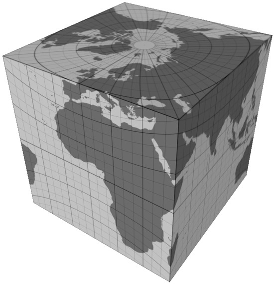
Figure 1.
Hexahedral projection: projecting the Earth’s surface onto a cube.
A practical implementation involves numerous additional transformation steps, allowing us to refer to it as a transformation pipeline. Figure 2 presents a symbolic depiction of the complete transformation pipeline. This pipeline operates bidirectionally: it must enable the mapping of geodetic coordinates (ϕ, λ) to plane coordinates (x, y, Si) on the corresponding face Si of the cube (forward transformation) and also support the reverse mapping back to geodetic coordinates (inverse transformation). In Figure 2, forward transformation steps are labeled Fi, while inverse transformation steps are labeled Ii. Arrows indicate the flow of the transformation process.
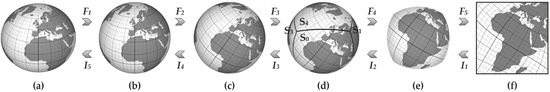
Figure 2.
The complete transformation pipeline of geodata from the geodetic ellipsoidal to the hexahedral coordinate system through six stages: (a) ellipsoid, (b) sphere, (c) graticule system rotation, (d) cube side delimitation, (e) mapping to the front side, and (f) projection onto the plane.
The forward transformation begins by mapping the ellipsoid (Figure 2a) to the sphere (Figure 2b) through the transformation of geodetic latitude to authalic or conformal latitude (F1). Next, an optional rotation of the graticule system (Figure 2c) may be applied (F2) to minimize distortion or to position singularities outside the area of interest. Following this, the appropriate side of the cube (Figure 2d) for the current coordinate is identified (F3), and then that side is mapped (F4) to the front-facing side of the cube (Figure 2e). The final step (F5) involves projecting one-sixth of the sphere’s surface onto a plane (Figure 2f)—this is the narrower definition of hexahedral projection.
The inverse transformation includes the same sequence of steps (Ii), where each step reverses the corresponding forward transformation step, following the relation Ii = F6−i −1.
In hexahedral projections, the unit sphere is commonly projected onto a unit cube. This approach simplifies calculations and results in normalized coordinate values x, y ∈ [−1, 1]. However, it is important to note that the surface area of this unit cube does not match that of the projected sphere. Consequently, when interpreting area distortion, the distortion indicators will show values 6/π (≈1.9099) times higher than the expected values on an equal-area basis.
None of the steps in the transformation pipeline are fixed; the choice of implementation method influences speed, accuracy, and distortion. Consequently, each step is addressed in a dedicated subsection below.
3.1. Mapping an Ellipsoid to a Sphere
Although the Earth’s true shape deviates from a perfect sphere, it is often approximated as such to simplify mathematical calculations. The geoid represents the most accurate model of Earth’s shape by defining mean sea level. However, this model is highly complex and irregular, so it is instead represented as deviations from a smoother, more regular model—the ellipsoid. These deviations are accounted for in terrestrial measurements to align results precisely with a global reference model. Reference ellipsoids have been developed since the late 18th century, culminating in the widespread adoption of the WGS 84 ellipsoid [41], which now underpins most global datasets due to the demands of precise global navigation.
Despite the ellipsoid’s greater accuracy, it can still be cumbersome for many geodetic calculations and is therefore often replaced by a spherical model, which offers higher symmetry and simpler computations. Fortunately, given Earth’s minor deviation from a perfect sphere, spherical formulas can be applied by substituting geodetic latitude with an auxiliary latitude. The choice of auxiliary latitude depends on the property to be preserved: authalic latitude is used to preserve area, while conformal latitude is used when it is essential to preserve angles.
The formulas for auxiliary latitudes were derived and systematized by Adams in 1921 [42] but gained broader recognition after the publication of Snyder’s manual in 1987 [43]. The transformation from geodetic latitude (ϕ) to authalic latitude (β) is given by Equations (1)–(3).
While this transformation is relatively complex, it has a closed-form solution, enabling direct and efficient calculation by avoiding numerical approximations or iterative methods. Adams also defined an approximate series formula, as shown in Equation (4).
However, the inverse transformation—mapping authalic latitude back to geodetic latitude—does not exist in closed form. This calculation instead relies on the series expansion or iterative procedure. The series defined by Equation (4) can be used in this case as well, if ϕ and β are replaced. Adams recalculated the three coefficients in the series expansion.
In his derivations, Adams performed each transformation in several different ways, consistently arriving at the same final formula and relying on the eccentricity of the ellipsoid. Karney [44] demonstrated that significantly greater numerical stability in approximating auxiliary latitudes can be achieved by using the third flattening, n = (a − b)/(a + b), instead of the squared eccentricity, e2 = 1 − b2/a2, where a and b are the semi-major and semi-minor axes of the ellipsoid, respectively. The significance of applying the third flattening in geodesy was established by F. R. Helmert in 1880 [45], who demonstrated its role in achieving faster convergence of the corresponding series. In his work, however, n is not explicitly identified under a specific term but is treated as one of the auxiliary quantities. Even before Helmert, this parameter was used in calculations by Bessel in 1841 [46] and Encke in 1852 [47]. Karney derived sixth-order series expansion coefficients for converting between any two auxiliary latitudes.
Figure 3 illustrates the deviation in approximate authalic latitudes using series expansions with Adams’ three coefficients (Adams 3) and Karney’s three (Karney 3) and six (Karney 6) coefficients. Notably, even with only three coefficients, Karney’s formulas provide an approximation that is nearly two orders of magnitude more accurate. Interestingly, all three approximations show similar divergence near the pole.
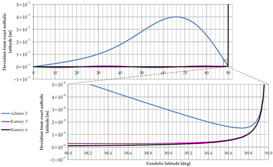
Figure 3.
Deviation of approximations relative to the exact authalic latitude. Comparisons were made between series approximations with three terms (Adams 3 and Karney 3) and a series with six terms (Karney 6). Deviations are presented in meters for the authalic sphere.
Only the forward transformation (from geodetic to authalic latitude) maintains a relatively small deviation. A more substantial issue arises from error accumulation when converting back to geodetic latitude, especially given the lack of closed-form formulas for the inverse transformation. Figure 4 displays the positional error after returning to geodetic latitude (ϕ→β→ϕ).
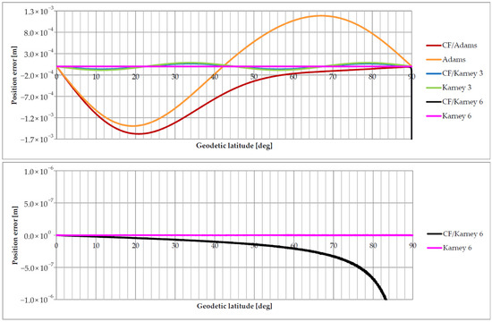
Figure 4.
Error in geodetic latitude after conversion to authalic latitude and back to geodetic latitude, i.e., after successive application of the forward and inverse transformations. The error is expressed in meters for the authalic sphere case. Comparisons were made between cases where a closed-form equation (indicated by CF in the name) is used for the forward transformation and cases where an approximation is applied for both forward and inverse transformations. The number in the method name denotes the number of coefficients used in the series expansions.
Applying Karney’s approximate formula with six coefficients in both the forward and inverse transformations effectively eliminates the positioning error. A comprehensive analysis is available in [44]. Considering the slightly lower complexity and faster computation of forward transformation using series expansion compared to the closed-form expression, this approach is recommended for implementing steps F1 and I5.
As with authalic latitude, only the forward transformation of conformal latitude has a closed-form solution, as defined by Equation (5).
The inverse transformation can be implemented either iteratively or through a series expansion. The series expansion follows the same form as in Equation (4), substituting β with ϕ and ϕ with χ.
3.2. Graticule System Rotation
For most hexahedral projections, it is simplest, both in derivation and application, to orient the cube so that the prime meridian aligns vertically and the equator horizontally, bisecting the front-facing sides (Figure 1), which is referred to as a direct or normal aspect [48,49]. Such an orientation allows the coordinate origin of the graticule system to coincide with that of the local coordinate system of the front-facing side, aligning with the four symmetry axes. This alignment enables the projection to be defined over only a quarter (e.g., QSC and ROS) or even an eighth (e.g., RAN) of the cube side, with the remaining portions derived through symmetry. As a result, consistency is maintained across the cube even in cases where the projection function is not defined over the entire cube side. Distortion may also be reduced when using approximations. Calculating values for only an eighth of the side, then deriving the remaining values through symmetry, minimizes the loss of precision that occurs with distance from the origin, as in the case of the RAN projection.
However, a direct aspect may be disadvantageous in terms of the placement of singularities and the distribution of distortion relative to areas of interest. In the conformal hexahedral projection, singularities appear at the cube’s vertices. Since this projection is often used to represent and analyze ocean currents, it is logical to orient the cube so that its vertices lie over landmasses. Conversely, if the focus is on minimizing distortion over landmasses, the cube should be oriented so that its edges intersect large bodies of water.
Creating an oblique aspect of the projection by rotating the graticule system constitutes the second step (F2) in the forward transformation pipeline. The orientation of a rotated (pseudograticule or metagraticule) system is typically defined by the geographic coordinates of the north pseudopole (or metapole). However, this definition accounts for only two rotations, implicitly setting the third to zero. A detailed analysis and complete derivation of formulas for converting geographic to metageographic coordinates are provided in [50]. When coordinates are converted from geographic to Cartesian, which can simplify the next step in the pipeline, the transformations from coordinates v to metacoordinates v′ (Rfwd) and vice versa (Rinv) are given in Equations (6) and (7). The parameters dϕ, dλ, and dρ represent the rotation angles about the X, Y, and Z axes, respectively.
The optimal rotation angles are primarily determined by the distortion reduction objective and the choice of hexahedral projection in step F5. An example of minimizing continental mass distortion in the MSC projection is provided in [51]. Rotating the graticule system is an optional step in the transformation pipeline that increases projection complexity; therefore, it can be omitted if not necessary.
3.3. Cube Side Determination
The projection of a sphere onto a cube is typically represented as six gnomonic projections on the planes of the cube’s sides. For simplicity, the projection formulas are usually derived for a single plane, often the front-facing one. To project the entire sphere, the graticule system is rotated so that each side of the cube successively aligns with the frontal plane. Therefore, the third step in the forward transformation pipeline (F3) is to determine which side of the cube the given geographic coordinates (ϕ, λ) fall on, followed by transforming that side to the front-facing position (F4). Figure 5 illustrates the edges of the cube projected onto the globe (left) and in the Plate Carrée projection (right) in a case where the rotation of the graticule system is omitted.
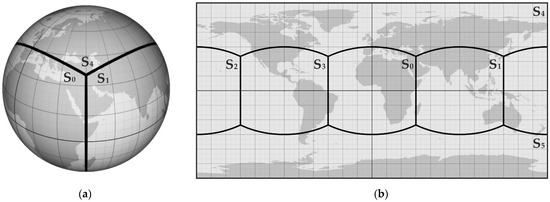
Figure 5.
The edges of the cube projected onto the globe (a) and in the Plate Carrée projection (b).
There are several methods to determine the side of the cube to which a point with specified geographic coordinates belongs. In the following subsections, we will examine several frequently used approaches.
3.3.1. Direct Approach
The simplest approach to solving this problem can be deduced from Figure 5. For simplicity, let us consider the direct aspect of the projection. It is evident that the side edges of the cube align with the geographic meridians. Let S0 denote the front-facing side, i.e., the side whose center coincides with the center of the geographic grid. A point with polar coordinates (ϕ,λ) belongs to side S0 if and only if –π/4 < φ < π/4 and −Θ(λ) < ϕ < Θ(λ). For the sake of simplicity, we will temporarily disregard the latitude constraint. Determining which side of the cube a point belongs to can be accomplished based solely on the interval of the geographic longitude, and the reduction to side S0 is performed using the formula λ′ = λ − kπ/2, where k represents the ordinal number of the cube side to which the point belongs.
We can assume that a point initially belongs to sides S0 to S3, which holds true in two-thirds of the cases. The plane coordinates (x, y) can then be computed using the forward transformation formulas for the respective projection. If the resulting y-coordinate falls within the range [−1, 1], the assumption is correct, and no further calculations are needed. If y > 1, the point belongs to side S4, and if y < −1, the point belongs to side S5. In these cases, the coordinates need to be rotated about the global X-axis by either –π/2 or π/2, respectively, and the forward transformation formulas applied once again. Importantly, this method does not require knowledge of the specific function Θ(λ), which defines the upper and lower boundaries of the front-facing cube side.
This approach results in varying computational times for coordinate conversion depending on the cube side to which a point belongs. The transformation of side S4 to side S0 is performed using Equations (8) and (9), while the transformation of side S5 to S0 follows Equations (10) and (11). In the following formulas, (ϕ, λ) denote the global geographic coordinates, while (ϕS4, λS4) and (ϕS5, λS5) represent the pseudogeographic coordinates corresponding to sides S4 and S5, respectively.
Since the pairs of Equations (8) and (9), as well as (10) and (11), are mutually inverse, their successive application returns the original coordinates.
The increase in coordinate conversion time for sides S4 and S5, in addition to the required rotation of the coordinate system, is primarily influenced by the need to apply the forward transformation of the chosen projection twice. This effect is particularly pronounced in complex projections. Nonetheless, this issue can be mitigated by calculating the upper (Θ(λ)) and lower (−Θ(λ)) bounds of the front-facing side and determining whether the point lies within these bounds before applying the appropriate projection. The bounds are calculated using Equation (12).
This additional step increases the forward transformation time for sides S0 to S3 but reduces it for S4 and S5. However, it enables the application of this method for determining cube sides across all projections. Specifically, the RAN projection is undefined over an entire cube side, making it even more impractical to define beyond its boundaries. Additionally, in the EVR and SSS projections, the y-coordinate always remains within the boundaries of the side. Therefore, checking the upper and lower bounds of the front-facing side provides a more universal solution while also improving the average forward transformation time for most hexahedral projections.
Regardless of how the forward transformation is implemented, the inverse transformation remains the same for this approach. For sides S0 to S3, the calculated longitude is adjusted solely according to the formula λ = λ′ + kπ/2, where k represents the ordinal number of the side. In contrast, for sides S4 and S5, rotation around the global X-axis is applied by ±π/2, as previously defined in Equations (8)–(11).
3.3.2. Lat/Lon to Cartesian Conversion Approach
A significant performance issue with the direct approach to determining the cube side is the need to rotate sides S4 and S5 when aligning with the front-facing side. This can be completely avoided by using Cartesian coordinates instead of geographic coordinates. In the Cartesian coordinate system, a rotation by kπ/2 reduces to simply swapping coordinate axes and/or changing the sign of one axis. For example, when mapping side S1 to S0, the X-axis becomes −Z, the Y-axis remains unchanged, and the Z-axis becomes X. Prior to rotation, the cube side to which a point belongs is determined by identifying the coordinate with the maximum absolute value. By normalizing all three Cartesian coordinates to this maximum absolute value, determining the side is simplified to verifying whether the relevant coordinate is 1 or –1.
The advantage of this approach over the previous (direct) method is that the duration of inverse transformations remains consistent across all sides of the cube, with a similar uniformity in forward transformations. Additionally, when considering the average time for either forward or inverse transformations across all sides, the lat/lon to Cartesian conversion method generally yields better results for most projections. However, this cannot be universally applied to all projections. While determining the cube face may seem like a minor detail, this choice can significantly impact performance, highlighting the importance of careful consideration.
3.3.3. Other Approaches
The previous two approaches do not encompass all possibilities for determining the appropriate cube face and aligning it with the front-facing side. An alternative method, presented in [32], also utilizes Cartesian coordinates but employs the vector product instead of relying on the maximum absolute coordinate value. Six unit vectors vi are predefined, with each pair orthogonal and located in one of the coordinate planes. Each vector vi defines a plane, and the scalar product of the position vector with vi determines on which side of that plane the point lies. By combining conditions for four such planes, a pyramidal region is formed with its apex at the origin and its base on one of the cube faces.
This method is implemented within the graphics processing unit (GPU) shader for the projection, as described in [32], where scalar product calculations are efficiently handled using shading language functions. When implemented on a central processing unit (CPU) using double precision arithmetic and without hardware-accelerated functions, this approach is slightly more complex and, consequently, slightly slower than the previous method.
3.4. Mapping a Portion of the Sphere onto a Cube Face
The final step (F5) in the forward pipeline involves mapping one-sixth of the sphere’s surface onto a plane, specifically onto a cube face. This step forms the core of the hexahedral projection and has the greatest influence on the distortion introduced during the mapping. Consequently, numerous implementations have been developed over the past 50 years, as no single approach has been able to optimize all parameters critical for various applications.
Hexahedral projections can be categorized into three groups based on their derivation methods and defining characteristics:
- Line-smoothness-preserving projections;
- Equal-area projections;
- Compromise projections.
3.4.1. Preserving Line Smoothness
Preserving line smoothness refers to the property whereby lines that are continuous and smooth on the surface of the sphere retain this characteristic when projected onto the plane. This is crucial for analyzing global air and water flows, which has driven the development of various hexahedral projections [8,22,23]. It is also vital in maritime and aviation navigation, as it ensures accurate course tracking and facilitates the planning of routes with consistent direction. Hexahedral projections that preserve line smoothness can be further classified into two subtypes:
- Conformal projection;
- Relaxed projections.
In a conformal projection, two lines that intersect on the surface of a sphere at a given angle will intersect at the same angle in the projection onto the plane. This property is valuable in geodetic applications and the mapping of small areas, as it preserves the shapes of buildings and infrastructure. However, conformality introduces areal distortion. As you move away from the projection center, shapes tend to enlarge. Furthermore, in the case of hexahedral projections, eight singular points appear at the vertices of the cube, where area distortion becomes infinite.
To mitigate the effects of areal distortion, projections derived from the conformal projection were developed with relaxed constraints. One approach involves rescaling the coordinates after the original conformal mapping [23]. Relaxed projections offer a more uniform distance between meridians and parallels, while maintaining line smoothness, but at the cost of breaking conformality. This is clearly illustrated in Figure 6. The singularity at the cube’s vertices persists even in relaxed projections. In the analysis presented in the following sections, the RAN projection represents the conformal hexahedral projection, while the ADC projection represents relaxed projections.
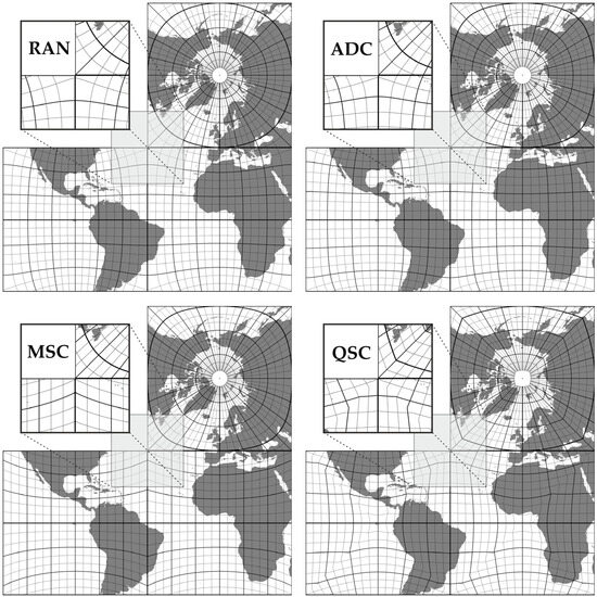
Figure 6.
Comparison of graticule systems in RAN, ADC, MSC, and QSC projections. In the conformal projection (RAN), all lines remain inherently smooth. Relaxed projections (ADC) preserve line smoothness with more uniform spacing along the side edges. Compromise projections (MSC) display sharp line breaks at the cube edges, while in equal-area projections (QSC), line breaks are visible along both the edges and diagonals.
Figure 6 illustrates how the smoothness of lines is disrupted along the edges of the cube in compromise projections, as demonstrated by the MSC projection example. In equal-area projections, this effect extends beyond the edges, with lines often breaking along the side diagonals, as shown in the QSC projection.
3.4.2. Preserving Area
An equal-area projection, also known as an equivalent or authalic projection, is one that conserves surface area in mapping. These projections are widely used in statistical analysis and the visualization of spatial distributions, as they retain the apparent density of the represented phenomena. Hexahedral equal-area projections can be categorized into three types:
- Fully edge-continuous equal-area projections;
- Partially edge-discontinuous equal-area projections;
- Approximate equal-area projections.
Fully edge-continuous equal-area projections have edges that are all C0 continuous. This means lines from one side of the cube extend to the adjacent side without gaps, though these transitions lack smoothness. Typically, these projections map part of the sphere onto a quarter of a cube face, specifically onto a right-angled triangle whose catheti align with the diagonals of the face (see Figure 7). The remaining three-quarters of each face are generated by mirroring this initial quarter, achieved through changes in sign and/or swapping the plane coordinates x and y. However, the continuity along these triangle catheti is only C0, and the transitions are significantly sharper than those at the edges of the cube.
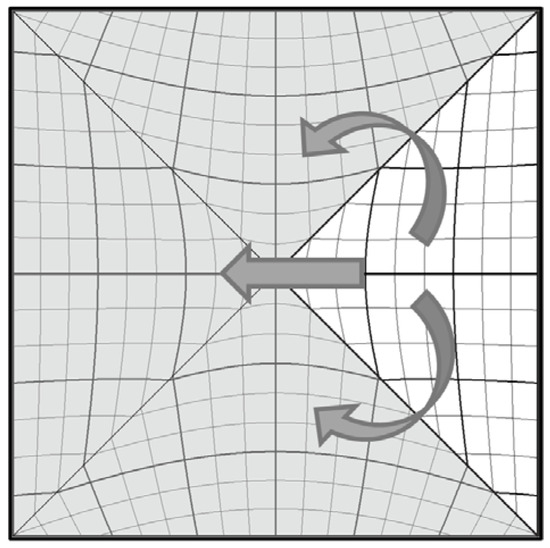
Figure 7.
The projection is defined only for one quarter of the page—specifically, the right-angled triangle with its vertex at the center of the page (white triangle on the right). The remaining three quarters (gray triangles indicated by arrows) are obtained through mirroring.
Partially edge-discontinuous equal-area projections do not maintain even C0 continuity at their edges. An example is the ARV projection, where noticeable misalignment occurs along four edges of the cube (Figure 8). This results from asymmetry in the transformation relative to the page diagonals. Angular distortion increases more rapidly along the Y-axis, causing discontinuities along the upper edges of the side faces (S1 and S3). Due to this limitation, the ARV projection is often disregarded and excluded from analyses [20,21].
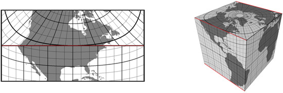
Figure 8.
Discontinuities along certain cube edges in the ARV projection. Red indicates edges where discrepancies exist between adjacent sides. The left image shows a magnified view of the discontinuity crossing the North American continent, while the right image displays the locations of the discontinuous edges on the cube.
Approximate equal-area projections, as the name suggests, are not strictly equal-area but permit minor deviations. The standard deviation of areal distortion serves as a measure of this deviation. For the QLSC projection, this deviation is below 2%, qualifying it for this category.
In the analysis presented in the following sections, the QSC/ROS projection represents fully edge-continuous equal-area projections, the ARV projection represents partially edge-discontinuous equal-area projections, and the QLSC projection represents approximate equal-area projections. Although QSC and ROS have different derivation procedures and formulas, they are essentially the same projection, as shown by their equivalent distortion diagrams.
3.4.3. Compromise Hexahedral Projections
Hexahedral projections that neither preserve line smoothness nor area are commonly categorized as compromise projections, as they achieve a balance between conformality and equivalence. Notably, this is the largest class of hexahedral projections, as these projections provide not only an aesthetically balanced display but are also widely applicable across diverse use cases. Moreover, by not being constrained to strict requirements for conformality or area preservation, they allow for extensive optimization of specific attributes, resulting in a virtually unlimited range of possible forms.
Hexahedral projections, in terms of their adaptability to distortion, can be classified into:
- Strict projections;
- Parametric projections.
In this context, ‘strictness’ refers to mapping functions that are fixed and independent of external parameters. The simplest examples in this category are the TSC and MSC projections. When the lat/lon-to-Cartesian conversion method (Section 3.3.2) is applied in step F3 of the forward transformation pipeline, step F5 is omitted for the TSC projection. Normalizing the Cartesian coordinates then produces a standard gnomonic projection, which defines the TSC. However, if a direct approach (Section 3.3.1) is employed in step F3, step F5 becomes more complex and is governed by Equations (13) and (14).
Conversely, the direct approach provides a natural basis for defining the MSC projection, as the x-coordinate in this projection directly corresponds to longitude. With a reduction to the interval [−1, 1], only a division by π/4 is necessary. In this case, step F5 for the MSC projection is governed by Equations (15) and (16).
When the lat/lon-to-Cartesian conversion method is applied in step F3, both x and y (denoted by a) are computed using Equation (17).
The preceding examples clearly illustrate how the choice of implementation method for step F3 in the forward transformation pipeline impacts the overall complexity of the projection.
Parametric projections are derived from strict projections by introducing adjustable parameters to help balance distortion. For ease of use, these projections typically include only a single parameter, which appears as a constant in the projection formulas. The simplest example is the TAN projection, which is based on the MSC projection. Equation (17) is modified to include the parameter p, as shown in Equation (18). When p = 1, the TAN projection reduces to the MSC projection.
Each parametric projection represents a continuous spectrum of distinct projections determined by the parameter value. Figure 9 illustrates the appearance of the S0 side in the TAN projection for various values of the parameter p.
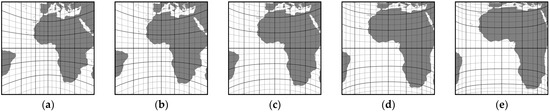
Figure 9.
Appearance of side S0 in the TAN projection for selected values of parameter p: (a) p = 0.1, (b) p = 0.5, (c) p = 1.0, (d) p = 1.5, and (e) p = 2.0.
The analysis in the following sections considers the strict projections CCM, KSC, MSC, OTC, POL5, S2Q, and TSC, along with the parametric projections ALG, EVR, LOG, SSS, TAH, and TAN. The determination of the optimal value for the parameter p is discussed in detail in Section 4.3.
4. Distortion
A spheroidal surface, such as that of the Earth, possesses intrinsic curvature, whereas a map is a flat surface with zero Gaussian curvature. The impossibility of perfectly mapping a sphere onto a plane was first demonstrated by Euler half a century before Gauss’s Theorema Egregium [52], in his work De repraesentatione superficiei sphaericae super plano [53]. Gauss later showed that curvature is an invariant property that cannot be altered through any isometric mapping. Consequently, since a curved surface cannot be flattened without modifying distances, angles, or areas, every map projection necessarily introduces some form of distortion. This section explores commonly used distortion metrics, methods for visualizing distortion, and strategies for selecting the parameter p in parametric projections to optimize distortion.
4.1. Distortion Metrics
At the end of the 19th century, the French cartographer Nicolas Auguste Tissot published an analysis of distortions in map projections that has become a foundational reference in the field and remains in use today. Tissot [54] demonstrated that distortions inherent in map projections transform an infinitesimal circle on the Earth’s surface into an infinitesimal ellipse on the map. The parameters of this ellipse characterize the type and magnitude of the distortion.
In conformal projections, the ellipses are circles, and their size reflects areal distortion. In equal-area projections, the ellipses maintain the same area as the original circles on the Earth, while their flattening represents angular distortion. This ellipse, which serves as an indicator of distortion, is referred to as Tissot’s indicatrix.
Given the major (a) and minor (b) semi-axes of the indicatrix, the two key distortion metrics at a specific point [43] can be determined as follows:
- Angular distortion:
- Areal scale:
Angular distortion represents the ratio of the major to minor semi-axes of the indicatrix, while the areal scale denotes the ratio of the indicatrix area to the area of the corresponding circle on the Earth’s surface.
The third commonly used metric based on the indicatrix semi-axes is the maximum angular deviation, which represents the largest difference between the angle of intersection of two lines on the Earth’s surface and the angle between their projections. It can be calculated using Equation (21).
Although the semi-axes of the indicatrix represent the maximum and minimum scale factors at a given point, their ratio (α) serves as a measure of angular distortion, and there exists a functional relationship between α and ω. Specifically, dividing both the numerator and denominator in Equation (21) by b and applying the transformation from Equation (19) yields:
Solving Equation (22) for α, we obtain:
Thus, both α and ω serve as measures of angular distortion, but α is preferable because it is dimensionless, can be considered multiplicative in a general sense [55], and is comparable to areal scale.
Since the linear scale depends entirely on α and σ, and there is a strong linear correlation between the linear scale and a linear combination of angular and areal distortion [56], α and σ can fully describe map distortions at the infinitesimal scale [55].
Tissot’s formulas underpin many modern distortion metrics. For example, Lambers [21] introduces DA and DI metrics. DA normalizes the areal scale by 6/π, ensuring a value of 1 for equal-area projections. While equal-area projections preserve area by definition, exact matching requires mapping the unit sphere to a cube with side length , complicating derivations and coordinate handling. To simplify, we can define equal-area mapping as proportional area preservation, characterized by there being no deviation in the areal scale factor. Since DA is simply a normalized areal scale factor, it will not be discussed further. Similarly, the DI metric, which is identical to angular distortion, is also not used for evaluating hexahedral projections.
Another metric derived from Tissot’s formulas is the grid oversampling factor (GOF), introduced by Bauer-Marschallinger et al. [57]. GOF quantifies the local oversampling of data that occurs when generic satellite images are projected onto a regular raster grid. It is defined by Equation (24) as the ratio of areal scale (σ) to the square of the global minimum scale factor (bmin):
The parameter bmin, which represents the minimum value of the indicators’ minor semi-axes, is a constant for a given projection, making GOF a normalized measure of areal distortion. Consequently, spatial distribution diagrams (Section 4.2.3) for GOF and σ are identical, since both metrics vary in the same manner for a given projection. However, the average and maximum values of GOF are important for inter-projection comparisons and are analyzed in the following sections.
GOF quantifies sampling efficiency. A GOF > 1 indicates oversampling, leading to data redundancy, increased storage requirements, and unnecessary computational overhead. Conversely, a GOF < 1 signifies undersampling, resulting in a loss of information. Ideally, GOF values should be close to but greater than 1, as this corresponds to minimal distortion.
4.2. Visualizing Distortion
The distortion effect is generally apparent on the map, but interpreting it requires an experienced observer who can compare the current map with reference maps of known distortion. Even then, distortion effects are typically noticeable only on smaller-scale maps, particularly when the changes are not subtle.
4.2.1. Graticule System and Continental Outlines
The lines of the graticule system have a distinct and recognizable structure, making any deformation—such as bending or the failure of meridians and parallels to intersect at right angles—immediately apparent. Additionally, our perception is shaped by familiarity with the actual shapes and proportions of continents. When these shapes appear distorted or out of scale, deviations from their expected appearance are easily noticed. Therefore, utilizing the graticule system and continental outlines to identify distortion effects is the most intuitive and effective approach. Figure 10 illustrates this technique.
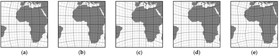
Figure 10.
Layout of the graticule system and continental outlines on the S0 side of selected hexahedral projections: (a) RAN, (b) ADC, (c) TAN (p = 0.5), (d) MSC, and (e) QSC.
On the far left is the RAN projection, which is known to be conformal. This is further evidenced by the perpendicular intersection of meridians and parallels. None of the other projections exhibit similar continental shapes, indicating that they are not conformal.
The TAN projection (for p = 0.5) displays a relatively regular shape of the Iberian Peninsula, but conformality can be ruled out based on the behavior of the parallels. In the conformal hexahedral projection, while the parallels may curve across the cube face, they align parallel at the edges and intersect the side edges at right angles.
The ADC projection exhibits this graticule characteristic, yet the Iberian Peninsula is noticeably stretched in the east-west direction. This suggests that the projection preserves smoothness of the lines but is not conformal.
In all hexahedral gnomonic projections, the meridians on the S0–S3 sides are perfectly vertical and mutually parallel. This property is shared by the majority of hexahedral projections that are neither conformal nor equal-area. However, it cannot be generalized to this class of projections, as there are exceptions where meridian parallelism does not hold—for instance, in the KSC projection—or where it holds for an equal-area projection, such as ARV.
When parallels and meridians appear as broken lines rather than smooth curves, the projection is likely equal-area. This characteristic is evident in the QSC projection shown in Figure 10. The distortion of shapes is highly pronounced, making the map visually unappealing. Such distortion typically indicates a deliberate design choice, often to achieve the equal-area property. However, simply observing the map does not confirm area preservation; it only suggests the possibility. Therefore, additional methods of distortion visualization are necessary to verify this property.
4.2.2. Tissot’s Indicatrices
Tissot’s indicatrices are commonly used to represent distortion on maps. Figure 11 displays the same projections shown in Figure 10, but with Tissot’s indicatrices overlaid. These indicatrices are typically plotted over the continental outlines to contextualize the distribution of distortion relative to known locations. In the case of hexahedral projections, distortion is solely dependent on the position within each side and remains consistent across all sides of the cube. Therefore, Figure 11 includes only the cube’s side frame and the distribution of indicatrices.
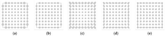
Figure 11.
Tissot’s indicatrices overlaid on a cube face for selected hexahedral projections: (a) RAN, (b) ADC, (c) TAN (p = 0.5), (d) MSC, and (e) QSC. The shapes along the face diagonals in the QSC projection were obtained using a numerical method, as Tissot’s formulas cannot be applied at discontinuities.
Tissot’s indicatrices provide a straightforward and intuitive way to assess distortion. If all indicatrices are circles, regardless of their size, the projection is conformal. If all indicatrices have the same area, regardless of their shape, the projection is equal-area. The flatter the indicatrix, the greater the angular distortion, while its orientation indicates the direction of stretching or contraction.
Despite their usefulness, the application of indicatrices has several drawbacks, as illustrated in Figure 11. First, in the case of singularities, the indicatrices become infinitely large and cannot be displayed. This is why the indicatrices at the corners of the cube faces for the RAN and ADC projections are absent. Second, since indicatrices are drawn at only a limited number of points, irregularities in the projection can easily go unnoticed. For example, if the number of samples were even both horizontally and vertically in the QSC projection, the irregularities along the diagonals would not be visible. Third, it is challenging to accurately estimate the size of the indicatrices to confirm that they all represent the same area. Moreover, Tissot’s formulas cannot be applied at discontinuities, such as along the face diagonals of the QSC projection. In these cases, numerical methods can be used to determine the shape into which the infinitesimal circle is mapped, or the shape can be reconstructed as a composition of segments of the indicatrix bounded by discontinuities [58].
4.2.3. Distortion Spatial Distribution Diagrams
A more detailed representation of distortion is provided by diagrams showing its spatial distribution. These diagrams illustrate distortion variation by using color gradients across the cube faces to reflect the observed values. There is no consensus on the design of these diagrams. Figure 12 illustrates several color-coding variations. On the far left, the simplest form using grayscale is shown, as employed in [11]. Blue and red hues are commonly used to highlight changes in areal scale, with varying interpretations. For instance, a white-to-red transition can represent area shrinking and a white-to-blue transition area expansion [20], or the reverse, with an additional black transition to enhance diagram sharpness [21]. On the far right, the diagram employs discrete grayscale shading with 20 levels, where areas in the same shade are outlined by isolines.
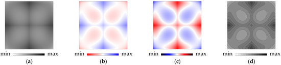
Figure 12.
Distortion spatial distribution diagrams for the EVR projection, with variations in color-coding: (a) grayscale, (b) red-to-white-to-blue gradient, (c) black-to-blue-to-white- to-red-to-black gradient, and (d) discretized grayscale with isolines.
Color-coded diagrams with multi-color transitions are used only for areal distortion, where the reference value indicating no distortion lies in the middle of the range. In contrast, for angular distortion metrics and GOF, characteristic values are at the lower bound of their intervals (GOF ≥ 1, α ≥ 1, ω ≥ 0), making multi-color transitions less meaningful. Instead, diagrams with discretized gray levels and isolines are preferred to maintain consistency across all distortion types.
The inclusion of isolines in spatial distribution diagrams is particularly beneficial because they:
- Highlight small variations in value, with isolines marking every 5% change;
- Clearly indicate the direction and intensity of distortion growth (denser isolines correspond to faster growth);
- Allow for an approximate determination of value ranges by counting isolines from the lightest to the darkest area;
- Facilitate the assessment of projection quality by examining the extent of uniform areas shaded similarly.
Distortion spatial distribution diagrams are a powerful tool for analyzing the characteristics of a projection and for recognizing the same projection expressed using different formulas. For example, QSC and ROS represent different formulations of the same projection, a conclusion that cannot be drawn solely from examining their mathematical expressions. While their computational speed, accuracy, and numerical stability may differ significantly, the distortion diagrams are identical across all types of distortions.
Figure 13 presents examples of distortion spatial distribution diagrams for the S2Q projection. A notable similarity is observed between the maximum angular deviation (ω) and angular distortion (α) diagrams, as well as between areal scale (σ) and the GOF. Moreover, the spatial distribution diagrams for σ and GOF are identical for each projection, while those for ω and α differ slightly only in isoline density. A pair of spatial distribution diagrams—one for angular distortion and one for areal distortion—forms a distinct signature that can uniquely identify a projection, much like fingerprints.
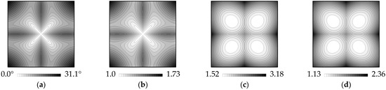
Figure 13.
Distortion spatial distribution diagrams for the S2Q projection: (a) maximum angular deviation (ω), (b) angular distortion (α), (c) areal scale (σ), and (d) grid oversampling factor (GOF).
4.3. Optimizing Parametric Hexahedral Projections
Parametric projections are commonly derived by adjusting the grid generated by standard projections. By varying a single parameter, these projections aim to achieve a more uniform point distribution and reduce distortion. This section examines six parametric projections: ALG, EVR, LOG, SSS, TAH, and TAN, starting with the parameter values proposed by their authors to understand the motivations behind their development.
4.3.1. Optimizing Areal Distortion
In previous studies [20,21,38], the parameterization of compromise hexahedral projections has consistently aimed to minimize areal distortion, employing variational and minimax methods [59]. The variational method minimizes dispersion by reducing the standard deviation, while the minimax method minimizes the ratio of extreme values for multiplicative metrics or the difference of extreme values for additive metrics.
Figure 14 illustrates the variation of the mean value (σave), the ratio of maximum to minimum (σm/m), the arithmetic standard deviation (σSD), and the geometric standard deviation (σGSD) for the TAN projection. The displayed metric values are normalized by their minima. Although σGSD is the appropriate measure of dispersion for multiplicative metrics [55,60], σSD is also considered, as previous studies on parametric projections used it for optimization [20,21]. The difference between the parameter p values minimizing σSD and σGSD is negligible and not discernible in Figure 14, so Table 1 provides the exact p values corresponding to the minima of each metric.
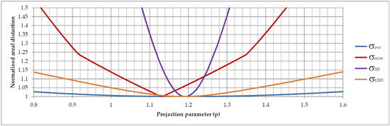
Figure 14.
Normalized dependence of areal distortion metrics on the projection parameter p for the TAN projection.

Table 1.
Optimal parameter p values for minimizing σm/m, σGSD, σSD, and σave.
The metric curves for all parametric projections exhibit similar shapes and distributions of minima, with the primary difference being the shift in the parameter range where the minima occur. Table 1 presents the optimal p values for the four minimization strategies (σm/m, σGSD, σSD, and σave). For all observed parametric projections, the following relation holds: popt(σm/m) < popt(σave) = popt(σGSD) < popt(σSD). The equality of popt(σave) and popt(σGSD) suggests that the variational method, which minimizes the geometric standard deviation, also minimizes the mean value. This further reinforces the geometric standard deviation as a valid measure of dispersion for areal distortion. Moreover, this confirms that, objectively, only two optimization methods for areal distortion exist—the variational and minimax approaches.
4.3.2. Optimizing Angular Distortion
Although the primary goal of projection parameterization is to optimize areal distortion, adjusting the parameter p also influences other types of distortion. Figure 15 illustrates how normalized angular distortion metrics vary with p using the TAN projection as an example. Since αmin = 1, αm/m and αmax are equal, so only αmax is shown. Additionally, it is worth noting that for all gnomonic hexahedral projections, αmax is approximately 1.732. The figure shows that in parametric projections, αmax remains nearly constant up to a certain threshold of p, making the minimax method unsuitable for optimizing angular distortion in these projections.
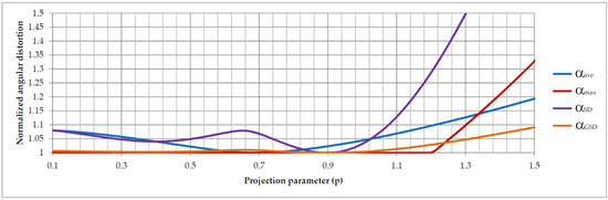
Figure 15.
Normalized dependence of angular distortion metrics on the projection parameter p for the TAN projection.
A notable characteristic of parametric projections is that αGSD lacks a pronounced minimum, exhibiting only minor variations across a broad range of p, whereas αave does have a clear minimum. Therefore, αave is used for optimization. For all parametric projections, it is important to note that popt(αave) is always smaller than popt (σm/m). The optimal values of p for minimizing αave across all parametric projections are provided in Table 2.
Table 2.
Optimal parameter p values for minimizing αave.
4.3.3. Optimizing GOF
Due to the distinct shape of the curves describing the relationship between the grid oversampling factor (GOF) metrics and the parameter p, the minima of GOFave and GOFGSD are significantly offset, as shown in Figure 16. Optimizing GOFave simultaneously minimizes both GOFmin and GOFmax, making it arguably the most suitable optimization approach. For all parametric projections except EVR, GOFmin = 1 over a wide range of p, which extends up to the point where GOFave reaches its minimum. This provides additional justification for prioritizing the optimization of GOFave.
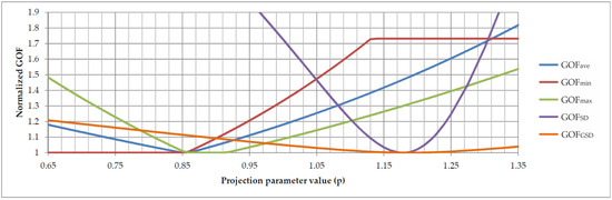
Figure 16.
Normalized dependence of GOF on the projection parameter p for the TAN projection.
Alternatively, if a more uniform sampling factor is preferred, even at relatively high values, the variational method is the appropriate choice. The parameter values at which the minima of GOFSD and GOFGSD occur are very close. However, the GOFSD curve is significantly steeper, enabling a more efficient determination of the optimal p. Table 3 summarizes the optimal parameter values for GOF optimization.
Table 3.
Optimal parameter p values for minimizing GOFave and GOFSD.
4.3.4. Parametric Projection Optimization Summary
The discussion above highlights that parametric projections can be optimized according to several criteria, with multiple aspects to consider even within a single criterion. As a result, each parametric projection with a different value of the parameter p can be regarded as a distinct projection. To streamline the selection process for the optimal hexahedral projection and facilitate the presentation of results in the corresponding tables, a single representative is chosen for each parametric projection.
The optimal parameter value is determined based on a ranking that prioritizes the minimization of angular distortion, areal distortion, and GOF. Based on Table 4, it can be inferred that the optimal placement in the ranking, according to the distortion criterion, is achieved through minimax optimization of areal distortion, specifically applying the parameter popt (σm/m). Experimental results validate this choice, and this parameter value will therefore be used in the next chapter to determine p for parametric projections during the ranking process.
Table 4.
Summary of optimal parameter p values.
5. Evaluation and Ranking of Hexahedral Projections
It is well established that no ideal projection exists; each seeks to optimize specific mapping aspects or strike a balance between competing requirements. This section evaluates hexahedral projections based on multiple criteria and introduces a ranking designed to provide recommendations for specific applications while identifying the most versatile hexahedral projection. The ranking was determined using the mid-rank procedure.
Given the diversity and heterogeneity of the criteria—encompassing both qualitative and quantitative aspects—ranking emerged as the most practical and effective method for comparing hexahedral projections. While ranking has been used previously, such as in the comparison of candidate digital elevation models [61], the approach introduced here enhances the methodology by employing a multilevel structure. This system organizes the evaluation into aspects, criteria, and overarching criteria classes, offering a more systematic and comprehensive framework for comparison.
The ranking process began with individual rankings for specific aspects within each criterion, such as the mean value of angular distortion. These rankings were then aggregated to produce an overall rank for each criterion; for instance, the rank for angular distortion was derived by summing the ranks for its mean value, maximum value, and standard deviation. Finally, the rankings for individual criteria were combined into composite ranks for broader criteria classes. For example, the distortion metrics class rank was calculated by aggregating the ranks for areal distortion, angular distortion, and the grid oversampling factor (GOF).
To facilitate evaluation, the criteria for map projections are grouped into three main classes:
- Structural properties;
- Numerical properties;
- Distortion metrics.
5.1. Structural Properties
Structural properties refer to the discrete geometric characteristics of projections. A discrete property is defined as a characteristic that does not have a numerical value but belongs to a specific category or class. The most commonly discussed structural properties of polyhedral map projections—projections whose projection planes align with the faces of regular polyhedra—are:
- Continuity along edges and diagonals;
- The presence of singularities;
- Symmetry of faces.
5.1.1. Continuity Along Edges and Diagonals
Continuity along edges is an important structural property, as it allows for the seamless display of unfolded maps by connecting the faces of the polyhedron in planar space. Beyond visual appeal, continuity ensures data consistency and enables accurate analysis of areas intersected by edges. Statistical analyses require C0, while flow analyses demand C1 continuity.
Based on this criterion, hexahedral projections are ranked first by the class of continuity (C1—continuity of the first derivative with smooth transitions, C0—continuity with abrupt transitions, and D—discontinuity) and second by the number of edges and diagonals where the lowest level of continuity occurs. The ranking results for this criterion are provided in the ‘REC’ column of Table 5.
Table 5.
Ranking of projections based on structural properties, including edge continuity (EC), presence of singularities (PS), and face symmetry (FS), with an overall ranking score (∑R).
5.1.2. Singularities
Singularities are points or lines where the projection exhibits infinite or undefined values, leading to extreme distortion, numerical instability, and unsuitability for certain applications. Most hexahedral projections are free of singularities. Singularities occur only in the conformal projection and its derivatives, referred to as line-smoothness-preserving projections in Section 3.4. These singularities are located at the cube’s vertices, resulting in eight points to be avoided during analysis, along with as much of the surrounding area as possible.
The ranking for this criterion is based solely on the presence (T) or absence (F) of singularities. The results of this ranking are provided in the ‘RPS’ column of Table 5.
5.1.3. Face Symmetry
While the symmetry of a projection with respect to the coordinate axes and the diagonals of the cube faces does not have as drastic consequences as singularities or discontinuities, a higher degree of symmetry remains a desirable property for several reasons.
First, symmetry allows the projection to be defined on only a portion of a cube face, which can then be mirrored along the axes of symmetry to cover the entire face. This approach is used in the RAN and ADC projections, where the complex mapping function is defined on a single octant. Second, when using an approximation for mapping, symmetry enables focusing on the region of the face where precision is highest. Third, symmetry along the face diagonals can sometimes simplify implementation, as the mapping function becomes identical for both coordinates. Finally, a higher level of symmetry can also facilitate faster mapping of the entire face, as transformations are applied to only a portion of the face, while the remaining coordinates are derived by simply changing the sign of one or both coordinates.
The ranking for this criterion is based solely on the number of symmetry axes (with higher values indicating better performance). The ranking results for this criterion are shown in the ‘RFS’ column of Table 5.
5.1.4. Structural Evaluation Summary
Due to the limited number of discrete values for the tested criterion, differentiation between individual projections is minimal, resulting in large groups and strong correlations. Within the structural properties class, compromise projections achieved the highest rankings. Conversely, projections that preserve conformality or the equal-area property—or are derived from such projections—are positioned toward the bottom of Table 5. This class of criteria highlights the reasons behind the growing popularity of compromise projections.
5.2. Numerical Properties
Numerical factors play a crucial role in evaluating map projections, as they directly impact the practical use of projections in geographic information systems and applications handling large datasets. In this context, the key criteria are:
- Execution speed of forward and inverse transformations;
- Precision of transformations.
The execution speed of forward and inverse transformations is particularly critical in geodata reprojection and other applications involving coordinate system changes or processing of large datasets. This speed is influenced by the mathematical complexity of the projection and the level of algorithmic optimization, both of which are examined in the analysis of execution performance.
Transformations are not always expressible in closed form. In such cases, iterative methods (e.g., for forward transformations with the OTC and POL5 projections) or series expansions (e.g., for both forward and inverse transformations with the RAN, ADC, and QLSC projections) are employed. The use of approximations impacts not only the precision of the transformations but also the execution speed, depending on the number of iterations or the number of terms in the series expansion.
For performance evaluation, the accuracy of iterative methods was set to 10−13, corresponding to micrometer-level precision on the Earth’s surface. The number of terms in the series expansions adhered to the original specifications provided by the projection authors: 30 terms for the RAN projection and 28 terms for the QLSC projection.
Table 6 presents the mean execution times for forward (column ‘fwd’) and inverse (column ‘inv’) transformations, as well as the maximum absolute error (column ‘err’), measured across 64 million samples uniformly distributed over the S0 side. The tests were conducted on a system equipped with an Intel Core i5-11400H CPU at 2.70 GHz and 16 GB of DDR4 dual-channel memory. The program code was developed in ISO C++ 14, using the Visual Studio 2022 (v143) platform toolset, and executed on a Windows 11 Pro Education operating system.
Table 6.
Ranking of hexahedral projections based on numerical properties: forward transformation time (fwd), inverse transformation time (inv), and positioning error after successive forward and inverse transformations (err). Times (fwd, inv) represent mean values in milliseconds, while error (err) denotes the maximum absolute positioning error. Each projection was evaluated using 64 million measurements on evenly distributed points across the S0 side.
Precise time measurements were obtained using the QueryPerformanceCounter() Win32 profiler API function, which offers a resolution of 0.1 microseconds on the tested platform. The reported values in Table 6 are well below this threshold and represent estimated times derived by measuring the total execution time of 64 million function calls. To prevent compiler optimizations from eliminating unused function calls, the computed results were stored in buffers and subsequently used to perform the inverse transformation.
To account for potential variability in repeated experiments, the results were grouped by value for ranking purposes, ensuring the homogeneity of the groups.
From the perspective of transformation execution speed, as shown in Table 6, the HEALPix projection is the most efficient, while RAN and ADC are the least performant, lagging behind the other projections by two orders of magnitude. Despite both relying on iterative procedures, the OTC forward transformation converges significantly faster than POL5 and achieves accuracy far exceeding its configured threshold while maintaining performance comparable to non-iterative methods.
The precision of the transformations was evaluated by successively applying forward and inverse transformations and measuring the deviation from the initial location. The ‘err’ column in Table 6 reports the maximum absolute errors on the unit sphere.
QLSC and QLSC75, historically significant in the development of hexahedral projections, were excluded from the ranking due to their unacceptably large errors. The ROS projection is also excluded from the comparisons, as it is essentially a variant of the QSC. While mathematically equivalent, they differ in equations, affecting numerical characteristics. ROS has a forward transformation 40% slower but an inverse transformation 10% faster than QSC. More notably, it achieves two orders of magnitude higher precision, with a maximum error of 1.67 × 10⁻¹⁵.
Despite these advantages, QSC is included in the tables due to its earlier introduction and broader recognition in the literature. Functionally, aside from numerical stability and transformation speed, the two projections are identical.
In terms of overall numerical properties, HEALPix stands out as the best-performing projection by a significant margin. It is followed by TSC, the foundational gnomonic hexahedral projection from which many others are derived. Conversely, ADC and RAN lag far behind in performance. While further optimization and precision reduction for these projections may be possible, the gap in complexity compared to other projections is so substantial that their positions in the final ranking would remain unchanged.
5.3. Distortion Evaluation and Ranking
All the variations of hexahedral projections, and projections in general, primarily arise from the need to minimize distortion or strike a balance. Given the distinct nature of the distortion metrics, we will evaluate each criterion separately, specifically:
- Angular distortion (α);
- Areal distortion (σ);
- Grid oversampling factor (GOF).
Each criterion is further divided into three aspects, which are ranked separately:
- Mean value;
- Maximum value;
- Standard deviation.
The mean value represents the central tendency around which the values are distributed, while the standard deviation measures the dispersion of the values. The maximum value indicates the extreme range within which the values vary. Since the minimum values are typically fixed, it is desirable to minimize each of the observed aspects.
In the case of areal distortion, instead of the maximum value, the ratio of the minimum to the maximum value is used, as it better captures the maximum variation in area distortion.
The ranking was conducted for each aspect separately, employing the mid-rank procedure and grouping values based on a relative difference threshold (δt), calculated according to Equation (25).
N represents the total number of projections considered, while ξmax and ξmin denote the maximum and minimum values of the corresponding aspect, respectively. For simplicity, the calculated values for δt are rounded up to the nearest whole number. In most of the rankings presented in this section, δt is set to 2%. In cases where a lower threshold is used due to the reduced range of variation in the measured values, this is explicitly stated.
All observed distortion metric values are presented with three decimal places and sorted in ascending order. A new group begins when the relative difference (δ) between two consecutive values (vi and vi−1) exceeds δt, where δ is calculated according to Equation (26).
The rankings obtained for individual aspects (Rᵢ) are aggregated into a summarized rank (∑R), which is then used to determine the final ranking for the given criterion. The overall rankings at the criterion class level are calculated by summing the ranks of the individual criteria.
To ensure the ranking process is as unbiased as possible, the criteria should be as independent as possible, minimizing their correlation. Equation (27) is used as a metric for assessing criteria dissimilarity (χ), where Rᵢ and Rⱼ represent the ranks of the same projection according to two different criteria, i and j, and N is the total number of projections considered in the ranking process.
The minimum χ value of 0 indicates a perfect match, meaning the criteria are identical. If the similarity between two criteria is less than 1, one of them should be excluded from the ranking at the criterion class level, as their similarity produces redundant results and introduces bias into the final ranking.
5.3.1. Angular Distortion Ranking
Table 7 presents the ranking of hexahedral projections based on angular distortion. First, it is important to note that the values of all three aspects vary within a very narrow range. This necessitates adjusting the relative difference threshold (δt) to ensure there are enough distinct values for ranking. For the mean value, δt is set to 0.5%, for the maximum value to 1%, and for the standard deviation to 2%. A relative difference threshold of 2% was also applied for the final ranking of the aspect distortion criteria.
Table 7.
Ranking of hexahedral projections based on angular distortion (α). The ranks were assigned separately for the mean (αave), the maximum (αmax), and the standard deviation (αSD) of the angular distortion. The individual aspect ranks (Ri) were summed (∑R) to determine the overall angular distortion rank (Rankα).
The criteria dissimilarity (χ) for pairs of criteria is as follows: χave,max = 4.5, χave,SD = 4.3, and χmax,SD = 3.2. These values indicate sufficient diversity across all three aspects.
The ranking results based on angular distortion align with expectations. The RAN projection is the optimal choice for minimizing angular distortion, as it is a conformal projection. It is followed by the ACD and OTC projections. Although ACD is not conformal, it has a relatively low mean angular distortion and maintains line smoothness, making it well suited for analyzing global water and air currents. OTC, on the other hand, has low mean angular distortion and avoids singularities (unlike RAN and ACD), but it does not preserve line smoothness along the edges of the cube.
5.3.2. Areal Distortion Ranking
Table 8 presents the ranking of hexahedral projections based on areal distortion. The range in which the mean values change is even narrower, so the relative difference threshold is set to 0.3%. For all other aspects and for the final ranking, the threshold is set to 2%. With these settings, the following criteria dissimilarity values are obtained: χave,max = 2, χave,SD = 1.9, and χmax,SD = 1.8.
Table 8.
Ranking of hexahedral projections based on areal distortion (σ). The ranks were assigned separately for the mean (σave), the maximum (σmax), and the standard deviation (σSD) of the areal distortion. The individual aspect ranks (Ri) were summed (∑R) to determine the overall rank of the areal distortion (Rankσ).
Equal-area projections are expected to occupy the top three positions, with QSC trailing slightly behind ARV and HEALPix. This is primarily due to the presence of outliers and the use of the maximum-to-minimum ratio metric, which is particularly sensitive to such anomalies.
5.3.3. Grid Oversampling Factor Ranking
Table 9 presents the ranking of hexahedral projections based on grid oversampling factor (GOF). The relative difference thresholds for the mean and maximum values are set to 1% and 1.5%, respectively. For the standard deviation and for the final ranking, the threshold is set to 2%. With these settings, the following criteria dissimilarity values are obtained: χave,max = 6.9, χave,SD = 7.3, and χmax,SD = 3.2.
Table 9.
Ranking of hexahedral projections based on the grid oversampling factor (GOF). The ranks were assigned separately for the mean (GOFave), the maximum (GOFmax), and the standard deviation (GOFSD). The individual aspect ranks (Ri) were summed (∑R) to determine the overall GOF rank (RankGOF).
It should be noted that GOF is a very specific criterion and that the ranking heavily depends on the chosen aspect of comparison (average, maximum, or standard deviation), as indicated by the very high dissimilarity value. For example, χave,SD = 7.3, which is the highest value for ranking differences based on the selected aspect among all examined distortion criteria. GOFave favors projections with low mean angular distortion, while GOFSD favors equal-area projections. In the overall GOF ranking, the QSC projection ranks highest. It is also worth highlighting the MSC projection, which ranks second in GOFmax, outperforming all non-equal-area projections.
5.3.4. Distortion Overall Ranking
Table 10 presents the overall ranking based on distortion, derived by aggregating the ranks for individual criteria: angular distortion, areal distortion, and GOF. The QSC projection ranks highest among the hexahedral projections, demonstrating a well-balanced performance across all three distortion criteria. In contrast, the TSC projection ranks lowest, indicating that the modifications applied to the basic gnomonic projection were effective, as each improved one or more aspects of distortion compared to the original.
Table 10.
Overall distortion ranking.
5.4. Overall Ranking
Table 11 presents the ranking results after aggregating all criterion classes, with a relative difference threshold set to 2%. The MSC projection achieved the highest ranking, attributed to well-balanced distortion. ALG ranks second, trailing by just half a point. Additionally, it is worth noting that parametric projections, as a group, performed well in the overall ranking.
Table 11.
Overall ranking.
6. Conclusions
The development of hexahedral projections has a rich history, resulting in a diverse array of characteristics that can make identifying the most suitable projection challenging. A further complication is that a projection optimal for one application domain may perform poorly in another. Additionally, while some criteria can be quantified numerically, others are qualitative and subjective. Even among quantitative criteria, the wide variation in their ranges makes direct comparisons difficult. Consequently, ranking becomes an essential tool for establishing an order based on individual criteria and assessing overall quality.
This paper provides an overview of the most significant hexahedral projections and their classification. It details the complete implementation process, with a focus on precision, computational efficiency, and distortion characteristics. The projections were evaluated using established metrics, and a hierarchical aggregated ranking methodology was proposed. This approach enabled the ranking of the projections both by individual criteria and overall.
The results align with expectations, highlighting the strong performance of compromise projections that balance all criteria effectively. Among these, the MSC and ALG projections ranked highest overall, primarily due to their fast computation, high precision, and well-balanced distortion properties.
Author Contributions
Conceptualization, Aleksandar Dimitrijević; methodology, Aleksandar Dimitrijević and Peter Strobl; validation, Aleksandar Dimitrijević; writing—original draft preparation, Aleksandar Dimitrijević; writing—review and editing, Aleksandar Dimitrijević and Peter Strobl; visualization, Aleksandar Dimitrijević; supervision, Peter Strobl; funding acquisition, Aleksandar Dimitrijević. All authors have read and agreed to the published version of the manuscript.
Funding
This work has been supported by the Ministry of Science, Technological Development and Innovation of the Republic of Serbia (Grant Number: 451-03-137/2025-03/200102).
Conflicts of Interest
The authors declare no conflicts of interest.
References
- Snyder, J.P. An equal-area map projection for polyhedral globes. Cartographica 1992, 29, 10–21. [Google Scholar] [CrossRef]
- Lee, L.P. Some Conformal Projections Based on Elliptic Functions. Geogr. Rev. 1965, 55, 563–580. [Google Scholar] [CrossRef]
- Lee, L.P. The Conformal Tetrahedric Projection with some Practical Applications. Cartogr. J. 1973, 10, 22–28. [Google Scholar] [CrossRef]
- McGlynn, T.; Fay, J.; Wong, C.; Rosenfield, P. Octahedron-based Projections as Intermediate Representations for Computer Imaging: TOAST, TEA, and More. Astrophys. J. Suppl. Ser. 2019, 240, 22. [Google Scholar] [CrossRef]
- Fisher, I. A World Map on a Regular Icosahedron by Gnomonic Projection. Geogr. Rev. 1943, 33, 605. [Google Scholar] [CrossRef]
- Bradley, A.D. Equal-Area Projection on the Icosahedron. Geogr. Rev. 1946, 36, 101. [Google Scholar] [CrossRef]
- Reichard, C.G. Atlas des Ganzen Erdkreises in der Central-Projection auf Sechs Tafeln Entworfen; Weimar, Germany. 1803. Available online: https://haab-digital.klassik-stiftung.de/viewer/image/926414453 (accessed on 29 November 2024).
- Sadourny, R. Conservative Finite-Difference Approximations of the Primitive Equations on Quasi-Uniform Spherical Grids. Mon. Weather Rev. 1972, 100, 136–144. [Google Scholar] [CrossRef]
- Chan, F.K.; O’Neill, E.M. Feasibility study of a quadrilateralized spherical cube earth data base. In Technology Report EPRF 2-75 (CSC); Naval Environmental Prediction Research Facility: Monterey, CA, USA, 1975. [Google Scholar]
- Lee, L.P. Conformal Projections Based on Jacobian Elliptic Functions. Cartographica 1976, 13, 67–101. [Google Scholar] [CrossRef]
- Dimitrijević, A.; Lambers, M.; Rančić, D. Comparison of Spherical Cube Map Projections Used in Planet-Sized Terrain Rendering. Facta Univ. Ser. Math. Inform. 2016, 31, 259–297. [Google Scholar]
- Calabretta, M.; Greisen, E. Representations of Celestial Coordinates in FITS. Astron. Astrophys. 2002, 395, 1077–1122. [Google Scholar] [CrossRef]
- O’Neill, E.M.; Laubscher, R.E. Extended studies of a quadrilateralized spherical cube earth data base. In Technology Report NEPRF 3-76 (CSC); Naval Environmental Prediction Research Facility: Monterey, CA, USA, 1976. [Google Scholar]
- Lambers, M.; Kolb, A. Ellipsoidal cube maps for accurate rendering of planetary-scale terrain data. In Proceedings Pacific Graphics; (Short Papers); The Eurographics Association: Eindhoven, The Netherlands, 2012; pp. 5–10. [Google Scholar] [CrossRef]
- Harrison, E.; Mahdavi-Amiri, A.; Samavati, F. Optimization of inverse Snyder polyhedral projection. In Proceedings of the 2011 International Conference on Cyberworlds, Banff, AB, Canada, 4–6 October 2011; pp. 136–143. [Google Scholar] [CrossRef]
- Ronchi, C.; Iacono, R.; Paolucci, P.S. The “Cubed Sphere”: A new method for the solution of partial differential equations in spherical geometry. J. Comput. Phys. 1996, 124, 93–114. [Google Scholar] [CrossRef]
- Lerbour, R. Adaptive Streaming and Rendering of Large Terrains. Ph.D. Thesis, Université de Rennes 1, Rennes, France, 2009. Available online: https://theses.hal.science/tel-00461667/file/thesis_lerbour_final.pdf (accessed on 29 November 2024).
- Lerbour, R.; Marvie, J.-E.; Gautron, P. Adaptive real-time rendering of planetary terrains. In Proceedings of the Full Paper Proceedings: 18th International Conference in Central Europe on Computer Graphics, Visualization and Computer Vision, Plzen, Czech Republic, 1–4 February 2010; pp. 89–96. [Google Scholar]
- S2 Geometry Library. Available online: http://s2geometry.io (accessed on 29 November 2024).
- Zucker, M.; Higashi, Y. Cube-to-sphere projections for procedural texturing and beyond. J. Comput. Graph. Tech. (JCGT) 2018, 7, 1–22. [Google Scholar]
- Lambers, M. Survey of Cube Mapping Methods in Interactive Computer Graphics. Vis. Comput. 2020, 36, 1043–1051. [Google Scholar] [CrossRef]
- Rančić, M.; Purser, R.J.; Mesinger, F. A global shallow-water model using an expanded spherical cube: Gnomonic versus conformal coordinates. Q. J. R. Meteorol. Soc. 1996, 122, 959–982. [Google Scholar] [CrossRef]
- Adcroft, A.; Campin, J.-M.; Hill, C.; Marshall, J. Implementation of an Atmosphere–Ocean General Circulation Model on the Expanded Spherical Cube. Mon. Weather Rev. 2004, 132, 2845–2863. [Google Scholar] [CrossRef]
- Górski, K.M.; Hivon, E.; Banday, A.J.; Wandelt, B.D.; Hansen, F.K.; Reinecke, M.; Bartelmann, M. HEALPix: A framework for high-resolution discretization and fast analysis of data distributed on the sphere. Astrophys. J. (ApJ) 2005, 622, 759–771. [Google Scholar] [CrossRef]
- Gibb, R.G. The rHEALPix Discrete Global Grid System. IOP Conf. Ser. Earth Environ. Sci. 2016, 34, 012012. [Google Scholar] [CrossRef]
- Calabretta, M.R.; Roukema, B.F. Mapping on the HEALPix grid. Mon. Not. R. Astron. Soc. 2007, 381, 865–872. [Google Scholar] [CrossRef]
- Bowater, D.; Stefanakis, E. The rHEALPix Discrete Global Grid System: Considerations for Canada. Geomatica 2018, 72, 27–37. [Google Scholar] [CrossRef]
- Béjar, R.; Lacasta, J.; Lopez-Pellicer, F.J.; Nogueras-Iso, J. Discrete Global Grid Systems with quadrangular cells as reference frameworks for the current generation of Earth observation data cubes. Environ. Model. Softw. 2023, 162, 105656. [Google Scholar] [CrossRef]
- Nowell, P. Mapping a Cube to a Sphere. Available online: http://mathproofs.blogspot.com/2005/07/mapping-cube-to-sphere.html (accessed on 29 November 2024).
- Nowell, P. Mapping a Square to a Circle. Available online: https://mathproofs.blogspot.com/2005/07/mapping-square-to-circle.html (accessed on 29 November 2024).
- Mapping a Sphere to a Cube. Available online: https://stackoverflow.com/questions/2656899/mapping-a-sphere-to-a-cube (accessed on 29 November 2024).
- Grimm, C.M.; Niebruegge, B. Continuous cube mapping. J. Graph. GPU Game Tools 2007, 12, 25–34. [Google Scholar] [CrossRef]
- Ho, T.Y.; Wan, L.; Leung, C.S.; Lam, P.M.; Wong, T.T. Unicube for dynamic environment mapping. IEEE Trans. Vis. Comput. Graph. 2011, 17, 51–63. [Google Scholar] [CrossRef]
- Wan, L.; Wong, T.T.; Leung, C.S. Isocube: Exploiting the cubemap hardware. IEEE Trans. Vis. Comput. Graph. 2007, 13, 720–731. [Google Scholar] [CrossRef]
- Roşca, D.; Plonka, G. Uniform spherical grids via equal area projection from the cube to the sphere. J. Comput. Appl. Math. 2011, 236, 1033–1041. [Google Scholar] [CrossRef]
- Outerra. Available online: https://www.outerra.com (accessed on 29 November 2024).
- Everitt, C. Twitter Update. 2015. Available online: https://x.com/casseveritt/status/550483976243412993 (accessed on 29 November 2024).
- Everitt, C. Github “Projection” Repository. 2016. Available online: https://github.com/casseveritt/projection/ (accessed on 29 November 2024).
- Rančić, M.; Purser, R.J.; Jović, D.; Vasić, R.; Black, T. A Nonhydrostatic Multiscale Model on the Uniform Jacobian Cubed Sphere. Mon. Weather Rev. 2017, 145, 1083–1105. [Google Scholar] [CrossRef]
- Arvo, J. Stratified Sampling of 2-Manifolds. SIGGRAPH Course Notes. 2001. Available online: https://citeseerx.ist.psu.edu/document?repid=rep1&type=pdf&doi=4b29674656bbf4067f23f0c24fe1b2e7ae198d7f (accessed on 29 November 2024).
- Department of Defense, World Geodetic System 1984: Its Definition and Relationships with Local Geodetic Systems, Ver. 1.0.0, NGA.STND.0036_1.0.0_WGS84. 2014. Available online: https://nsgreg.nga.mil/doc/view?i=4085 (accessed on 29 November 2024).
- Adams, O. Latitude developments connected with geodesy and cartography: With tables including a table for Lambert equal-area meridional projection. Am. Math. Mon. 1921, 28, 454. [Google Scholar] [CrossRef]
- Snyder, J.P. Map projections: A working manual. In US Geological Survey Professional Paper No.1395; US Government Printing Office: Washington, DC, USA, 1987. [Google Scholar]
- Karney, C.F.F. On auxiliary latitudes. Surv. Rev. 2023, 56, 165–180. [Google Scholar] [CrossRef]
- Helmert, F.R. Die Mathematischen und Physikalischen Theorieen der Höheren Geodäsie; Benedictus Gotthelf Teubner: Leipzig, Germany, 1880. [Google Scholar]
- Bessel, F.W. Abhandlungen von Friedrich Wilhelm Bessel; Wilhelm Engelmann: Leipzig, Germany, 1876. [Google Scholar]
- Encke, J.F. Berliner Astronomischen Jahrbuch für 1852; Königliche Akademie der Wissenschaften: Berlin, Germany, 1852. [Google Scholar]
- Lee, L.P. The Nomenclature and Classification of Map Projections. Emp. Surv. Rev. 1944, 7, 190–200. [Google Scholar] [CrossRef]
- Wray, T. The Seven Aspects of a General Map Projection. Cartogr. Int. J. Geogr. Inf. Geovis. 1974, 11, 1–72. [Google Scholar] [CrossRef]
- Lapaine, M.; Frančula, N. Map projection aspects. Int. J. Cartogr. 2016, 2, 38–58. [Google Scholar] [CrossRef]
- Dimitrijević, A.; Strobl, P.; Lambers, M.; Milosavljević, A.; Rančić, D. Distortion Optimized Spherical Cube Mapping for Discrete Global Grid Systems. In ICIST 2020 Proceedings; Zdravković, M., Konjović, Z., Trajanović, M., Eds.; Information Society of Serbia: Belgrade, Serbia, 2020; pp. 109–113. [Google Scholar]
- Gauss, C.F. Disquisitiones Generales Circa Superficies Curvas; Commentationes Societatis Regiae Scientiarum Gottingensis Recentioris: Göttingen, Germany, 1827; Volume 6. [Google Scholar]
- Euler, L. De repraesentatione superficiei sphaericae super plano. Acta Acad. Sci. Imp. Petropolitanae 1777, 1777, 107–132. [Google Scholar]
- Tissot, N.A. Mémoire sur la Représentation des Surfaces et les Projections des Cartes Géographiques; Gauthier–Villars: Paris, France, 1881. [Google Scholar]
- Kerkovits, K. A statistical reinterpretation and assessment of criteria used for measuring map projection distortion. Cartogr. Geogr. Inf. Sci. 2020, 47, 481–491. [Google Scholar] [CrossRef]
- Kerkovits, K. Comparing finite and infinitesimal map distortion measures. Int. J. Cartogr. 2019, 5, 3–22. [Google Scholar] [CrossRef]
- Bauer-Marschallinger, B.; Sabel, D.; Wagner, W. Optimisation of global grids for high-resolution remote sensing data. Comput. Geosci. 2014, 72, 84–93. [Google Scholar] [CrossRef]
- Van Leeuwen, D.; Strebe, D. A “Slice-and-Dice” Approach to Area Equivalence in Polyhedral Map Projections. Cartogr. Geogr. Inf. Sci. 2006, 33, 269–286. [Google Scholar] [CrossRef]
- Мещерякoв, Г.А. Теoретические Оснoвы Математическoй Картoграфии; Недра: Мoсква, Russia, 1968. [Google Scholar]
- Kirkwood, T.B.L. Geometric Means and Measures of Dispersion. Biometrics 1979, 35, 908–909. [Google Scholar]
- Bielski, C.; López-Vázquez, C.; Grohmann, C.H.; Guth, P.L.; Hawker, L.; Gesch, D.; Trevisani, S.; Herrera-Cruz, V.; Riazanoff, S.; Corseaux, A.; et al. Novel Approach for Ranking DEMs: Copernicus DEM Improves One Arc Second Open Global Topography. IEEE Trans. Geosci. Remote Sens. 2024, 62, 1–22. [Google Scholar] [CrossRef]


Disclaimer/Publisher’s Note: The statements, opinions and data contained in all publications are solely those of the individual author(s) and contributor(s) and not of MDPI and/or the editor(s). MDPI and/or the editor(s) disclaim responsibility for any injury to people or property resulting from any ideas, methods, instructions or products referred to in the content. |
© 2025 by the authors. Published by MDPI on behalf of the International Society for Photogrammetry and Remote Sensing. Licensee MDPI, Basel, Switzerland. This article is an open access article distributed under the terms and conditions of the Creative Commons Attribution (CC BY) license (https://creativecommons.org/licenses/by/4.0/).