Article

Understanding the Carbon Footprint of Tile Transfer for Web Maps

1
LASTIG, IGN, ENSG, University Gustave Eiffel, F-77420 Champs-sur-Marne, France
2
LIMOS, Clermont-Auvergne-INP, Mines de Saint-Étienne, Centre national de la Recherche Scientifique, Université Clermont Auvergne, F-63000 Clermont–Ferrand, France
*
Author to whom correspondence should be addressed.
ISPRS Int. J. Geo-Inf. 2025, 14(3), 107; https://doi.org/10.3390/ijgi14030107
Submission received: 19 December 2024 / Revised: 24 February 2025 / Accepted: 26 February 2025 / Published: 1 March 2025

Abstract

:
As web maps are now extensively used by billions of users, the energy consumption of these maps is not marginal anymore. Green cartography seeks to reduce the energy consumption of maps to promote more sustainable digital tools. To reduce energy consumption, we first need to better understand the different sources of energy consumption for web maps. Among these sources, this paper focuses on the tiles that are stored on servers and then constantly transferred each time a user explores the map. This paper presents several experiments carried out with current web maps to assess this energy consumption. We first try to assess the number of map tiles that are loaded through the web when users explore web maps, and we determine which types of interaction are used with the maps, and a similar amount of tiles is loaded. Then, we try to assess which zoom levels are the most loaded by users; it appears that the medium–large scales are the most used (between zoom levels 11 and 17). Then, we explore the size of the map tiles and try to assess which ones are larger and thus require more energy to load over the web; we can find clear differences between zoom levels. Finally, we discuss how map generalization could be used to reduce energy consumption by creating lighter tiles. These experiments show that the current web maps are suboptimal regarding energy consumption, with many tiles loaded at zoom levels where the tiles are larger than necessary.

1. Introduction

As the direct consequences of climate change are constantly being unveiled, e.g., floods, storms, droughts, and a drop in biodiversity, we cannot design digital tools as we could 20 years ago due to the increasing impact of information and communication technologies on global greenhouse gas emissions [1]. As researchers, we are responsible for understanding how we can reduce the amount of energy required to run our digital map applications. Green computing research shows that we can design more sustainable digital tools [2].
Maps have now become mainly digital tools as they are mostly read on computer screens or smartphones, while printed paper maps have become marginal in use. Maps are extremely used as digital tools. For example, Google Maps had more than 1 billion users each month in 2019 [3] and the average use time per user was approximately 30 h per year during the same period [4]. These mapping applications consume energy in four manners [4,5,6]: by storing large volumes of data, by processing geographic data to generate up-to-date tiles, by constantly transferring map data (vectors and images) through networks, and by displaying the maps on digital screens.
Green cartography is a derivative of green computing that has recently emerged to find solutions to reduce the energy consumption of digital maps [4,5,6]. Although all sources of energy consumption from web maps are important to study, this paper specifically focuses on the transfer of map tiles through the network, as it is a repeated cost each time we interact with the map by zooming, panning, or flying to an address. In particular, we are interested in counting how many tiles are transferred when using such a map, and in finding which types of tiles are the most frequently transferred. The paper does not target a new web mapping architecture that reduces the amount of data transferred within each session but rather studies how we can assess this amount of data with practical experiments using those maps. From the assessment of the energy consumed by web maps when transferring or storing tiles, we will be able to derive an approximate amount of greenhouse gases emitted to generate this energy [7].
The article is structured as follows. Section 2 briefly describes previous research in cartography that proposes, deliberately or not, possible solutions to reduce the energy consumed by web mapping applications (including all types of energy consumption). Section 3 presents an experiment to assess the number of map tiles that current mapping applications transfer during map exploration. Section 4 presents a follow-up experiment that focuses on which map tiles are most transferred, i.e., which scales are more queried by the users of mapping applications. Section 5 presents a final experiment that compares the size of the tiles depending on the scales, the styles, and the landscapes that are depicted. Finally, Section 6 discusses the three experiments to derive a research agenda toward more energy-efficient maps.

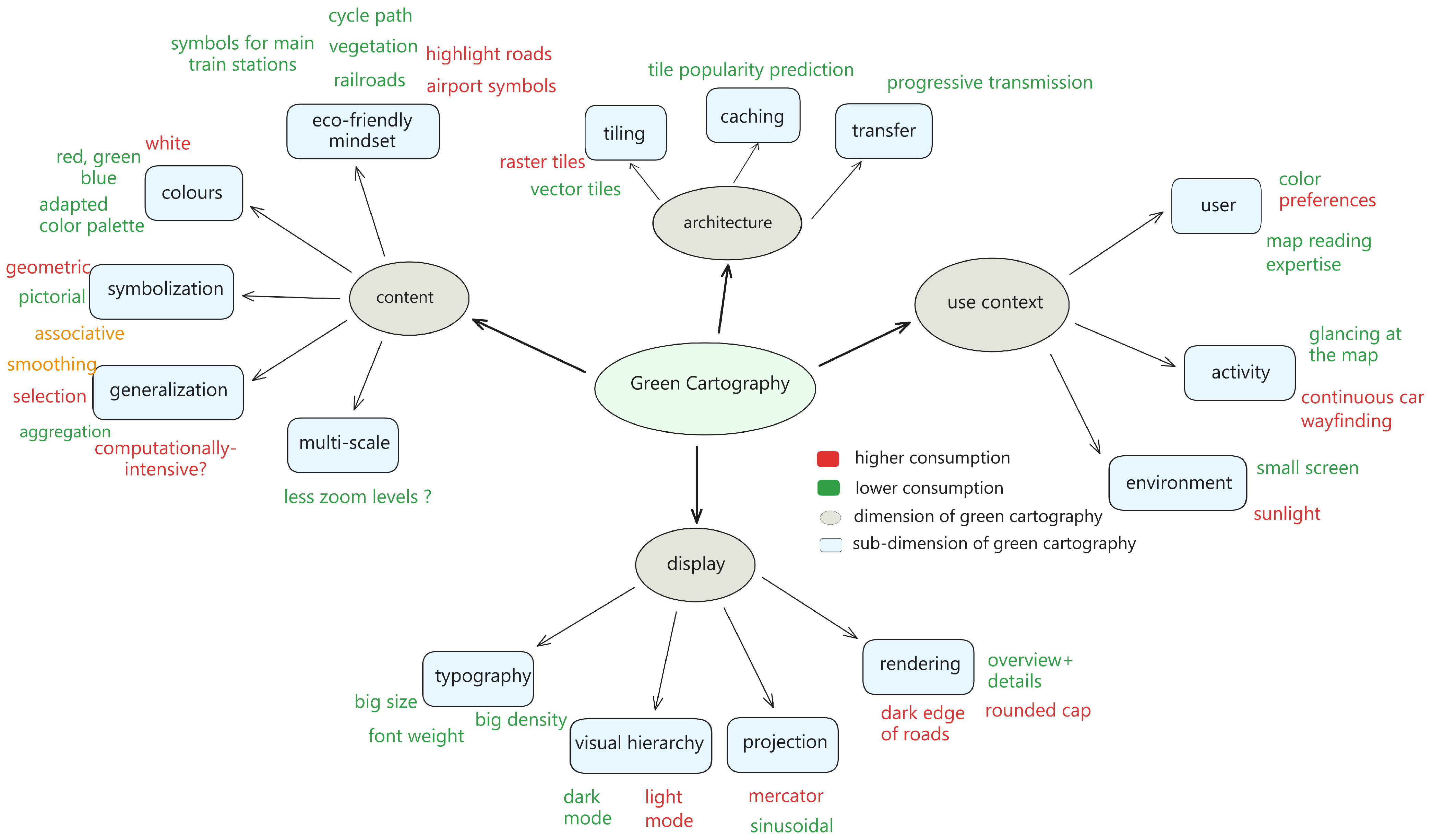
2. Green Cartography and Green Computing

There are four major sources of energy consumption for web maps: screen display, storage, map computation, and map transfer. This section reviews past research projects that propose solutions that could reduce those four different sources of energy consumption, even though most of them were not initially proposed to reduce energy consumption.
The first source is the energy consumed by the screen of the phone or the computer. The energy used by OLED displays, which are now the most common type of display [4], can be estimated with models based on the pixel values of the image to be displayed [8]. With this sort of model, different map styles can be compared to assess which one consumes more energy on the screen. Cartographic style is a design variable that can be adjusted to adapt to several user needs [9,10], and style can also be adjusted to reduce the energy consumed by the screen rendering. For instance, from a color scheme defined in a map legend, it is possible to derive a dark version of the color scheme that reduces the energy used for rendering while preserving the semantic relations between the colors in the map [11]. It is also possible to define default energy-efficient color schemes, for choropleth maps, for instance [5]. Beyond style, all cartographic design decisions (e.g., generalization, typography, projection) can be constrained by a low-energy-consumption perspective [4]. For instance, font size for toponyms has a positive influence on energy consumption when the text is rendered with dark colors and the background is rendered with light colors, which is frequent in current cartographic styles.
The second source of energy consumption is the storage of map tiles on large servers in data centers. By reducing the amount of information that is stored, we can directly reduce the energy cost. The first proposition from the literature is to replace, as much as possible, raster tiles with vector tiling techniques, as storing vector tiles seems to be less volume-intensive than storing raster tiles for the same styles and spatial extent [12]. Vector tiling techniques are slowly replacing raster tiling for maps, but the literature suggests that it would be a faster way to reduce the energy cost. When using vector tiles, another solution to reduce the storage cost is to use map generalization to simplify the data to be used at smaller scales [12,13]. In this case, the data on the server side should be stored in a multi-scale or multi-representation database [14]. To go even further in the optimization of the storage space of this multi-scale database, some researchers propose database architectures that minimize redundancies between the information stored for the different scales [15]. Other rules can be applied to both vector and raster tiles to save storage space due to the multi-scalar nature of the maps. The scale of appearance in the map can be used as a new visual variable to convey hierarchies and avoid the redundant storage of recurring map elements [16]. For instance, when zooming into a named region (a country, city, or administrative region), it is not necessary to show the toponym of this region at larger scales, because the user knows they are inside the region; removing these redundant toponyms slightly reduces the size of the tiles at larger scales.
Several techniques are also proposed to reduce the third source of energy consumption, i.e., the energy used to compute map tiles while maintaining high-quality topographic maps. Once again, using vector tiles, it is not necessary to compute raster tiles on the server anymore, even though additional computations are required on the client side [12]. It may be beneficial if a large portion of the raster tiles that are re-computed after each update are rarely visualized by users. In this case, recent research on map generalization noticed that the generalization processes were often not used in current multi-scale web maps and rather propose to use them progressively at each zoom level [17,18]. With a constant reduction in and simplification of the data across scales, we might be able to reduce the complexity of the computation of the image/vector tiles for small scales.
The last source of energy consumption is the transfer of tiles (vector and raster) during the use of the map. Several solutions have been proposed to reduce the amount of information transferred this way, though these solutions were proposed to improve performance rather than to reduce the energy used. The first one lies in the data formats used to transfer data, in particular with vector tiles or, more generally, vector data [12]. For instance, GeoJSON is now widely used and it significantly reduces the amount of information transferred compared to older formats such as GML or KML. Cartographic generalization has been proposed to reduce the other sources of energy consumption. Still, it can also serve for the tile transfer energy cost, as good multi-scale generalization can reduce the amount of zooming in and out necessary to complete a task with the map [13,18] and, as a result, reduce the number of tiles transferred to the user’s client.
Caching techniques can also be improved to reduce the energy consumed while transferring map tiles. If we minimize the number of tiles that are preventively cached without being used, unnecessary tiles are not loaded anymore. Alternatively, if we keep the tiles that might be reused later in the cache, tiles are not loaded several times during a session. The proposed solutions in the literature focus on the preventive caching of tiles: we can optimize this prefetching of tiles if the main interactions are pan and zoom [19], or by predicting the most popular tiles in a region (urban areas, density of points of interest) [20], or we can analzse the users’ preferences to prefetch the tiles they are more likely to query [21].
Finally, in the beginning of the 2000s, when web cartography was emerging, several researchers studied the progressive transmission of geographic information [22,23,24,25,26,27]. Though progressive transmission was studied to render maps quickly, the same principles can also be used to transfer multi-scale data with a minimization of the redundancy between scales. For instance, important highways are usually displayed on the map at most scales. As a result, each time a new scale is queried from the client, the same highway vector is transferred with current architectures, which seems unnecessary because this vector was already transferred.
Figure 1 shows a mindmap that summarizes examples of good and bad practices for greener cartography, found in the papers reviewed in this section. There are four dimensions in which green cartography could reduce the impact of web maps: the architecture of the system, the content of the map, the display on the screen, and the use context. For each dimension, sub-dimensions are defined with examples that promote higher or lower energy consumption. It shows that there are already plenty of ideas to make greener maps, and they just need to be considered while designing web maps.
The following sections present three small experiments to better understand the energetic cost of the tiling system of web maps. Each experiment covers a different aspect of this tiling system; Experiment 1 counts the tiles transferred when using the map Experiment 2 measures the size of the transferred tiles (Section 4), and Experiment 3 assesses the impact of map generalization on tile weight (Section 5).

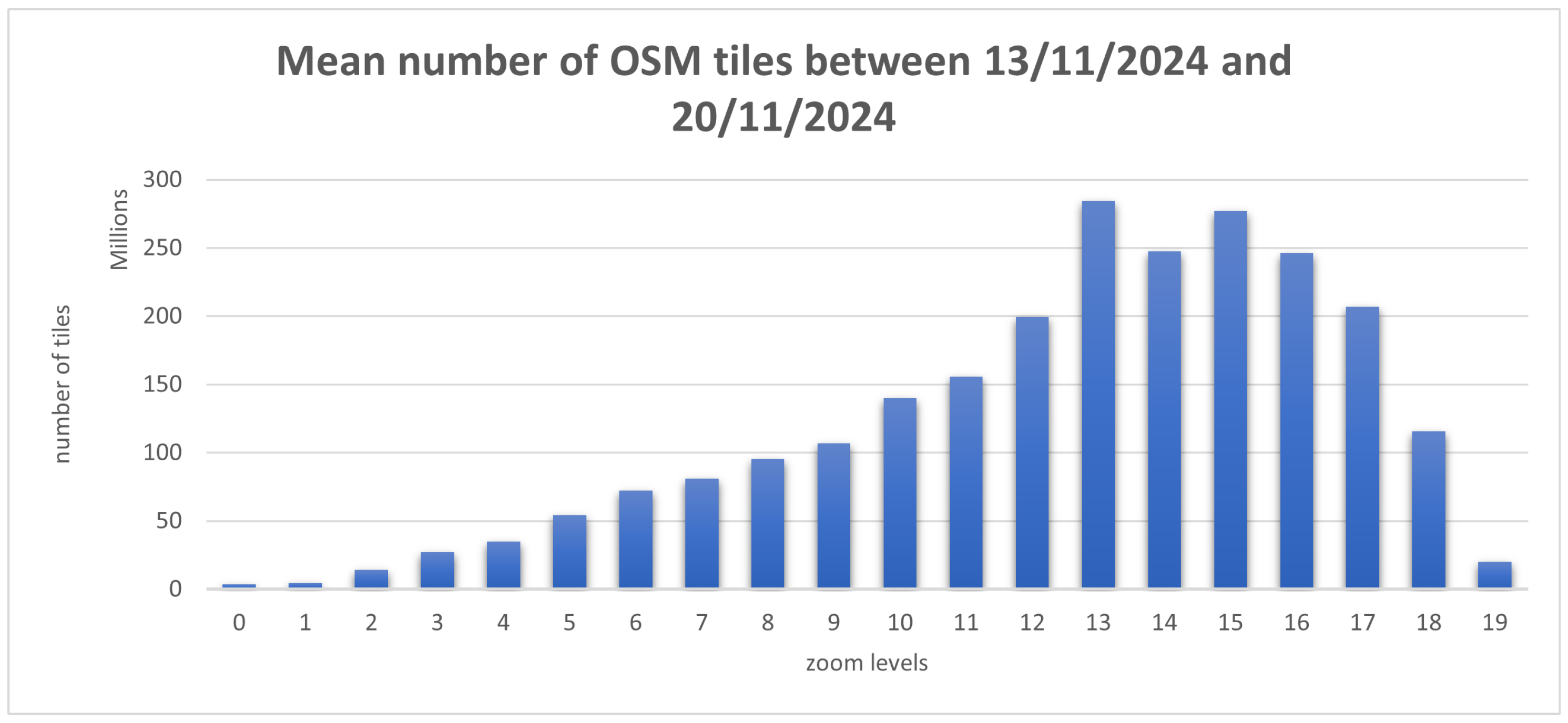
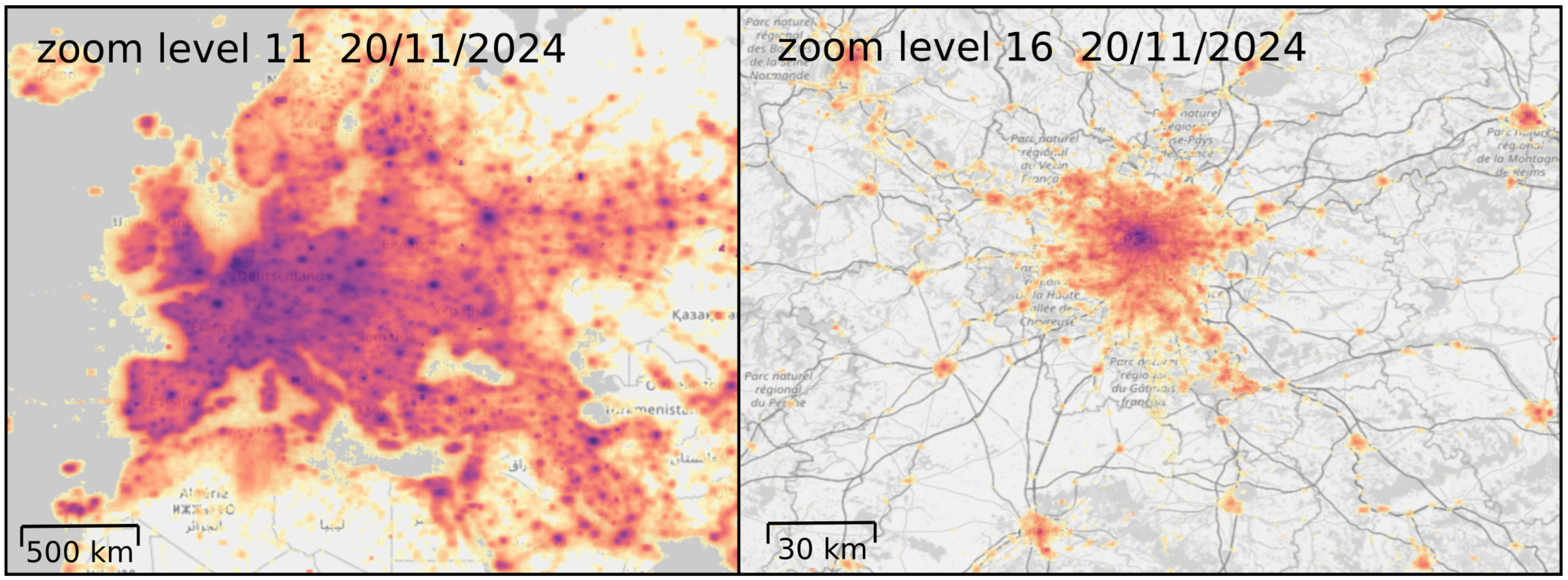
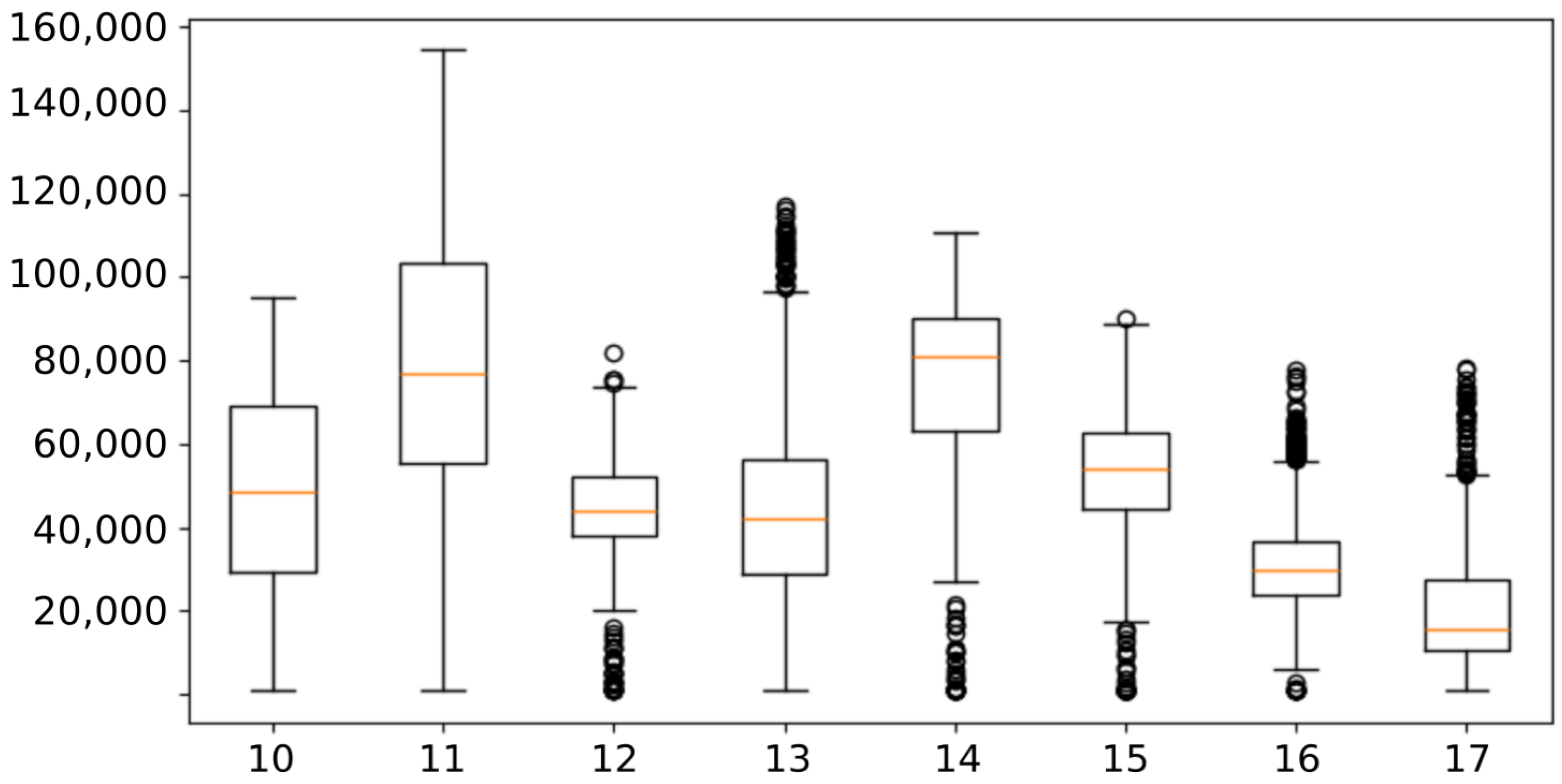
3. How Many and Which Tiles Do Map Users Use?

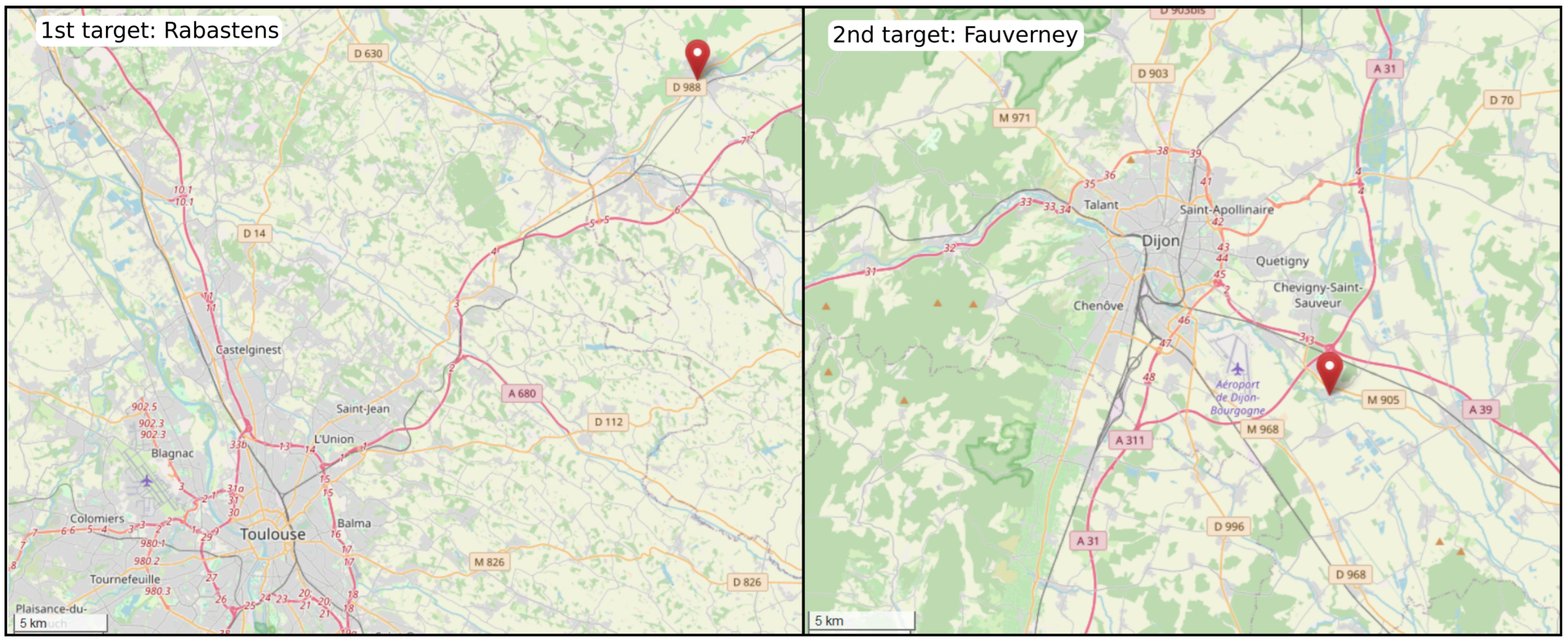
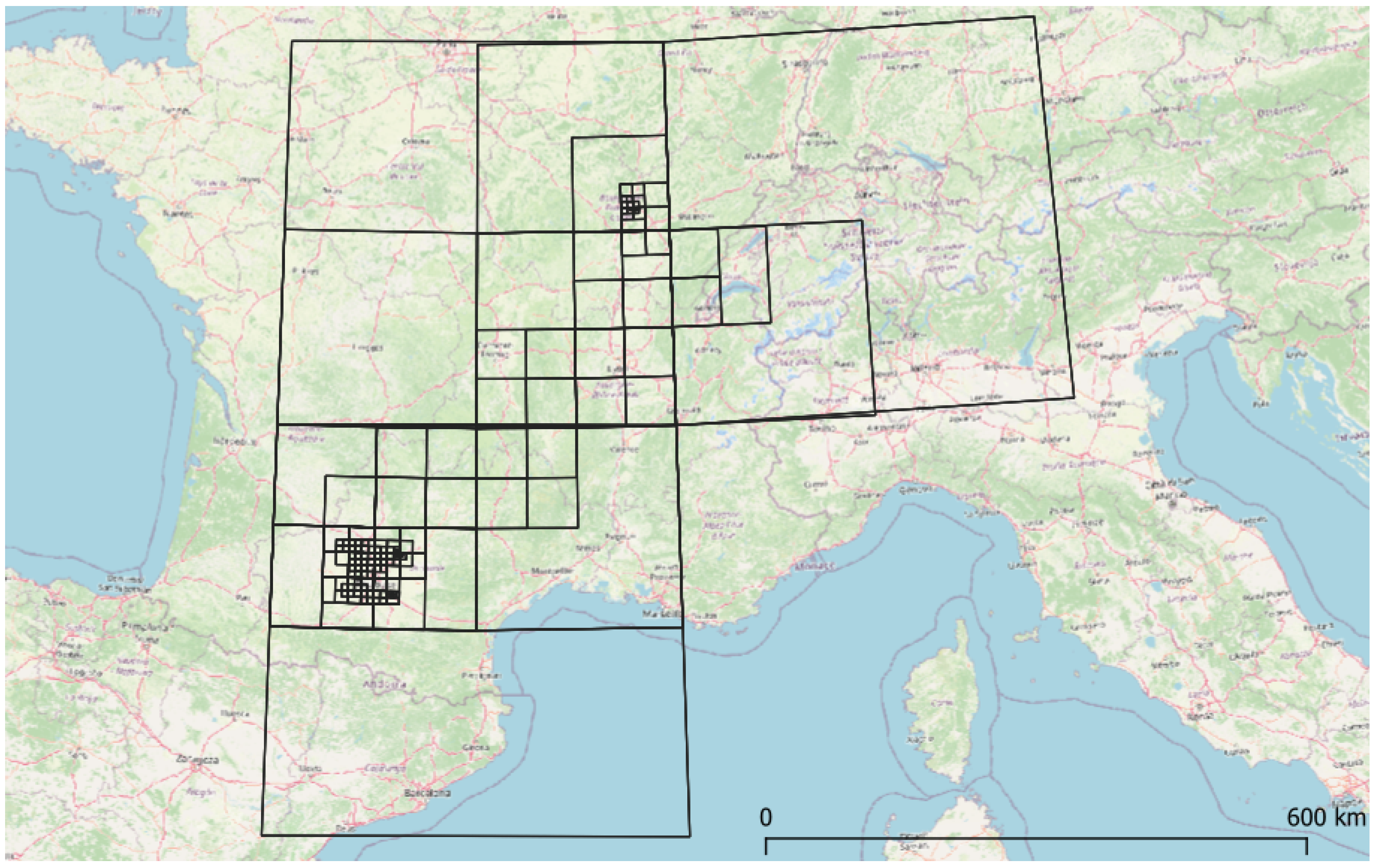
3.1. Materials and Methods
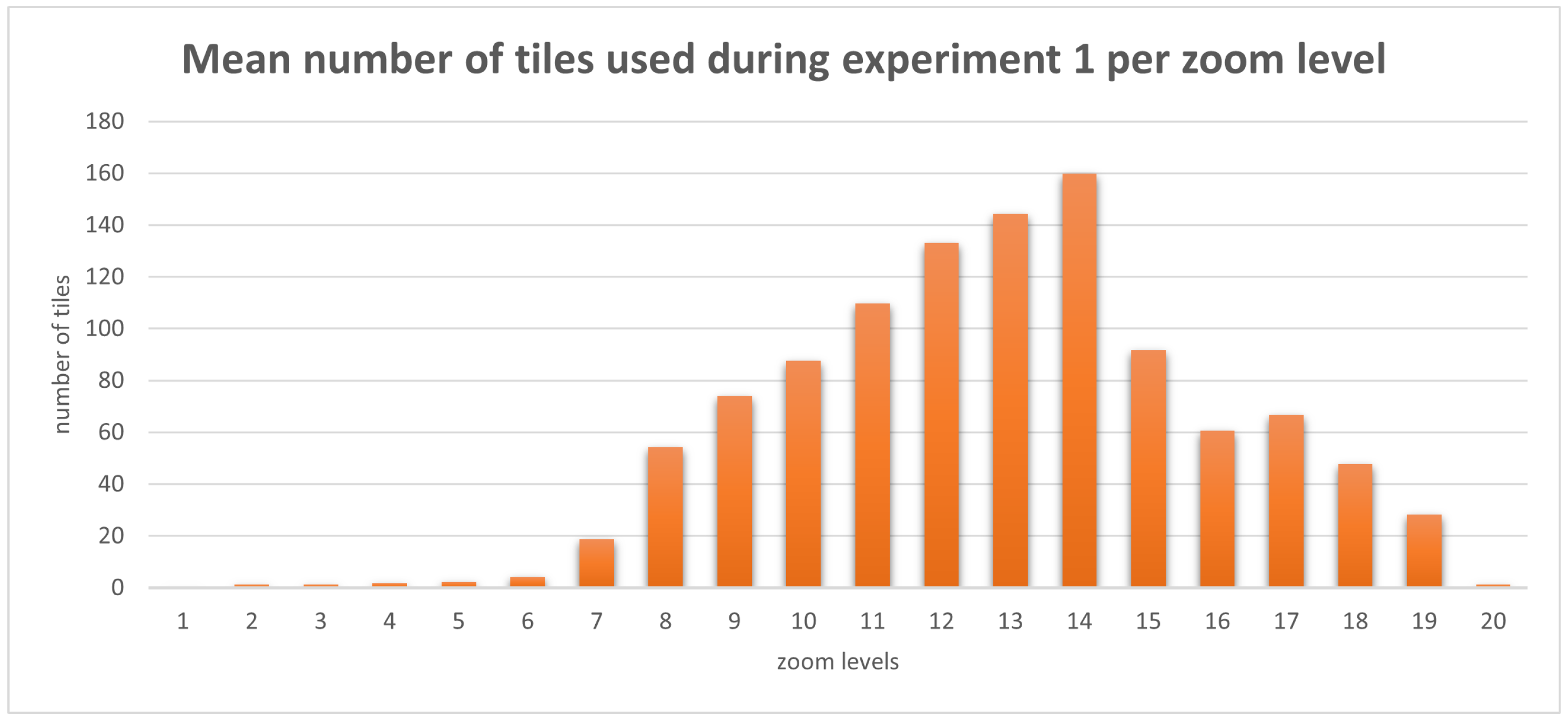
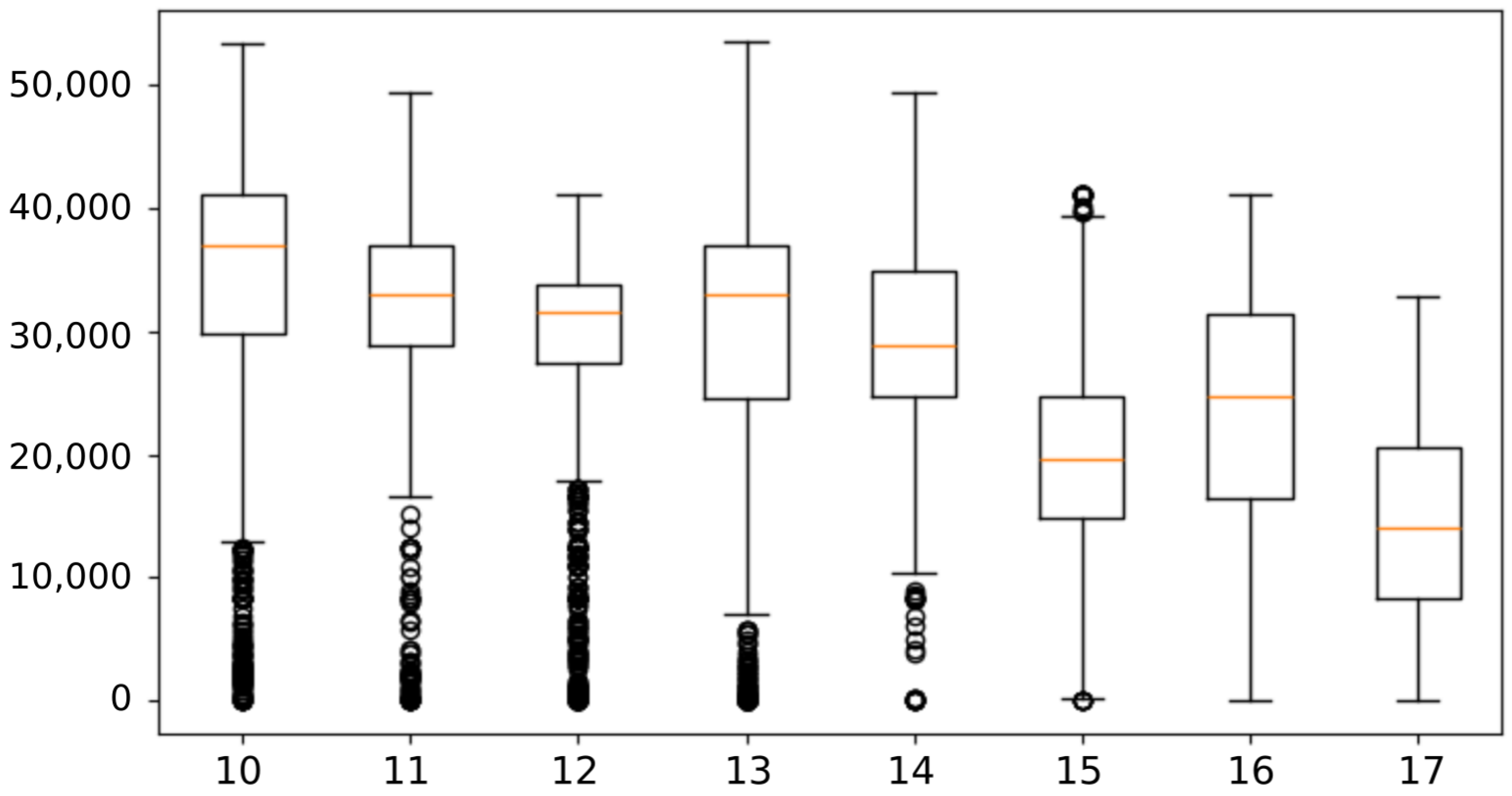
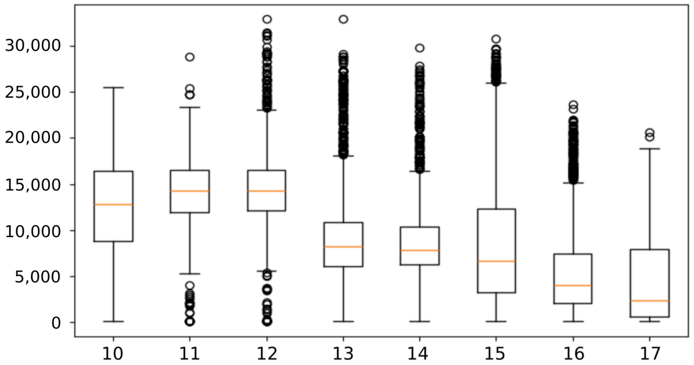
Current web mapping applications usually follow standard architectures defined by the Open Geospatial Consortium (OGC) and use tiles to render maps on the client side. These tiles can be raster or vector depending on the architecture, but in both cases, the amount of energy used to transfer those tiles is directly related to (1) the size in bits of the transferred tiles and (2) the number of tiles that are transferred during a standard use session of the map. The issue of the weight of the tiles is addressed in Section 4, and this section addresses the second cause of energy consumption, the number of tiles that are transferred during a standard use of a web map.
The goal of this first experiment, called Experiment 1 in the remainder of the paper, is to collect the tiles transferred during a standard use of a web map in order to check their number in relation to the duration of the session and their distribution over zoom levels, and to verify if these values vary with the types of interactions used. As the experiment was intended as a preliminary qualitative study, to better understand this issue of the number of tiles transferred while using the map, we selected only 9 participants who were expert users from our university, i.e., they were all trained in web cartography and were involved to some degree in research about cartography (master’s students, PhD students, and post-docs). They ran the experiment in parallel and connected to a video chat application to communicate with each other.
The selected task was to find a target in the map based on textual indications. The task was repeated twice: both targets were shown at the same time at the beginning, and the participants were supposed to start looking at the second target as soon as the first one was found. As the aim was not to spend too much time on each task, additional indications were given to the participants who did not find one target after one minute of search. The task started at zoom level 6, centred on France, and the participants had to find the churches of two small towns: Rabastens and Fauverney. The indication for Rabastens was that it was located within a radius of 30 km around Toulouse, a large French city, but not in the direct conurbation of the city. The indication was similar for Fauverney, except that it was in a 30 km radius around Dijon, another French city (Figure 2). Those two regions were chosen because none of the participants had lived there in the past; they knew where the cities were, so they were able to find them easily while navigating in the map, but they did not know any town in the surroundings of these cities. The two parts of the task (Rabastens and Fauverney) were considered to be a single block, and not considered to be a repeated task because the starting point in the map was not the same before both parts (the second part starts in Rabastens and not at zoom level 6).
As each participant was using a different computer/screen, we asked each participant to use the same internet browser, Firefox, and set the browser resolution to 1280 × 600 pixels. Each participant was asked to clear the browser cache to avoid using previously cached tiles. Comparing the number of tiles used in different mapping applications was not the goal of this experiment, so 8 of the 9 participants used the same application, a custom webpage, developed with OpenLayers, showing cartographic tiles from IGN, the French National Mapping Agency. The last participant used the default OpenStreetMap map browser (https://www.openstreetmap.org, accessed on 18 December 2024), to check if there was a noticeable difference. To determine the number of tiles transferred during the task, we asked the participants to open the network console of the web browser; each query from the client to retrieve the tiles was then printed in the console. At the end of the two tasks, the participants were asked to export the console logs as a .har file. This file was then parsed with a custom Python script to extract only the logs related to cartographic tiles. For each tile, we collected the following information: (1) the date, (2) the URL of the tile, (3) the name of the WMTS layer queried, (4) the size of the tile (in bytes), (5) the x coordinate of the tile in the tiling system, (6) the y coordinate of the tile in the tiling system, (7) the zoom level of the tile, and (8) the geographic coordinates of the tile as a WKT polygon. The output was then visualized in QGIS.
One of our hypotheses at the beginning of this experiment was that among the many possible browsing behaviors, some were more efficient in their consumption of tiles than others. To test this hypothesis, we defined different browsing behaviors (Table 1) and each participant adopted one of them while completing the task. To check the variability among the users adopting one of these behaviors, four participants adopted the same one. The first browsing behavior (BB1) was what we considered to be the standard use of a web map with a computer and a mouse: using the mouse wheel to zoom in and out slowly. We expected that this behavior would use many tiles as some unnecessary scales might be loaded on the way to the scales that were the most adapted to solve the task. The second behavior (BB2) aimed to mimic browsing with a touch screen on smartphones, but with a computer: the user only used the computer trackpad to browse the map. We also expected that this behavior would load many tiles due to clumsy and imprecise zooming gestures with the trackpad. The third browsing behavior (BB3) was to avoid panning as much as possible, and instead use zooming in and out to move across the map. We expected this behavior to generate more tiles due to unnecessary interactions, even though the unnecessary interactions may be mitigated by the tile cache if the user zooms out several times to the same tiles. The fourth behavior (BB4) was the opposite of the previous one, with a minimal use of zoom and an extensive use of panning. We expected this behavior to use many tiles due to the slower journey to the target. The next behavior (BB5) was called “center then zoom”, which means that the user had to drag the location of interest to the center of the screen before zooming, to improve the precision of zooming and avoid unnecessary interactions. We expected this behavior to require fewer tiles than the previous behavior. This is the browsing behavior that was adopted by four participants. Finally, the last browsing behavior (BB6) required the use of a window zoom instead of the mouse wheel. A window zoom is possible with Open Layers-based mapping applications; the user presses the Ctrl key while defining a rectangle on the screen. We expected this behavior to require fewer tiles due to more precision in the zooming interaction, and the possibility of skipping some zoom levels.

3.2. Results

The raw CSV files obtained during this experiment are available in a Zenodo repository (https://doi.org/10.5281/zenodo.14281428, accessed on 18 December 2024). Table 2 shows the completion time, the number of loaded tiles, and the number of tiles loaded per second for each of the participants in the experiment. As the task was easier for some participants than others due to luck (they directly zoomed close to the location of the targets), the completion time varied from 53 s to 333 s. As the number of tiles is dependent on the duration of the task and how much time the participants spent searching for the target in the map, we consider the number of tiles per second in the rest of the analysis, instead of the total number of loaded tiles. The number of tiles per second varied from 2.78 (third participant with BB5) to 12.2 (BB6).
The variability of ‘tiles per second’ values among the four participants adopting BB5 is as important as the variability among all participants (from 2.78 for participant BB5-3 to 11.03 for participant BB5-4). These results invalidate our hypothesis that there were browsing behaviors that were more energy-efficient than others, as the ‘tiles per second’ value seems more related to personal behaviors. To better understand the results, we interviewed the participants with extreme (low and high) values after the experiment. The participants with the lowest values all mentioned that they spent significant time reading the map, without any interaction. In other words, they spent a significant time in a static phase of map browsing as opposed to the transition phase [28] where the map changes due to zoom or pan. On the contrary, the participants with very high values reported that they were continuously in a transition phase, either panning or zooming, to find the target. It seems that what reduces the number of tiles used is to take the time to read maps with long static phases, instead of long transition phases. This result must be confirmed with a controlled user survey with enough participants for statistical significance.
Figure 3 shows the tiles loaded by the participant that adopted BB2 (use of the trackpad). This visualization confirms that the tiles collected during our experiment really correspond to the tiles visualized by this participant while completing the task, as the large-scale tiles are located around the cities of Toulouse and Dijon, the landmarks to find the targets. Analyzing this image, we can see that the participant searched longer for the first targets as most tiles at zoom level 14 around Toulouse were loaded, while the target around Dijon was directly found, resulting in fewer tiles loaded around the city.
A question derived from the number of tiles transferred during the use of web maps is which types of tiles are mostly used and transferred, and more precisely, which zoom levels are more used than others. Knowing the zoom levels that are more frequently transferred on the client side could help designers focus on these zoom levels to reduce energy consumption. Figure 4 shows the mean number of tiles used by the participants of the experiment, from zoom level 1 to 20 (the tile from zoom level 0 was never loaded during the experiment). As the numbers visualized in this figure are related to only one session, each unique tile can be loaded only once, as it is stored in the cache afterwards. As a result, the numbers for the smallest zoom levels are limited by the small number of tiles at these scales.
However, it can be noted that the peak in the number of tiles corresponds to zoom level 14. This result is surprising because the views at this zoom level cover a small part of the space the participant had to explore to complete the task (Figure 5). Furthermore, the tiles from zoom levels 12 and 13, where the names of the targets are visible, were also loaded a significant number of times.

3.3. Comparison with Past Studies

As Experiment 1 only represents one of the many possible map uses, the number and the zoom level of the tiles used might be different when people are using the map for navigation or when they use the search bar to directly fly to an address or a point of interest. Thus, we searched the literature for other studies analyzing the tiles consumed by map users, to compare them with our results.
OpenStreetMap distributes the logs recording the use of their default tiles (https://planet.openstreetmap.org/tile_logs/, accessed on 18 December 2024), and we can compare the distribution of those tiles across zoom levels to the data we collected in our experiment, even if the information is slightly different: the logs from OpenStreetMap aggregate the access from many users to the same tiles, while our data only record one session at a time. Figure 6 shows the distribution of the tiles used during one week (between 13 November 2024 and 20 November 2024) and shows a prominent use of the medium–large zoom levels, between 13 and 17, with peak values at zoom levels 13 and 15. The curve is not very different from the one obtained with our experimental data, though it is skewed towards the largest zoom levels, with tiles at zoom levels 16 and 17 being highly accessed. Our interpretation of these figures is that the most loaded zoom levels are not the ones where we read the map during a static phase, but the ones that are used to navigate towards a target location and scale.
The results from an experiment with many users [29] exhibit a similar pattern after logging a large number of Google Maps sessions, but they are skewed even more towards larger scales. Zoom levels 15 and 17 are the most used zoom levels, which can be explained by the most prominent interaction used in Google Maps: the search bar. When typing an address or the name of a point of interest in the search bar, Google Maps flies to the location at zoom level 17.
In addition to the distribution of tiles across zoom levels, we can also analyze the spatial distribution of those tiles. Figure 7 shows a visualization of the tiles transferred by OSM users during a day (20 November 2024), using the OSM tile access logs viewer (https://osm-tile-access-log-viewer.raifer.tech/, accessed on 18 December 2024). At zoom level 11, we can see that the use is mainly centered in Western Europe, with peak values around large cities. At zoom level 16, only the urban tiles are transferred, and the large-scale rural tiles are never visualized. It appears that OpenStreetMap is mainly used to explore cities, where the data are usually more exhaustive.

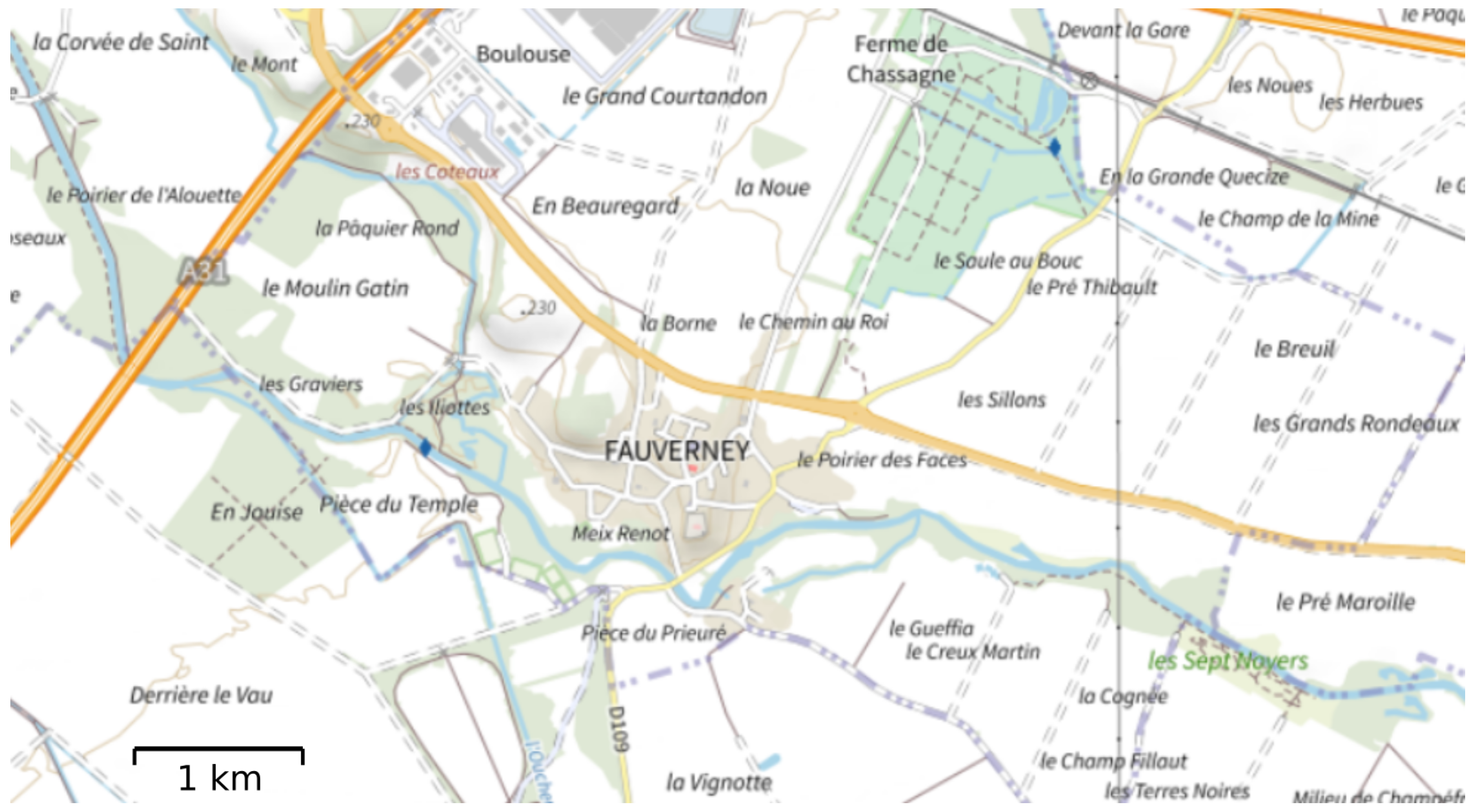
4. Comparing the Weight of Map Tiles

Studying the number of tiles transferred during the use of web maps is not enough to quantify the energy consumption during this transfer because each tile has a different size in bits, even though the size in pixels is the same ( 256 × 256 ). Figure 8 shows three tiles from OpenStreetMap at the same zoom level (10). Tile (a) weighs 47 Kb, probably due to the numerous small forest patches. Tile (b), with a similar landscape but larger forest patches, weighs 38 Kb. Tile (c), with a large portion of sea, only weighs 5 Kb. To explore these size differences quantitatively, we designed another experiment, called Experiment 2 in the paper, to collect tiles at different zoom levels.

4.1. Materials and Methods

We can see in the example in Figure 8 that size depends on the depicted landscape, and we designed a protocol to systematically collect tiles from different regions with large cities, small towns, rural areas, mountains, and coastal areas. We used the same environment as that in the previous experiment, with a Firefox browser opened and the network console printing the tile queries. This time, the zoom level was fixed and only panning was used. The task was to quickly pan for 1.5 min. After several beta tests, we decided that 1.5 min of quick pans were sufficient to collect a significant number of different tiles. The participants were given two additional instructions: (1) they were asked to avoid coming back to previously loaded tiles as much as possible, and (2) they were asked to scan as many different landscapes as possible. A tutorial was provided to obtain behaviors that were as consistent as possible among participants. At the end of the 1.5 min, the network console of the browser was saved as a .har file that was then parsed with the same Python script to obtain a CSV file of all the tiles loaded during the session. Figure 9 shows an example of the tiles collected at zoom level 16 following this protocol. The nine participants from Experiment 1 also formed the pool of participants in Experiment 2.
Following the discussion of the number of tiles used per zoom level in the previous section, we decided to collect tiles for all zoom levels between 10 and 17 (included). This protocol was reproduced for three different map styles: Plan IGN (https://www.geoportail.gouv.fr/carte, accessed on 18 December 2024) from IGN, the French National Mapping Agency; OpenCycleMap (https://www.opencyclemap.org/, accessed on 18 December 2024), which we considered to be a more complex topographic map with additional layers depicting cycling lanes and routes; and Positron Carto, which can be accessed with umap (https://umap.openstreetmap.fr, accessed on 18 December 2024), and is an example of a map with a faded topographic background, designed to include additional thematic layers on top. Without those additional layers, Positron Carto was expected to use lighter image tiles.

4.2. Results

Figure 10 shows the distribution of the tile sizes in bytes for the eight tested zoom levels (from 10 to 17) from the Plan IGN map produced by the French national mapping agency. Zoom levels 11 and 14 contain the largest tiles, while zoom levels 16 and 17 contain the smallest tiles. When observing the map at the largest two zoom levels (11 and 14), the distribution of tile sizes is not surprising, as zoom level 11 corresponds to the appearance of the toponyms of all municipalities, while zoom level 14 corresponds to the appearance of the toponyms for hamlets and similar local places (Figure 11).
Figure 12 shows the distribution of the tile sizes in bytes for the eight tested zoom levels (from 10 to 17), from the default OpenCycleMap style. It is first important to note that, contrary to our hypothesis, the tiles from OpenCycleMap are lighter than the ones from Plan IGN. As such, we can see that the tiles become lighter as the zoom level increases, zoom level 10 being the one with the largest tiles. This can be explained by the fact that as scale increases, there is no additional object depicted on the map, and almost all objects related to cycling routes are already visible at zoom level 10.
Finally, Figure 13 shows the distribution of the tile sizes in bytes for the eight tested zoom levels (from 10 to 17) from the Positron Carto style produced by CartoDB, based on OpenStreetMap data. The curve of tile sizes across zoom levels is slightly different in this case. While the largest zoom levels are still the ones containing the lightest tiles, zoom levels 11 and 12 are the ones containing the largest tiles. Zoom level 12 corresponds to the appearance of the toponyms of most municipalities, which increases the visual complexity of the map, and thus the size of the tiles. It should be noted that, as expected, the tiles are much lighter than those of the two other maps tested in the experiment, with most zoom levels containing tiles with a mean size below 10 Kb.

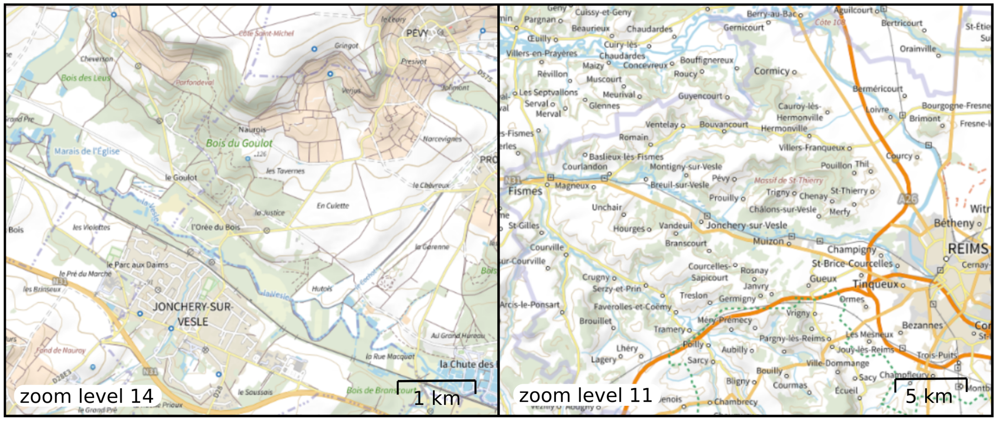
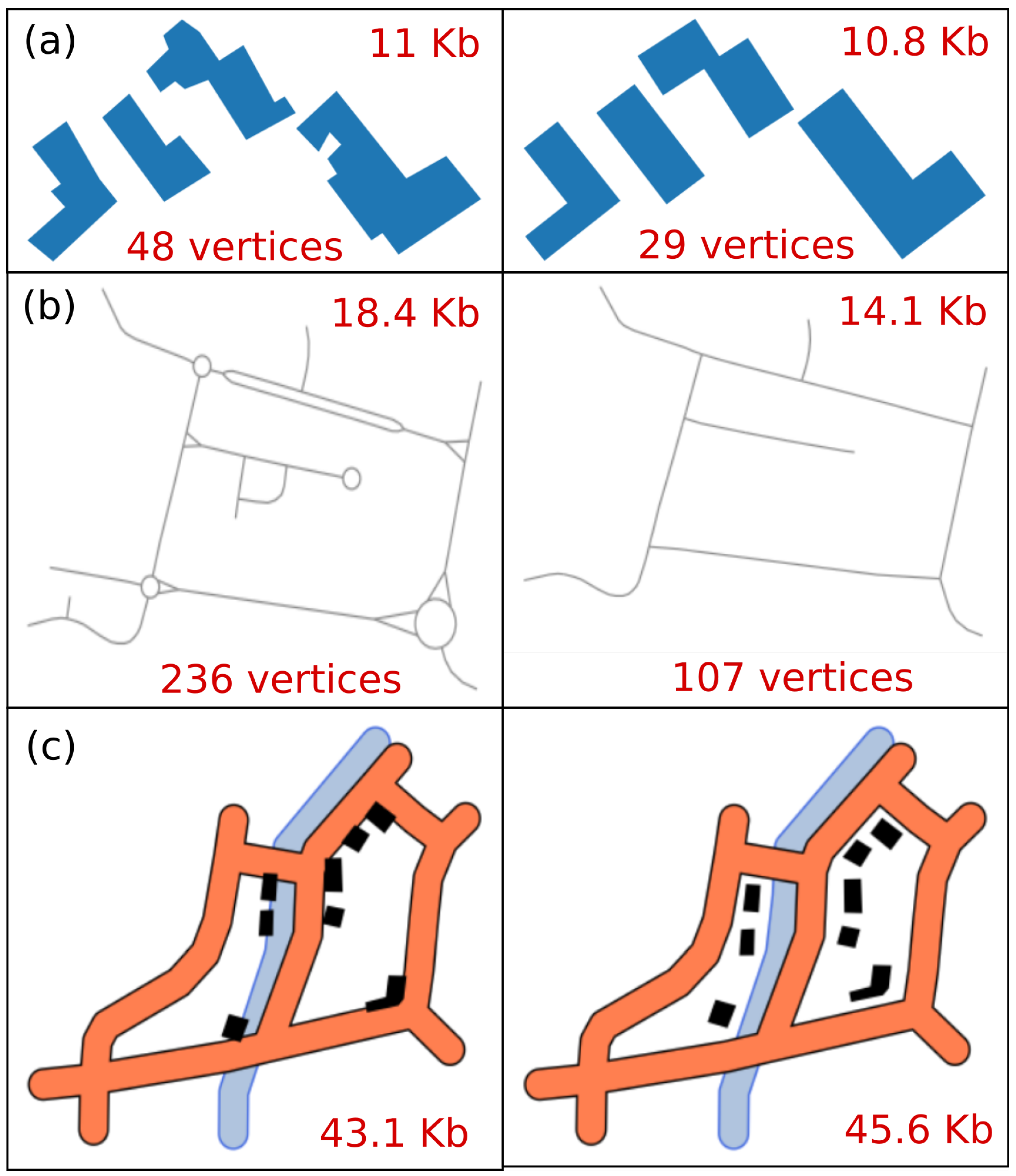
5. The Role of Map Generalization

We noted in Section 2 that authors claim that web maps should rely as much as possible on vector tiles [12,13]. There is a general belief that image tiles are larger than vector tiles for the same spatial extent, but in reality, the sizes are quite similar. Experiment 3, presented in this section, explores the size differences between vector and raster tiles. Figure 14 shows a simple topographic map tile made from four vector layers (roads, buildings, vegetation, and water areas). The image is 502 × 501 pixels and weighs 120 Kb. If we convert the four layers into GeoJSON files (the usual data format to transfer vector data), the total size is 159.19 Kb (Table 3). To make sure the vector data are lighter (to reduce storage and transfer energy), we can transform the vector data. First, we reclassified the semantic data attached to the vectors as the attribute values were sometimes very long text strings (e.g., “Forêt fermée de feuillus” for the nature of vegetation, which means “forest with deciduous trees”). We converted all the text values into integer values (e.g., “Forêt fermée de feuillus” becomes ‘0’). This reclassification process reduces the vector file size to 151.9 (5% reduction). Then, we processed the four layers with generalization algorithms that reduce the number of vertices in the geometries without any visible change in the map at this scale. We used a Douglas–Peucker algorithm [30] for roads and buildings, and the Visvalingam–Whyatt algorithm [31] for water bodies and vegetation. The total size of the vector files drops to 103.55 Kb after generalization, below the 120 Kb of the raster tile. Of course, this experiment is not sufficient to demonstrate a general benefit from the use of map generalization for web maps with vector tiles, but it shows that further studies should be carried out to find generalization operations that reduce the size of vector tiles.
In the first part of Experiment 3, presented above, generalization was used as a tool to reduce the size of a tile without changing the way the map is perceived by a human eye. In the second part of the experiment, we used generalization to visually simplify the map, to assess the impact of this transformation on the size of the tile, whether it is an image or a vector tile. On small datasets, we tested the impact of several types of map generalization operations on the size of the resulting images (Figure 15) and vector tiles. First, we processed four buildings from OpenStreetMap with the AGENT generalization model [32], which automatically chains enlargement, simplification, and squaring algorithms. In this case, generalization only results in a 2% reduction in image size (Figure 15a), while the reduction in terms of vertices is much more significant (from 48 to 29 vertices). The second example generalizes a road network using an automated selection process [33], this time resulting in a 23% reduction in image size (Figure 15b). The vector tile is much more reduced as the number of vertices is decreased by 55%. Finally, we tested the impact of a displacement algorithm [34,35] that moves the buildings that intersect the symbols of roads and rivers (Figure 15c). This time, the impact was negative on image size, and it increased by 6%, because more pixels are colored without overlaps. In this last case, the vector tile size remains unchanged as the number of vertices stays the same. Considering that map generalization usually mixes those operations (and others) to process a complete map, these measures show that the impact of map generalization on the weight of image and vector tiles is a complex problem that deserves further dedicated research.

6. Towards Energy-Efficient Maps

In our experiments, we have seen that many tiles are never visualized. Still, they are updated and recomputed frequently, a practice leading to increased energy consumption. Vector tiles would prevent some of this unnecessary computation, as styling is processed on the client side only when the tile is queried. Another solution would be to reinvestigate incremental update research [36,37,38,39,40,41,42,43]. Currently, when there is an update in the data somewhere (e.g., a new road or a new building), the complete tiles covering the new features are recomputed at all scales, sometimes including other tiles nearby, or even sometimes all the tiles across the world, because the process is global. Incremental updating proposes solutions to define the range of updates, and to propagate them across all scales/zoom levels with minimal data processing.
Experiment 1 shows that whatever the browsing behavior, map users query many tiles. But do we read all the tiles loaded during the use of a map? Or, to put it differently, do we really need all the tiles to be loaded during the use of the map? It might be interesting to study with eye tracking how much each of the loaded tiles is visualized by map users. In particular, the tiles that are preventively loaded in the cache might not all be useful. Such a study might also plead for the use of lighter tiles loaded during the transition phases because those tiles are only observed through peripheral vision [44].
We show in the results of Experiment 1 that all zoom levels are not equal in terms of use by map readers, and some levels are heavily used compared to others. If we want to make more energy-efficient maps, we need to focus on those specific zoom levels, to reduce their transfer cost, as well as the cost to render them on the screen. In our opinion, those heavily used zoom levels (zoom levels 10 to 17) are subject to improvement thanks to map generalization techniques, and we should study how much generalization can help reduce the energy cost at these zoom levels, following the short experiments presented in the previous section. We also assume that more map generalization could make each zoom level clearer and, as a result, reduce the number of zooms from the user [18]; this assumption could be tested with user surveys.
In recent years, zoom levels have become continuous values, which might be an incitement for changing the map between zoom levels to add more continuity to the zooming experience [45]. Recent Google Maps versions have slightly changed the map by adding text and points of interest at certain half-zoom levels (for example, some town names appear at zoom level 12.5). More changes between zoom levels imply more storage for these intermediate tiles. In the future, it will be necessary to find a balance between the number of zoom levels required for better usability of the map [17,45] and the energy cost of these additional levels.
Finally, even though our own experiment was not conclusive in the identification of eco-friendly map browsing behaviors, we still believe that there is an eco-friendly way to browse maps and that it should be taught to map users, or even enforced through interaction design choices. As a result, further experiments to better define eco-friendly map browsing behaviors are necessary. We could use trackers of map browsing behavior [29,46,47] on large populations of users to identify which ones generally use fewer tiles. We can also couple the tracking of interactions with more classical techniques to track the attention of the user during the exploration of the map. Eye-tracking is frequently used in cartography [48,49] and it could be used to better characterize what we identified as an efficient behavior, i.e., the use of long static phases and short transition phases. Mouse tracking [50] could also be useful to better characterize the browsing behaviors of users that tend to transfer fewer tiles than others for a similar task.

7. Conclusions

To conclude, this paper reported three short experiments to better understand the energy consumption of web maps related to tile storage and transfer. The first finding is that the number of tiles transferred during each use of a web map is significant. Second, the distribution of these tiles among zoom levels is not regular, with a peak between levels 13 and 16, though the distribution depends on the task accomplished with the map. The third finding is that the size of the tiles is irregular across zoom levels, with larger tiles often corresponding to the most heavily loaded tiles. Finally, we found that map generalization can play an important role in the mitigation of this energy consumption, but further studies are necessary to better define what its role can be in the design of greener web maps.
We are convinced that energy cost should become one of the key factors to consider when designing a map. In the future, researchers should provide evidence of good and bad practices in terms of energy consumption to help map designers move towards greener cartography.

Author Contributions

Conceptualization, Guillaume Touya and Azelle Courtial; methodology, Justin Berli, Azelle Courtial, Bérénice Le Mao, Guillaume Touya, and Laura Wenclik; software, Jérémy Kalsron; validation, Justin Berli, Azelle Courtial, Jérémy Kalsron, Bérénice Le Mao, Guillaume Touya, and Laura Wenclik; formal analysis, Guillaume Touya; data curation, Justin Berli, Azelle Courtial, Jérémy Kalsron, Bérénice Le Mao, Guillaume Touya, and Laura Wenclik; writing—original draft preparation, Guillaume Touya; writing—review and editing, Justin Berli, Azelle Courtial, Bérénice Le Mao, Jérémy Kalsron, and Laura Wenclik; visualization, Jérémy Kalsron and Guillaume Touya; supervision, Guillaume Touya; project administration, Guillaume Touya; funding acquisition, Guillaume Touya. All authors have read and agreed to the published version of the manuscript.

Funding

This project received funding from the European Research Council (ERC) under the European Union’s Horizon 2020 research and innovation programme (grant agreement No. 101003012, LostInZoom).

Institutional Review Board Statement

Not applicable.

Informed Consent Statement

Not applicable.

Data Availability Statement

The dataset supporting the results presented in this article can be found in an open Zenodo repository (https://doi.org/10.5281/zenodo.14281428, accessed on 15 December 2024).

Conflicts of Interest

The authors declare no conflicts of interest.

References

  1. Andrae, A.S.G.; Edler, T. On Global Electricity Usage of Communication Technology: Trends to 2030. Challenges 2015, 6, 117–157. [Google Scholar] [CrossRef]
  2. Williams, J.; Curtis, L. Green: The New Computing Coat of Arms? IT Prof. 2008, 10, 12–16. [Google Scholar] [CrossRef]
  3. Russell, E. 9 Things to Know About Google’s Maps Data: Beyond the Map. 2019. Available online: https://mapsplatform.google.com/resources/blog/9-things-know-about-googles-maps-data-beyond-map/ (accessed on 18 December 2024).
  4. Wu, M.; Lv, G.; Qiao, L.; Roth, R.E.; Zhu, A.X. Green Cartography: A research agenda towards sustainable development. Ann. GIS 2024, 30, 15–34. [Google Scholar] [CrossRef]
  5. Han, Y.; Wu, M.; Roth, R. Toward green cartography & visualization: A semantically-enriched method of generating energy-aware color schemes for digital maps. Cartogr. Geogr. Inf. Sci. 2021, 48, 43–62. [Google Scholar] [CrossRef]
  6. Wu, M.; Lv, G.; Yuan, L. Green Cartography and Energy-Aware Maps: Possible Research Opportunities. In New Thinking in GIScience; Li, B., Shi, X., Zhu, A.X., Wang, C., Lin, H., Eds.; Springer Nature: Singapore, 2022; pp. 197–205. [Google Scholar] [CrossRef]
  7. Belkhir, L.; Elmeligi, A. Assessing ICT global emissions footprint: Trends to 2040 & recommendations. J. Clean. Prod. 2018, 177, 448–463. [Google Scholar] [CrossRef]
  8. Dong, M.; Zhong, L. Power Modeling and Optimization for OLED Displays. IEEE Trans. Mob. Comput. 2012, 11, 1587–1599. [Google Scholar] [CrossRef]
  9. Kent, A.J.; Vujakovic, P. Cartographic Language: Towards a New Paradigm for Understanding Stylistic Diversity in Topographic Maps. Cartogr. J. 2011, 48, 21–40. [Google Scholar] [CrossRef]
  10. Christophe, S.; Hoarau, C. Expressive Map Design Based on Pop Art: Revisit of Semiology of Graphics? Cartogr. Perspect. 2013, 73, 61–74. [Google Scholar] [CrossRef]
  11. Hoarau, C. Reaching a Compromise between Contextual Constraints and Cartographic Rules: Application to Sustainable Maps. Cartogr. Geogr. Inf. Sci. 2011, 38, 79–88. [Google Scholar] [CrossRef]
  12. Gaffuri, J. Toward Web Mapping with Vector Data. In Geographic Information Science; Xiao, N., Kwan, M.P., Goodchild, M.F., Shekhar, S., Eds.; Lecture Notes in Computer Science; Springer: Berlin/Heidelberg, Germany, 2012; Volume 7478, pp. 87–101. [Google Scholar] [CrossRef]
  13. Gaffuri, J. Improving Web Mapping with Generalization. Cartogr. Int. J. Geogr. Inf. Geovisualiz. 2011, 46, 83–91. [Google Scholar] [CrossRef]
  14. Balley, S.; Parent, C.; Spaccapietra, S. Modelling geographic data with multiple representations. Int. J. Geogr. Inf. Sci. 2004, 18, 327–352. [Google Scholar] [CrossRef]
  15. van Oosterom, P. Variable-scale Topological Data Structures Suitable for Progressive Data Transfer: The GAP-face Tree and GAP-edge Forest. Cartogr. Geogr. Inf. Sci. 2005, 32, 331–346. [Google Scholar] [CrossRef]
  16. Gruget, M.; Touya, G.; Muehlenhaus, I. Missing the city for buildings? A critical review of pan-scalar map generalization and design in contemporary zoomable maps. Int. J. Cartogr. 2023, 9, 255–285. [Google Scholar] [CrossRef]
  17. Dumont, M.; Touya, G.; Duchêne, C. Designing multi-scale maps: Lessons learned from existing practices. Int. J. Cartogr. 2020, 6, 121–151. [Google Scholar] [CrossRef]
  18. Courtial, A.; Touya, G. Does Generalisation Matters in Pan-Scalar Maps? In Proceedings of the 12th International Conference on Geographic Information Science (GIScience 2023), Leibniz International Proceedings in Informatics (LIPIcs), Leeds, UK, 12–15 September 2023; Volume 277, pp. 23:1–23:6. [Google Scholar] [CrossRef]
  19. Vieira, M.R.; Bakalov, P.; Hoel, E.; Tsotras, V.J. A Spatial Caching Framework for Map Operations in Geographical Information Systems. In Proceedings of the 2012 IEEE 13th International Conference on Mobile Data Management, Bengaluru, India, 23–26 July 2012; pp. 89–98. [Google Scholar] [CrossRef]
  20. Quinn, S.; Gahegan, M. A Predictive Model for Frequently Viewed Tiles in a Web Map. Trans. GIS 2010, 14, 193–216. [Google Scholar] [CrossRef]
  21. Pan, S.; Chong, Y.; Zhang, H.; Tan, X. A Global User-Driven Model for Tile Prefetching in Web Geographical Information Systems. PLoS ONE 2017, 12, e0170195. [Google Scholar] [CrossRef]
  22. Bertolotto, M.; Egenhofer, M. Progressive Transmission of Vector Map Data over the World Wide Web. GeoInformatica 2001, 5, 345–373. [Google Scholar] [CrossRef]
  23. Buttenfield, B. Transmitting Vector Geospatial Data across the Internet. In Geographic Information Science; Egenhofer, M., Mark, D., Eds.; Lecture Notes in Computer Science; Springer: Berlin/Heidelberg, Germany, 2002; Volume 2478, pp. 51–64. [Google Scholar] [CrossRef]
  24. Sester, M.; Brenner, C. A vocabulary for a multiscale process description for fast transmission and continuous visualization of spatial data. Comput. Geosci. 2009, 35, 2177–2184. [Google Scholar] [CrossRef]
  25. Antoniou, V.; Morley, J.; Haklay, M. Tiled Vectors: A Method for Vector Transmission over the Web. In Web and Wireless Geographical Information Systems; Carswell, J.D., Fotheringham., A.S., McArdle, G., Eds.; Lecture Notes in Computer Science; Springer: Berlin/Heidelberg, Germany, 2009; Volume 5886, pp. 56–71. [Google Scholar] [CrossRef]
  26. Corcoran, P.; Mooney, P. Topologically Consistent Selective Progressive Transmission. In Advancing Geoinformation Science for a Changing World; Geertman, S., Reinhardt, W., Toppen, F., Eds.; Lecture Notes in Geoinformation and Cartography; Springer: Berlin/Heidelberg, Germany, 2011; Volume 1, pp. 519–538. [Google Scholar] [CrossRef]
  27. Glueck, M.; Khan, A.; Wigdor, D.J. Dive in! Enabling progressive loading for real-time navigation of data visualizations. In Proceedings of the SIGCHI Conference on Human Factors in Computing Systems, CHI’14, Toronto, ON, Canada, 26 April–1 May 2014; pp. 561–570. [Google Scholar] [CrossRef]
  28. Potié, Q.; Touya, G.; Wenclik, L.; Mackaness, W. Browsing Map Browsers. Abstr. ICA 2024, 7, 130. [Google Scholar] [CrossRef]
  29. Braga, V.G.; Corr, S.L.; Rodrigues, V.J.d.S.; Cardoso, K.V. Characterizing User Behavior on Web Mapping Systems Using Real-World Data. In Proceedings of the 2018 IEEE Symposium on Computers and Communications (ISCC), Natal, Brazil, 25–28 June 2018; pp. 01056–01061. [Google Scholar] [CrossRef]
  30. Douglas, D.H.; Peucker, T.K. Algorithms for the Reduction of the Number of Points Required to Represent a Digitized Line or its Caricature. Cartogr. Int. J. Geogr. Inf. Geovisualiz. 1973, 10, 112–122. [Google Scholar] [CrossRef]
  31. Visvalingam, M.; Wyatt, J.D. Line Generalization by Repeated Elimination of Points. Cartogr. J. 1993, 30, 46–51. [Google Scholar] [CrossRef]
  32. Barrault, M.; Regnauld, N.; Duchêne, C.; Haire, K.; Baeijs, C.; Demazeau, Y.; Hardy, P.; Mackaness, W.A.; Ruas, A.; Weibel, R. Integrating multi-agent, object-oriented, and algorithmic techniques for improved automated map generalisation. In Proceedings of the 20th International Cartographic Conference, ICA, Beijing, China, 6–10 August 2001; Volume 3, pp. 2110–2116. [Google Scholar]
  33. Touya, G. A Road Network Selection Process Based on Data Enrichment and Structure Detection. Trans. GIS 2010, 14, 595–614. [Google Scholar] [CrossRef]
  34. Harrie, L.E. The Constraint Method for Solving Spatial Conflicts in Cartographic Generalization. Cartogr. Geogr. Inf. Sci. 1999, 26, 55–69. [Google Scholar] [CrossRef]
  35. Sester, M. Generalization Based on Least Squares Adjustment. Int. Arch. Photogramm. Remote. Sens. 2000, 33, 931–938. [Google Scholar]
  36. Kilpeläinen, L.T.; Sarjakoski, T. Incremental generalization for multiple representations of geographic objects. In GIS and Generalization: Methodology and Practise; Muller, J.C., Lagrange, J.P., Weibel, R., Eds.; Taylor & Francis: London, UK, 1995; pp. 209–218. [Google Scholar]
  37. Harrie, L.E.; Hellström, A.K. A Prototype System for Propagating Updates Between Cartographic Data Sets. Cartogr. J. 1999, 36, 133–140. [Google Scholar] [CrossRef]
  38. Skogan, D. Towards a Rule-based Incremental Generalization System. In Proceedings of the 5th AGILE Conference on Geographic Information Science, Palma, Spain, 25–27 April 2002. [Google Scholar]
  39. Lecordix, F.; Lemarié, C. Managing Generalisation Updates in IGN Map Production. In Generalisation of Geographic Information; Mackaness, W.A., Ruas, A., Sarjakoski, L.T., Eds.; Elsevier: Amsterdam, The Netherlands, 2007; pp. 285–300. [Google Scholar] [CrossRef]
  40. Anders, K.H.; Sester, M.; Bobrich, J. Incremental Update in a MRDB. In Proceedings of the 23rd International Cartographic Conference, ICA, Moscow, Russia, 4–10 August 2007. [Google Scholar]
  41. Haunert, J.H.; Anders, K.H.; Sester, M. Hierarchical Structures for Rule-Based Incremental Generalisation. In Proceedings of the ISPRS Archives XXXVI Working Group II/2, Beijing, China, 3–11 July 2008. [Google Scholar]
  42. Zhou, S.; Regnauld, N.; Roensdorf, C. Towards a Data Model for Update Propagation in MR-DLM. In Proceedings of the 11th ICA Workshop on Generalisation and Multiple Representation, ICA, Montpellier, France, 20–21 June 2008. [Google Scholar]
  43. Straupis, T. Optimisation of generalisation re-calculation using partitioning. Abstr. ICA 2022, 5, 83. [Google Scholar] [CrossRef]
  44. Rosenholtz, R. Capabilities and Limitations of Peripheral Vision. Annu. Rev. Vis. Sci. 2016, 2, 437–457. [Google Scholar] [CrossRef]
  45. Dumont, M.; Touya, G.; Duchêne, C. More is less—Adding zoom levels in multi-scale maps to reduce the need for zooming interactions. J. Spat. Inf. Sci. 2023, 27. [Google Scholar] [CrossRef]
  46. Popelka, S.; Vojtechovska, M.; Ruzicka, O.; Beitlova, M.; Stachon, Z. Adapting to the Mobile Majority: A New Approach to Interactive Map Usability Assessment. In Proceedings of the Online User Experiments: Seeing What Map Users See Without Seeing Them, Vienna, Austria, 9 September 2024. [Google Scholar]
  47. Touya, G.; Brusq, R.; Campo, L.; Pech, V.; Wenclik, L. Recording the Use of Interactive Web Maps with ZoomTracker. Abstr. ICA 2024, 7, 176. [Google Scholar] [CrossRef]
  48. Krassanakis, V.; Cybulski, P. Eye Tracking Research in Cartography: Looking into the Future. ISPRS Int. J. Geo-Inf. 2021, 10, 411. [Google Scholar] [CrossRef]
  49. Fairbairn, D.; Hepburn, J. Eye-tracking in map use, map user and map usability research: What are we looking for? Int. J. Cartogr. 2023, 9, 231–254. [Google Scholar] [CrossRef]
  50. Krassanakis, V.; Misthos, L.M. Mouse Tracking as a Method for Examining the Perception and Cognition of Digital Maps. Digital 2023, 3, 127–136. [Google Scholar] [CrossRef]
Figure 1. Mindmap that summarizes the different dimensions of green cartography and examples cited in the literature that increase or reduce the energy consumed by web maps.
Ijgi 14 00107 g001
Figure 2. The two target towns of the first experiment and their location compared to the city cited in the textual indications.
Ijgi 14 00107 g002
Figure 3. Visualization of the tiles loaded during the experiment by the participant with behavior BB2 (used the trackpad and not the mouse). ©OpenStreetMap contributors.
Ijgi 14 00107 g003
Figure 4. Mean number of tiles loaded per participant in Experiment 1 for each zoom level.
Ijgi 14 00107 g004
Figure 5. The small town of Fauverney, the second target of the experiment, visualized at zoom level 14 in the Plan IGN map (©IGN).
Ijgi 14 00107 g005
Figure 6. Mean number of OSM tiles loaded per day for each zoom level, for the week between 13 November 2024 and 20 November 2024.
Ijgi 14 00107 g006
Figure 7. Visualization of the tiles loaded by OpenStreetMap users on 20 November 2024, from the OSM tile access logs viewer. Zoom level 11 tiles (on the left), zoom level 16 tiles (on the right).
Ijgi 14 00107 g007
Figure 8. Three tiles from OpenStreetMap at zoom level 10. Tile (a) weighs 47 Kb, tile (b) Kb, and tile (c) 5 Kb. ©OpenStreetMap contributors.
Ijgi 14 00107 g008
Figure 9. The tiles collected at zoom level 16 during the second experiment. The darker the red is, the larger the tile is (in Kb). The tiles are displayed over an OpenStreetMap background (©OpenStreetMap contributors).
Ijgi 14 00107 g009
Figure 10. Box plot of the image tiles size in bytes across zoom levels 10 to 17 with the Plan IGN map style from IGN.
Ijgi 14 00107 g010
Figure 11. Two extracts of the Plan IGN map at zoom levels 11 and 14, the ones with the largest mean size values (Source: IGN).
Ijgi 14 00107 g011
Figure 12. Box plot of the image tiles size in bytes across zoom levels 10 to 17 with the OpenCycleMap style.
Ijgi 14 00107 g012
Figure 13. Box plot of the image tiles size in bytes across zoom levels 10 to 17 with the Positron map style from CartoDB.
Ijgi 14 00107 g013
Figure 14. A raster map tile to illustrate the potential impact of map generalization on the size in Kb of the tiles.
Ijgi 14 00107 g014
Figure 15. Three different types of generalization operations and their impact on the size of image tiles. (a) Building generalization (simplification, enlargement, and squaring) slightly reduces image size. (b) Road selection significantly reduces image size. (c) Displacement increases image size as the road and river symbol parts previously hidden under buildings are now visible.
Ijgi 14 00107 g015
Table 1. The six map browsing behaviors adopted by the experiment participants.
IDBrowsing BehaviorNumber of ParticipantsExpected Impact on Tiles
BB1small zoom with mouse wheel1many tiles loaded at intermediary scales
BB2trackpad1more tiles loaded due to clumsy interactions
BB3no panning1more tiles due to unnecessary interactions
BB4mostly panning1more tiles loaded due to a slow journey to the target
BB5center then zoom4fewer tiles due to a more precise zoom
BB6window zoom1fewer tiles due to a more precise zoom
Table 2. Number of tiles loaded during the experiment for each participant.
Browsing BehaviorCompletion TimeLoaded TilesTiles per Second
BB11749755.6
BB215313839.0
BB319515057.72
BB41957623.91
BB5-11719425.5
BB5-233319085.73
BB5-32226202.78
BB5-49099311.03
BB65364812.2
Table 3. Size in Kb of the GeoJSON files constituting the map from Figure 14.
LayerInitial SizeAfter Attribute SimplificationAfter Generalization
roads71.967.351.6
buildings58.756.342.0
water5.295.203.04
vegetation23.323.16.91
complete map159.19151.9103.55
Disclaimer/Publisher’s Note: The statements, opinions and data contained in all publications are solely those of the individual author(s) and contributor(s) and not of MDPI and/or the editor(s). MDPI and/or the editor(s) disclaim responsibility for any injury to people or property resulting from any ideas, methods, instructions or products referred to in the content.

